Computational homogenization of non-stationary transport processes in masonry structures

Abstract

A fully coupled transient heat and moisture transport in a masonry structure is examined in this paper. Supported by several successful applications in civil engineering the nonlinear diffusion model proposed by Künzel [1] is adopted in the present study. A strong material heterogeneity together with a significant dependence of the model parameters on initial conditions as well as the gradients of heat and moisture fields vindicates the use of a hierarchical modeling strategy to solve the problem of this kind. Attention is limited to the classical first order homogenization in a spatial domain developed here in the framework of a two step (meso-macro) multi-scale computational scheme (FE² problem). Several illustrative examples are presented to investigate the influence of transient flow at the level of constituents (meso-scale) on the macroscopic response including the effect of macro-scale boundary conditions. A two-dimensional section of Charles Bridge subjected to actual climatic conditions is analyzed next to confirm the suitability of algorithmic format of FE² scheme for the parallel computing.

1 Introduction

Historical masonry structures all over the world enjoy constant attention by many entities including technical audience and public authorities. When subject to restoration these structures naturally invite complex analyses combining both experimental work [2] and numerical simulations [3]. Even after closing the scheduled reconstruction steps a continuation of in-situ monitoring is now becoming almost standard allowing the engineers not only to evaluate the current state of the structure but also to improve the predictive capability of theoretical models being supported by up to date material data and instantaneous measurements of the state of stress and deformation. A particularly vivid example of this line of inquiry is the Charles Bridge information system [4] integrating detailed geometrical description of the bridge including changes resulting from previous reconstructions, historical and contemporary materials forming the bridge as well as novel materials and technologies used to improve its durability and serviceable life. The available results of long-term measurements of temperature and moisture fields, time-dependent displacement data, complemented by advanced methods of computational analysis then open the way to incorporate multi-physics, multi-scale, time-dependent and three-dimensional aspects of the problem to create a realistic computational model of such a complex structure.

These issues have been supported by our recent study [5] devoted to the homogenization of masonry walls with emphases on the effect of imperfect hydraulic contact. On the one hand, it has been demonstrated that the introduction of interface transition zone at the mesostructural level, considerably complicating the computational matter, is essentially negligible for the prediction of effective properties. On the other hand, an accompanied parametric study has shown a substantial dependence of the homogenized properties on both the initial and loading conditions. Keeping the format of a simplified uncoupled multi-scale scheme with several successful applications particularly in civil engineering [3, 6, 7, to cite a few] would require performing the homogenization analysis for various values of water content and certain referenced initial values of temperature and relative humidity to construct the homogenized macro-scale retention curves. Utilizing these curves in an independent macroscopic study would considerably increase the computational efficiency since avoiding a time consuming down scaling for the parameters update at every macroscopic time step. Unfortunately, an observed strong dependence of the effective properties on the applied macroscopic gradients may lead to an enormous database of these response functions essentially loosing the advantage over a full-fledged coupled multi-scale framework. This issue together with the possibility of including the mesostructural morphology and mesostructural material behavior in the macro-level, where typical structures are analyzed, without the need for assigning the fine-scale details to the entire structure thus motivated the developments in this paper towards an iterative FE² algorithm much similar to that presented in [8].

Owing to the finite size of the representative volume element on meso-scale we adopt a variationally consistent homogenization developed in [8] to reflect a certain size dependency of distributions of macroscopic fields due to higher order terms appearing on the left hand side of macroscopic balance equations when a non-linear transient flow is assumed on both the macro and meso-scale. A short numerical study of this topic is presented in Section 4.1 preceded by the theoretical formulation in Section 3. Section 4.2 then investigates the influence of macroscopic finite element mesh and application of the associated loading conditions in FE² scheme on the accuracy of evolution of macroscopic moisture and temperature fields. The obtained results are then utilized in Section 4.3 devoted to the parallel format of the underlying multi-scale analysis performed for a two-dimensional section of Charles Bridge. Summary of the essential findings is available in Section 5. To keep the paper self-contained a short overview of the adopted constitutive model is provided in Section 2.

In the following text, $a$ and $\mathsf{A}$ denote a vector and a symmetric second-order tensor, respectively. The symbol $\mbox{\boldmath$\nabla$}=\left\{\displaystyle{{\partial}/{\partial{x}}},\displaystyle{{\partial}/{\partial{y}}},\displaystyle{{\partial}/{\partial{z}}}\right\}^{\sf T}$ stands for the gradient representation. All materials are assumed locally isotropic.

2 Material model

The literature offers a manifold of material models that allow for the description of coupled heat and moisture transport. An extensive overview of transport models is presented in the monograph by Černý and Rovnaníková [9]. Among others the non-linear diffusion model proposed by Künzel holds a great potential for an accurate description of transport processes in building engineering including masonry structures and will be adopted here to follow up our previous works in this area [10, 5].

Künzel derived the coupled system of energy and mass balance equations based on concepts put forward by Krischer and Kiessl, see e.g. [11, 1]. In [12] Krischer identified two transport mechanisms for material moisture, one being the vapor diffusion and the other being described as a capillary water movement. In other words, Krischer introduced the gradient of partial pressure in the air as the driving force for the water vapor transport and the gradient of liquid moisture content as the driving force for the water transport. Kiessl further extended the diffusion model of Krischer and developed in  [13] his own original version. The unification for the description of moisture transport in the hygroscopic $\varphi\leq 0.9$ and overhygroscopic $\varphi>0.9$ range ($\varphi$ is the relative humidity) was achieved with the help of moisture potential, which brought several advantages particularly a very simple expression for the moisture transport across interfaces. On the other hand, the definition of moisture potential in the overhygroscopic range was too artificial, and Kiessl introduced it without any theoretical background, see [9].

For the description of simultaneous water and water vapor transport Künzel neglected the liquid water and water vapor convection driven by gravity and total pressure as well as enthalpy changes due to liquid flow and choose the relative humidity $\varphi$ as the only moisture potential for both hygroscopic and overhygroscopic range. He also divided overhygroscopic region into two sub-ranges - capillary water region and supersaturated region, where different conditions for water and water vapor transport are considered. In comparison with Kiessl’s or Krischer’s model Künzel’s model introduces several simplifications. Nevertheless, the proposed model describes all substantial phenomena of the heat and moisture transport in building materials and the predicted results comply well with the experimentally obtained data [5].

Employing the classical Fick’s law for the description of water vapor diffusion, Kelvin’s law to simulate the transport of liquid water and Fourier’s law to account for the flow of heat energy the Künzel model integrates into the energy balance equation

$$\frac{\mathrm{d}H}{\mathrm{d}\theta}\frac{\mathrm{d}\theta}{\mathrm{d}t}=\mbox{\boldmath$\nabla$}^{\mathrm{T}}[\lambda\mbox{\boldmath$\nabla$}\theta]+h_{v}\mbox{\boldmath$\nabla$}^{\mathrm{T}}[\delta_{p}\mbox{\boldmath$\nabla$}\{\varphi p_{\mathrm{sat}}(\theta)\}],$$ (1)

and the conservation of mass equation

$$\frac{\mathrm{d}w}{\mathrm{d}\varphi}\frac{\mathrm{d}\varphi}{\mathrm{d}t}=\mbox{\boldmath$\nabla$}^{\mathrm{T}}[D_{\varphi}\mbox{\boldmath$\nabla$}\varphi]+\mbox{\boldmath$\nabla$}^{\mathrm{T}}[\delta_{p}\mbox{\boldmath$\nabla$}\{\varphi p_{\mathrm{sat}}(\theta)\}]\,,$$ (2)

where $H$ is the enthalpy of the moist building material, $w$ is the water content of the building material, $\lambda$ is the thermal conductivity, $D_{\varphi}$ is the liquid conduction coefficient, $\delta_{p}$ is the water vapor permeability, $h_{v}$ is the evaporation enthalpy of the water, $p_{\mathrm{sat}}$ is the water vapor saturation pressure, $\theta$ is the temperature and $\varphi$ is the relative humidity. The material parameters, both measured and functionally derived, that enter the above equations are summarized for the sake of completeness in A, see also [11, 14] for more detailed discussion on this subject. Note that the second term on the right hand side of Eq. (1) represents the change of enthalpy due to phase transition being considered the only heat source or sink.

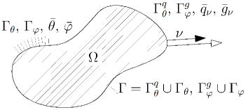
Figure 1: A two dimensional region

Application of principal of virtual work then yields the weak form of these two balance equations

$$\int_{\Omega}\delta\theta\frac{\mathrm{d}H}{\mathrm{d}\theta}\frac{\mathrm{d}\theta}{\mathrm{d}t}\mathrm{d}\Omega+\int_{\Omega}\{\mbox{\boldmath$\nabla$}\delta\theta\}^{\mathrm{\textsf{T}}}\left[\{\mathchoice{\displaystyle\mathbf{\lambda}}{\textstyle\mathbf{\lambda}}{\scriptstyle\mathbf{\lambda}}{\scriptscriptstyle\mathbf{\lambda}}\mbox{\boldmath$\nabla$}\theta\}+h_{v}\left\{\mathchoice{\displaystyle\mathbf{\delta}}{\textstyle\mathbf{\delta}}{\scriptstyle\mathbf{\delta}}{\scriptscriptstyle\mathbf{\delta}}_{p}\varphi\frac{\mathrm{d}p_{\mathrm{sat}}}{\mathrm{d}\theta}\mbox{\boldmath$\nabla$}\theta\right\}\right]\mathrm{d}\Omega+$$

$$+\int_{\Omega}\left\{\mbox{\boldmath$\nabla$}\delta\varphi\right\}^{\mathrm{\textsf{T}}}\left[h_{v}\{\mathchoice{\displaystyle\mathbf{\delta}}{\textstyle\mathbf{\delta}}{\scriptstyle\mathbf{\delta}}{\scriptscriptstyle\mathbf{\delta}}_{p}p_{\mathrm{sat}}\mbox{\boldmath$\nabla$}\varphi\}\right]\mathrm{d}\Omega-\int_{\Gamma^{\bar{q}}_{\theta}}\delta\theta\,\bar{q}_{\nu}\mathrm{d}\Gamma=0,$$ (3)

$$\int_{\Omega}\delta\varphi\frac{\mathrm{d}w}{\mathrm{d}\varphi}\frac{\mathrm{d}\varphi}{\mathrm{d}t}\mathrm{d}\Omega++\int_{\Omega}\{\mbox{\boldmath$\nabla$}\delta\varphi\}^{\mathrm{\textsf{T}}}\left[\{{D_{\varphi}}\mbox{\boldmath$\nabla$}\varphi\}+\{\mathchoice{\displaystyle\mathbf{\delta}}{\textstyle\mathbf{\delta}}{\scriptstyle\mathbf{\delta}}{\scriptscriptstyle\mathbf{\delta}}_{p}p_{\mathrm{sat}}\mbox{\boldmath$\nabla$}\varphi\}\right]\mathrm{d}\Omega+$$

$$+\int_{\Omega}\left\{\mbox{\boldmath$\nabla$}\delta\theta\right\}^{\mathrm{\textsf{T}}}\left\{\mathchoice{\displaystyle\mathbf{\delta}}{\textstyle\mathbf{\delta}}{\scriptstyle\mathbf{\delta}}{\scriptscriptstyle\mathbf{\delta}}_{p}\varphi\frac{\mathrm{d}p_{\mathrm{sat}}}{\mathrm{d}\theta}\mbox{\boldmath$\nabla$}\theta\right\}\mathrm{d}\Omega-\int_{\Gamma^{\bar{g}}_{\varphi}}\delta\varphi\,\bar{g}_{\nu}\mathrm{d}\Gamma=0,$$ (4)

to be solved numerically for the prescribed boundary and initial conditions, see Fig. 1 for the definition of prescribed boundary terms and domain representation. Owing to a strong nonlinear dependence of material parameters on both temperature and moisture fields, recall A, the Newton-Raphson method is generally needed to solve the resulting discretized system of equations.

3 First order homogenization of non-stationary coupled heat and moisture transport

The present section derives the governing equations of the coupled heat and moisture transport in the framework of coupled two-scale analysis of FE² type. In this regard it is presumed that the homogenized macro-scale fields are found from the solution of a certain sub-scale (meso-scale) problem performed on a representative volume element (RVE) being identical, at least in a statistical sense, to a real meso-structure from both the geometrical and material composition point of view. Such an RVE is then usually termed the statistically equivalent periodic unit cell (SEPUC) [15]. Examples of such SEPUCs for both regular as well as irregular masonry walls adopted herein are plotted in Fig. 6(d)(e). It has been advocated in [8] that for a finite size RVE the assumption of transient flow on both the macro and meso-scale introduces certain non-local, size dependent, terms in equations governing the macroscopic response. Some numerical simulations addressing this issue are presented in Section 4.1, whilst the theoretical grounds are provided next following closely, although in more abbreviated format, the variationally consistent homogenization outlined in detail in [8].

To introduce this subject suppose that a local field $a$ can be replaced by a spatially homogenized one $\langle{a}\rangle$ such that

$$\int_{\Omega}a\,\mathrm{d}\Omega \approx \int_{\Omega}\left\langle a\right\rangle_{\Box}\mathrm{d}\Omega=\int_{\Omega}\left(\frac{1}{\left|\Omega_{\Box}\right|}\int_{\Omega_{\Box}}a\,\mathrm{d}\Omega_{\Box}\right)\mathrm{d}\Omega,$$ (5)

$$\int_{\Gamma}a\,\mathrm{d}\Gamma \approx \int_{\Gamma}\left\langle a\right\rangle_{\Box}\mathrm{d}\Gamma=\int_{\Gamma}\left(\frac{1}{\left|\Gamma_{\Box}\right|}\int_{\Gamma_{\Box}}a\,\mathrm{d}\Gamma_{\Box}\right)\mathrm{d}\Gamma,$$ (6)

where $\Omega_{\Box}$ and $\Gamma_{\Box}$ represent the internal and boundary parts of the SEPUC. In what follows, owing to the space limitation, we shall treat only the energy balance equation (3) which upon employing Eqs. (5) and (6) becomes

$$\int_{\Omega}\left\langle\delta\theta\frac{\mathrm{d}H}{\mathrm{d}\theta}\frac{\mathrm{d}\theta}{\mathrm{d}t}\right\rangle_{\Box}\mathrm{d}\Omega+\int_{\Omega}\left\langle\{\mbox{\boldmath$\nabla$}\delta\theta\}^{\mathrm{\textsf{T}}}\left[\{\mathchoice{\displaystyle\mathbf{\lambda}}{\textstyle\mathbf{\lambda}}{\scriptstyle\mathbf{\lambda}}{\scriptscriptstyle\mathbf{\lambda}}\mbox{\boldmath$\nabla$}\theta\}+h_{v}\left\{\mathchoice{\displaystyle\mathbf{\delta}}{\textstyle\mathbf{\delta}}{\scriptstyle\mathbf{\delta}}{\scriptscriptstyle\mathbf{\delta}}_{p}\varphi\frac{\mathrm{d}p_{\mathrm{sat}}}{\mathrm{d}\theta}\mbox{\boldmath$\nabla$}\theta\right\}\right]\right\rangle_{\Box}\mathrm{d}\Omega+$$

$$+\int_{\Omega}\left\langle\{\mbox{\boldmath$\nabla$}\delta\varphi\}^{\mathrm{\textsf{T}}}\left[h_{v}\{\mathchoice{\displaystyle\mathbf{\delta}}{\textstyle\mathbf{\delta}}{\scriptstyle\mathbf{\delta}}{\scriptscriptstyle\mathbf{\delta}}_{p}p_{\mathrm{sat}}\mbox{\boldmath$\nabla$}\varphi\}\right]\right\rangle_{\Box}\mathrm{d}\Omega-\int_{\Gamma^{\bar{q}}_{\theta}}\left\langle\delta\theta\,\bar{q}_{\nu}\right\rangle_{\Box}\mathrm{d}\Gamma=0.$$ (7)

In the spirit of the first order homogenization it is assumed that the macroscopic temperature and relative humidity vary only linearly over the SEPUC. This can be achieved by loading its boundary by the prescribed temperature $\Theta^{\mathrm{hom}}$ and relative humidity $\Phi^{\mathrm{hom}}$ derived from the uniform macroscopic temperature $\mbox{\boldmath$\nabla$}\Theta$ and relative humidity $\mbox{\boldmath$\nabla$}\Phi$ gradients. In such a case the local temperature and relative humidity inside the SEPUC admit the following decomposition

$$\theta(\mbox{\boldmath$x$}) = \Theta(\mbox{\boldmath$X$}^{0})+\{\mbox{\boldmath$\nabla$}\Theta\}^{\mathrm{\textsf{T}}}\{\mbox{\boldmath$x$}-\mbox{\boldmath$X$}^{0}\}+\theta^{*}(\mbox{\boldmath$x$})=\Theta^{\mathrm{hom}}(\mbox{\boldmath$x$})+\theta^{*}(\mbox{\boldmath$x$}),$$ (8)

$$\varphi(\mbox{\boldmath$x$}) = \Phi(\mbox{\boldmath$X$}^{0})+\{\mbox{\boldmath$\nabla$}\Phi\}^{\mathrm{\textsf{T}}}\{\mbox{\boldmath$x$}-\mbox{\boldmath$X$}^{0}\}+\varphi^{*}(\mbox{\boldmath$x$})\,=\Phi^{\mathrm{hom}}(\mbox{\boldmath$x$})+\varphi^{*}(\mbox{\boldmath$x$}),$$ (9)

where $\theta^{*}(\mbox{\boldmath$x$})$ and $\varphi^{*}(\mbox{\boldmath$x$})$ are the fluctuations of local fields superimposed onto linearly varying quantities $\Theta^{\mathrm{hom}}(\mbox{\boldmath$x$})$ and $\Phi^{\mathrm{hom}}(\mbox{\boldmath$x$})$ . The temperature $\Theta(\mbox{\boldmath$X$}^{0})$ and the moisture $\Phi(\mbox{\boldmath$X$}^{0})$ at the reference point $\mbox{\boldmath$X$}^{0}$ are introduced to link the local fields to their macroscopic counterparts. For convenience the SEPUC is typically centered at $\mbox{\boldmath$X$}^{0}$. Henceforth, the local fluctuations will be demanded to be periodic, i.e. the same values are enforced on the opposite sides of a rectangular SEPUC.

Next, substituting Eqs. (8) and (9) into Eq. (7) and collecting the terms corresponding to $\delta\Theta^{\mathrm{hom}}$, $\delta\Phi^{\mathrm{hom}}$ and $\delta\theta^{*}$, $\delta\varphi^{*}$ splits the original problem (3) into the homogenized (macro-scale) problem

$$\int_{\Omega}\left\langle\{\delta\Theta^{\mathrm{hom}}\}\frac{\mathrm{d}H}{\mathrm{d}\theta}\frac{\mathrm{d}\theta}{\mathrm{d}t}\right\rangle_{\Box}\mathrm{d}\Omega+\int_{\Omega}\left\langle\{\mbox{\boldmath$\nabla$}\delta\Theta^{\mathrm{hom}}\}^{\mathrm{\textsf{T}}}\left[\{\mathchoice{\displaystyle\mathbf{\lambda}}{\textstyle\mathbf{\lambda}}{\scriptstyle\mathbf{\lambda}}{\scriptscriptstyle\mathbf{\lambda}}\mbox{\boldmath$\nabla$}\theta\}+h_{v}\left\{\mathchoice{\displaystyle\mathbf{\delta}}{\textstyle\mathbf{\delta}}{\scriptstyle\mathbf{\delta}}{\scriptscriptstyle\mathbf{\delta}}_{p}\varphi\frac{\mathrm{d}p_{\mathrm{sat}}}{\mathrm{d}\theta}\mbox{\boldmath$\nabla$}\theta\right\}\right]\right\rangle_{\Box}\mathrm{d}\Omega+$$

$$+\int_{\Omega}\left\langle\{\mbox{\boldmath$\nabla$}\delta(\Phi^{\mathrm{hom}})\}^{\mathrm{\textsf{T}}}\left[h_{v}\{\mathchoice{\displaystyle\mathbf{\delta}}{\textstyle\mathbf{\delta}}{\scriptstyle\mathbf{\delta}}{\scriptscriptstyle\mathbf{\delta}}_{p}p_{\mathrm{sat}}\mbox{\boldmath$\nabla$}\varphi\}\right]\right\rangle_{\Box}\mathrm{d}\Omega-\int_{\Gamma^{\bar{q}}_{\theta}}\left\langle\{\delta\Theta^{\mathrm{hom}}\}\,\bar{q}_{\nu}\right\rangle_{\Box}\mathrm{d}\Gamma=0,$$ (10)

and the local sub-scale (meso-scale) problem

$$\int_{\Omega}\left\langle\{\delta\theta^{*}\}\frac{\mathrm{d}H}{\mathrm{d}\theta}\frac{\mathrm{d}\theta}{\mathrm{d}t}\right\rangle_{\Box}\mathrm{d}\Omega+\int_{\Omega}\left\langle\{\mbox{\boldmath$\nabla$}\delta\theta^{*}\}^{\mathrm{\textsf{T}}}\left[\{\mathchoice{\displaystyle\mathbf{\lambda}}{\textstyle\mathbf{\lambda}}{\scriptstyle\mathbf{\lambda}}{\scriptscriptstyle\mathbf{\lambda}}\mbox{\boldmath$\nabla$}\theta\}+h_{v}\left\{\mathchoice{\displaystyle\mathbf{\delta}}{\textstyle\mathbf{\delta}}{\scriptstyle\mathbf{\delta}}{\scriptscriptstyle\mathbf{\delta}}_{p}\varphi\frac{\mathrm{d}p_{\mathrm{sat}}}{\mathrm{d}\theta}\mbox{\boldmath$\nabla$}\theta\right\}\right]\right\rangle_{\Box}\mathrm{d}\Omega+$$

$$+\int_{\Omega}\left\langle\{\mbox{\boldmath$\nabla$}\delta\varphi^{*}\}^{\mathrm{\textsf{T}}}\left[h_{v}\{\mathchoice{\displaystyle\mathbf{\delta}}{\textstyle\mathbf{\delta}}{\scriptstyle\mathbf{\delta}}{\scriptscriptstyle\mathbf{\delta}}_{p}p_{\mathrm{sat}}\mbox{\boldmath$\nabla$}\varphi\}\right]\right\rangle_{\Box}\mathrm{d}\Omega-\underbrace{\int_{\Gamma^{\bar{q}}_{\theta}}\left\langle\{\delta\theta^{*}\}\,\bar{q}_{\nu}\right\rangle_{\Box}\mathrm{d}\Gamma}_{=0\;\;{\rm due\;to\;periodicity}}=$$ (11)

$$\int_{\Omega}\frac{1}{\left|\Omega_{\Box}\right|}\int_{\partial\Omega^{\bar{q}}_{\Box}}\{\delta\theta^{*}\}\,\bar{q}_{\nu}\,\mathrm{d}(\partial\Omega_{\Box})\,\mathrm{d}\Omega=0,$$

which is satisfied identically owing to the assumed periodic boundary conditions. Solving Eq. (11) for the prescribed increments of $\mbox{\boldmath$\nabla$}\Theta$ and $\mbox{\boldmath$\nabla$}\Phi$ provides the instantaneous effective properties and storage terms that appear in the macro-scale equation (10). Because of a strong non-linearity the two equations must be solved iteratively in a certain nested loop, see [16, 8] for further reference.

Since details on the solution of Eq. (11) are available in our preceding paper [5] we limit our attention to the macro-scale problem and write the first term of Eq. (10) with the help of Eqs. (8) and (9) as

$$\int_{\Omega}\left\langle\{\delta\Theta^{\mathrm{hom}}\}\frac{\mathrm{d}H}{\mathrm{d}\theta}\frac{\mathrm{d}\theta}{\mathrm{d}t}\right\rangle_{\Box}\mathrm{d}\Omega=\int_{\Omega}\left\langle\{\delta(\Theta+\{\mbox{\boldmath$\nabla$}\Theta\}^{\mathrm{\textsf{T}}}\{\mbox{\boldmath$x$}-\mbox{\boldmath$X$}^{0}\})\}\frac{\mathrm{d}H}{\mathrm{d}\theta}\frac{\mathrm{d}\theta}{\mathrm{d}t}\right\rangle_{\Box}\mathrm{d}\Omega=$$

$$=\int_{\Omega}\left\langle\{\delta\Theta\}\frac{\mathrm{d}H}{\mathrm{d}\theta}\frac{\mathrm{d}\theta}{\mathrm{d}t}+\{\delta\mbox{\boldmath$\nabla$}\Theta\}^{\mathrm{\textsf{T}}}\{\mbox{\boldmath$x$}-\mbox{\boldmath$X$}^{0}\}\frac{\mathrm{d}H}{\mathrm{d}\theta}\frac{\mathrm{d}\theta}{\mathrm{d}t}\right\rangle_{\Box}\mathrm{d}\Omega,$$ (12)

thus clearly identifying the solution dependence on the actual size of the SEPUC through the second term in the integral (12). We may now substitute from Eq. (12) into Eq. (10) to get

$$-\underbrace{\int_{\Omega}\left\langle\{\delta\Theta\}^{\mathrm{\textsf{T}}}\frac{\mathrm{d}H}{\mathrm{d}\theta}\frac{\mathrm{d}\theta}{\mathrm{d}t}\right\rangle_{\Box}\mathrm{d}\Omega}_{\mathrm{C}_{\theta\theta}\frac{\mathrm{d}r_{\theta}}{\mathrm{d}t}}-\underbrace{\int_{\Omega}\left\langle\{\delta\mbox{\boldmath$\nabla$}\Theta\}^{\mathrm{\textsf{T}}}\{\mbox{\boldmath$x$}-\mbox{\boldmath$X$}^{0}\}\frac{\mathrm{d}H}{\mathrm{d}\theta}\frac{\mathrm{d}\theta}{\mathrm{d}t}\right\rangle_{\Box}\mathrm{d}\Omega}_{\mathrm{C}_{\theta\theta}^{{}^{\prime}}\frac{\mathrm{d}r_{\theta}}{\mathrm{d}t}}-$$

$$-\underbrace{\int_{\Omega}\left\langle\{\delta\mbox{\boldmath$\nabla$}\Theta\}^{\mathrm{\textsf{T}}}\left[\{\mathchoice{\displaystyle\mathbf{\lambda}}{\textstyle\mathbf{\lambda}}{\scriptstyle\mathbf{\lambda}}{\scriptscriptstyle\mathbf{\lambda}}\mbox{\boldmath$\nabla$}\theta\}+h_{v}\left\{\mathchoice{\displaystyle\mathbf{\delta}}{\textstyle\mathbf{\delta}}{\scriptstyle\mathbf{\delta}}{\scriptscriptstyle\mathbf{\delta}}_{p}\varphi\frac{\mathrm{d}p_{\mathrm{sat}}}{\mathrm{d}\theta}\mbox{\boldmath$\nabla$}\theta\right\}\right]\right\rangle_{\Box}\mathrm{d}\Omega}_{\mathrm{K}_{\theta\theta}r_{\theta}}-$$

$$-\underbrace{\int_{\Omega}\left\langle\{\delta\mbox{\boldmath$\nabla$}\Phi\}^{\mathrm{\textsf{T}}}\left[h_{v}\{\mathchoice{\displaystyle\mathbf{\delta}}{\textstyle\mathbf{\delta}}{\scriptstyle\mathbf{\delta}}{\scriptscriptstyle\mathbf{\delta}}_{p}p_{\mathrm{sat}}\mbox{\boldmath$\nabla$}\varphi\}\right]\right\rangle_{\Box}\mathrm{d}\Omega}_{\mathrm{K}_{\theta\varphi}r_{\varphi}}+\underbrace{\int_{\Gamma^{\bar{q}}_{\theta}}\left\langle\{\delta\Theta\}^{\mathrm{\textsf{T}}}\,\bar{q}_{\nu}\right\rangle_{\Box}\mathrm{d}\Gamma}_{q_{\mathrm{ext}}}=0.$$ (13)

An analogous approach can be applied also to the moisture transport equation (4) to arrive, after classical finite element discretization, into a discretized system of coupled macroscopic heat and moisture equations

$$\mathchoice{\displaystyle\mathbf{K}}{\textstyle\mathbf{K}}{\scriptstyle\mathbf{K}}{\scriptscriptstyle\mathbf{K}}_{\theta\theta}\mbox{\boldmath$r$}_{\theta}+\mathchoice{\displaystyle\mathbf{K}}{\textstyle\mathbf{K}}{\scriptstyle\mathbf{K}}{\scriptscriptstyle\mathbf{K}}_{\theta\varphi}\mbox{\boldmath$r$}_{\varphi}+(\mathchoice{\displaystyle\mathbf{C}}{\textstyle\mathbf{C}}{\scriptstyle\mathbf{C}}{\scriptscriptstyle\mathbf{C}}_{\theta\theta}+\mathchoice{\displaystyle\mathbf{C}}{\textstyle\mathbf{C}}{\scriptstyle\mathbf{C}}{\scriptscriptstyle\mathbf{C}}_{\theta\theta}^{{}^{\prime}})\frac{\mathrm{d}\mbox{\boldmath$r$}_{\theta}}{\mathrm{d}t} = \mbox{\boldmath$q$}_{\mathrm{ext}},$$ (14)

$$\mathchoice{\displaystyle\mathbf{K}}{\textstyle\mathbf{K}}{\scriptstyle\mathbf{K}}{\scriptscriptstyle\mathbf{K}}_{\varphi\theta}\mbox{\boldmath$r$}_{\theta}+\mathchoice{\displaystyle\mathbf{K}}{\textstyle\mathbf{K}}{\scriptstyle\mathbf{K}}{\scriptscriptstyle\mathbf{K}}_{\varphi\varphi}\mbox{\boldmath$r$}_{\varphi}+(\mathchoice{\displaystyle\mathbf{C}}{\textstyle\mathbf{C}}{\scriptstyle\mathbf{C}}{\scriptscriptstyle\mathbf{C}}_{\varphi\varphi}+\mathchoice{\displaystyle\mathbf{C}}{\textstyle\mathbf{C}}{\scriptstyle\mathbf{C}}{\scriptscriptstyle\mathbf{C}}_{\varphi\varphi}^{{}^{\prime}})\frac{\mathrm{d}\mbox{\boldmath$r$}_{\varphi}}{\mathrm{d}t} = \mbox{\boldmath$g$}_{\mathrm{ext}},$$ (15)

which have to be properly integrated in the time domain adopting for example the Crank-Nicolson integration scheme. Details on the numerical implementation are available in [14].

4 Examples

Several illustrative example problems were analyzed to address the non-linear transient coupled heat and moisture transport assumed on both scales, the influence of the way of prescribing the macroscopic loading conditions closely related to the macro-scale finite element mesh and finally the solution strategy exploiting the parallel computation. The same material data were adopted in all analyses. These were obtained from a set of experimental measurements providing the hygric and thermal properties of mortars and bricks/stones, which have been used in the reconstructions works of historical buildings in the Czech Republic including Charles Bridge, see [17]. The measured material parameters of individual masonry phases listed in Table. 1 then served to derive the non-measurable transport coefficients presented in Eqs. (1) and (2), see also A.

parameter			brick	mortar
$w_{f}$	$\mathrm{[kgm^{-3}]}$	free water saturation	229.30	160.00
$w_{\mathrm{80}}$	$\mathrm{[kgm^{-3}]}$	water content at $\varphi=0.8$ [-]	141.68	22.72
$\lambda_{\mathrm{0}}$	$\mathrm{[Wm^{-1}K^{-1}]}$	thermal conductivity	0.25	0.45
$b_{\mathrm{tcs}}$	$\mathrm{[-]}$	thermal conductivity supplement	10	9
$\rho_{s}$	$\mathrm{[kgm^{-3}]}$	bulk density	1690	1670
$\mu$	$\mathrm{[-]}$	water vapor diffusion resistance	16.80	9.63
$A$	$\mathrm{[kgm^{-2}s^{-0.5}]}$	water absorption coefficient	0.51	0.82
$c_{s}$	$\mathrm{[Jkg^{-1}K^{-1}]}$	specific heat capacity	840	1000

Table 1: Material parameters of individual phases.

4.1 Influence of transient flow at meso-level

This section supports through numerical simulations the theoretically predicted size dependence of the homogenized response first suggested for the case of a non-linear single variable diffusion problem in [8] and also established here in Section 3 for the special case of the coupled heat and moisture problem in the framework of Künzel’s constitutive model.

In doing so we considered three particular units cells in Fig. 2(a) varying in size from millimeters to decimeters. Each cell was loaded by the same constant gradients of temperature and moisture along the $x$-direction. The resulting evolutions of the fluctuation part of the local temperature at the center of individual cells appear in Fig. 2(b) clearly manifesting the influence of the size of the cell which necessary projects into the prediction of the homogenized properties and thus evolution of the predicted macroscopic response. For the largest cell the steady state was reached in about $80$ [h].

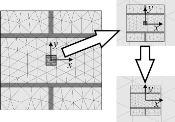
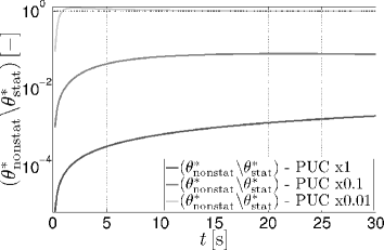
(a)	(b)

Figure 2: (a) Investigated periodic unit cells, (b) resulting evolution of fluctuation temperature

4.2 Influence of macrostructural finite element mesh

One of the concerns of the implementation of FE² scheme is the application of boundary conditions on the macro-scale keeping in mind the scale transition requirement and periodic boundary conditions imposed on the meso-scale. This may become important particularly with a relatively large periodic unit cells which may even exceed the size of macroscopic elements in the vicinity of outer boundary where the macro-elements should be fine enough to ensure a smooth and accurate evolution of driving variables from the outside into the inner parts of a structure.

To address this issue we studied two types of macro-scale discretizations adopted in the two-scale (meso-macro) analysis. The corresponding macro-scale finite element meshes appear in Figs. 3(a),(b). The case when the fine-scale details are assigned to the entire structure is plotted in Fig. 3(c). This mesh, consisting of $7050$ triangular finite elements, served to evaluate the accuracy of the two former discretizations. Fig. 3(a) shows $108$ macro-elements each representing a single meso-problem with assigned periodic boundary conditions, whereas the case in Fig. 3(b) assumes the outer boundary being fully discretized (note that only one-directional flow is considered). There, only the inner part consisting of 72 elements is subject to multi-scale analysis whilst the outer part is modeled as a structure with a real masonry bonding consisting of $3888$ finite elements. A multi-point constrains were introduced to account for an incompatible discretization along the common interface. This latter case is, therefore, expected to heal inaccuracies in the estimation of temperature and moisture fields in the region close to the surface layer.

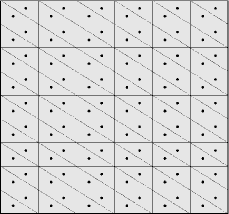
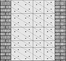
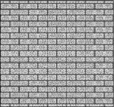
(a)	(b)	(c)

Figure 3: Different finite element representations of masonry wall ($l_{x}=1.92\,\mathrm{[m]}$, $l_{y}=1.80\,\mathrm{[m]}$) - (a) full multi-scale scheme, (b) semi multi-scale scheme, (c) full fine-scale discretization

The following boundary conditions were imposed: on the right-hand side (interior) a constant temperature of $24\,\mathrm{[^{\circ}C]}$ and a constant relative humidity $0.5\,\mathrm{[-]}$ were maintained, while on the left-hand side (exterior) the real climatic data collected over the entire year were prescribed, see Fig. 4.

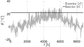
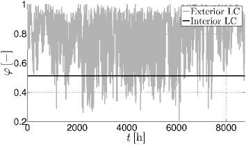
(a)	(b)

Figure 4: Annual loading conditions - (a) temperature, (b) moisture

The results appear in Fig. 5 showing variation of the temperature and moisture along the mid section of the wall after the duration of load of $10$ [h] and $100$ [h], respectively, derived for the macroscopic time step equal to $1$ [h]. Clearly, the notable difference between the exact (full fine-scale discretization) and full multi-scale scheme can be observed in surface layers only and this difference almost disappears with a sufficiently long duration of time. It thus appears that the refined representation of the surface layer through the semi multi-scale scheme, although more accurate compare to full multi-scale scheme, does not bring any particular advantage. This is supported by the calculated average and absolute errors stored in Table 2 taking into account all nodal macroscopic temperatures and moistures in the domain over all time integration steps. Note that for the sake of comparison the fine-scale variables (solution employing the mesh in Fig. 3(c)) were averaged over the cell basically covered by two macro-elements in Fig. 3(a).

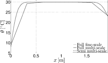
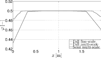
(a)	(b)
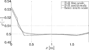
(c)	(d)

Figure 5: Comparison of different macrostructural computations - (a) temperature profile after $t=10\,\mathrm{[h]}$, (b) moisture profile after $t=10\,\mathrm{[h]}$ (c) temperature profile after $t=100\,\mathrm{[h]}$, (d) moisture profile after $t=100\,\mathrm{[h]}$

The presented results thus promote the more accurate semi multi-scale scheme only for calculations demanding higher accuracy of local results especially in initial stages of computation and/or examples with fast changing boundary conditions.

type of comparison	avg. relative error	avg. absolute error
	$[\%]$	$\mathrm{[^{\circ}C]}/[-]$
calculation of temperature
- fine-scale vs. multi-scale	$2.62$	$0.11$
- fine-scale vs. semi multi-scale	$0.71$	$0.03$
calculation of relative humidity
- fine-scale vs. multi-scale	$0.18$	$0.001$
- fine-scale vs. semi multi-scale	$0.05$	$0.001$

Table 2: Averaged relative and absolute errors

4.3 Parallel computation

The essential request by the contractor when studying the mechanical response of Charles Bridge to provide the basis for reconstruction works was a full scale three-dimensional analysis of the bridge. Performing such an analysis in a fully coupled format on a single computer would be computationally unfeasible thus creating the need for a parallel computing. Concentrating on the implementation part of the parallel version of FE² scheme we limit our attention to a two-dimensional section of Charles Bridge subjected, however, to real climatic data displayed already in Fig. 4. Extension to a fully three-dimensional problem is under current investigation and will be presented elsewhere.

As already discussed in the previous section, the present FE² based multi-scale analysis assumes each macroscopic integration point be connected with a certain mesoscopic problem represented by an appropriate periodic unit cell. The solution of a meso-scale problem then provides instantaneous effective data needed on the macro-scale. Such an analysis is particularly suitable for a parallel computing because the amount of transferred data is small. In this regard, the master-slave strategy can be efficiently exploited. To that end, the macro-problem is assigned to the master processor while the solution at the meso-level is carried out on slave processors. At each time step the current temperature and moisture together with the increments of their gradients at a given macroscopic integration point are passed to the slave processor (imposed onto the associated periodic cell), which, upon completing the small scale analysis, sends the homogenized data (effective conductivities, averaged storage terms and fluxes) back to the master processor.

If the meso-scale problems are large enough, the ideal solution is to assign one meso-problem to one slave processor. Clearly, even for very small macro-problems with a few thousands of finite elements, the hardware requirements would be in such a case excessive. On the other hand, if the meso-problems are relatively small, i.e. they contain small number of finite elements, the corresponding analysis might be even shorter than the data transfer between the processors. Then, the computational time associated with the data transfer between the master processor and many slave processors may grow excessively. It is worth mentioning that this time consists of two contributions. The first one represents the latency time (the processors make connection) which is independent of the amount of transferred data whilst the second contribution clearly depends on the amount of data being transferred. For small meso-problems it is therefore reasonable to assign several of them to a single slave processor. The master processor then sends a larger package of data from many macroscopic integration points at the same time to each slave processor so that the latency time does not play a crucial role. This approach was adopted hereinafter.

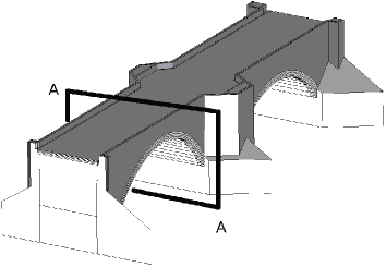
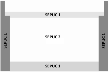
(a)	(b)

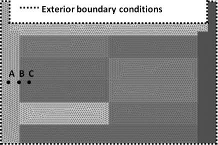
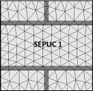
	(d)
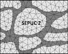
(c)	(e)

Figure 6: (a) Three-dimensional view of Charles Bridge with a two-dimensional A-A section analyzed, (b) Analyzed section showing material regions with assigned meso-scale unit cells, (c) Macrostructural mesh with identified loading conditions and decomposition into sub-domains representing individual slave processors ($l_{x}=10.40\,\mathrm{[m]}$, $l_{y}=6.82\,\mathrm{[m]}$), (d) Mesostructural mesh of regular bonding of masonry (SEPUC 1: $l_{x}=0.45\,\mathrm{[m]}$, $l_{y}=0.44\,\mathrm{[m]}$), (e) Mesostructural mesh of irregular quarry masonry (SEPUC 2: $l_{x}=0.45\,\mathrm{[m]}$, $l_{y}=0.35\,\mathrm{[m]}$).

Fig. 6(a) displays a three-dimensional segment of Charles Bridge examined in the original three-dimensional static calculation [3]. A two-dimensional cut through the mid part of a Charles Bridge arch examined for the parallel computation appears in Fig. 6(b) together with four material regions. These are associated with two heterogeneity systems of the bridge, one representing a regular sand stone masonry of side walls, fence and arches and the other corresponding to an irregular quarry masonry made of arenaceous marl blocks and sand and black lime mortar filling the inner part of the bridge. For simplicity, the bridge deck was assigned the regular pattern. The corresponding periodic unit cells employed for the meso-scale analysis are plotted in Figs. 6(d) and 6(e), respectively.

The finite element mesh used at the macro-level is evident from Fig. 6(c) featuring $7,081$ nodes and $13,794$ triangular elements with a single integration point thus amounting to the solution of $13,794$ meso-problems at each macroscopic time step. This figure also shows decomposition of the macro-problem into $12$ slave processors. The numbers of elements in individual sub-domains being equal to the number of meso-problems handled by the assigned slave processor are listed in Table 3. It should be noted that the assumed decomposition of the macro-problem is not ideal. In comparison with domain decomposition methods, the macro-problem has to be split with respect to the heterogeneity of the material resulting in the variation of number of elements in individual sub-domains between $1046$ and $1748$.

Processor No.	1	2	3	4	5	6	7	8
	9	10	11	12	-	-	-	-
No. of	1218	1748	1046	1052	1214	1210	1052	1054
meso-problems	1046	1052	1054	1048	-	-	-	-

Table 3: Decomposition of the macro-problem into sub-domains.

The number of elements in the two meso-problems amounts to $265$ ($160$ nodes) for SEPUC 1 and to $414$ ($239$ nodes) for SEPUC 2, respectively. Similarly to the macro-problem, the meso-problems have to account for the material heterogeneity. Clearly, the ideal speedup and load balancing are obtained when the decomposition of the macro-problem reflects the meso-problem meshes. However, this is considerably more difficult when compared to the classical mesh decomposition.

The actual analysis was performed on a cluster built at our department. Each node of the cluster is a single processor personal computer Dell Optiplex GX$620$ equipped with $3.54$ GB of RAM. The processors are Intel Pentium with the frequency $3.4$ GHz. The cluster is based on Debian linux $5.0$ and $32$-bit architecture.

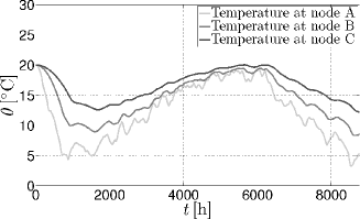
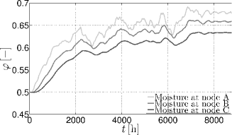
(a)	(b)

Figure 7: Evolution of macroscopic (a) temperature, (b) moisture

Although various mesoscopic heterogeneity patterns were properly accounted for, the material data of individual constituents (bricks or stones and mortar) were taken the same for both the outer and inner part of the bridge, recall Table 1 for specific values. The initial conditions on the macro-scale were set equal to $\varphi=0.5$ [-] and $\theta=20$ [^∘C] and the year round variation of moisture and temperature in Fig. 4 was imposed onto all outer surfaces of the bridge, see Fig. 6(c). Owing to the computational demands the macroscopic time increment was set equal to $10$ [h], which agreed with the real computational time equal to $2.08$ minute for each time step. In view of the results presented in Section 4.2, recall Fig. 5, this justifies, although at the loss of accuracy at the initial stage of computation, the use of full multi-scale scheme. One particular example of the resulting evolutions of macroscopic temperature and moisture at the selected nodes labeled in Fig. 6(c) is seen in Fig. 7.

5 Conclusions

A fully coupled multi-scale analysis of simultaneous heat and moisture transport in masonry structures was implemented in the framework of FE² computational strategy. Two particular issues were addressed: the influence of the finite size of SEPUC when running the transient analysis on both scales and the way of introducing loading on the macro-scale. While the former one plays a significant role in the estimates of macroscopic response, the latter one proves important only in the initial stages of loading.

Special attention was accorded to the implementation of FE² concept in the parallel format employing the master-slave approach. Although not qualitatively fully acceptable, the two-dimensional example of Charles Bridge raised a number of questions to the solution efficiency particularly with reference to a proper subdivision of the analyzed macro-domain and local finite element mesh of individual meso-scale SEPUCs. The present findings summarized in Section 4.3 will be utilized in a fully three-dimensional analysis being the subject of our current research effort.

Appendix A

The list of material parameters to be obtained experimentally are stored in Table 1. The transport coefficients that enter Eqs. (1) and (2) are provided by

• $w$ - water content $\mathrm{[kgm^{-3}]}$,

  $$w=w_{f}\frac{(b-1)\varphi}{b-\varphi},$$ (16)

  where $w_{f}$ is the free water saturation and $b$ is the approximation factor, which must always be greater than one. It can be determined from the equilibrium water content ($w_{80}$) at $0.8$ [-] relative humidity by substituting the corresponding numerical values in equation (16).

• $\delta_{p}$ - water vapor permeability $\mathrm{[kgm^{-1}s^{-1}Pa^{-1}]}$,

  $$\delta_{p}=\frac{\delta}{\mu},$$ (17)

  where $\mu$ is the water vapor diffusion resistance factor and $\delta$ is the vapor diffusion coefficient in air $\mathrm{[kgm^{-1}s^{-1}Pa^{-1}]}$ given by

  $$\delta=\frac{2.306\cdot{}10^{-5}\,p_{a}}{R_{v}\,(\theta+273.15)\,p}\left(\frac{\theta+273.15}{273.15}\right)^{1.81},$$ (18)

  with $p$ set equal to atmospheric pressure $p_{a}=101325$ [Pa] and $R_{v}$ = $R$/$M_{w}=461.5$ [$\mathrm{Jkg^{-1}K^{-1}}$]; $R$ is the gas constant ($8314.41$ [Jmol^-1K^-1]) and $M_{w}$ is the molar mass of water ($18.01528$ [kgmol^-1]).

• $D_{\varphi}$ - liquid conduction coefficient $\mathrm{[kgm^{-1}s^{-1}]}$,

  $$D_{\varphi}=D_{w}\frac{\mathrm{d}w}{\mathrm{d}\varphi},$$ (19)

  where $D_{w}$ is the capillary transport coefficient given by

  $$D_{w}=3.8\left(\frac{A}{w_{f}}\right)^{2}\cdot{}10^{3w/(w_{f}-1)},$$ (20)

  where the derivative of the moisture storage function $\displaystyle{\frac{\mathrm{d}w}{\mathrm{d}\varphi}}$ is obtained by differentiating Eq. (16).

• $\lambda$ - thermal conductivity $\mathrm{[Wm^{-1}K^{-1}]}$,

  $$\lambda=\lambda_{0}\left(1+\frac{b_{\mathrm{tcs}}w}{\rho_{s}}\right),$$ (21)

  where $\lambda_{0}$ is the thermal conductivity of dry building material, $\rho_{s}$ is the bulk density and $b_{\mathrm{tcs}}$ is the thermal conductivity supplement.

• $p_{\mathrm{sat}}$ - water vapor saturation pressure $\mathrm{[Pa]}$,

  $$p_{\mathrm{sat}}=611\,\exp\left(\frac{a\,\theta}{\theta_{0}+\theta}\right),$$ (22)

  where

  $$\begin{array}[]{ccc}a=22.44&\theta_{0}=272.44\,[^{\circ}\mathrm{C}]&\theta<0\,[^{\circ}\mathrm{C}]\\[14.22636pt] a=17.08&\theta_{0}=234.18\,[^{\circ}\mathrm{C}]&\theta\geq 0\,[^{\circ}\mathrm{C}]\end{array}$$ (23)

• $h_{v}$ - evaporation enthalpy of water $\mathrm{[Jkg^{-1}]}$

  $$h_{v}=2.5008\cdot{}10^{6}\left(\frac{273.15}{\theta}\right)^{(0.167+3.67\cdot{}10^{-4}\theta)}.$$ (24)

References

- [1] H. M. Künzel, K. Kiessl, Calculation of heat and moisture transfer in exposed building components, International Journal of Heat and Mass Transfer 40 (1997) 159–167.
- [2] R. Přikryl, A. Št́astná, Contribution of clayey-calcareous silicite to the mechanical properties of structural mortared rubble masonry of the medieval Charles Bridge in Prague (Czech Republic), Engineering Geology 115 (3–4) (2010) 257–267. doi:10.1016/j.enggeo.2010.06.009.
- [3] J. Novák, J. Zeman, M. Šejnoha, J. Šejnoha, Pragmatic multi-scale and multi-physics analysis of Charles Bridge in Prague, Engineering Structures 30 (11) (2008) 3365–3376.
- [4] Charles bridge IS. the information system based on Charles Bridge reconstruction research, http://iskarluvmost.fsv.cvut.cz/homepage/.
- [5] J. Sýkora, M. Šejnoha, J. Šejnoha, Homogenization of coupled heat and moisture transport in masonry structures including interfaces, Applied Mathematics and Computation 0 (2011) 0–0. doi:10.1016/j.amc.2011.02.050.
- [6] R. Valenta, M. Šejnoha, J. Zeman, Macroscopic constitutive law for mastic asphalt mixtures from multiscale modeling, International Journal for Multiscale Computational Engineering 8 (1) (2010) 131–149.
- [7] M. Šejnoha, J. Vorel, R. Valenta, J. Zeman, Virtual experiments and statistically equivalent rves towards macroscopic constitutive laws, in: B. Topping (Ed.), Proceedings of the The Thirteenth International Conference on Civil, Structural and Environmental Engineering Computing, Chania, Crete, Greece 6-9 September 2011, Civil-Comp Press, 2011.
- [8] F. Larsson, K. Runesson, F. Su, Variationally consistent computational homogenization of transient heat flow, International Journal for Numerical Methods in Engineering 81 (2010) 1659–1686.
- [9] R. Černý, P. Rovnaníková, Transport Processes in Concrete, London: Spon Press, 2002.
- [10] J. Sýkora, J. Vorel, T. Krejčí, M. Šejnoha, J. Šejnoha, Analysis of coupled heat and moisture transfer in masonry structures, Materials and Structures 42 (8) (2009) 1153–1167.
- [11] H. M. Künzel, Simultaneous Heat and Moisture Transport in Building Components, Tech. rep., Fraunhofer IRB Verlag Stuttgart (1995).
- [12] O. Krischer, W. Kast, Die wissenschaftlichen Grundlagen der Trocknungstechnik, Dritte Auflage, Berlin: Springer, 1978.
- [13] K. Kiessl, Kapillarer und dampfförmiger feuchtetransport in mehrschichtlichen bauteilen, Ph.D. thesis, Universität in Essen (1983).
- [14] J. Sýkora, Multiscale modeling of transport processes in masonry structures, Ph.D. thesis, Czech Technical University in Prague (2010).
- [15] J. Zeman, M. Šejnoha, From random microstructures to representative volume elements, Modelling and Simulation in Materials Science and Engineering 15 (4) (2007) S325–S335.
- [16] I. Özdemir, W. A. M. Brekelmans, M. G. D. Geers, Computational homogenization for heat conduction in heterogeneous solids, International Journal for Numerical Methods in Engineering (2) (2008) 185 –204.
- [17] M. Pavlíková, Z. Pavlík, R. Černý, Hygric and thermal properties of materials of historical masonry, in: Proceedings of the 8th Symposium on Building Physics in the Nordic Countries, 2008.