Steps Toward a Theory of Visual Information:
 
Active Perception, Signal-to-Symbol Conversion
and the Interplay Between Sensing and Control

Preface

This manuscript has been developed starting from notes for a summer course at the First International Computer Vision Summer School (ICVSS) in Scicli, Italy, in July of 2008. They were later expanded and amended for subsequent lectures in the same School in July 2009. Starting on November 1, 2009, they were further expanded for a special topics course, CS269, taught at UCLA in the Spring term of 2010.

I acknowledge contributions, in the form of discussions, suggestions, criticisms and ideas, from all my students and postdocs, especially Andrea Vedaldi, Paolo Favaro, Ganesh Sundaramoorthi, Jason Meltzer, Taehee Lee, Michalis Raptis, Alper Ayvaci, Yifei Lou, Brian Fulkerson, Teresa Ko, Daniel O’Connor, Zhao Yi, Byung-Woo Hong, Luca Valente.

In addition to my students, I am grateful to my colleagues Ying-Nian Wu, Andrea Mennucci, Anthony Yezzi, Veeravalli Varadarajan, Peter Petersen, and Alessandro Chiuso for discussions leading to many of the insights described in this manuscript. I also wish to acknowledge discussions with Joseph O’Sullivan, Richard Wesel, Alan Yuille, Serge Belongie, Pietro Perona, Jitendra Malik, Ruzena Bajcsy, Yiannis Aloimonos, Sanjoy Mitter, Roger Brockett, Peter Falb, Alan Willsky, Michael Jordan, Judea Pearl, Deva Ramanan, Charless Fowlkes, Giorgio Picci, Sandro Zampieri, Lance Williams, George Pappas, Tyler Burge, James Clark, Jan Koenderink, Yi Ma, Olivier Faugeras, John Tsotsos, Tomaso Poggio, Allen Tannenbaum, Alberto Pretto. I wish to thank Andreas Krause, Daniel Golovin, Andrea Censi, Lorenzo Rosasco, Max Welling and Taco Cohen for many useful comments and corrections. Finally, I wish to thank Roberto Cipolla, Giovanni Farinella and Sebastiano Battiato for organizing ICVSS that has initiated this project.

The work leading to this manuscript was made possible by guidance, encouragement, and generous support of three federal research agencies, under the leadership of their Program Managers: Behzad Kamgar-Parsi of ONR, Liyi Dai of ARO, and Fariba Fahroo of AFOSR. Their help in making this project happen is gratefully acknowledged. I also wish to acknowledge discussion and feedback from Tristan Nguyen, Alan Van Nevel, Gary Hewer, William McEneany, Sharon Heise, and Belinda King.

Note from 2017: Much of this work is superseded and distilled in the 2017 paper “Emergence of Invariance and Disentanglement in Deep Representations”, [1].

Chapter 1 Preamble

“Intelligent Behavior” is often assumed to involve some sort of “internal representation” made of discrete “symbols.” However, the Data Processing Inequality suggests that such a signal-to-symbol conversion is detrimental to the optimality of decision and control actions downstream. This opens a number of questions that motivate this manuscript. Readers uninterested in such philosophical issues can skip this section.

Perceptual agents, from plants to humans, measure samples of physical processes (“signals”) that are essentially continuous. They also perform actions in the continuum of physical space. And yet, cognitive science, epistemology, and in general modern philosophy associate “intelligent behavior” with some kind of “internal representation” built upon discrete symbols (e.g. “concepts”, “ideas”, “objects”, “categories”) that can be manipulated and inferred with logic and probabilistic inference. But why should such a “signal-to-symbol” conversion occur? How does it yield an evolutionary advantage? What principles should guide it?

Information Theory suggests that such a signal-to-symbol conversion may be counter-productive: If we consider biological systems as machines that perform actions or make decisions in response to stimuli in a way that maximizes some decision or control objective, then the Data Processing Inequality indicates that the best possible agents would avoid data analysis, i.e., the process of breaking down signals into discrete entities or symbols. These considerations apply regardless of the specific control or decision task, from the simplest binary decision (e.g. “is a specific object present in the scene?”) to the most complex (e.g. “survival”).

So, why would we need, or even benefit from, an internal representation? Is “intelligence” not possible in an “analog” setting? Or is data analysis necessary for cognition? If so, what would be the mathematical and computational principles that guide it? What if the task is not known; is a notion of representation still meaningful in the absence of a task?

In the fields of Signal Processing, Image Processing, and Computer Vision, we routinely torture the data (filtering, sampling, anti-aliasing, edge detection, feature selection, segmentation, etc.), seemingly against the basic tenets of Information and Decision Theory. The Data Processing Inequality would instead suggest an approach whereby data are fed directly into a “black-box” decision or control machine designed to optimize a (possibly very complex) cost functional.

One could argue that data analysis in biological systems is not guided by any optimality principle, but an accident due to the constraints imposed by biological hardware. In [180], Turing showed that (continuous) reaction-diffusion partial differential equations (PDEs) that govern ion concentrations in neurons exhibit discrete/discontinuous solutions. This may explain “spikes” in neuronal signals and perhaps from there symbols. But if we want to build machines that interact intelligently with their surroundings and are not bound by the constraints of biological hardware, should we draw inspiration from biology, or can we do better by following the principles of Information Theory?

The question of existence of an “internal representation” is best framed within the scope of a task, which provides a falsifiability mechanism. In the context of visual analysis I distinguish four broad classes of tasks, which I call the four “R’s” of vision: Reconstruction (building models of the geometry, or shape, of the scene), Rendering (building models of the photometry, or material properties, of the scene), Recognition and other vision-based decisions such as detection, localization, categorization and more in general scene semantics, and Regulation or, more in general, vision-based control such as tracking, navigation, obstacle avoidance, manipulation etc..

In this manuscript, we will explore the issue of representation from visual data for decision and control tasks. To avoid philosophical entanglements, we will not attempt to define “intelligent behavior” or even “knowledge,” other than to postulate that knowledge – whatever it is – comes from data, but it is not data. This leads to the notion of the “useful portion” of the data, which one might call “information.” So, our first step will be a definition of what “information” means in the context of performing a decision or action based on sensory data.

As we will see, visual perception plays a key role in the signal-to-symbol barrier. As a result, much of this manuscript is about vision. Specifically, the need to perform decision and control tasks in a manner that is independent of nuisance factors including scaling and occlusion phenomena require the perceptual agent (or, more in general, its evolved species) to exercise control over certain aspects of the sensing process. This inextricably ties sensing, information and control. A case-in-point is provided by Sea Squirts, or Tunicates, shown in Figure 1.1. These are organisms that possess a nervous system (ganglion cells) and the ability to move. They spend part of their lives as predators, but eventually settle on a rock, become stationary and thence swallow their own brain. Scaling and occlusion play a critical role: The first makes the continuum limit relevant, the second makes control a critical element in the analysis. These are present in a number of remote sensing modalities, including optical, infrared, multi-spectral imaging, as well as active ranging such as radar, lidar, time-of-flight, etc.

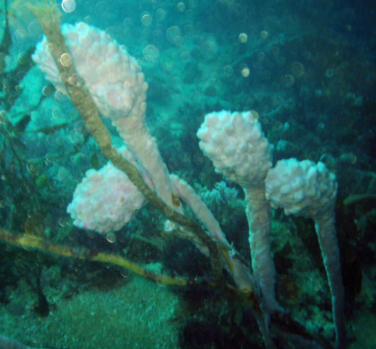
Figure 1.1: The Sea Squirt, or Tunicate, is an organism capable of mobility until it finds a suitable rock to cement itself in place. Once it becomes stationary, it digests its own cerebral ganglion cells, or “eats its own brain,” and develops a thick covering, a “tunic” for self defense.⁶

1.1 How to read this manuscript

This manuscript is designed to allow different levels of reading. Some of the material requires some background beyond calculus and linear algebra. To make the manuscript self-contained, basic elements of topology, variational methods and optimization, image processing, radiometry, etc. are provided in a series of appendices. These are color coded. The parts of the main text that require background in the corresponding discipline are coded with the same color. The reader can then either read through the colored text if he or she is familiar with that subject, disregarding the appendices, or use the appendix as a reference in case he or she is not familiar with the subject, or skip the colored text altogether. The manuscript is structured to allow getting the “big picture” without any mathematical formalism by just reading the black text.

Summary for the experts (to be skipped by others)

This section summarizes the content of the manuscript in a succinct manner. It can be used as a summary, or as a reference to the broader picture while reading the rest of the manuscript. For most readers, this summary will be cryptic or confusing at a first reading. If it was otherwise, there would be no need for a manuscript to follow.

What makes vision difficult, and might explain the fact that almost half of the primate brain is devoted to it [57, 143], is the fact that nuisance factors in the data formation process account for almost all the complexity of the data [167]. Such factors include invertible nuisances such as contrast and viewpoint (away from occlusions), and non-invertible ones such as occlusions, quantization, noise, and general illumination changes. After discounting the effects of the nuisances in the data (invariance), even if one had started with infinite-resolution data, what is left is “thin” (supported on a zero-measure subset of the image domain). The complexity of the data after the effects of invertible nuisances has been remove is called Actionable Information. The fact that Actionable Information can be thin in the data is relevant to the signal-to-symbol barrier problem.

How can we deal with nuisances? At decision time one can marginalize them (Bayes) or search for the ones that best explain the data (max-out, or maximum-likelihood). Some, however, may be eliminated in a process called canonization. While marginalization and max-out require solving complex integration or optimization problems at decision time, canonization can be pre-computed, and hence it enables straight comparison of statistics at decision time. It is preferable if time-complexity is factored in. However, this benefit comes with a predicament, in that canonization cannot decrease the expected risk, but at best leave it unchanged. Among the statistics that leave the risk unchanged (sufficient statistics), the ones that are also invariant to the nuisances would be the ideal candidates for a representation: They would contain all and only the functions of the data that matter to the task.

Unfortunately, while for invertible nuisances one can construct complete features (invariant sufficient statistics), that act as a lossless representation, occlusion and quantization are not invertible. Thus, there is a gap between the maximal invariant and the minimal sufficient statistics. This gap cannot, in general, be filled by processing passively gathered data.

However, when one can exercise control on the sensing process, then some non-invertible nuisances can become invertible. Occlusions can be inverted by moving around the occluder. Scaling/quantization can be inverted by moving closer. Even the effects of noise can be countered by increasing temporal sampling and performing suitable averaging operations. Therefore, in an active sensing scenario one can construct representations that are (asymptotically) lossless for decision and control tasks, and yet have low complexity relative to the volume of the raw data. This inextricably ties sensing and control. It also may enable achieving provable bounds, by generalizing Rate-Distortion theory to Perception-Control tradeoffs, whereby the “amount of control authority” over the sensing process (to be properly defined) trades off the expected error in a visual decision task.

In this manuscript, we characterize representations as complete invariant statistics, and call hallucination the simulation of the data formation process starting from a representation (as opposed to the actual scene). We define Actionable Information as the complexity of the maximal invariant statistics of the data, and Complete Information as the complexity of the (minimal sufficient statistic of a) complete representation. We define co-variant detectors, that enable the process of canonization, and their associated invariant descriptors. We define canonizability, and address the following questions: (i) When is a classifier based on an invariant descriptor optimal? (in the sense of minimizing the expected risk) (ii) what is the best possible descriptor? (iii) what nuisances are canonizable? (and therefore can be dealt with in pre-processing, as opposed to having to be marginalized or max-outed at decision time).

Four concepts introduced in this study are key to the analysis and design of practical systems for performing visual decision and control tasks: Canonizability, Commutativity, Structural Stability, and Proper Sampling.

Canonization is not sufficient to infer a complete representation, unless nuisances commute with one another. We show that the only nuisance that is canonizable and commutative is the isometric group of the plane. Affine transformations in general, and the scale group in particular, should not be canonized, but should instead be sampled and marginalized.

Canonizing functionals, designed to select an element of the canonizable nuisance group, should be stable with respect to variations of the non-canonizable nuisances. We introduce the notion of Structural Stability, that is related to catastrophe theory and persistent topology. Selection by maximum structural stability margins gives rise to a novel feature selection scheme [106].

Whether the structure detected by a canonizing functional is “real” (i.e. it arises from phenomena in the scene) or an “alias” (i.e. it originates from artifacts of the image formation process, for instance quantization) depends on whether the signal is properly sampled. We introduce a notion of proper sampling that, unlike traditional (Nyquist-Shannon) sampling, cannot be decided based on a single datum (one image snapshot), but instead requires multiple images. This notion gives rise to a novel feature tracking scheme [106].

Intra-class variability can be captured by endowing the space of representations (which are discrete entities) with a probabilistic structure and learning distributions of individual objects or parts, clustered by labels. Objects are not necessarily rigid/static, but can also include “actions” or “events” that unravel in time. Time can be treated as yet another nuisance variable, which unfortunately is not invertible and therefore cannot be canonized without a loss. Time is, therefore, best dealt with by marginalization or max-out at decision time [148].

Along the way in our investigation we also discuss the role of “textures” and their dual (“structures”), and characterize them as the complement of canonizable regions [23].

1.2 Related literature

The design and computation of visual representations for recognition has a long history (see [118, 170] and references therein). While Marr’s representation using zero-crossings of differential operators was discredited because of instability in the reconstruction process (i.e. obtaining images back from their representations), reconstructing images is not necessarily the purpose, if a representation is to support decision and control tasks. Many have attempted to design representations that are tailored to recognition (as opposed to image reconstruction) tasks, some using similar ideas of extrema of scale-spaces constructed from differential operators [114, 109]. However, most of these designs have been performed in an ad-hoc manner, guided by intuition, common sense, and some biological inspiration. Statistical decision theory would instead call for the direct design of general “super-classifiers” forgoing intermediate representations altogether, unless directly tied to the task.

Our earlier work [162] aims to frame the construction of invariant/sufficient representations in the context of Active Vision, formalizing some ideas of J. J. Gibson [65]. Gibson’s approach, however, falls short on several counts. First, invariance is too much to ask. In the process of being invariant to general viewpoints, shape becomes indiscriminative [186]. And yet, we know we can discriminate objects that are deformed versions of the same material. Second, often priors are available, from training or otherwise, both on the nuisance and on the class, and such priors should be used. There is no point in requiring invariance to illuminations that will never be; better instead to be insensitive to common nuisances, and relax the representation where nuisances have low probability even though this opens the possibility of illusions for unlikely nuisance and scene combinations (Fig. 1.2).

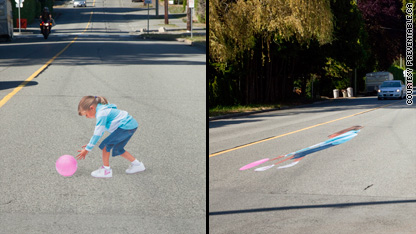
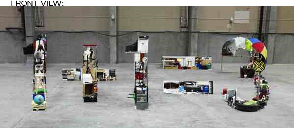
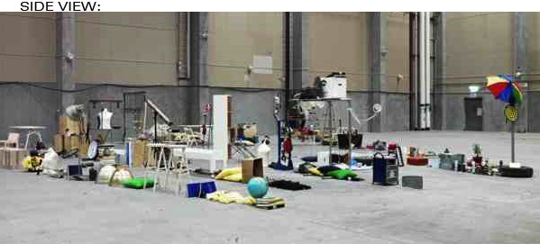
Figure 1.2: In the absence of sufficiently informative data (e.g., one image), priors enable classification that, occasionally, can be incorrect if the nuisances and scene concur to form a visual illusion. The scene on the top-left looks like a girl picking up a ball (image courtesy of Preventable.com), rather than a flat painting on the road surface. Similarly, the purposeful collection of objects on the bottom looks like meaningful symbols when seen from a carefully selected (non-accidental) vantage point.

Third, even though the Active Vision paradigm is appealing, in practice we often do not have control on the sensing platform.

Therefore, there remains the need to properly treat nuisances that are non-invertible, such as occlusions, quantization and noise, in a passive sensing scenario, and to be able to exploit priors when available.

The recent literature is studded with different approaches for low-level pre-processing of images for visual classification. These include various feature detectors and descriptors, too many to cite extensively, but the most common being [114, 127]. These are compared empirically on end-to-end tasks such as wide-baseline matching [127], categorization [107], or category localization and segmentation [122] tasks. However, an empirical evaluation tells us which scheme performs better, but gives us no indication as to the relation between different schemes, no hint on how to improve them, and no bounds on the best achievable performance that can be extrapolated to other datasets with provable guarantees.

Therefore, there remains the need to develop a framework for the analysis and design of feature detectors/descriptors, that allows rational comparison of existing descriptors, and engineering design of new ones, and understanding of the conditions under which they can be expected to perform.

There is a sizable literature on the detection and computation of structures in images. In particular, [171] derive detectors based on a series of axioms and postulates. However, while these explain how such low-level representations should be constructed, they give no indication as to why they would be needed in the first place. Much of the motivation in this literature stems from biology, and in particular the structure of early stages of processing in the primate visual system.

By its nature, this manuscript relates to a vast body of literature in low-level vision and also Active Vision [4, 15]. Ideally it relates to every paper, by providing a framework where different approaches can be understood and compared. However, it is possible that some approaches may not fit into this framework. I hope that this work provides a seed that others can grow or amend.

This manuscript also lends some analytical support for the notion of embodied cognition that has been championed by cognitive roboticists and philosophers including [29, 103, 183, 140, 123, 15].

Finally, the work of Naftali Tishby and co-workers, starting from [173], has been addressing similar questions using an information-theoretic framework; work is underway to combine and reconcile the two approaches.

Chapter 2 Formalizing Visual Decisions

Visual classification tasks – including detection, localization, categorization, and recognition of general object classes in images and video – are challenging because of large in-class variability. For instance, the class “chair”, defined as “something you can sit on” (presumably man-made), comprises a diversity of shapes, sizes and materials that result in a wide variety of images (Figure 2.1).

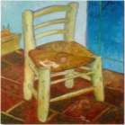
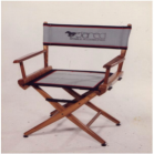
$I_{1}$ $I_{2}$ $\ldots$ $I_{n}$ similar shape? similar appearance? similar function? ??

Figure 2.1: Category recognition: Given images $\{I_{1},\dots,I_{n}\}$ of scenes that belong to a common class (left), does a new image $\tilde{I}$ (right) portray a scene that belongs to the same class?

Even if one sets aside within-class variability and considers the detection, localization or recognition of an individual object (e.g. this chair) from a field of alternate hypotheses (e.g. other chairs), the data still exhibits large variability due to nuisance factors such as viewpoint, illumination, occlusion, etc., that have little to do with the identity of the object (Figure 2.2).

It is tempting to hope that a powerful classifier fed with raw data could be trained to, somehow, discard the variability in images due to nuisance factors, and reliably recognize object, their classes and relations in pictures. The results in [166] suggest otherwise, since the volume of the quotient of the set of images modulo changes of viewpoint and contrast is infinitesimal relative to the volume of the data. This means that a hypothetical classifier fed with raw images would spend almost all of its resources learning the nuisance variability, rather than the intrinsic variability of objects of interest. This is realistic at the phylogenic (at the evolutionary time scale), but not at the individual (ontogenic) level. This would hold a-fortiori once complex illumination phenomena, occlusions, and quantization – all neglected in [166] – were factored in.

Moreover, if one’s training consists of individual images each of a different scene, as in Fig. 2.1, the process is even more problematic as a single image does not afford the ability of disentangling nuisance variability from intrinsic variability, and the complexity of the scene is infinitely more complex than the complexity of (even infinitely many) images. Therefore, a hypothetical learning machine fed with however large a dataset of individual images, each of a different scene, would never even learn that there is a scene, with shape, reflectance, illumination, etc. but instead just learn patterns of intensity in the images.

It is equally tempting to hope that one could pre-process the data to obtain some “features,” that do not depend on these nuisances, and yet retain all the “information” present in the data. Indeed, [166] suggests a construction of such features that, however, requires nuisances to have the structure of a group and hence breaks down in the presence of complex illumination effects, occlusions and quantization. One could relax such strict “invariance” requirement to some sort of “insensitivity” but, in general, pre-processing can only reduce the performance of any classifier downstream [156]. This brings into question the role of “vision-as-pre-processing for general-purpose machine learning.” Why should one perform segmentation, edge detection, feature selection and other generic low-level vision (pre-processing) operations, if the classification performance decreases?

This goes to the heart of a notion of “information.” Ideally, the purpose of vision would be to “extract information” from images, where “information” intuitively relates to whatever portion of the data “matters” in some sense. Traditional Information Theory has been developed in the context data transmission, where one wants to reproduce as faithful as possible a copy of the data emitted by the source, after it has been corrupted by the channel. Thus the goal is reproduction (or reconstruction) of the data, with minimal distortion, and the “representation” simply consists of a compressed encoding of the data that exploits statistical regularity. In this context, every bit counts, and the semantic aspect of information is indeed irrelevant, as Shannon famously wrote. The theory yields a tradeoff between the minimum size of the representation as a function of the maximum amount of distortion. This tradeoff is computed explicitly for very simple cases (e.g. the memoryless Gaussian channel), but nevertheless the general formulation of the problem is one of Shannon’s most significant achievements.

In our context, the data (images) are to be used for decision purposes (detection, localization, recognition, categorization). The goal is to minimize risk. In this context, there may be conditions where most of the data is useless, and the semantic aspect is fundamental, for the sufficient statistics can be discrete (symbols) even when the data lives in the continuum.

Several have advocated the development of a theory, mirroring Shannon’s Rate-Distortion Theory, to describe the minimum requirements (in terms of size of the representation, computational or other “cost”) in order to have a recognition error that is bounded above. Ideally, like in Shannon’s case, this bound could be made arbitrarily small by paying a high-enough price. Despite many efforts, no theory has emerged, only special cases restricted to imaging modalities where some of the crucial aspects of image formation (scaling and occlusions) are not manifest. This may not be by chance because, in the context of visual recognition, the worst-case scenario is an arbitrarily high error rate. This is not surprising, and indeed can be considered trivial. What may be a bit more surprising is that even the average-case scenario can be arbitrarily bad, as we will argue in Section LABEL:sect-passive-bounds. This may also shed some light on the limitations of benchmark datasets, if the performance of a given algorithm is interpreted as representative of performance on other datasets. The result of the benchmarking are meaningful to the extent in which the dataset is representative of the scenarios one wishes to capture, but no guarantee can be made on the generalization properties of these methods. Again, scale, quantization and occlusion conjure towards the failure of any “passive” recognition scheme to provide generalization bounds. What is surprising is that, if the data acquisition process can be controlled, then both the worst-case and average-case error can be bounded, and indeed they can be made (asymptotically) arbitrarily small (Section LABEL:sect-active-bounds). Analogously to Shannon’s Rate-Distortion theory, there is a tradeoff between the “control authority” one can exercise over the sensing process, and the performance in a decision task (Section LABEL:sect-control-recognition).

In the next section, we begin the formalization process necessary to answer some of the questions raised so far. For the purpose of simplicity, we will reduce visual perception to a collection of classification tasks, which is admittedly restrictive, but sufficient to commence formalization.

2.1 Visual decisions as classification tasks

By “visual decision” we mean tasks such as detection, localization, categorization and recognition of objects in images or video. These are all classification problems, where in some cases the class is a singleton (recognition), in other cases it can be quite general depending on functional or semantic properties of objects (Figure 2.1). Conceptually, they all require the evaluation and learning of the likelihood of the data (one or more images $I$) given the class label $c$: $p(I|c)$. To simplify the narrative, we consider binary classifiers $c\in\{0,1\}$ with equal prior probability $P(c)=\frac{1}{2}$. Generalizations are conceptually, although not computationally, straightforward.

A decision rule, or a classifier, is a function $\hat{c}:{\cal I}\rightarrow\{0,1\}$ mapping the set of images onto labels. It is designed to keep the average loss from incorrect decisions small. A loss function $\lambda:\{0,1\}^{2}\rightarrow\mathbb{R}^{+};(\hat{c},c)\mapsto\lambda(\hat{c},c)$ maps two labels to a positive real value. We will consider, for simplicity, the symmetric $0-1$ loss, where $\lambda(\hat{c},c)=1-\delta(\hat{c},c)$, where $\delta$ is Kronecker’s delta, that is $1$ if the labels are the same, $0$ if they are different. The average loss, a.k.a. conditional risk, is given by

$$R(I,\hat{c})=\sum\lambda(\hat{c},c)P(c|I).$$ (2.1)

It can be shown [53] that the decision rule that minimizes the conditional risk, that is

$$\hat{c}=\hat{c}(I)\doteq\arg\min_{c}R(I,c)$$ (2.2)

is optimal in the sense that it minimizes the expected (Bayesian) risk

$$R(c)\doteq\int R(I,c)dP(I).$$ (2.3)

That is, if one could actually compute this quantity, which depends on the availability of the probability measure $dP(I)$, which is tricky to even define, let alone learn and compute [130]. However, in the context of our investigation this is irrelevant: Whatever mathematical object $dP(I)$ is, we can easily sample from it by simply capturing images $I\sim dP(I)$, as we will see in Section 8. We will see in Section 3.1 that, even to generate “simulated images,” we do not need access to the “true” distribution $dP(I)$, but rather to a representation, which we will define in Section 3 and discuss in Section 3.1.

Under the assumptions made, minimizing the conditional risk is equivalent to maximizing the posterior $p(c|I)$, which in turn (under equiprobable priors $P(c=1)=P(c=0)=1/2$) is equivalent to maximizing the likelihood $p(I|c)$:

$$\boxed{\hat{c}=\arg\max_{c\in\{0,1\}}p(I|c).}$$ (2.4)

So, in a sense, the problem of visual decision-making, including detection, localization, recognition, categorization, is encapsulated in (2.4). That would be easy enough to solve if we could actually compute the likelihood.

The difficulty in visual decision problems arises from the fact that the image $I$ depends on a number of nuisance factors that do not depend on the class, and yet they affect the data. What is a nuisance depends on the task, and may include viewpoint, illumination, partial occlusions, quantization etc. (Figure 2.2). If we could, we would base our decision not on the data $I$, but on hidden variables $\xi$ that comprise the defining characteristics of the scene (object, category, location, event, activity etc.) that depend on the class $c$, through a Markov chain $c\rightarrow\xi\rightarrow I$. This would correspond to a data generation model whereby a sample $c$ is selected from $P(c)$, based on which a sample $\xi$ is selected from $dQ_{c}\doteq dP(\xi|c)$, from which a measurement $I$ is finally sampled via an image-formation functional $I=h(\xi)$.

However, because of the nuisances, we have to instead consider a generative model of the form $I=h(\xi,\nu)$, where $h$ is a functional that depends on the imaging device and $\nu$ are all the nuisance factors. It is convenient to isolate within the nuisance $\nu$ the additive noise component $n$ arising from the compound effects of un-modeled uncertainty, although there is no added generality as $n$ can be subsumed in the definition of $\nu$. It is also useful to isolate the nuisances that act as a group on the scene, $g$, although again we could lump them into the definition of $\nu$. If we model explicitly the group and the noise, we have a model of the form

$$\boxed{I=h(g,\xi,\nu)+n}$$ (2.5)

This is the formal model that we will adopt throughout the manuscript (Figure 2.2). In the next section we make this formal notation a bit more precise with a specific instantiation, the so-called Ambient-Lambert model. More realistic instantiations are described in Appendix B.1. The reader interested in generalizations of the simple symmetric binary decision case can consult any number of textbooks, for instance [53].

$I=h(\xi,\nu)$

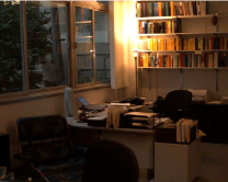
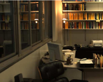
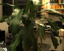
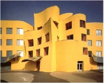
$\tilde{I}=h(\xi,\tilde{\nu}),~{}~{}\tilde{\nu}=$ illumination $\tilde{\nu}=$ viewpoint $\tilde{\nu}=$ visibility $\tilde{I}=h(\tilde{\xi},\tilde{\nu}),~{}~{}\tilde{\xi}\neq\xi$

Figure 2.2: The same scene $\xi$ can yield many different images depending on particular instantiations of the nuisance $\nu$.

2.2 Image formation: The image, the scene, the nuisance, and the Lambert-Ambient (LA) Model

Figure 2.3: Image-formation model: The scene is described by objects whose geometry is represented by $S$ and photometry (reflectance) $\rho$. The image, taken from a camera moving with $g$, is obtained by a central projection onto a planar domain $D$, and a contrast transformation.

In this section, that can be skipped at first reading, we instantiate the formal notation (2.5) for a simple model used throughout the manuscript. All the symbols used, together with their meaning, are summarized for later reference in Appendix C in the order in which they appear. This section is necessary to make the formal notation above meaningful. However, its content will actually not be used until Sections 3.1, 3.4, and will be exploited in full only starting in Section 4. Therefore, the reader can skip this section at first reading, and come back to it, or to Appendix C, as needed. The model we introduce in this section is the simplest instantiation of (2.5) that is meaningful in the context of image analysis. More sophisticated models, and their relation to the simplest one introduced here, are described in Appendix B.1.

An image $I:D\subset\mathbb{R}^{2}\rightarrow\mathbb{R}_{+}^{k};\ x\mapsto I(x)$ is a positive-valued map defined on a planar domain $D$; we will focus on gray-scale images, $k=1$, but extensions to color $k=3$ or multiple spectral bands can be made. The scene, indicated formally by $\xi=\{S,\rho\}$, is described by its shape $S$ and reflectance (albedo) $\rho$. The shape component $S\subset\mathbb{R}^{3}$ is described by piecewise smooth surfaces. The surface $S$ does not need to be simply connected, and can instead be made of multiple connected components, $S_{i}$, with $\cup_{i}S_{i}=S$, each representing an object. The reflectance $\rho$ is a function defined on such surfaces, with values in the same space of the range of the image, $\rho:S:\rightarrow\mathbb{R}^{k}$. In the presence of an explicit illumination model, $\rho$ denotes the diffuse albedo of the surface. In the absence of an illumination model, one can think of the surfaces as “self-luminous” and $\rho(p)$ denotes the energy emitted by an infinitesimal area element at the point $p$ isotropically in all directions. We call the space of scenes $\Xi$. Deviations from diffuse reflectance (inter-reflection, sub-surface scattering, specular reflection, cast shadows) will not be modeled explicitly and lumped as additive errors $n$.

Nuisance factors in the image-formation process are divided into two components, $\{g,\nu\}$, one that has the structure of a group $g\in G$, and a component that is not a group, e.g. quantization, occlusions, cast shadows, sensor noise etc. We denote the image-formation model formally with a functional $h$, so that $I=h(g,\xi,\nu)+n$ as in (2.5). This highlights the role of group nuisances $g$, the scene $\xi$, non-invertible nuisances, and the additive residual that lumps together all unmodeled phenomena including noise and quantization (non-additive noise phenomena can be subsumed in the non-invertible nuisance $\nu$). We often refer to the group nuisances as invertible and the non-group nuisances as non-invertible.

The simplest instantiation of this model is the so-called Lambert-Ambient-Static (LAS) model, that approximates a static Lambertian scene seen under constant diffuse illumination, describing reflectance via a diffuse albedo function and thus neglecting complex reflectance phenomena (specularity, sub-surface scattering), and describing changes of illumination as a global contrast transformation and thus neglecting complex effects such as vignetting, cast shadows, inter-reflections etc. Under these assumptions, the radiance $\rho$ emitted by an area element around a visible point $p\in S$ is modulated by a contrast transformation $k$ (a monotonic continuous transformation of the range of the image) to give the irradiance $I$ measured at a pixel element $x$, except for a discrepancy $n:D\rightarrow\mathbb{R}_{+}^{k}.$ The correspondence between the point $p\in S$ and the pixel $x\in D$ is due to the motion of the viewer $g\in SE(3)$, the special Euclidean group of rotations and translations in three-dimensional (3-D) space:

$$\begin{cases}I(x)=k\circ\rho(p)+n(x);\\ x=\pi(gp);~{}~{}~{}p\in S\end{cases}$$ (2.6)

where if $p$ is represented by a vector $X\in\mathbb{R}^{3}$, then $\pi:\mathbb{R}^{3}\rightarrow\mathbb{R}^{2};X\mapsto x=[X_{1}/X_{3},\ X_{2}/X_{3}]^{T}$ is a central perspective projection (Figure 2.4).

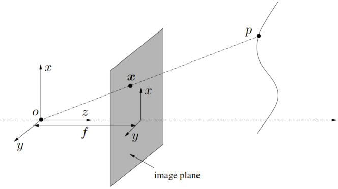
Figure 2.4: Perspective projection: $x$ is a point on the image plane, $p$ is its pre-image, a point in space. Vice-versa, if $p$ is a point in space, $x$ are the coordinates of its image, under perspective projection.

This equation is not satisfied for all $x\in D$, but only for those that are projection of points on the object, $x\in D\cap\pi(gS)$. Also, not all points $p\in S$ are visible, but only those that intersect the projection ray closest to the optical center. If we call $p_{1}$ the intersection of $S$ with the projection ray through the origin of the camera reference frame and the pixel with coordinates $x\in\mathbb{R}^{2}$, represented by the vector $\bar{x}$, we can write $p_{1}$ as the graph of a scalar function $Z:\mathbb{R}^{2}\rightarrow\mathbb{R}^{+};x\mapsto Z(x)$, the depth map. Here a bar $\bar{x}\in{\mathbb{P}}^{2}\simeq\mathbb{R}^{2}$ denotes the homogeneous (projective) coordinates of the point with Euclidean coordinates $x\in\mathbb{R}^{2}$: $\bar{x}=\left[\begin{array}[]{c}x\\ 1\end{array}\right]$. More in general, the pre-image of the point $x$ (on the image plane) is a collection of points (in space) given by

$$\pi^{-1}_{S}(x)=\{p_{1},\dots,p_{N}\in S\}=\{g^{-1}\bar{x}Z_{i}(x)\}_{i=1}^{N(x)}.$$ (2.7)

Note that the number of points in the pre-image depends on $x$, and is indicated by $N(x)$. The pixel locations where two pre-images coincide are the occluding boundaries, also known as silhouettes. For instance, $\{x\ |\ Z_{1}(x)=Z_{j}(x)\}$ for some $j=2,\dots,N$ is an occluding boundary. If we sort the points in order of increasing depth, so that $Z_{1}(x)\leq Z_{2}(x)\leq\dots\leq Z_{N}(x)$, then the pre-image, restricted to the point of first intersection, is indicated by

$$\pi^{-1}(x)=p_{1}=g^{-1}\bar{x}Z(x)$$ (2.8)

where we indicate $Z_{1}(x)$ simply with $Z(x)$. We omit the subscript $S$ in the pre-image for simplicity of notation, although we emphasize that it depends on the geometry of the surface $S$. We also omit the temporal index $t$, although we emphasize that, even when the scene $S$ is static (does not depend on time), changes of viewpoint $g_{t}$ will induce changes of the range map $Z_{t}(x)$. We also omit the contrast transformation $k$, that can also change over time, although we will re-consider all these choices later.

Note that the image only exists for $x\in D\cap\pi(gS)$, and the pre-image only exists for $p\in S\cap\pi^{-1}(D)$. For the region of the image where the scene is visible, say at time $t=0$, we can represent $S$ as the graph of a function defined on the domain of the image $I_{0}$, so $p=\pi^{-1}(x_{0})=\bar{x}_{0}Z(x_{0})$. Here $k$ can be taken to be the identity function, $k_{0}=Id$, so that $I_{0}(x_{0})=\rho(p)~{}~{}~{}p=\pi^{-1}(x_{0}).$ Therefore, combining this equation with (2.6), we have $I(x)=k\circ\rho\circ\pi^{-1}(x_{0})$, with the relation between $x$ and $x_{0}$ being

$$x=\pi gp=\pi g\pi^{-1}(x_{0})\doteq w(x_{0})$$ (2.9)

where $w:\mathbb{R}^{2}\rightarrow\mathbb{R}^{2}$ denotes the domain deformation induced by a change of viewpoint $g$, and the photometric relation being

$$I\circ w(x_{0})=k\circ I_{0}(x_{0}).$$ (2.10)

This is know as the “brightness constancy constraint equation.” Note that the two previous equations are simultaneously valid only in

$$x_{0}\in D\cap w(D)=D\cap\pi g\pi^{-1}(D)$$ (2.11)

which is called the co-visible region. It can be shown that the composition of maps $w:\mathbb{R}^{2}\rightarrow\mathbb{R}^{2};\ x_{0}\mapsto x=w(x_{0})\doteq\pi(g\bar{x}_{0}Z(x_{0}))$ spans the entire group of diffeomorphisms (Theorem 2 of [167]) as the function $Z(\cdot)$ is allowed to vary (which is necessary, unless it is known). In this model, visibility is captured by the map $\pi$ and its inverse. In particular, $\pi:\mathbb{R}^{3}\rightarrow\mathbb{R}^{2}$ maps any points in space $p$ into one location $x=\pi(p)$ on the image plane, assumed to be infinite. So the image of a point $p$ is unique. However, the pre-image of the image location $x$ is not unique, as there are infinitely many points that project onto it. If we assume that the world is populated by opaque objects, then the pre-image $\pi^{-1}_{S}(x)$ consists of all the points on the surface(s) $S$ that intersect the projection ray from the origin of the camera reference frame through the given image plane location $x$. This model does not include quantization, noise and other phenomena that are discussed in more detail in the appendix.

2.3 Marginalization, extremization (max-out), blurring

If we have prior knowledge on all the hidden variables, $\xi,g,\nu,n$, we can compute the likelihood in (2.4) by marginalization. This is conceptually trivial, but computationally prohibitive. Prior knowledge on the nuisance is encoded in a distribution $dP(\nu)$, which may have a density $p(\nu)$ with respect to a base measure $d\mu(\nu)$. Prior knowledge on the scene is encoded in the class-conditional distribution $dQ_{c}(\xi)$, which may again have a density $q(\xi|c)$ with respect to a base measure $d\mu(\xi)$. The same goes with the group $g$. We can reasonably assume that the residual, after all relevant aspects of the problem have been explicitly modeled, is a white zero-mean Gaussian noise $n\sim{\cal N}(0;\Sigma)$ with covariance $\Sigma$. Marginalization then consists of the computation of the following integral

$${p(I|c)=\int{\cal N}(I-h(g,\xi,\nu);\Sigma)dP(g)dP(\nu)dQ_{c}(\xi).}$$ (2.12)

The problem with this approach is not just that this integral is difficult to compute. Indeed, even for the simplest instantiation of the image formation model (2.6), it is not clear how to even define a base measure on the sets of scenes $\xi$ and nuisances $\nu$, let alone putting a probability on them, and learning a prior model. It would be tempting to discretize the model (2.6) to make everything finite-dimensional; unfortunately, because of scaling and quantization phenomena in image formation, any reasonable discretization of the scene would yield a very large scale inference problem. This integral is costly to compute even for the simplest characterizations of the scene and the nuisances. Indeed, the space of scenes (shape, radiance distribution functions) does not admit a “natural” or “sufficient” discretization. However, if one was able to do so, then a threshold on the likelihood ratio, depending on the priors of each class, yields the optimal (Bayes) classifier [150]. Recently, a local approximation of the above integral has been proposed in [51], and named R-HOG (reconstructive HOG).

An alternative to marginalization, where all possible values of the nuisance are considered with a weight proportional to their prior density, is to find the class together with the value of all the hidden variables that maximize the likelihood:

$${\tilde{p}(I|c)=\sup_{g,\nu,\xi}{\cal N}(I-h(g,\xi,\nu))p(g)p(\nu)q(\xi|c).}$$ (2.13)

This procedure of eliminating nuisances by solving an optimization problem is called “extremization” or sometimes “max-out” of the hidden variables. A threshold on the result yields the maximum likelihood (ML) classifier. Needless to say, this is also a complex procedure. This procedure also relates to registration or alignment between (test) data and a “template,” a common practice in pattern recognition. Recently, a local approximation of the above integral has been proposed in [51], and named MV-HOG (multi-view HOG).

A third alternative to obtain statistics that reduce the variability of the data with respect to nuisances is to average the data with respect to the group action. For instance, a function of the image that is invariant to planar rotations can be easily computed by averaging rotated versions of the image. This is clearly lossy, as there are many different scenes that produce the same invariant, so one may want to restrict the averaging to small transformations. If the averaging is done properly [31], the process can be made lossless and therefore provide true invariance, at least to a small group of transformations, but in general produces statistics that are insensitive (as opposed to “invariant” or “stable”). The next section describes an alternative, further elaborated in Section 3. Note that the max-out procedure can be understood as a special case of marginalization when the prior is uniform (possibly improper). Therefore, we will use the term marginalization to refer to either procedure, depending on whether or not a prior is available.

2.4 Features

A feature is any deterministic function of the data, $\phi:{\cal I}\rightarrow\mathbb{R}^{K};I\mapsto\phi(I)$, or sometimes $\phi\circ I$. In general, it maps onto a finite-dimensional vector space $\mathbb{R}^{K}$, although in some cases the feature could take values in an infinite-dimensional (function) space. Obviously, there are many kinds of features, so we are interested in those that are “useful” in some sense. The decision rule itself, $\hat{c}(I)$ is a feature. However, it does not just depend on the datum $I$, but also on the entire training set. Therefore, we reserve the nomenclature “feature” only for deterministic functions of the (sample) test data, but not on the training set. Deterministic functions of (ensemble) data are called “statistics.” We call any statistic of the training set (but not of the test datum) a template. For instance, the class-conditional mean is a template.

One can think of a feature as any kind of “pre-processing” of the data. The question as to whether such pre-processing is useful is addressed by the data processing inequality.

2.4.1 Data processing inequality

Let $R(I,c)$ be the conditional risk (2.1) associated with a decision $c$, and $\hat{c}:{\cal I}\rightarrow\{0,1\};I\mapsto\hat{c}(I)$ be the optimal classifier, defined as $\hat{c}=\arg\min_{c}R(I,c)$. Let $\phi:{\cal I}\rightarrow\mathbb{R}^{K}$ be any feature. Then, if $R(c)$ is the Bayes risk (2.3) associated with the classifier $c$, we have that

$$\min_{c}R(c)\leq\min_{\tilde{c}}R(\tilde{c}\circ\phi).$$ (2.14)

In other words, there is no benefit in pre-processing the data. This results follows simply from the Markov chain dependency $c\rightarrow I\rightarrow\phi$, known as “data processing inequality” ([42] Theorem 2.8.1, page 32, and the following corollary on page 33). Thus, it seems that the best one can do is to forgo pre-processing and just use the raw data. Even if the purpose of a feature $\phi(I)$ is to reduce the complexity of the problem, this is in general done at a loss, because one could include a complexity measure in the risk functional $R$, and still be bound by (2.14). However, there are some statistics that are “useful” in a sense that we now discuss.

2.4.2 Sufficient statistics

Those statistics that maintain the “=” sign in the data processing inequality (2.14) are called sufficient statistics for the purpose of this manuscript. Thus, $\phi:{\cal I}\rightarrow\mathbb{R}^{K}$ is a sufficient statistic if $\min_{c}R(c)=\min_{\tilde{c}}R(\tilde{c}\circ\phi)$. Of course, what is a sufficient statistic depends on the task, encoded in the risk functional $R$. A trivial sufficient statistic is the identity functional $\phi(I)=I$. Of all sufficient statistics, we are interested in the “smallest,” i.e. , the one that is a function of all other sufficient statistics. This is called the minimal sufficient statistic, which we indicate with $\phi^{\vee}(I)$.

Clearly, sufficiency and minimality represent useful properties of a statistic. A minimal sufficient statistic contains everything in the data that matters for the decision; no more (minimality) and no less (sufficiency). Unfortunately, (finite-dimensional) sufficient statistics do not always exist, so relaxed versions of the notion of sufficient statistics have been developed [173], and will be discussed later in this manuscript. Another useful property of a feature is that it contains nothing that depends on the nuisances.

2.4.3 Invariance

In the image-formation model (2.5), we have isolated nuisances that have the structure of a group $g$, those that are not, $\nu$, and then the additive “noise” $n$. The latter is a very complex process that has a very simple statistical description (e.g. independent and identically distributed samples from a Gaussian process in space and time). Instead, we focus on the group nuisances, $g\in G$ and on the non-invertible nuisances $\nu$. A statistic is $G$-invariant if it does not depend on the nuisance: $\phi(I)=\phi\circ h(g,\xi,\nu)=\phi\circ h(\tilde{g},\xi,\nu)$ for any two nuisances $g,\tilde{g}$ and for any $\nu$ and $\xi\in\Xi$ . One could similarly define an invariant feature for the non-invertible nuisances.

Any constant function is an invariant feature, $\phi(I)={\rm const},\ \forall\ I$; obviously it is not very useful. Of all invariant features, we are interested in the “largest,” in the sense that all other invariants are functions of it. We call this the maximal invariant, and indicate it with the symbol $\phi_{G}^{\wedge}(I)$ or $\phi^{\wedge}(I)$ when the group $G$ is clear from the context.

In general, there is no guarantee that an invariant feature, even the maximal one, be a sufficient statistic. In the process of removing the effects of the nuisances from the data, one may lose discriminative power, quantified by an increase in the expected risk. Vice-versa, there is no guarantee that a sufficient statistic, even the minimal, be invariant. In the best of all worlds, one could have a minimal sufficient statistic that is also invariant, or vice-versa that a maximal invariant that is sufficient. In this case, the feature $\phi^{\vee}(I)=\phi^{\wedge}(I)$ would be the best form of pre-processing one could hope for: It contains all and only the “information” the data contains about $\xi$, and have no dependency on the nuisance. We call a minimal sufficient invariant statistic a complete feature. Note that, in general, a complete feature is still not equivalent to $\xi$ itself, for the map $\xi\rightarrow\phi$ may not be injective (one-to-one). However, it can be shown that when the nuisance has the structure of a group, one can define an invariant statistical model (Definition 7.1, page 268 of [150]) and design a classifier, called equi-variant, that achieves the minimum (Bayesian) risk (see Theorem 7.4, page 269 of [150]). This can be done even in the absence of a prior, assuming a uniform (“un-informative” and possibly improper) prior. For this reason, we will be focusing on the design of invariants to the group component of the nuisance, an refer to $G$-invariants as simply invariants.

Therefore, if all the nuisances had the structure of a group $G$, i.e. when $\nu=0$, the maximal invariant would also be a sufficient statistic, and this would be a very fortunate circumstance (Example 1). Unfortunately, in vision this does not usually happen, since the nuisance groups of interest act on the scene, rather than the image. Nevertheless, it may be possible to compute invariants if we are willing to act (Section 8).

2.4.4 Representation

Given a scene $\xi$, we call ${\cal L}(\xi)$ the set of all possible images that can be generated by that scene up to an uninformative residual:

$${\cal L}(\xi)\doteq\{I\simeq h(g,\xi,\nu),~{}~{}~{}g\in G,\nu\in{\cal V}\}.$$ (2.15)

We have omitted the additive noise term since, in general, it describes the compound effect of multiple factors that we do not model explicitly, and therefore it is only described in terms of its ensemble properties from which it can be easily sampled. The $\simeq$ sign above indicates that the scene image is determined up to the additive residual $n$, which is assumed to be spatially and temporally white, identically distributed with an isotropic density (homoscedastic). It is, by definition, uninformative.

Given an image $I$, in general there are infinitely many scenes $\hat{\xi}$ that could have generated it under some unknown nuisances, so that

$$I\in{\cal L}(\hat{\xi}).$$ (2.16)

We call any such scene a representation compatible with that image. A representation is a feature, i.e. , a function of the data: It is the pre-image (under $\cal L$) of the measured image $I$: $\hat{\xi}\in{\cal L}^{-1}(I)$, and takes values in the space of all possible scenes $\Xi$.

A trivial example of a representation is the image itself glued onto a planar surface, that is $\hat{\xi}=(S,\rho)$ with $S=D\subset\mathbb{R}^{2}$ and $\rho=I$. Depending on how we define the nuisance $\nu$ in relation to the additive noise $n$, the “true” scene may not actually be a viable representation, which has subtle philosophical implications.

Note that there is no requirement that the representation $\hat{\xi}$ be unique, or have anything to do with the “true” scene $\xi$; the relation between the two is explored in Chapter 8.

While this concept of representation is pointless for a single image, it is important when considering multiple images of the same scene. In this case, the requirement is that the single representation $\hat{\xi}$ simultaneously “explains” an entire set of images $\{I\}$ of the same scene:

$$\hat{\xi}\in{\cal L}^{-1}(\{I\})\in\Xi.$$ (2.17)

Of all representations, we will be interested in either the “most probable,” if we are lucky enough to have a prior on the set of scenes $dQ(\xi)$, which is rare, or in the simplest one, which we call the minimal representation (a minimal sufficient statistic), and indicate with ${\hat{\xi}}^{\vee}$.

Given a scene $\xi$, we are particularly interested in the minimal representation that can generate all possible images that the original scene $\xi$ can generate, up to uninformative residuals. We call this a complete representation:

$${\hat{\xi}}{\rm\ is\ complete\ iff\ }{\cal L}(\hat{\xi})={\cal L}(\xi).$$ (2.18)

When clear from the context, we will omit the superscript ^∨, and refer to a minimal complete representation as simply the representation. The symbol ${\cal L}$ for the set of images that are generated by a representation is chosen because, as we will see, a complete representation is related to the light field of the underlying scene. Indeed, with any representation $\hat{\xi}$ one could synthesize, or hallucinate, infinitely many images via the image-formation model (2.5)

$$\hat{I}\simeq h(g,\hat{\xi},\nu),~{}~{}~{}\forall\ g,\nu.$$ (2.19)

In other words, a representation is a scene from which the given data can be hallucinated. We will elaborate the issue of hallucination in Section 3.1, where we will describe the relation to the light field. For the purpose of a visual decision task, a complete representation is as close as we can get to reality (the scene $\xi$) starting from the data.

2.5 Actionable Information and Complete Information

The complexity of the data, measured in various ways, e.g. via coding length or algorithmic complexity [108], has traditionally been called “information” in the context of data compression and transmission. Although the complexity of an image may be relevant to transmission and storage tasks (the most costly signal to transmit and store is white noise), it is in general not relevant to decision or control tasks. Extremely complex data, where all the complexity arises from nuisance factors, is useless for visual decisions, so one could say that such data is “uninformative.” Vice-versa, there could be very simple data that are directly relevant to the decision. So, the complexity of the data itself is not a viable measure of the information content in the data for the purpose of visual decisions. A natural image is not just a random collection of pixels; rather, an image is a sample from a distribution of (natural) images, $p(I)$, not a distribution in itself. So, if we want to measure the “informative content” of an image, we have to do so relative to the scene.

Setting aside technicalities that arise when the distributions are over continuous infinite-dimensional spaces, we define entropy formally as $H(I)\doteq E[\log p(I)]$ where the expectation is with respect to $p$ itself; that is, $H(I)=\int\log p(I)dP(I)$ (see [42] for details). Entropy measures the “uncertainty” or “information” about the random variable $I$. Other measures of complexity, such as coding length [42] or algorithmic complexity [100, 108], can be also related to entropy. The mutual information ${\mathbb{I}}(I;\xi)$ [42] between the image and the scene is given by $H(\xi)-H(\xi|I)$. It is the residual uncertainty on the scene $\xi$ when the image $I$ is given. This would be a viable measure of the information content of the image, if one were able to calculate it. As we have seen in the previous section, the “true” scene $\xi$ is an elusive concept. It certainly cannot be easily discretized or endowed with a base measure. In a sense, this manuscript explores ways to compute such a mutual information.

In particular, using the properties of mutual information, we have that ${\mathbb{I}}(\xi;I)=H(I)-H(I|\xi)$, and the latter denotes the uncertainty of the image given a description of the scene. This only depends on the sensor noise and other unmodeled phenomena, for all other nuisances are encoded in $\xi$, so it is not indicative of the informative content of the image. On the other hand, if most of the uncertainty in the image $I$ is due to nuisance factors, the quantity $H(I)$ is also not indicative of the informative content of the image. So, instead of $H(I)$, what we want to measure is $H(\phi^{\wedge}(I))$, that discounts the effects of the nuisances. This is called actionable information [162] and formalizes the notion of information proposed by Gibson [65]:

$$\boxed{{\cal H}(I)\doteq H(\phi^{\wedge}(I)).}$$ (2.20)

In Section LABEL:sect-control-recognition we will explore the relation between Actionable Information and the conditional entropy of the image given an estimated description of the scene. Now, it is possible that the maximal invariant of the data $\phi^{\wedge}(I)$ contains no information at all about the object of inference. What would be most useful to perform the task would be a complete representation, $\hat{\xi}$. Of all statistics of the complete representation we are interested in the smallest, so we could measure the complete information as the entropy of a minimal sufficient statistic of the complete representation.

$$\boxed{{\cal H}_{\xi}=H({\hat{\xi}})}$$ (2.21)

We will defer the issue of computing these quantities to Section 8, although one could already conjecture that

$${\cal H}(I)\leq{\cal H}_{\xi}.$$ (2.22)

It is important to notice that, whereas the scene $\xi$ consists of complex objects (shapes, reflectance functions) that live in infinite-dimensional spaces that do not admit simple base measures, let alone distributions of which we can easily compute the entropy, the representation $\hat{\xi}$ is a function of the measured data, which lives in a benign finite-dimensional space.

Example 1

It is interesting to notice that there are cases when ${\cal H}(I)={\cal H}_{\xi}$. This happens, for instance, when the only existing nuisances have the structure of a group. For instance, if contrast is the only nuisance, then the geometry of the level lines (or equivalently the gradient direction) is a complete contrast invariant. Likewise, for viewpoint and contrast nuisances, the ART [167] is a complete feature.

2.6 Optimality and the relation between features and the classifier

Eliminating nuisances via marginalization yields classification that is “optimal” by definition. Eliminating nuisances via the design of invariant features yields optimal classification only if the nuisances have the structure of a group, i.e. $\nu=0$. That is, there are no other nuisances other than the group $G$ and the latter admits a representation on the image. In this case, one can “pre-process” both the data and the training set to eliminate the effects of $G$, and design an equivalent statistical model (called an “invariant” model), and an equi-variant classifier. In Section 4 we will show constructive ways of designing invariant features, via the use of co-variant detectors and their corresponding invariant descriptors.

Optimality, as we have defined it in (2.2), does not impose restrictions on the set of classifiers, and the data processing inequality (2.14) stipulates that any pre-processing can at best keep the Bayesian risk constant, but not decrease it. In the presence of only invertible nuisances, $\nu=0$, it is sensible to compute the maximal invariant to eliminate group nuisances, but non-invertible nuisances can only be eliminated without a loss at decision time, via marginalization or extremization. This puts all the burden on the classifier, that at decision time has to compute a complex integral (2.12), or solve a complex optimization problem (2.13).

An alternative to this strategy is to constrain the choice of classifiers by limiting the processing to be performed at decision time. For instance, one could constrain the classifiers to nearest-neighbor rules, with respect to the distance between statistics computed on the test data (features) and statistics computed on the training data (templates). Two questions then arise naturally: What is the “best” template, if there is one? Of course, even choosing the best template, a feature-template nearest neighbor is not necessarily optimal. Therefore, the second question is: When is a template-based approach optimal? We address these questions next.

2.6.1 Templates and “blurring”

This section refers to a particular instantiation of visual decision problems, where the set of allowable classifiers is constrained to be on the form

$${\hat{c}=\arg\min_{c\in\{0,1\}}d_{\phi}(I,\hat{I}_{c})=\|\phi(I)-\phi(\hat{I}_{c})\|}$$ (2.23)

for some statistic $\phi$ and some choice of distance or norm in the space of images. Here $\hat{I}_{c}$ is a function of the likelihood $p(I|c)$ that can be pre-computed, and is called a template. If the likelihood is given in terms of samples (training set) $\{I_{k}\}_{k=1}^{K}\sim p(I|c)$, then the template can be any statistic of the (training) data. In particular, a distance can be defined by designing features $\phi$ that are invariant to the group component of the nuisance $g\in G$. In this case, the space $\phi({\cal I})={\cal I}/G$ is the quotient of the set of images modulo the group component of the nuisance, which is in general not a linear space even when both $\cal I$ and $G$ are linear. The distance above is a cordal distance, that does not respect the geometric structure of the quotient space ${\cal I}/G$. A better choice would be to define a geodesic distance, or a distance between equivalence classes, $d_{G}([\phi(I)],[\phi(\hat{I}_{c})])$. The structure of orbit spaces of scenes under the action of finite-dimensional groups is conceptually clear and will not be further discussed here (see Appendix A.1). Instead, we focus on the two critical questions: First, what is the “best” template $\hat{I}_{c}$, and how can it be computed from the training set? Second, are there situations or conditions under which this approach can yield the same performance of the Bayes or ML classifiers? (Section 3). In Section 6 we will show that one can build the equivalent of a template also for the test set, provided that a “sufficiently exciting” test sample is available.

The first thing to acknowledge is that the “best” template depends on the class of discriminants (or distance functions) one chooses. We will therefore answer the question for the simplest case of the squared Euclidean distance in the embedding (linear) space of images $\mathbb{R}^{N\times M}$. More in general, the distance and its corresponding optimal template have to be co-designed [106, 105]. In all cases, one can choose as optimal template the one that induces the smallest expected distance for each class. For the case of the Euclidean distance we have

$$\hat{I}_{c}=\arg\min_{I_{c}}E_{p(I|c)}[\|I-I_{c}\|^{2}]=\int_{\cal I}\|I-I_{c}\|^{2}dP(I|c)$$ (2.24)

that is solved by the conditional mean and approximated by the sample mean obtained from the training set

$$\hat{I}_{c}=\int_{\cal I}IdP(I|c)=\sum_{I_{k}\sim p(I|c)}I_{k}=\sum_{\begin{array}[]{c}g_{k}\sim dP(g)\\ \nu_{k}\sim dP(\nu)\\ \xi_{k}\sim dQ_{c}(\xi)\end{array}}h(g_{k},\xi_{k},\nu_{k}).$$ (2.25)

Note that the distribution of the training samples, that in the integral above acts as an importance distribution, has to be “sufficiently exciting” [16], in the sense that the training set must be a fair sample from $p(I|c)$. If this is not the case, for instance in the trivial instance when all the training samples are identical, then the optimal template cannot be constructed. Different instantiations of this notation (corresponding to different choices of groups $G$, scene representation $\Xi$, and nuisances $\nu$, often not explicit but latent in the algorithms) yield Geometric Blur [20], where the priors $dP(g)$ are not learned but sampled in a neighborhood of the identity, and DAISY [30, 175], where instead of the intensity the template is comprised of quantized gradient orientation histograms. More in general, many models of early vision architectures include filtering steps, that mimic the quotienting operation to generate the invariant $\phi^{\wedge}(I)$, followed by a pooling or averaging operation, akin to computing the template above [31]. Note also that the choice of norm, or more in general of classification rule, affects the form of the template. For instance, if instead of the $\ell^{2}$ norm we consider the $\ell^{1}$ norm, the resulting template is the median, rather than the mean, of the sample distribution. Other statistics are possible, including the (possibly multiple) modes, or the entire sample distribution [105].

Note that the relationship between a template-based nearest-neighbor classifier and a classifier based on the proper likelihood is not straightforward, even if the class consists of a singleton – which means that it could be captured by a single “template” if there were no nuisances. The marginalized likelihood is

$$\int\exp\left(-\|I-h(g,\xi,\nu)\|_{\Sigma}^{2}\right)dP(g)dP(\nu)$$ (2.26)

assuming a normal density for the additive residual $n$, with covariance $\Sigma$, where $\|\cdot\|_{\Sigma}$ is a Mahalanobis norm, $\|v\|^{2}_{\Sigma}\doteq v^{T}\Sigma^{-1}v$; the nearest-neighbor template-based classifier would instead try to maximize

$$\exp\left(-\|I-\underbrace{\int h(g,\xi,\nu)dP(g)dP(\nu)}\|^{2}\right).$$ (2.27)

The quantity bracketed is called the blurred template $\hat{I}_{c}$

$${\hat{I}_{c}\doteq\int h(g,\xi,\nu)dP(\nu)dP(g)}$$ (2.28)

which does not depend on the nuisance not because it has been marginalized or max-outed, but because it has been “blurred” or “smeared” all over the template. This strategy does not rest on sound decision-theoretic principles, and yet it is one of the most commonly used in a variety of classification domains, from nearest neighbor [20] to support vector machines (SVM) [36] to neural networks [161], to boosting [184].

It should be clear that blurring is a lossy process, as aggregating the training set into a single statistic decreases the discriminative power of the approach. One could attempt to minimize the loss, as done by Mallat and co-workers [31], who devise an iterative coding/blurring process that is lossless in the limit, for sufficiently concentrated nuisance distributions; the process is then truncated after two stages and not carried to the limit, so the loss remains.

Note that if instead of computing distance in the embedding space $\|I-\hat{I}\|_{\cal I}$ we compute the distance in the quotient, ${\cal I/G}$, we do not need to blur out the group in the template. In fact, the expectation of the quantity

$$\exp\left(-d_{G}(\phi(I),\phi(\hat{I}))\right)$$ (2.29)

is minimized by

$$\phi(\hat{I})\doteq\int\phi\circ h(\xi,\nu)dP(\nu).$$ (2.30)

Note that we have implicitly assumed that $\phi$ acts linearly on the space $\cal I$, lest we would have to consider ${\widehat{\phi(I)}}$, rather than $\phi(\hat{I})$. We discuss linear features in more detail in Section 4.2.

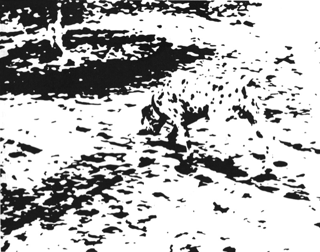
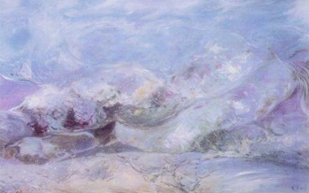
Figure 2.5: Complex nuisances (quantization, contrast, partial occlusions) can be so severe as to render a (single) template, $\hat{I}_{c}$ above, largely indiscriminative. Marginalization may enable recognition, especially if guided by priors. In some cases, even that does not work. However, extremization of the nuisances given the class can still be performed from (2.13). For instance, given the class $c=$“dalmatian” (left) and $c=$“back of a nude” (right), one can easily determine viewpoint (pose) $\hat{g}$, and occlusions (location) $\hat{\nu}$ from (2.13).

As for how the priors can be learned from the data, we defer the answer to Section 9 since it is not specific to the use of templates. For now, we note that – should a prior be available – it can be used according to (2.25) for the case of classifiers based on features/templates, (2.12) for the case of Bayesian and (2.13) for the case of ML classifiers.

The second question, which is under what conditions this template-based approach is optimal, is somewhat more delicate and will be addressed in Section 3.4. The short answer is never, in the sense that if it were optimal, there would be no need for averaging. However, a template approach can be advocated when there are constraint on decision-time, and at least some of the nuisances can be eliminated via canonization, as described in Section 3, and the residual uncertainty is described by a uni-modal class-conditional density that is well captured by its mode or mean (2.30).

When the template is computed on the test data, it can be used as a “descriptor”, that is, an invariant feature. More general descriptors will be discussed in the next chapter, and how to construct them from data will be described in Section 6.

Remark 1 (On the use of the word “template”)

The term template refers to a large variety of approaches, only some of which are captured by the definition we have given in this chapter. In particular, Deformable Templates, studied in depth by Grenander and coworkers [70], are based on premises that are not valid in our setting. In fact, in Deformable Templates there is an underlying hidden variable, the “template” (which could be given or learned), that is acted upon by a “deformation” (typically an infinite-dimensional group of diffeomorphisms). However, in Grenander’s approach the group acts transitively on the template, meaning that from the template one can “reach” any object of interest. In other words, there is a single orbit that covers the entire space of the measurements. In this case, all the “information” is contained in the deformation (the group), that is therefore not a nuisance.

To introduce the next chapter, we consider the simple example of classification of hand-written digits. This is simple because the data formation process lacks the two fundamental phenomena we discussed in the previous chapter: Scaling and occlusion. The only nuisance variability is due to small deformations of the domain (geometric deformations, including misalignment), and range (stroke thickness). Fig. 2.6 shows a collection of images from the MNIST Digit dataset and the corresponding blurred templates. Then further templates are shown when the dataset is blurred with respect to additional translation, Euclidean transformations, and affine transformations. It is clear that discriminative power has been lost, since the digits can hardly be recognized from the blurred template. However, classification is increasingly insensitive to the transformations being considered, as the distance to a template changes little as the test sample is, respectively, translated, translated and rotated, or transformed with an affine map.

The likelihood of a test sample under the blurred template changes depending on whether the template has been blurred, or whether the nuisance transformation has been marginalied, or eliminated with max-out. The latter two operations entail an integral or a search at test time. When the nuisance is canonized, through a process that we describe in the next chapter, test-time complexity is the same as when the template is blurred, but the likelihood is similar to the case when the nuisance is marginazlied or max-outed.

Figure 2.6: Samples from the MNIST dataset of hand-written digits that have been aligned with respect to small affine transformations [188]. The resulting templates still exhibit some discriminative power, as the digits are discernible from the templates. If, however, nuisance transformations are included in the computation of the blurred template, the discriminative power reduces significantly, as the digits are barely discernible from the template. On the flip-side, the comparison is insensitive to misalignment of the test digit. Marginalizing or max-outing the nuisance transformations retains the discriminative power, but at an expense in run-time complexity. Canonizing the nuisance transformations achieves the best compromise of retaining discriminative power, achieving invariance to nuisance transformations, and minimizing run-time complexity.

Chapter 3 Canonized Features

Invariant features can be designed in a number of ways. In this section we describe a constructive approach called canonization, that leverages on the notion of co-variant detector and its associated invariant descriptor. This is also related to the notions of alignment and registration. The basic idea is that a group $G$ acting on a space $\Xi$ organizes it into orbits, $[\xi]\doteq\{g\xi\ \forall\ g\in G\}$ each orbit being an equivalence class (reflexive, symmetric, transitive) representable with any one element along the orbit. Of all possible choices of representatives, we are looking for one that is canonical, in the sense that it is isolated and can be determined consistently for each orbit. This corresponds to cutting a section (or base) of the orbit space. All considerations (defining a base measure, distributions, discriminant functions) can be restricted to the base, which is now independent of the group $G$ and effectively represents the quotient space ${\cal I}/G$. Alternatively, one can use the entire orbit $[\xi]$ as an invariant representation, and then define distances and discriminant functions among orbits, for instance via max-out, $d([\xi_{1}],[\xi_{2}])=\min_{g_{1},g_{2}\in G}d(g_{1}\xi_{1},g_{2}\xi_{2})$, as we discussed in the previous chapter.

The name of the game in canonization is to design a functional – called feature detector – that chooses a canonical representative for a certain nuisance $g$ that is insensitive to (ideally independent of) other nuisances. We will discuss the issue of interaction of nuisances in canonization in Section 3.4. Before doing so, however, we recall some nomenclature.

Definition 1 (Invariant Feature)

A feature $\phi:{\cal I}\rightarrow\mathbb{R}^{K}$ is any deterministic function of the data taking values in some vector space, $I\mapsto\phi(I)$. Considering the formal generative model (2.5), a feature is $G$-invariant if

$$\phi\circ h(g,\xi,\nu)=\phi\circ h(e,\xi,\nu),~{}~{}~{}\forall\ g\in G$$ (3.1)

and for all $\xi,\nu$ in the appropriate spaces, where $e\in G$ is the identity transformation.

In other words, an invariant feature is a function of the data that does not depend on the nuisance. Note that we are focusing on the group component of the nuisance, for reasons explained in the previous chapter and further elaborated in Section 3.4. We recall the definition of representation from Section 2.4.4:

Definition 2 (Representation)

Given a collection of images $\{I\}$, a feature $\hat{\xi}\in\Xi$ is a representation if $\{I\}\in{\cal L}(\hat{\xi})$, where ${\cal L}(\hat{\xi})=\{h(g,\hat{\xi},\nu),~{}~{}g\in G,\nu\in{\cal V}\}$. Equivalently, $\hat{\xi}\in{\cal L}^{-1}(\{I\})$. Given a scene $\xi$, a representation $\hat{\xi}$ is complete if it satisfies the compatibility condition ${\cal L}(\hat{\xi})={\cal L}(\xi)$; a minimal complete representation is a minimal sufficient statistic of ${\cal L}(\xi)$.

A representation is three things at once: It is a statistic, that is a function of the images. However, it is embedded in the space of scenes, so it can be thought of as a scene itself. For instance, given a single image, under the Lambert-Ambient-Static model (2.6) of Section 2.2, one can construct a representation that is a plane (shape $S$) with the image $I$ glued onto it, so $\rho=I$. Finally, the representation is a finite-complexity data structure that can be stored in the memory of a digital computer. We call it a “feature,” even though it lives in the embedding space of the scene, because, as we will show in Section 8, it can be computed from data.

A minimal complete representation, which we refer to as a “representation” without additional qualifications when clear from the context, would be the ideal feature, in the sense that it captures everything about the scene that can be gathered from the data except for the effect of the nuisances. When non-invertible nuisances are absent, $\nu=0$, a representation can be used as a representative of the orbits (equivalence classes) $[\xi]$:

$$\hat{\xi}=\phi^{\wedge}(h(g,\xi,0))\sim h(e,\xi,0).$$ (3.2)

Clearly the absence of non-invertible nuisances is a rare phenomenon, especially in vision where scaling and occlusion phenomena are dominant. Nevertheless, there are some cases of practical relevance where non-invertible nuisances are by and large absent (other than the additive “noise” component), such as the classification of hand-written digits of Fig. 2.6. The case where other nuisances are present, $\nu\neq 0$, requires some attention and will not be fully addressed until after Section 3.4. In the next section, however, we pause to elaborate on the notion of representation and what it entails. Then, we study the groups $G$ for which complete features exist (Section 3.4).

3.1 Hallucination and representation

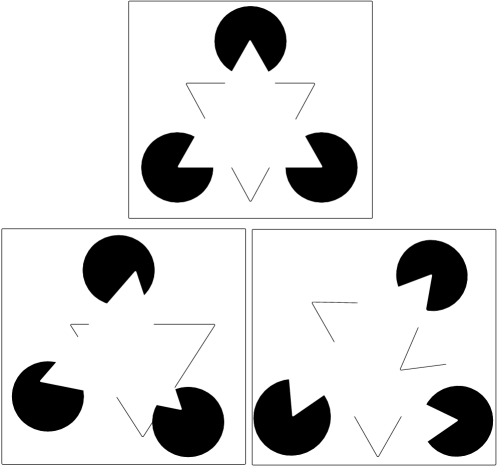
Figure 3.1: A representation enables the synthesis of an arbitrary number of images, and an image is compatible with infinitely many representations. Kanisza’s triangle (top) is an image that is compatible with multiple representations (e.g. the two scenes on the bottom). There is no way, from an image alone or without further exploration, to ascertain which representation is “correct.” A unique interpretation can be forced by imposing priors or other model selection criteria (e.g. minimum description), but the process is problematic from an epistemological stance. On the other hand, if one is allowed to gather more data, for instance as part of an exploration process as described in Section 8, the set of representations that is compatible with the data shrinks. For instance, of all the representations compatible with the top image, only a subset will also be compatible with the bottom-right, and another subset with be compatible with the bottom-left. While it is not possible to say, even asymptotically with an infinite amount of data, whether the representation approaches in some sense the “true” scene, it is possible to validate whether the representation is compatible with the true scene in the sense of ${\cal L}(\hat{\xi})={\cal L}(\xi)$. In the case above, given the top image and one of the bottom two, it is possible to determine whether the representation is compatible with two triangles and three discs or three pac-man figures and three wedges.

If there were only invertible nuisances, there would be no need for a notion of representation, since the equivalence class $[h(g,\xi,0)]$ is a complete feature and it can be inferred from a single datum. One would only have to learn the intra-class variability, that some have argued is considerably simpler [143]. To begin understanding the notion of representation in the presence of non-invertible nuisances, we need to go back to the image formation model (2.6), and in particular to the pre-image of a point $x\in D$ on the domain of an image (2.7):

$$\pi^{-1}_{S}(x)=\{p\in S\ |\ \pi(p)=x\}.$$ (3.3)

We note that this set may contain multiple elements, and in particular all points that lie on the same projection ray $\bar{x}$:

$$\pi^{-1}_{S}(x)=\{\bar{x}Z_{i}(x)\in S\}_{i=1}^{N(x)}.$$ (3.4)

We recall from (2.7) that we sort the depths $Z_{i}$ in increasing order, $Z_{1}(x)\leq Z_{2}(x)\leq\dots\leq Z_{N}(x)$, and when we want to restrict the pre-image to the point of first intersection, $Z(x)=Z_{1}(x)$, we indicate the (unique) pre-image via $\pi^{-1}(x)=\bar{x}Z(x)$ where $Z(x)=Z_{1}(x)$ (i.e. , we forgo the subscript $S$, even though the pre-image of course does depend on the shape of the scene $S$). Note that both $\pi^{-1}(x)$ and $\pi^{-1}_{S}(x)$ depend on the viewpoint $g$ and on the geometry and topology of the scene. They depend on how many simply connected components $S_{i}$ there are (“detached objects”), how many holes, openings, folds, occlusions etc. Note that we have sorted the depths while allowing the possibility of multiple points at the same depth. This happens in the limit when $x$ approaches an occluding boundary.

Remark 2 (The “ideal image”)

In Section 2.4.4 we have hinted at the fact that the scene itself may not be a viable representation of the images that it has generated, which may appear strange at first. Indeed, the “true” scene may never be known, because it exists at a level of granularity that is finer than any instrument we have available to measure it. So, we only have access to the “true” scene via the data formation process (visual or otherwise). This is unlike a representation $\hat{\xi}$, that can be arbitrarily manipulated in order to generate any image $\hat{I}\in{\cal L}(\hat{\xi})$.

In the presence of occlusions, evaluating the (hypothetical) “ideal image” $h(e,\xi,0)$, that is the image that would be obtained if there were no nuisances, requires the “inversion” of the occlusion process, including a description of the scene both in the visible and in the non-visible portions. In formulas, from (2.6) and (2.7), we have

$$\boxed{h(e,\xi,0)=\rho\left(\pi^{-1}_{S}(D)\right).}$$ (3.5)

Note that what this object returns is not the shape $S$ of the scene, but the radiance of the scene in both the visible and the occluded portions of the scene. So, in a sense, it is an image of a “semi-transparent world” made of many simply connected surfaces. Note, however, that the 3-D geometry may be recovered if we can control the data acquisition process via $h(g,\xi,0)$, with $g=g(u)$ as described in Chapter 8, because by doing so we can generate the collection of all possible occluding boundaries, which is equivalent to an approximation of the 3-D geometry of the scene [199]. In any case, the hypothetical image $h(e,\xi,0)$ captures the topology of the world, reflected in the number of layers $N$ present in the pre-image. While the notion of ideal image is awkward, and we will soon move beyond it, we need to consider it for a little while longer to ascertain what would be possible (or may be possible, depending on the sensing modality) if there were only invertible nuisances.

As we have anticipated in Section 2.4.4, building a representation from a single image would not be very useful, because in general the space of all scenes $\Xi$ is much larger than the space of all images $\cal I$, and lifting the image onto the scene yields no practical benefit. However, one may be able to construct a representation $\hat{\xi}$ that is compatible with a collection of images, $\{I_{k}\}_{k=1}^{K}$, in the sense that

$$I_{k}=h(g_{k},\xi,\nu_{k})+n_{k}\simeq h(\hat{g}_{k},\hat{\xi},\hat{\nu}_{k})$$ (3.6)

for all $k=1,\dots,K$ and for some $\hat{g}_{k},\hat{\nu}_{k}$, but the same $\hat{\xi}$. In fact, once we have an hallucinated scene $\hat{\xi}$, we can produce infinitely many “virtual” images, that we can then compare with any real image that is actually measured. In fact, ${\cal L}(\hat{\xi})$ produces the set of all possible hallucinated images of the scene $\hat{\xi}$, and is therefore equivalent to its light field [99]. While the hypothesis $\hat{\xi}=\xi$ cannot be tested, and a meaningful distance $d(\xi,\hat{\xi})$ cannot be computed (we do not even have a metric in the space $\Xi$), the hypothesis $h(g,\xi,\nu)\simeq h(\hat{g},\hat{\xi},\hat{\nu})$ for some $\hat{g},\hat{\nu}$ can be very simply tested by comparing two images, which is a task that poses no philosophical or mathematical difficulties. In compact notation, what we can test is $\hat{\xi}\in{\cal L}^{-1}\left({\cal L}(\xi)\right)$. We will return to this issue in Sections 5.1 and 8.

So far we have described the hallucination process, by which a representation can be used to generate images. The inverse process of hallucination is exploration, by which one can use images to construct a representation. In Section 8 we will show how to perform this limit operation. Exactly how the representation $\hat{\xi}$, built through exploration, is related to the actual “real” scene $\xi$, for instance whether they are “close” in some sense, hinges on the characterization of visual ambiguities, which we discuss in Appendix B.3.

We will come back to the notion of representation after establishing what could be done if only invertible nuisances were present, and establishing exactly what nuisances are indeed invertible.

3.2 Optimal classification with canonization

In this section and the next we elaborate on what would be possible if all nuisances were invertible. So, we assume that $\nu=0$, and focus on the role of $g$. We will address $\nu\neq 0$ in Section 3.4. For now, we are interested in how to design invariant and sufficient statistics for $g$ alone, as if all other nuisances were absent. In this case, we can assume that the group $g$ acts on the space of images, or that the space of scenes and the space of images coincide.

One of the many possible ways of designing an invariant feature is to use the data $I$ to “fix” a particular group element $\hat{g}(I)$, and then “undo” it from the data. If the data does not allow fixing a group element $\hat{g}$, it means it is already invariant to $G$. So, we define a (co-variant) feature detector to be a functional designed to choose a particular group action $\hat{g}$, from which we can easily design an invariant feature, often referred to as an invariant (feature) descriptor. Note that both the detector and the descriptor are deterministic functions of the data, hence both are features. One can think of this process as some kind of registration, or alignment, but rather than registering to a target, it is a form of “self-alignment.”

We consider the set of digital images ${\cal I}$ to be functions $I:\mathbb{R}^{2}\rightarrow\mathbb{R}^{+};\ x\in{\cal B}_{\epsilon}(x_{ij})\mapsto I_{ij}$. Because of spatial quantization, they are piecewise constant and thus can be identified with the set of matrices $\mathbb{R}^{N\times M}$. A differentiable functional $\psi:{\cal I}\times G\rightarrow\mathbb{R};(I,g)\mapsto\psi(I,g)$ is said to be local, with effective support $\sigma$ if its value at $g$ only depends on a neighborhood of the image of size $\sigma>0$, up to a residual that is smaller than the mean quantization error. For instance, for a translational frame $g$, if we call $I_{|_{{\cal B}_{\sigma}(g)}}$ an image that is identical to $I$ in a neighborhood of size $\sigma$ centered at position $g\equiv T$, and zero otherwise, then $\psi(I_{|_{{\cal B}_{\sigma}(g)}},g)=\psi(I,g)+\tilde{n}$, with $|\tilde{n}|\leq\frac{1}{NM}\sum_{i,j}|n_{ij}|$ the spatial quantization error. For instance, a functional that evaluates the image at a pixel $g\equiv T=x\in{\cal B}_{\epsilon}(x_{ij})$, is local with effective support $\epsilon$. For groups other than translation, we consider the image in the reference frame determined by $g$, or equivalently consider the “transformed image” $I\circ g^{-1}$, in a neighborhood of the origin, so $\psi(I,g)=\psi(I\circ g^{-1},e)$.

If we call $\nabla\psi\doteq\frac{\partial\psi}{\partial g}$ the gradient of the functional $\psi$ with respect to (any) parametrization of the group, then under certain (so-called “transversality”) conditions on $\psi$, the equation $\nabla\psi=0$ locally determines $g$ as a function of $I$, $g=\hat{g}(I)$, via the Implicit Function Theorem. Such conditions are independent of the parametrization and consist of the Hessian matrix $H(\psi)\doteq\nabla\nabla\psi$ (i.e. the Jacobian of $\nabla\psi$) being non-singular, $\det(H(\psi))\neq 0$. The function $\hat{g}$ is unique in a neighborhood where the transversality condition is satisfied, and is called a (local) canonical representative of the group. If the canonical representative co-varies with the group, in the sense that $\hat{g}(I\circ g)=(\hat{g}\circ g)(I)$, then the functional $\psi$ is called a co-variant detector. Each co-variant detector determines a local reference frame so that, if the image is transformed by the action of the group, a hypothetical observer attached to the co-variant frame (i.e., a “Lagrangian” observer) would see no changes. We summarize this in the following definition:

Definition 3 (Co-variant detector)

A differentiable functional $\psi:{\cal I}\times G\rightarrow\mathbb{R};\ (I,g)\mapsto\psi(I,g)$ is a co-variant detector if

1. The equation $\det\left(H(\psi(I,g))\right)=0$ locally determines a unique isolated extremum in the frame $g\in G$, and

2. if $\nabla\psi(I,\hat{g})=0$, then $\nabla\psi(I\circ g,\hat{g}\circ g)=0\ \forall\ g\in G$, i.e. , $\psi$ co-varies with $G$.

The notation $I\circ g$ indicates the map $(I,g)=(h(e,\xi,0),g)\mapsto h(g,\xi,0)\doteq I\circ g$. This may seem a little confusing at this point, since the group is acting on the scene, but is being canonized by acting on the image. This will be clarified in Sect. 3.4.1. The first “transversality” condition [71] corresponds to the Jacobian of $\nabla\psi$ with respect to $g$ being non-singular:

$$|J_{\nabla\psi}|\neq 0.$$ (3.7)

In words, a co-variant detector is a function that determines an isolated group element in such a way that, if we transform the image, the group elements is transformed in the same manner. Examples of co-variant detectors will follow shortly.

Definition 4 (Canonizability)

We say that the image $I$ is $G$-canonizable (is canonizable with respect to the group $G$), and $\hat{g}\in G$ is the canonical element, if there exists a covariant detector $\psi$ such that $\nabla\psi(I,\hat{g})=0$.

Note that, depending on the functional $\psi$, the canonical element may be defined only locally, i.e. the functional may only depend on $I(x)_{|_{x\in{\cal B}\subset D}}$, that is a restriction of the image to a subset $\cal B$ of its domain $D$. In the latter case we say that $I$ is locally canonizable, or, with an abuse of nomenclature, we say that the region $\cal B$ is canonizable.

The transversality condition (3.7) guarantees that $\hat{g}$, the canonical element, is an isolated (Morse) critical point [128] of the derivative of the function $\psi$ via the Implicit Function Theorem [71]. So a co-variant detector is a statistic (a feature) that “extracts” a group element $\hat{g}$. With a co-variant detector we can easily construct an invariant descriptor, or local invariant feature, by considering the data itself in the reference frame determined by the detector:

Definition 5 (Canonized descriptor)

For a given co-variant detector $\psi$ that fixes a canonical element $\hat{g}$ via $\nabla\psi(I,\hat{g}(I))=0$ we call the statistic

$$\boxed{\phi(I)\doteq I\circ{\hat{g}}^{-1}(I)~{}~{}|~{}~{}\nabla\psi(I,\hat{g}(I))=0.}$$ (3.8)

an invariant descriptor.

Note that the descriptor is invariant with respect to the same group $G$ that is canonized by the detector. Obviously it is not invariant to other nuisances, including groups other than the one chosen to design the detector.

A trivial example of canonical detector and its corresponding descriptor can be designed for the translation group. Consider for instance the detector $\psi$ that finds the brightest pixel in the image. Relative to this point, that is, if we assign that point to the coordinate $(0,0)$, the image is translation-invariant. This is because, as the image translates, so does its brightest pixel, and in the moving frame the image does not change as we translate. Similarly, we can assign the value of the brightest pixel to $1$, the value of the darkest pixel to $0$, linearly interpolate pixel values in between, and we have an affine contrast-covariant detector and the associated contrast-invariant descriptor.

As far as eliminating the effects of a group, all covariant detectors are equivalent. Where they differ is in how they behave relative to all other nuisances. Later we will give more examples of detectors that are designed to “behave well” with respect to other nuisances. In the meantime, however, we state more precisely the fact that, as far as dealing with a group nuisance, all co-variant detectors do the job.

Theorem 1 (Canonized descriptors are complete features)

Let $\psi$ be a co-variant detector. Then the corresponding canonized descriptor (3.8) is an invariant sufficient statistic.

Proof: To show that the descriptor is invariant we must show that $\phi(I\circ g)=\phi(I)$. But $\phi(I\circ g)=(I\circ g)\circ{\hat{g}}^{-1}(I\circ g)=I\circ g\circ(\hat{g}g)^{-1}=I\circ g\circ g^{-1}{\hat{g}}^{-1}(I)=I\circ{\hat{g}}^{-1}(I).$ To show that it is complete it suffices to show that it spans the orbit space ${\cal I}/G$, which is evident from the definition $\phi(I)=I\circ g^{-1}$.
The notation $I\circ g$ is slightly ambiguous at this point, but will be clarified in Sect. 3.4.1.

Note that invertible nuisances $g$ may act on the domain of the image (e.g. affine transformations due to viewpoint changes), as well as on its range (e.g. contrast transformations due to illumination changes).

Example 2 (SIFT detector and its variants)

To construct a simple translation-covariant detector, consider an isotropic bi-variate Gaussian function
${\cal N}(x;\mu,\sigma^{2})=\frac{1}{{2\pi}\sigma}\exp(-\frac{\|x-\mu\|^{2}}{2\sigma^{2}})$; then for any given scale $\sigma$, the Laplacian-of-Gaussian (LoG) $\psi(I,g)\doteq\nabla^{2}{\cal N}(x;g,\sigma^{2})*I(x)$ is a linear translation-covariant detector. If the group includes both location and scale, so $\bar{g}=(g,\sigma^{2})$, then the same functional can be used as a translation-scale detector. Other examples are the difference-of-Gaussians (DoG) $\psi(I,g)\doteq\frac{{\cal N}(x;g,\sigma^{2})-{\cal N}(x;g,k^{2}\sigma^{2})}{k-1}*I(x)$, with typically $k=1.6$, and the Hessian-of-Gaussian (HoG) is $\psi(I,g)=\det H({\cal N}(x;g,\sigma^{2}))$. Among the most popular detectors, SIFT uses the DoG, as an approximation of the Laplacian.

Example 3 (Harris’ corner and its variants)

Harris’ corner and its variants (Stephens, Lucas-Kanade, etc.) replace the Hessian with the second-moment matrix:

$$\psi(I,g)\doteq\det\left(\int_{{\cal B}_{\sigma}(g)}\nabla^{T}I\nabla I(x)dx\right).$$ (3.9)

One can obtain generalizations to groups other than translation in a straightforward manner by replacing ${\cal N}(x;g,\sigma^{2})$ with $\frac{1}{{2\pi}\sigma\det J}\exp(-\frac{\|g^{-1}(x)\|^{2}}{2\sigma^{2}\det(J_{g})^{2}})$ where $J_{g}$ is the Jacobian of the group. For instance, for the affine group $g(x)=Ax+b$, we have that $\psi(I,g)=\nabla^{2}\left(\frac{1}{2\pi\sigma\det A}\exp(-\frac{\|A^{-1}(x-b)\|^{2}}{2\sigma^{2}\det(A)^{2}})\right)$ is an affine-covariant (Laplacian) detector. One can similarly obtain a Hessian detector or a DoG detector. The Euclidean group has $A\in SO(2)$, so that $\det{A}=1$, and the similarity group has $\tilde{\sigma}A$, with determinant $\tilde{\sigma}$.

As we will see in Example 6, this functional has some limitations in that it is not a linear functional, and therefore it does not commute with additive nuisances such as quantization or noise.

Example 4 (Harris-Affine)

The only difference from the standard Harris’ corner is that the region where the second-moment matrix is aggregated is not a spherical neighborhood of location $g$ with radius $\sigma$, but instead an ellipsoid represented by a location $T\in D\subset\mathbb{R}^{2}$ and an invertible $2\times 2$ matrix $A\in{GL}(2)$. In this case, $g=(T,A)$ is the affine group, and the second-moment matrix is computed by considering the gradient with respect to all $6$ parameters $T,A$, so the second-moment matrix is $6\times 6$. However, the general form of the functional is identical to (3.9), and shares the same limitations, as we will see, in that affine-covariant canonization necessarily entails a loss.

Although these detectors are not local, their effective support can be considered to be a spherical neighborhood of radius a multiple of the standard deviation $\sigma>0$, so they are commonly treated as local. Varying the scale parameter $\sigma$ produces a scale-space, whereby the locus of extrema of $\psi$ describes a graph in $\mathbb{R}^{3}$, via $(x,\sigma)\mapsto\hat{x}=\hat{g}(I;\sigma)$. Starting from the finest scale (smallest $\sigma$), one will have a large number of extrema; as $\sigma$ increases, extrema will merge or disappear. Although in two-dimensional scale space extrema can also appear as well as split, such genetic effects (births and bifurcations) have been shown to be increasingly rare as scale increases, so the locus of extrema as a function of scale is well approximated by a tree, which we call the co-variant detection tree [106].

Remark 3 (Canonizability, saliency and the “sketch”)

The notion of canonizability is related to the notion of “sketchability” defined in [72], although the latter is introduced without ties to a specific task, and motivated in [118]. In the case of this manuscript, the notion of canonizability arises naturally from visual classification tasks, in the sense of providing a vehicle to design an invariant descriptor. It also relates to the notion of “saliency” defined in [179, 82], although again the latter stems from resource limitations rather than from a direct tie to a visual classification task.

Remark 4 (Invariant descriptors without co-variant detectors)

The assumption of differentiability in a co-variant detector can be easily lifted; in Section 4.3 we will show how to construct co-variant detectors that are not differentiable. Indeed, canonization itself is not necessary to design invariant descriptors. We have already mentioned “blurring” as a way to reduce (if not eliminate) the dependency of a statistic on a group, although that does not yield a sufficient statistic. However, even for designing complete (i.e. invariant and sufficient) features, canonization is not necessary. For instance, the geometry of the level curves – or its dual, the gradient direction – is a complete contrast-invariant which does not require a contrast-detector. Indeed, even the first condition in the definition of a co-variant detector is not necessary in order to define an invariant descriptor: Assume that the image $I$ is such that for any functional $\psi$, the equation $\nabla\psi(I,g)=0$ does not uniquely determine $\hat{g}=\hat{g}(I)$. That means that $|J_{\nabla\psi}|=0$ for all $\psi$, and therefore all statistics are already (locally) invariant to $G$. More in general, where the structure of the image allows a “stable” and “repeatable” detection of a frame $\hat{g}$, this can be inverted and canonized $\phi(I)=I\circ{\hat{g}}^{-1}$. Where the image does not enable the detection of a frame $\hat{g}$, it means that the image itself is already invariant to $G$. These statements will be elaborated in Section 3.5 where we introduce the notion of texture.

Intuitively, if a covariant detector is “unstable”, i.e. , $|J_{\nabla\psi}|\simeq 0$, then any function $\phi(I)$ is “insensitive” to $g$, in the sense that, assuming $\psi\circ I$ to be smooth, we have $\phi(I)\simeq\phi(I\circ g)$. This means that what we cannot canonize does not matter towards the goal of designing invariant (insensitive) statistics; it is already invariant (insensitive). Of course, these statistics will not be localized. In particular, the definition of canonizability, and its requirement that $\hat{g}$ be an isolated critical point, would appear to exclude edges and ridges, and in general co-dimension one critical loci that are not Morse critical points. However, this is not the case, because the definition of critical point depends on the group $G$, which can include discrete groups (thus capturing the notion of “periodic structures,” or “regular texture”) and sub-groups of the ordinary translation group, for instance planar translation along a given direction, capturing the notion of “edge” or “ridge” in the orthogonal direction. We will come back to the notion of stability in Section 4.1.

Remark 5 (Dense descriptors)

We emphasize that detectors’ only purpose is to avoid marginalizing the invertible component of the group $G$. However, at best such detectors can yield no improvement over marginalizing the action of $G$, that is to use no detector at all (Section 2.4.1). Therefore, one should always marginalize or max-out the nuisances if this process is viable given resource constraints. This is a design choice that has been explored empirically. In visual category recognition, some researchers prefer to use features selected around “keypoints,” whereas others prefer to compute “dense descriptors” at each pixel, or at a regular sub-sampling of the pixel grid, and let the classifier sort out which are informative, at decision time.

Remark 6 (Preview: Aliasing and Proper Sampling)

Canonizability, as we have defined it, entails the computation of the Jacobian, which is a differential operation. However, images are discrete, merely a sampled version of the underlying signal (assuming that is piecewise differentiable), that is the radiance of the scene. In any case, the differentiable approximation, or the computation of the Jacobian, entails a choice of scale, depending on which any given “structure” (isolated extremum) may or may not exist: A differential operator such as the Jacobian could be invertible at a certain scale, and not invertible at a different scale at the same location. Because the “true” scale is unknown (and it could be argued that it does not exist), canonizability alone is not sufficient to determine whether a region can be meaningfully canonized. “Meaningful” in this context indicates that a structure detected in an image corresponds to some structure in the scene, and is not instead a sampling artifact (“aliasing”) due to the image formation process, for instance quantization and noise. Therefore, an additional condition must be satisfied for a region to be “meaningfully” canonized. This is the condition of Proper Sampling that we will introduce in Section 5.1.

3.3 Optimality of feature-based classification

The use of canonization to design invariant descriptors requires the image to support “reliable” (in the sense of Definition 3) co-variant detection. As we have discussed in Remark 4, the challenge in canonization is not when the co-variant detector is unreliable, for that implies the image is already “insensitive” to the action of $G$. Instead, the challenge is when the covariant detector reliably detects the wrong canonical element $\hat{g}$, for instance where there are multiple repeated structures that are locally indistinguishable, as is often the case in cluttered scenes. We will come back to this issue in Section 5.2.

The good news is that, when canonization works, it simplifies visual classification by eliminating the group nuisance without any loss of performance. This was already illustrated empirically in Fig. 2.6, and is formalized by the following theorem.

Theorem 2 (Invariant classification)

If a complete $G$-invariant descriptor $\hat{\xi}=\phi(I)$ can be constructed from the data $I$, it is possible to construct a classifier based on the class-conditional distribution $dP(\hat{\xi}|c)$ that attains the same minimum (Bayesian) risk as the original likelihood $p(I|c)$.

The proof follows from the definitions and Theorem 7.4 on page 269 of [150]. The classifier based on the complete invariant descriptor is called equi-variant.

Based on this result, one would surmise that it is always desirable to canonize group nuisances, whether or not they come with a prior $dP(g)$. An important caveat is that, so far in this section, we have assumed that the non-invertible nuisance is absent, i.e. $\nu=0$, or that, more generally, the canonization procedure for $g$ is independent of $\nu$, or “commutes” with $\nu$, in a sense that we will make precise in Definition. 6. This is true for some nuisances, but not for others, even if they have the structure of a group, as we will see in the next section. There we will show that many group nuisances indeed cannot be canonized. These include the affine and projective group (scale, skew, deformation) as well as more complex nuisances that have to be dealt with either by marginalization (2.12), or by extremization (2.13).

3.4 Interaction of nuisances in canonization: what is really canonizable?

The previous section described canonization of the group nuisance $g\in G$ in the absence of other nuisances $\nu=0$. Unfortunately, some nuisances are clearly not invertible (occlusions, quantization, additive noise), and therefore they cannot be canonized. What is worse, even group nuisances may lose their invertibility once composed with non-invertible nuisances.

In this section, we deal with the interaction between invertible and non-invertible nuisances, so we relax the condition $\nu=0$ and describe feature detectors that “commute” with $\nu$. We show that the only subgroup of $G$ that has this property is the isometric group of the plane. That is, planar rotations, translations and reflections. Other nuisances, groups or not, have to be dealt with by marginalization or extremization if one wishes to retain optimal performance. This includes the similarity group of rotations translations and scale, that is instead canonized in [114], and the affine group, that is instead canonized in [126].

In order to simplify the derivation, we introduce the following notation, in part already adopted earlier in the proof of Theorem 1. The notation will be fully clarified in Sect. 3.4.1. If $\hat{I}$ is the “ideal image” (without nuisances, see Remark 2), $\hat{I}=h(e,\xi,0)$, then

$$\hat{I}\circ g \doteq h(g,\xi,0)$$ (3.10)

$$\hat{I}\circ\nu \doteq h(e,\xi,\nu).$$ (3.11)

The operators $(\cdot\circ g)$ and $(\cdot\circ\nu)$ can also be composed, $\hat{I}\circ g\circ\nu=h(g,\xi,\nu)$ and applied to an arbitrary image; for instance, if $I=h(g,\xi,\nu)$, then for any other $\tilde{g},\tilde{\nu}$ we have

$$I\circ\tilde{g}\circ\tilde{\nu}=h(\tilde{g}g,\xi,\tilde{\nu}\oplus\nu)$$ (3.12)

where $\oplus$ is a suitable composition operator that depends on the space where the nuisance $\nu$ is defined. Note that, in general, the action of the group and the other nuisances do not commute: $I\circ g\circ\nu\neq I\circ\nu\circ g$. When this happens we say that the group commutes with the (non-group) nuisance:

Definition 6 (Commutative nuisance)

A group nuisance $g\in G$ commutes with a (non-group) nuisance $\nu$ if

$$I\circ g\circ\nu=I\circ\nu\circ g.$$ (3.13)

Note that commutativity does not coincide with invertibility: A nuisance can be invertible, and yet not commutative (e.g. the scaling group does not commute with quantization).

For a nuisance to be canonizable without a loss, (i.e. , eliminated via pre-processing, or via a complete invariant feature) it not only has to be a group, but it also has to commute with the other nuisances. In the following we show that the only nuisances that commute with quantization are the isometric group of the plane. While it is common, following the literature on scale selection, to canonize it, scale is not canonizable without a loss, so the selection of a single representative scale is not advisable. Instead, a description of a region of an image at all scales should be considered, since scale, in a quantized domain, is a semi-group, rather than a group.

Interaction of group nuisances with quantization

Note that, per Theorem 2, only for canonizable nuisances can we design an equi-variant classifier via a co-variant detector and invariant descriptor. All other nuisances should be handled via marginalization or extremization in order to retain optimality (minimum risk), or via a template if one is willing to sacrifice optimality in favor of speed at decision time.

Theorem 3 (What to canonize)

The only nuisance that commutes with quantization is the isometric group of the plane, that is the group of rotations, translations and reflections.

Proof: We want to characterize the group $g$ such that $I\circ g\circ\nu=I\circ\nu\circ g$ where $\nu$ is quantization. For a quantization scale $\sigma$, we have the measured intensity (irradiance) at a pixel $x_{i}$

$$I\circ\nu(x_{i})\doteq\int_{{\cal B}_{\sigma}(x_{i})}I(x)dx=\int\chi_{{\cal B}_{\sigma}(x_{i})}(x)I(x)dx=\int\chi_{{\cal B}_{\sigma}(0)}(x-x_{i})I(x)dx\\ \doteq\int{\cal G}(x-x_{i};\sigma)I(x)dx$$ (3.14)

where ${\cal B}_{\sigma}(x)$ is a ball of radius $\sigma$ centered at $x$, $\chi$ is a characteristic function that is written more generally as a kernel ${\cal G}(x;\sigma)$, for instance the Gaussian kernel ${\cal G}(x;\sigma)\doteq{\cal N}(x;0,\sigma^{2})$, allowing the possibility of more general quantization or sampling schemes, including soft binning based on a partition of unity of $D$ rather than simple functions $\chi$. Now, we have

$$(I\circ\nu)\circ g(x_{i})=\left(\int{\cal G}(x-x_{i};\sigma)I(x)dx\right)\circ g=\int{\cal G}(x-gx_{i};\sigma)I(x)dx$$ (3.15)

whereas, with a change of variable $x^{\prime}\doteq gx$, we have

$$(I\circ g)\circ\nu(x_{i})=\int{\cal G}(x-x_{i};\sigma)I(gx)dx=\int{\cal G}(g^{-1}(x^{\prime}-gx_{i});\sigma)I(x^{\prime})|J_{g}|dx^{\prime}$$ (3.16)

where $|J_{g}|$ is the determinant of the Jacobian of the group $G$ computed at $g$, so that the change of measure is $dx^{\prime}=|J_{g}|dx$. From this it can be seen that the group nuisance commutes with quantization if and only if

$$\begin{cases}{\cal G}={\cal G}\circ g\\ |J_{g}|=1.\end{cases}$$ (3.17)

That is, the quantization kernel has to be $G$-invariant, ${\cal G}(x;\sigma)={\cal G}(gx;\sigma)$, and the group $G$ has to be an isometry. The only isometry of the plane is the set of planar rotations and translations (the Special Euclidean group $SE(2)$) and reflections. The set of isometries of the plane is often indicated by $E(2)$.

Corollary 1 (Do not canonize scale (nor the affine group))

The affine group does not commute with quantization, and in particular the scaling and skew sub-groups. As immediate consequence, neither do the more general projective group and the group of general diffeomorphisms of the plane. Therefore, scale should not be (globally) canonized and the scaling sub-group should instead be sampled. We will revisit this issue in Section 5.2 where we introduce the selection tree.

So, although [162] suggests that invariant sufficient statistics can be devised for general viewpoint changes, this is only theoretically valid in the limit when there is no quantization and the data is available at infinite resolution. In the presence of quantization, canonization of anything more than the isometric group is not advisable. Because the composition of scale and quantization is a semi-group, the entire semi-orbit – or a discretization of it – should be retained. This corresponds to a sampling of scales, rather than a scale selection procedure.

It should be noted that the sampling of the scale group could be performed uniformly, by selecting a number of equally spaced scales, or adaptively, depending on the signal. For instance, SIFT’s scale “selection” procedure [115], based on Lindeberg’s work [110], should be interpreted as an adaptive scale sampling, rather than a selection (canonization), since scale is not canonizable. Correctly, SIFT allows the selection of multiple scales at the same location, which are signal-dependent samples of scale at that location.

The additive residual $n(x)$ does not pose a significant problem in the context of quantization since it is assumed to be spatially stationary and white/zero-mean, so quantization actually reduces the noise level:

$$n(x_{i})=\int_{{\cal B}_{\sigma}(x_{i})}n(x)dx\stackrel{{\scriptstyle\sigma}}{{\longrightarrow}}0.$$ (3.18)

Instead, the other important nuisance is occlusion.

Interaction of group nuisances with occlusion: Local invariant features

Planar rotations do not generate occlusions, so canonization of rotation is, at least to first approximation, unaffected by occlusion. Translation, however, is. In particular, if planar translations are due to parallax, consisting of a translation of the optical center in front of a scene that is not flat and fronto-parallel, there will be occlusions unless the scene is concave. Therefore, translation cannot be globally canonized either. This means that one should consider the set of all possible translations and defer the treatment of the nuisance to training or testing. This is indeed an approach that has recently taken hold in the recognition literature [44, 178].

However, owing to the statistics of natural images [130, 136], the response of any translation-co-variant detector will be neither a unique global extremum nor the entire lattice $\Lambda=D\cap{\mathbb{Z}}^{2}$, but instead a discrete set of (multiple, isolated) critical points $T_{i}\in\Lambda$. Therefore, one could hypothesize that each of them is a viable canonical representative, and then test the hypothesis at decision-time. This means that one should construct multiple descriptors for each canonical translation, at multiple scales, and then marginalize or eliminate occlusions by a max-out procedure at decision time, that now corresponds to a (combinatorial) search among all possible canonical locations in putatively corresponding images. This is just like the case of (multiple) scale selection in SIFT, that we interpreted as adaptive sampling of the scale group. One can think of the multiple selections of location and scales as adaptive sampling of the group, or multiple local canonization procedures.

In either case, the procedure provides multiple similarity frames, one per each canonical translation $T_{i}$, and at that translation for each sample scale $\sigma_{j}$, and a canonized rotation $R_{ij}$:

$$\hat{g}_{ij}\doteq\{T_{i},\sigma_{j},R_{ij},m_{ij}\}$$ (3.19)

where we have indicated with $m_{ij}$ a canonized contrast transformation, although contrast can equivalently be eliminated by considering the level lines or the gradient direction as described in Section 6.1.

The image, or a contrast-invariant, relative to the reference frame identified by $\hat{g}_{ij}$ is then, by construction, invariant modulo a selection process, in the sense that the corresponding frame may or may not be present in another datum (e.g. a test image) depending on whether it is co-visible. Thus, we have a collection of local invariant features of the form

$$\phi_{ij}(I) = I\circ{\hat{g}}^{-1}_{ij}=I(R_{ij}^{T}(S_{j}^{-1}x-T_{i})),~{}~{}~{}$$ (3.20)

$$i,j=1,\dots N_{T},N_{S}|{\cal B}_{\sigma_{j}}(x+T_{i})\cap\Omega=\emptyset$$

where $S:\mathbb{R}^{2}\rightarrow\mathbb{R}^{2};\ x\mapsto S(x)=\sigma x$, with $\sigma>0$ is a scale transformation, with $S^{-1}(x)=x/\sigma$, $T\in\mathbb{R}^{2}$ is a planar translation, and $R\in SO(2)$ is a planar rotation [117]. Here $N_{T}$ and $N_{S}$ are the number of canonical locations and sample scales respectively. Note that the selection of occluded regions, which is excluded from the descriptor, is not known a-priori and will have to be determined at decision time as part of the matching process. In particular, given one image (e.g. the training image) $I_{1}$ and its features $\phi_{ij}(I_{1})$, and another image (e.g. the test image) $I_{2}$, and its features $\phi_{lm}(I_{2})$, marginalizing the nuisance amounts to testing whether $\phi_{ij}(I_{1})\simeq\phi_{lm}(I_{2})$, for all possible combinations of $i,j,l,m$, corresponding to the hypothesis that the canonical region around the canonical translation $T_{i}$ at scale $\sigma_{j}$ in image $I_{1}$ is co-visible with the region around the canonical translation $T_{l}$ at scale $\sigma_{m}$ in image $I_{2}$.

In this sense, we say that translation is locally canonizable: The description of an image around each $t_{i}$ at each scale $\sigma_{j}$ can be made invariant to translation, unless the region of size $\sigma_{j}$ around $t_{i}$ intersects the occlusion domain $\Omega\subset D$, which is a binary choice that can only be made at decision time, not by pre-processing test images independently.

This is particularly natural when translation is canonized using a partition of the image into $\epsilon$-constant statistics (“segments”), such as normalized intensity, color spectral ratios, or normalized gradient direction histograms. In fact, each region (a node in the adjacency graph) or each junction (a face in the adjacency graph) can be used to canonize translation, and the image can be described by the statistics of adjacent neighbors, as we illustrate in Section 4.3.

So, although translation is not globally canonizable, we will refer to its treatment as local canonization modulo a selection process to detect whether the region around the canonical representative is subject to occlusion. What we have in the end, for each image $I$, is a set of multiple descriptors (or templates), one per each canonical translation, and for each translation multiple scales, canonized with respect to rotation and contrast, but still dependent on deformations, complex illumination and occlusions. One can also think of local canonization as a form of adaptive sampling, where regions that are not covariant are excluded. The same reasoning can also be applied to scale, where one can think of (multiple) scale selection as adaptive sampling of scale.

In Section 4 we will show how to construct local co-variant detectors, and in Section 6 how to exploit this process to construct local invariant descriptors.

Remark 7 (When to avoid canonization)

Canonization is just a way to factor out simple nuisances. Because of occlusions, this canonization process reduces to feature selection (in each individual image) and combinatorial matching. This process represents an approximation of the “correct” marginalization or max-out procedure described in Section 2.3. Therefore, if computational resources allow, the best course of action is to max-out or marginalize the nuisance, i.e. to avoid the canonization process altogether. This choice is usually dictated by the application constraints, and should be made with knowledge of the tradeoffs involved: Canonization reduces the complexity of the classifier, but at a cost in discriminative power. Marginalization is the best option if one has a prior available. Otherwise, max-out is the best option if the classifier can be computed in time useful for the task at hand.

3.4.1 Clarifying the formal notation $I\circ g$

So far we have used the notation $I\circ g$ to indicate that, if $I=h(e,\xi,\nu)$, then $I\circ g=h(g,\xi,\nu)$. This may seem inconsistent, as the scene and the image live in different spaces, and therefore $g$ acting on $\xi$ is not the same as $g$ acting on $I$. We are now ready to explain this inconsistency.

For a nuisance $g$ to be eliminated in pre-processing without a loss, it has to be a group, as well as commute with non-group nuisances. After the discussion in the previous sections, this can be expressed as $h(g,\xi,\nu)=gh(e,\xi,\nu)$ for all $\nu$. Therefore, if we divide the group nuisance $g$ into an “invertible” component $g^{i}$ and a “non-invertible” component $g^{n}$, so that $I=h(g^{i}g^{n},\xi,\nu)$, we then have that

$$I=h(g^{i}g^{n},\xi,\nu)=g^{i}h(g^{n},\xi,\nu).$$ (3.21)

But because $g^{n}$ is not invertible, and therefore it cannot be eliminated in pre-processing without a loss, its group structure is of no use, and we might as well lump $g^{n}$ with the non-invertible nuisance $\nu$. Therefore, from this point on, we can assume as a formal model of image formation the following: $I_{t}=g_{t}h(e,\xi,\nu_{t})+n_{t}$, and for simplicity we can omit the identity $e$. Therefore, we can represent this equivalently a $I=gh(\xi,\nu)$ or $I=h(g,\xi,\nu)$. Now it should be clear that the (invertible) group $g$ can act on the image $I$, so the notation $I\circ g\doteq gI$ is justified.

For instance, in the Lambert-Ambient model, $I(x)=\rho(p)$, contrast normalization is commutative: A contrast transformation applied to the albedo $k(\rho(p))$ induces a contrast transformation on the image, and therefore it can be neutralized (“inverted”) by performing co-variant detection on the image. So, if $I(x)=k(\rho(p))$, then ${\hat{k}}^{-1}(I(x))={\hat{k}}^{-1}k(\rho(p))$, where $\hat{k}=\hat{k}(I)$, is invariant to contrast. Similarly, a planar rotation applied to the scene, $\rho(Rp)$, where

$$R=\left[\begin{array}[]{ccc}\cos\theta&-\sin\theta&0\\ \sin\theta&\cos\theta&0\\ 0&0&1\end{array}\right]$$

induces a rotation on the image plane, $I(rx)$ where

$$r=\left[\begin{array}[]{cc}\cos\theta&-\sin\theta\\ \sin\theta&\cos\theta\end{array}\right]$$

so $I(rx)=\rho(Rp)$. A choice of orientation on the image plane, corresponding to a canonical rotation $\hat{r}=\hat{r}(I)$ can then be used to canonize $R$. Calling

$$\hat{R}=\left[\begin{array}[]{cc}\hat{r}&\begin{array}[]{c}0\\ 0\end{array}\\ 0~{}~{}~{}0&1\end{array}\right]$$

we have that $I(\hat{r}^{-1}x)=I(\hat{r}^{T}x)=\rho(\hat{R}^{T}Rp)$ is invariant to a planar rotation $R$. The story is considerably different for translation, and for general rigid motions, including out-of-plane rotation.

A translation along the optical axis, $T=[0,\ 0,\ s]^{T}$ induces a transformation on the image plane that depends on the shape of the scene $S$. If the scene is planar and fronto-parallel, translation along the optical axis induces a re-scaling of the image plane, also a group: $I(sx)=\rho(p+T)$. However, if the scene is not planar and fronto-parallel, forward translation can generate very complex deformations of the image domain, including (self-) occlusions. Similarly, for translation along a direction parallel to the optical axis, $T=[u,\ v,\ 0]^{T}$, only if the scene is planar and fronto-parallel does this result in a planar translation, so that $I(x+[u,\ v]^{T})=\rho(p+T)$.

It should be mentioned that different data modalities yield different commutativity properties, so it is possible that for certain data types the entire group nuisances may be commutative. For instance, cast shadows are non-invertible nuisances in grayscale images. However, if one has multiple spectral bands available, then several contrast-invariant features, such as spectral ratios, can be employed to eliminate the cast shadows.

3.4.2 Local canonization of general rigid motion

As we have discussed, parallax motion, including translation and out-of-plane rotation, does not commute with rotation, therefore one can at best locally canonize it. If one wishes to eliminate the effects of an arbitrary rigid motion, the entire group of diffeomorphisms has to be canonized; as shown in [167], this comes at a loss of discriminative power, since scenes of different shape are lumped onto the same equivalence class. But since occlusions force locality, one can also approximate general diffeomorphisms locally, and therefore only canonize sub-groups of planar diffeomorphisms. There is then a tradeoff between the sub-group being canonized and the size of the domain where the canonization is valid. Given an arbitrary margin, there will be a domain where the deformation is approximated by a translation, a larger domain where it is approximated by an isometry, a larger domain yet where it is a similarity, an affine transformation, and a projective transformation.

To see that, consider a general rigid motion in space $(R,T)$. That induces a deformation of the image domain that can be described, in the co-visible regions, by equation (2.9). In more explicit form, if we represent shape $S$ as the graph of a function in one of the images, say at time $t=0$, so that $p=p(x_{0})=\bar{x}_{0}Z(x_{0})$, with $x_{0}\in D$, then under the assumptions of the Lambert-Ambient model, $I_{t}(x_{t})=\rho(p)=I_{0}(x_{0})$ where

$$x_{t}=w(x_{0})=\pi(R\bar{x}_{0}Z(x_{0})+T)=\frac{R_{(1:2,:)}\bar{x}_{0}Z(x_{0})+T_{(1:2)}}{R_{(3,:)}\bar{x}_{0}Z(x_{0})+T_{3}}$$ (3.22)

in the co-visible region $D\cap w(D)$. Here we have used Matlab notation, where $R_{(1:2,:)}$ means the first two rows of $R$.

Of course, the size of the region where the approximation is valid cannot be determined a-priori, and should instead be estimated as part of the correspondence hypothesis testing process [187]. However, it is common practice to select the size of the regions adaptively as a function of the scale of the translation-covariant detector. This will be further elaborated in Chapter 5.

In the next section we establish the relation between local canonization and texture.

3.5 Textures

This section establishes the link between the notion of canonization, described in the previous section, and the design of invariant features, tackled in the next section.

3.5.1 Defining “textures”

A “texture” is a region of an image that exhibits some kind of spatial regularity. Figure 3.2 shows some examples of what are often called regular textures. They share the spatial regularity of some elementary structure, or “texture element”, or “texton” [93]. The images in Figure 3.3, on the other hand, do not exhibit regular repetition of any such structure. Instead, they are characterized by the fact that some ensemble property of the image is spatially homogeneous, i.e. , some statistic is translation-invariant. Such ensemble properties are pooled in a region whose minimal size plays the role of the elementary texture element. Translation invariance of statistics is captured by the notion of stationarity [156]. For instance, a wide-sense stationary process has translation-invariant mean and correlation function. A strict-sense stationary process has translation-invariant statistics of all orders.

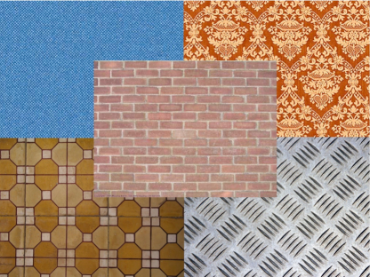
Figure 3.2: Regular textures

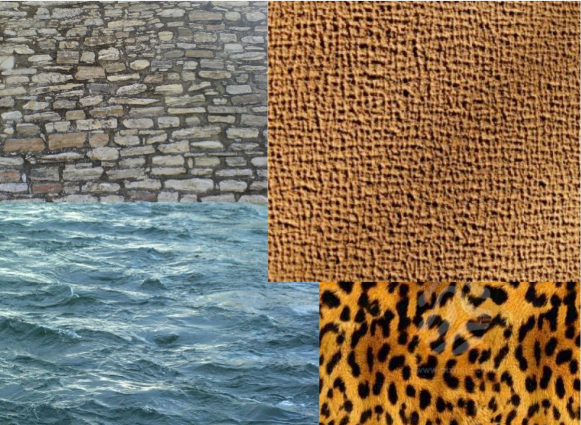
Figure 3.3: Stochastic textures

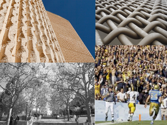
Figure 3.5: Interplay of texture and scale. Whether something is a texture depends on scale, and “structures” can appear and disappear across scales. Such “transitions” can be established in an ad-hoc manner using complexity measures as in Figure 3.6, or they can be established unequivocally by analyzing multiple views of the same scene through the notion of proper sampling, introduced in Section 5.1.

The concept of stationarity can be generalized from simple translation invariance to invariance relative to some group: In Figure 3.5 (top) the images do not have homogeneous statistics; however, in most cases one can apply an invertible transformation to the images that yields spatially homogeneous statistics.

The following characterization of texture is adapted from [63], where the basic definitions of stationarity, ergodicity, and Markov sufficient statistics are described in some detail. The important issue for us is that, if a process is stationary and ergodic, a statistic $\phi$ can be predicted from a realization of the image in some region $\bar{\omega}$. Once established that a process is stationary, hence spatially predictable, we can inquire on the existence of a statistic that is sufficient to perform the prediction. This is captured by the concept of Markovianity:

$$I(x)\perp I_{|_{{\omega}^{c}}}~{}|~{}\phi_{\omega\backslash x}.$$ (3.23)

Equation (3.23) establishes $\phi_{{\omega}}$ as a Markov sufficient statistic. In general, there will be many regions $\omega$ that satisfy this condition; the one with the smallest area $|\omega|=r$, determines a minimal sufficient statistic and the statistic defined on it is the elementary texture element. From now on, we will refer to $\phi_{\omega}$ as the minimal Markov sufficient statistic.

We can then define a texture as a region of an image that can be rectified into a sample of a stochastic process of a planar lattice that is locally stationary, ergodic and Markovian. More precisely, assuming for simplicity the trivial (translation) group, a region $\Omega\subset D\subset\mathbb{R}^{2}$ of an image is a texture at scale $\sigma>0$ if there exist regions $\omega\subset\bar{\omega}\subset\Omega$ such that $I$ is a realization of a stationary, ergodic, Markovian process locally within $\Omega$, with $I_{|_{\omega}}$ a Markov sufficient statistic and $\sigma=|\bar{\omega}|$ the stationarity scale. We then have that

$$H(I(x)|\omega-\{x\})=H(I(x)|\Omega-\{x\}).$$ (3.24)

We can therefore seek for $\omega\subset\Omega$ that satisfies the above condition. Without a complexity constraint, there are many regions that satisfy the above condition. To find $\omega$, we therefore seek for the smallest one, by solving

$$\hat{\omega}=\arg\min_{\omega}H(I(x)|\omega-\{x\})+\frac{1}{\beta}|\omega|.$$ (3.25)

Note that this is a consequence of the Markovian assumption and the Markov sufficient statistic satisfies the Information Bottleneck principle [173] with $\beta\rightarrow\infty$. As a special case, we can choose $\bar{\omega}$ to belong to a parametric class of functions, for instance square neighborhoods of $x$, excluding $x$ itself, of a certain size $\sigma$, ${\cal B}_{\sigma}(x)$, so the optimization above is only with respect to the positive scalar $\sigma$. The tradeoff will naturally settle for $1<r<\sigma$. Therefore, we can simultaneously infer both $\sigma$ and $r$ by minimizing the sample version of (3.25) with a complexity cost on $\sigma=|\bar{\omega}|$:

$$\hat{\omega},\sigma=\arg\min_{\omega,\sigma=|\bar{\omega}|}\hat{H}(I(x)|\omega-\{x\})+\frac{1}{\beta}|\bar{\omega}|.$$ (3.26)

Note that both $\omega$ and $\bar{\omega}$ are necessary for extrapolation: $\omega$ defines the Markov neighborhood used for comparing samples, and $\bar{\omega}$ defines the region where such samples are sought to approximate the probability distribution $p(I(x)|\omega-\{x\})$.

Eq. (3.26) provides means to infer both the Markov sufficient statistic as well as the scale $\sigma=|\bar{\omega}|$ of a texture, assuming that the stationarity and ergodicity assumptions are satisfied. Testing for stationarity (ergodicity must be assumed and cannot be validated) amounts to inferring $\Omega$, a texture segmentation problem. Estimating the group element $g\in G$ amounts to a canonization, or alignment process [3].

Given $\{I(x),x\in\Omega\}$, compression is achieved by inferring the (approximate) minimal sufficient statistic $\omega$ and the stationarity scale $\sigma$ by solving (3.26). Then $I(\bar{\omega})$, for any $\bar{\omega}\subset\Omega$ with $|\bar{\omega}|=\sigma$ is stored.

Given a compressed representation $I(\bar{\omega})$, we can in principle synthesize novel instances of the texture by sampling from $dP(I_{|_{\omega}})$ within $\bar{\omega}$. In a non-parametric setting this is done by sampling directly neighborhoods $I(\omega)$ within $\bar{\omega}$. To extrapolate the texture from a given sample $I(\bar{\omega})$ compatibility conditions have to be ensured at the boundaries of $\bar{\omega}$.

To find $\Omega$ we can solve

$$\Omega=\arg\min_{\bar{\omega}}H(I(x\in\partial\bar{\omega})|\bar{\omega})+\frac{\beta}{|\bar{\omega}|}$$ (3.27)

where the entropy is normalized by the length of the boundary $|\partial\bar{\omega}|$ (entropy rate). Since we do not know the distribution outside $\bar{\omega}$, the above is approximated by

$$\Omega=\arg\min_{\bar{\omega}}\hat{H}(I(x\in\partial\bar{\omega})|\bar{\omega},\hat{I}(x\in\delta\bar{\omega}-\{x\}))+\frac{\beta}{|\bar{\omega}|}.$$ (3.28)

In the continuum, the problem above can be solved using variational optimization as in [168]. In the discrete, the reader can refer to [63] for a description of compression, synthesis, segmentation and rectification algorithms.

3.5.2 Textures and Structures

In this section we establish the relation between textures, defined in the previous section, and structures, defined by co-variant detectors. Consider a point $x\in D$ and its neighborhood. If it is canonizable at a scale $\epsilon$, there is a co-variant detector with support $\epsilon$ (a statistic) that has an isolated extremum. This implies that the underlying process is not stationary at the scale $|\bar{\omega}|=\epsilon$. Therefore, it is not a texture. It also implies that any region $\omega$ of size $\epsilon=|\omega|$ is not sufficient to predict the image outside that region. This of course does not prevent a region that is canonizable at $\epsilon$ to be a texture at a scale $\sigma\neq\epsilon$. Within a region $\sigma$ there may be multiple frames of size $\epsilon$, spatially distributed in a way that is stationary/Markovian, so the region may be a texture at a scale $\sigma>\epsilon$. Vice-versa, if a region of an image is a texture with $\sigma=\bar{\omega}$, it cannot have a unique (isolated) extremum within $\bar{\omega}$, lest it would not be a sample of a stationary process. Of course, it could have multiple extrema, each isolated within a region of size $\epsilon<\sigma$. The above argument is a sketch of a proof of the following:

Theorem 4 (Structure-Texture)

For any given scale of observation $\sigma$, a region $\bar{\omega}$ with $|\bar{\omega}|=\sigma$ is either a structure or a texture.

Hence one can detect textures for each scale, as the residual of the canonization process described in the earlier part of this chapter. One may have to impose boundary conditions so that the texture regions fill around structure regions seamlessly. This can be accomplished by an explicit generative model that enforces boundary conditions and matches marginal statistics in the texture regions, following [85], as illustrated by [205]. However, this has to be done across all scales, unlike [205], since whether a region is classified as texture or structure depends critically on the scale $\sigma$.

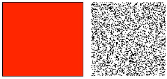
Figure 3.4: Testing the definition of texture. Both images above satisfy the definition of texture. Images like the one on the left, however, are often called “textureless.” Therefore, textureless is a limiting case of a trivial texture where any statistic $\phi$, computed in any region $\omega$, is constant with respect to any group $G$. Images like the one on the right are called random-dot displays, and Julesz showed that one can establish binocular correspondence between such displays (see Figure 5.2).

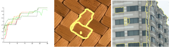
Figure 3.6: Texture-structure transitions (from [23]). The left plot shows the entropy profile for each of the regions marked with yellow boundaries in the middle and right figure. The abscissa is the scale of the region where such entropy is computed, starting from a point and ending with the entire image. As it can be seen, the entropy profile exhibits a staircase-like behavior, with each plateau bounded below by the scale corresponding to the small $\omega$, and above by the boundary of $\cal B$. This also shows that the neighborhood of a given point can be interpreted as texture at some scales (all the scales corresponding to flat plateaus), structure at some other scale (the non-flat transitions), then texture again, then structure again etc.

Remark 8 (“Stripe” textures)

The reader versed in low-level vision will notice that edges are not canonizable with respect to the groups we have discussed so far, including the translation group. This should come at no surprise, as we have anticipated in Remark 4, because of the aperture problem: While one can fix translation along the direction normal to the edge (at a given scale), one cannot fix translation along the edge (Figure 3.7). However, if one considers the sub-group of translations normal to the edge, the corresponding region is indeed canonizable.

Figure 3.7: The aperture problem: Locally, in a ball of radius $\sigma$, ${\cal B}_{\sigma}$, motion can only be determined in the direction of the non-zero gradient of the image. The component of motion parallel to an edge cannot be determined. This causes several visual illusions, including the so-called “barber pole” effect where a rotating cylinder appears to translate upward.

Since the decision of what is a structure depends on time (or, more in general, on the presence of multiple images), consequently, what is a texture is also a decision that requires multiple images. For instance, a random-dot stereogram [92] is everywhere canonizable and properly sampled at some scale $\sigma$, since one can establish correspondence. It is, however, a texture at all coarser scales, where any statistic is translation invariant.

The “random-dot display” of Figure 3.4 (right) seems to provide a counter-example to Theorem 4. In fact, Julesz [92] showed that random-dot displays can be successfully fused binocularly, which means that pixel-to-pixel correspondence can be established, which means the the image is canonizable at every pixel which, by Theorem 4, means that it is not a texture. But the random-dot display satisfies the definition of texture given in the previous section. How can this be explained?

First, there is no contradiction, since random-dot displays are indeed canonizable at the scale of the pixels $\sigma=1$. However, they are stationary at any coarser scale, hence they are textures at those scales.

More importantly, however, whether two regions of an image can be matched at a given scale depends not only on whether they are canonizable, but also whether they are properly sampled at that scale. We have anticipated the concept of proper sampling in Remark 6, and we will introduce and discuss the notion of proper sampling in Section 5.2, where we will revisit the random-dot display. There, we will see that the critical scales within which regions can be successfully matched (hence not called “textures” per Theorem 4) cannot be decided by analyzing one image alone. Instead, the “thresholds” for the transition from “matchable” to “non-matchable” require having multiple images of the same scene available.

Chapter 4 Designing feature detectors

Section 3.4 showed that rotation and contrast can be canonized, and that translation and scale can only be locally canonized. The definition of a canonized feature requires the choice of a functional $\psi$ (a co-variant detector), and an invariant statistic $\phi$ (a feature descriptor). Here we will focus on the location-scale group $g=\{x,\sigma\}\subset\mathbb{R}^{2}\times\mathbb{R}^{+}$, assuming that rotation and contrast have been canonized separately (later we advocate using gravity as a global canonization reference for orientation). The goal, then, is to design functionals $\psi$ that satisfy the requirements in Definition 3 that they yield isolated critical points in $G$. At the same time, however, we want them to be “unaffected” as much as possible by other nuisances. Such “insensitivity” is captured by the notions of commutativity, stability, which we introduce next, and proper sampling, that we introduce in the next chapter.

4.1 Sensitivity of feature detectors

We consider two qualitatively different measures of sensitivity. Note that we use the (improper) term “stability” because it is most commonly used in the literature, even though there is no equilibrium involved, and therefore the proper system-theoretic nomenclature would really be sensitivity. We will start from the most common notion of bounded-input bounded-output stability.

Definition 7 (BIBO stability)

A $G$-covariant detector $\psi$ (Definition 3) is bounded-input bounded-ouput (BIBO) stable if small perturbations in the nuisance cause small perturbations in the canonical element. More precisely, $\forall\ \epsilon>0\ \exists\ \delta=\delta(\epsilon)$ such that for any perturbation $\delta\nu$ with $\|\delta\nu\|<\delta$ we have $\|\delta\hat{g}\|<\epsilon$.

Note that $\hat{g}$ is defined implicitly by the equation $\nabla\psi(I,\hat{g}(I))=0$, and a nuisance perturbation $\delta\nu$ causes an image perturbation $\delta I=\frac{\partial h}{\partial\nu}\delta\nu$. Therefore, we have from the Inverse Function theorem [71]

$$\delta\hat{g}=-|J_{\hat{g}}|^{-1}\frac{\partial h}{\partial\nu}\delta\nu\doteq K\delta\nu$$ (4.1)

where $J_{g}$ is the Jacobian (3.7) and $K$ is called the BIBO gain. As a consequence of the definition, $K<\infty$ is finite. The BIBO gain can be interpreted as the sensitivity of a detector with respect to a nuisance. Most existing feature detector approaches are BIBO stable with respect to simple nuisances. Indeed, we have the following

Theorem 5 (Covariant detectors are BIBO stable)

Any covariant detector is BIBO-stable with respect to noise and quantization.

Proof: Noise and quantization are additive, so we have $\frac{\partial h}{\partial\nu}\delta\nu=\delta\nu$, and the gain is just the inverse of the Jacobian determinant, $K=|J_{\hat{g}}|^{-1}$. Per the definition of co-variant detector, the Jacobian determinant is non-zero, so the gain is finite.

BIBO stability is reassuring, and it would seem that a near-zero gain is desirable, because it is “maximally (BIBO)-stable.” However, simple inspection of (4.1) shows that $K=0$ is not possible without knowledge of the “true signal.” In particular, this is the case for quantization, when the operator $\psi$ must include spatial averaging with respect to a shift-invariance kernel (low-pass, or anti-aliasing, filter). However, a non-zero BIBO gain is irrelevant for recognition, because it corresponds to an additive perturbation of the domain deformation (domain diffeomorphisms are a vector space), which is a nuisance to begin with (corresponding to changes of viewpoint [167]). On the other hand, structural instabilities are the plague of feature detectors. When the Jacobian is singular, $|J_{\nabla\psi}|\rightarrow 0$, we have a degenerate critical point, a catastrophic scenario [144] whereby a feature detector returns the wrong canonical frame.

Definition 8 (Structural Stability)

A $G$-covariant detector $\psi\ |\ \nabla\psi(I,\hat{g}(I))=0$ is Structurally Stable if small perturbations $\delta\nu$ preserve the rank of the Jacobian matrix:

$$\exists\ \delta>0\ |\ |J_{\hat{g}}|\neq 0\Rightarrow|J_{\hat{g}+\delta\hat{g}}|\neq 0~{}~{}\ \forall\ \delta\nu\ |\ \|\delta\nu\|\leq\delta$$ (4.2)

with $\delta\hat{g}$ given from (4.1).

In other words, a detector is structurally stable if small perturbations do not cause singularities in canonization. We define the maximum norm of the nuisance that does not cause a catastrophic change [144] in the detection mechanism the structural stability margin. This can serve as a score to rank features.

Definition 9 (Structural Stability Margin)

We call the largest $\delta$ that satisfies equation (4.2) the structural stability margin:

$$\delta^{*}=\sup\|\delta\nu\|~{}~{}~{}~{}|~{}~{}~{}~{}|J_{\hat{g}+K\delta\nu}|\neq 0$$ (4.3)

Example 5 (Structural stability for the translation-scale group)

Consider the set of images, approximated by a sum of Gaussians as described in Section B.2.1. The image is then represented by the centers of the Gaussians, $\mu_{i}$, their variance $\sigma_{i}^{2}$ and the amplitudes $\alpha_{i}$, so that $I(x)=\sum_{i}\alpha_{i}{\cal G}(x-\mu_{i};\sigma_{i}^{2})$. Consider a detection mechanism that finds the extrema $\hat{g}=\{\hat{x},\sigma\}$ of the image convolved with a Gaussian centered at $\hat{x}$, with standard deviation $\sigma$: $\psi(I,\hat{g})=I*\nabla{\cal G}(x-\hat{x};\sigma^{2})=0$. Among all extrema, consider the two $\hat{x}_{1},\hat{x}_{2}$ that are closest. Without loss of generality, modulo a re-ordering of the indices, let $\mu_{1}$ and $\mu_{2}$ be the “true” extrema of the original image. In general $\hat{x}_{1}\neq\mu_{1}$ and $\hat{x}_{2}\neq\mu_{2}$. Let the distance between $\mu_{1}$ and $\mu_{2}$ be $d=|\mu_{2}-\mu_{1}|$, and the distance between the detected extrema be $\hat{d}=|\hat{x}_{2}-\hat{x}_{1}|$. Translation nuisances along the image plane do not alter the structural properties of the detector ($\hat{d}$ does not change). However, translation nuisance orthogonal to the image plane do. These can be represented by the scaling group $\sigma$, and in general $\hat{d}=\hat{d}(\sigma)$ is a function of $\sigma$ that starts at $\hat{d}=d$ when $\sigma=0$ and becomes $\hat{d}=0$ when $\sigma=\sigma^{*}$, i.e. when the two extrema merge in the scale-space. In this case, $\delta^{*}=\sigma^{*}$ is the structural stability margin. It can be computed analytically for simple cases of Gaussian sums, or it can be visualized as customary in the scale-space literature. It is the maximum perturbation that can be applied to a nuisance that does not produce bifurcations in the detection mechanism (Figure 4.1). Note that one could also compute the structural stability margin using Morse’s Lemma, or the statistics of the detector (e.g. the second-moment matrix). Finally, the literature on Persistent Topology [54, 40, 37] also provides methods to quantify the life-span of structures, which can be used as a proxy of the structural stability margin. Indeed, the notion of structural stability proposed above is a special case of persistent topology.

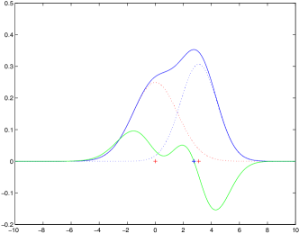
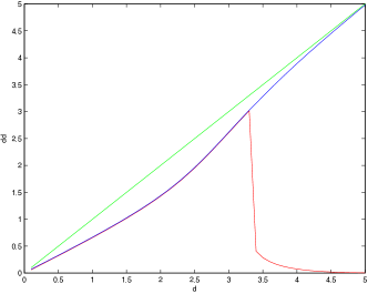
Figure 4.1: Catastrophic approximation: The original data is the sum of two Gaussians, one centered at $\mu_{1}=0$ (left, red dotted line), the other at a distance $\mu_{2}=d$ (left, blue dotted line) that increases from $0$ to $5$ (green line). The translation-detector $\hat{x}$ initially detects one extremum whose position (blue) deviates from $\mu_{2}$ as $d$ increases. However, at a certain point the detector $\hat{x}$ splits into two, $\hat{x}_{2}$ that follows $\mu_{2}$, and $\hat{x}_{1}$ that converges towards $\mu_{1}=0$. Note that at no point does the translation detector $\hat{x}$ coincide with the actual modes $\mu$ (i.e. , this detector is not BIBO insensitive). Furthermore, only for sufficiently separated, or sufficiently close, extrema does the location of the detector approximate the location of the actual extrema.

A sound feature detector is one that identifies Morse critical points in $G$ that are as far as possible from singularities. Structural instabilities correspond to aliasing errors, or improper sampling (Section 5.1), where spurious extrema in the detector $\psi$ arise that do not correspond to extrema in the underlying signal. Proper sampling depends on the detector functional $\psi$, that in the presence of quantization depends on the scale $\sigma$ (the area of the support of the quantization kernel). Thus the ideal detector is one that chooses $\hat{g}$ that is as far as possible from singularities in the locus $\{\hat{g}\ |\nabla\psi(I,\hat{g})=0\}$. The selection of the best canonical frames according to this principle is described in Section 5.2.

Note that a canonical frame $\hat{g}$ is often called a “feature point” or “keypoint” (or “corner”), an inappropriate nomenclature unless $G$ is restricted to the translation group. Note also that one should not confuse a (canonical reference) frame $\hat{g}$ from a (video) frame, which is an image $I_{t}$ that is part of a sequence $\{I_{t}\}_{t=1}^{T}$ obtained sequentially in time. Which “frame” we are referring to should be clear from the context.

Structural instabilities would be fatal if one insisted on uniqueness of the canonical element. However, as we have pointed out, occlusions prevent uniqueness in the first place; instead, we will have to select multiple canonical elements, each of which will have to be validated. Thus, in a sense, canonization is just a way of sampling the similarity group in a manner that is adapted to the signal, as opposed to being generic.

4.2 Maximum stability and linear detectors

In this section, as a way of example, we introduce detectors designed to be maximally BIBO stable. In other words, we look for classes of functionals $\psi$ that yield maximally isolated critical points. This seems to be an intuitive appealing criterion to follow. However, we will see in Section 5.1 that this does not guarantee structural stability. Nevertheless, we describe this approach because it is one of the most common in the literature, and it is better than just testing for the transversality condition (3.7), which is fragile in the sense that, in the presence of noise, it will almost always be satisfied. In Section 5.1 we will introduce an approach to feature detection that is better suited to the notion of structural stability. Therefore, the reader can skip this section unless he or she is interested in understanding the relation between the approach proposed there and the ones used in the current literature.

To design a maximally BIBO-stable detector, we look for functionals that yield critical points where the Jacobian determinant is not just non-zero, but it is largest. Following the most common approaches in the literature, we try to capture this notion using differential operators. In this case, we look for points that are at the same time zeros of $\nabla\psi\doteq\Psi$, and also critical points of $|\nabla\Psi|$. Now, in general, for a given class $\Psi$, there is no guarantee that the first set (zeros of $\Psi$) intersects the second (zeros of $\nabla|\nabla\Psi|$). However, we can look for classes of functions where this is the case, for all possible images $I$. These will be functionals that satisfy the following partial differential equation (PDE):

$$\Psi=\nabla|\nabla\Psi|.$$ (4.4)

Note that designing feature detectors by finding extrema of functionals requires continuity, which is something digital images do not possess. However, instead of finding extrema of the (discontinuous) image one can find extrema of operators, exploiting a duality as customary [41, 109, 170] especially for translation-invariance. Note that the “shift-plus-average” in [41] corresponds to template blurring, a lossy process that is not equivalent to proper marginalization or extremization.

We can start our quest for such functionals among linear ones, i.e. of the form $\Psi(I,\{x,\sigma\})={\cal G}*I(x,\sigma)=[0,0,0]^{T}$, where $*$ is a convolution product. In particular, ${\cal G}$ can be thought of as the gradient of a scalar kernel $k:\mathbb{R}^{2}\times\mathbb{R}^{3}\rightarrow\mathbb{R}^{+};(x,\{y,\sigma\})\mapsto k(x-y;\sigma)$, acting on the image via a convolution $k*I(x,\sigma)\doteq\int k(x-y;\sigma)I(y)dy$, so the zeros of ${\cal G}*I$ are the critical points of $k*I$, so ${\cal G}\doteq\nabla k^{T}$:

$$\hat{g}=\{x,\sigma\}\ |\ \int(\nabla k^{T}(x-y;\sigma)I(y)dy\doteq{\cal G}(x,\sigma)*I=0.$$ (4.5)

Written in terms of $\cal G$, the PDE above becomes an integro-partial differential equation (I-PDE)

$${\cal G}*I=\nabla|\nabla{\cal G}*I|$$ (4.6)

a condition that should be satisfied for all $I\in{\cal I}$. Note that the condition is only required at the zero-level set, so technically speaking a solution of the entire (4.6) is not necessary. We can approximate a generic function $I$ with a linear combination of (basis) vectors $\{b_{i}(x)\}$, $I(x)=B(x)\alpha$, where $B(x)=[b_{1}(x),\dots,b_{N}(x)]$ are, for instance, a complete orthonormal basis, then the condition above has to be satisfied for all functions $b_{i}(x)$. Of the many choices of basis, we favor one that follows a result of Wiener [192], that states that any positive $L^{1}$ distribution can be approximated arbitrarily well with a positive combination of Gaussian kernels. So, $b_{i}(x)={\cal N}(x-x_{i};\sigma_{i})$ are Gaussian kernels centered at $x_{i}$ with standard deviation $\sigma_{i}$. Therefore, the condition above becomes

$${\cal G}*{\cal N}(x,\sigma)=\nabla|\nabla{\cal G}*{\cal N}(x,\sigma)|\ ~{}~{}~{}\forall\ (x,\sigma).$$ (4.7)

All the gradient operators can thus be transferred to the Gaussian kernel by linearity, and derivatives of Gaussian are products of Gaussians with Hermite polynomials, that form a complete orthonormal family in $L^{2}$. Using Jacobi’s formula for the gradient of the determinant of a function with respect to its elements, we get

$${\cal G}*{\cal N}(x,\sigma)={\rm trace}\left({\rm adj}({\cal G}*{\nabla\cal N}){\cal G}*D^{2}{\cal N}\right)$$ (4.8)

where $D^{2}$ denotes the Hessian matrix and $\rm adj$ is the adjugate matrix of co-factors (each element $i,j$ is the determinant of the minor obtained by removing row $i$ and column $j$). This is another way of looking at (4.4) and (4.6), but now as an ordinary (non-linear) functional equation in the unknown $\cal G$.

The equation (4.4) is related to Monge-Ampere’s equation in optimal transport; an approximation of the determinant of the Hessian has been used for a Gaussian Kernel in approximate form (using Haar wavelet bases and the Integral Image) in the SURF detector [18].

Example 6 (Harris’ corner revisited)

The discussion above legitimizes the use of Hessian-of-Gaussian operators for feature detection, for instance [18]. The Laplacian-of-Gaussian operator, used in the popular SIFT [114], can also be partially justified on the grounds of first-order approximation of the Hessian, as customary in Newton methods. The other popularly used detector, Harris’ corner detector, however, is not explained by the derivation above. In fact, note that Harris’ operator

$$H(I,0)\doteq|\int\nabla^{T}I\nabla(I)dx|-\lambda{\rm Trace}\left(\int\nabla^{T}I\nabla(I)dx\right)$$ (4.9)

is not a linear functional of the image. It is still possible, however, to define the canonizing operator

$$\psi(I,g)=H(I,g)$$ (4.10)

and verify whether it yields isolated critical points. This is laborious and not relevant in the context of our discussion. We only mention that, because $H$ is non-linear, it does not commute with quantization, and therefore it does not meet the conditions of a proper co-variant detector (it is not commutative). Instead, below we suggest a different procedure to detect corners (or, more in general, junctions) that also provides a canonization procedure.

4.3 Non-linear detectors and the segmentation tree

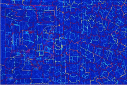
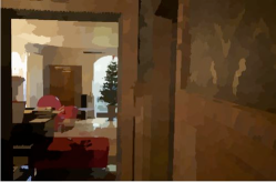
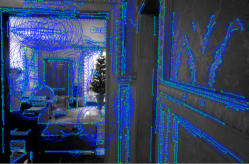
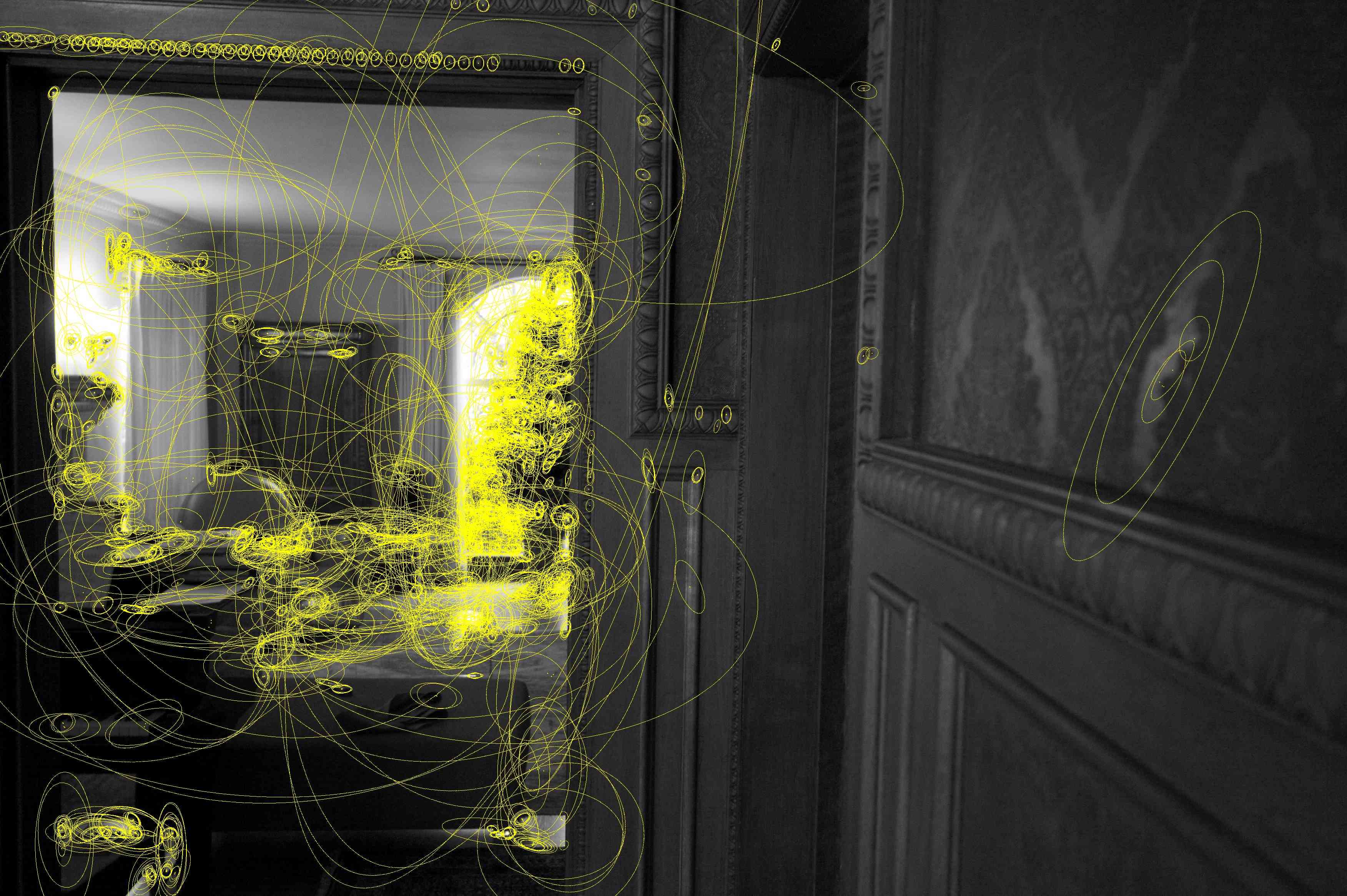
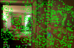
Figure 4.2: Representational structures: Superpixel tree (top), dimension-two structures (color/texture regions), dimension-one structures (edges, ridges), dimension-zero structures (Harris junctions, Difference-of-Gaussian blobs). Structures are computed at all scales, and a representative subset of (multiple) scales are selected based on the local extrema of their respective detector operators (scale is color-coded in the top figure, red=coarse, blue=fine). Only a fraction of the structures detected are visualized, for clarity purposes. All structures are supported on the Representational Graph, described in the next figure.

Linear functionals are not the only feature detectors. Indeed, Theorem 4 establishes the link between feature detection and (generalized) texture segmentation. Therefore, rather than testing for canonizability (as done customarily in feature detection) one can test for stationarity (as done customarily in segmentation) and then construct features from the segmentation tree. The caveat is that, because of the interplay of the scale group with quantization, and of the translation group with occlusion, no single segmentation can be used as a viable canonization procedure, and instead the entire segmentation tree must be considered.

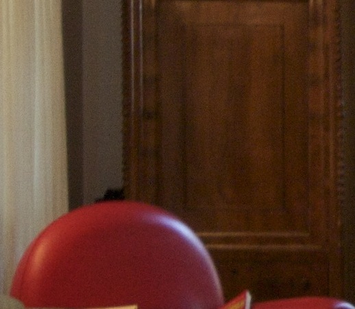
Figure 4.3: Representational Graph (detail, top-left) Texture Adjacency Graph (TAG, top-right); nodes encode (two-dimensional) region statistics (vector-quantized filter-response histograms), pairs of nodes, represented by graph edges, encode the likelihood computed by a multi-scale (one-dimensional) edge/ridge detector between two regions; pairs of edges and their closure (graph faces) represent (zero-dimensional) attributed points (junctions, blobs). For visualization purposes, the nodes are located at the centroid of the regions, and as a result the attributed point corresponding to a face may actually lie outside the face as visualized in the figure. This bears no consequence, as geometric information such as the location of point features is discounted in a viewpoint-invariant statistic.

The starting point for this approach to canonization is a different approximation model of the image. Rather than a linear combination of globally-defined basis vectors such as Gaussians or sinusoids, we use simple functions. These are constant functions on a compact domain, whose universal approximation properties in several measures are guaranteed by Weierstrass’ theorem [151]. In particular, let $\sigma>0$ be a given “scale.” Then, given an image, we can find a partition of the domain $D$ and constant values such that a combination of simple functions approximates the original image (or any statistic computed on it) to within $\sigma$ in each region (all filter channels can then be combined into a vector description of a region). Specifically, for a given $I\in{\cal I}$ and $\sigma$, we assume there is $N$ and constants $\{\alpha_{1},\dots,\alpha_{N}\}$ and a partition of the domain $\{S_{1},\dots,S_{N}\}$ such that

$$|I(x)-\alpha_{j}|\leq\sigma\ \forall\ x\in S_{j};~{}~{}~{}S_{i}\cap S_{j}=\delta_{ij};\ \cup_{j=1}^{N}S_{j}=D,$$ (4.11)

where $\delta_{ij}$ is Kronecker’s Delta. Then, if we define the simple functions as characteristic functions of $S_{j}$

$$\chi_{S_{j}}(x)=\begin{cases}1,\ \forall\ x\in S_{j}\\ 0\ {\rm otherwise}\end{cases}$$ (4.12)

we can approximate the image with

$$\hat{I}(x)=\sum_{j=1}^{N}\chi_{S_{j}}(x)\alpha_{j}.$$ (4.13)

This is true for scalar-valued images, but a similar construction can be followed to partition the domain into regions (often called superpixels), based on $\sigma$-constancy of any other statistic, such as color or any other higher-dimensional feature $\phi$. In any case, a superpixelization algorithm can be thought of as a quantizer, that is an operator that takes an image $I$ and a parameter $\sigma$ and returns a family of domain partitions $N=N(\sigma),\{\hat{S}_{j}\}_{j=1}^{N}$ with

$$\{\hat{S}_{j}\}_{j=1}^{N}=\phi_{\sigma}(I);~{}~{}~{}\hat{\alpha}_{j}=\frac{1}{|\hat{S}_{j}|}\int I(x)dx$$ (4.14)

where $|S_{j}|$ is the area of $S_{j}$. We can now use this functional to determine a co-variant detector $\psi(I,g)$. For the case of translation, $g=T$, we define (multiple) canonical elements $T_{j}$ to be the centroids of the regions $S_{j}$, $\hat{T}_{j}=\frac{1}{|S_{j}|}\int_{S_{j}}xdx$. Making the dependency on the image explicit, we have

$$\hat{T}(I,\sigma)=\frac{\int_{\phi_{\sigma}(I)}xdx}{\int_{\phi_{\sigma}(I)}dx}$$ (4.15)

to which there corresponds the canonizing functional

$$\psi(I,\{T,\sigma\})=\int_{\phi_{\sigma}(I)}xdx-T\int_{\phi_{\sigma}(I)}dx.$$ (4.16)

It can be easily verified that this functional is co-variant. For the case of translation (fixing $\sigma$), $g=T$, we have that, for $\hat{g}$ that solves $\psi(I,\hat{g})=0$, and for any $g$

$$\psi(I\circ g,\hat{g}\circ g) = \int_{\phi(I\circ g)}xdx-g\hat{g}\int_{\phi(I\circ g)}dx=\int_{g\phi(I)}xdx-g\hat{g}\int_{\phi(I)}dx=$$ (4.17)

$$= \int_{\phi(I)}gx^{\prime}dx^{\prime}-g\hat{g}\int_{\phi(I)}dx=g\left(\int_{\phi(I)}x^{\prime}dx^{\prime}-\hat{g}\int_{\phi(I)}dx\right)=$$

$$= g\psi(I,\hat{g})=0$$

where we have used the fact that the group $g$ is isometric, so $dx=dx^{\prime}$.

One may also believe that this functional yields isolated extrema, based on the fact that

$$|\nabla\psi|=|\frac{\partial\psi}{\partial T}|=\int_{\psi_{\sigma}(I)}dx>0.$$ (4.18)

However, this result, as well as (4.17), is misleading because it assumes that the superpixelization $\phi_{\sigma}(I)$ is independent of (small variations in) $T$. More precisely, in order for translation to be canonizable, the canonization process has to commute with quantization. If we assume that the underlying “ideal image” $I(x),\ x\in D$ is continuous, then the “discrete” (quantized) image $\hat{I}(x_{i})=\int_{{\cal B}_{\epsilon}(x_{i})}I(x)dx/\epsilon,x_{i}\in\Lambda$ defined on the lattice $\Lambda$, is related to it via the mean-value theorem, that guarantees the existence, for each $x_{i}$, of a translation $\delta_{i}$ such that

$$\hat{I}(x_{i})\doteq\frac{1}{|{\cal B}_{\epsilon}|}\int_{{\cal B}_{\epsilon}(x_{i})}I(x)dx=I(x_{i}+\delta_{i})=I(x_{i})+n_{i}\doteq I\circ\nu$$ (4.19)

where $\nu$ denotes the quantization nuisance. For the canonization process to be viable we must have

$$\phi_{\sigma}(I)=\phi_{\sigma}(I\circ\nu)$$ (4.20)

which is clearly not the case in general for a superpixelization algorithm. In fact, if we apply small perturbations to the levels $n_{i}$, from (4.19) we get small perturbations in the location of the boundaries $\partial S_{j}$, and in the location of their centroid, $T_{j}\rightarrow T_{j}+\delta_{i}$. Since $n_{i}=\nabla I(x_{i})\delta_{i}$, we see that for a superpixelization procedure $\phi_{\sigma}$ to provide a viable canonization mechanism, it has to place the boundaries in such a way that $\frac{\partial I}{\partial x}$ is negligible within each region, and as large as possible at region boundaries. We will see this spelled out more in detail shortly. The sensitivity of the boundary location as a function of a perturbation can be phrased in terms of BIBO stability, introduced in Definition 7. Specifically, if $\phi_{\sigma}$ is a quantization/superpixelization operator acting on an $\epsilon$-quantized image (4.19), and $\{S_{j}\}_{j=1}^{N}\doteq\phi_{\sigma}(I)$ and $\{\tilde{S}_{j}\}_{j=1}^{N}\doteq\phi_{\sigma}(I+n)$ the corresponding partitions, then $\phi_{\sigma}$ is BIBO stable if, according to (4.1),

$$\|n\|\leq\sigma\Rightarrow|\tilde{S}_{j}-S_{j}|\leq\epsilon$$ (4.21)

where $|S_{1}-S_{2}|$ denotes the area of the set-symmetric difference of the two sets $S_{1}$ and $S_{2}$.

Note that, in general, the operator $\phi_{\sigma}$ is not continuous, since it depends on $N$. When $N$ is fixed, it is possible to design a procedure that implements an operator $\phi_{\sigma}$ that is guaranteed to be stable even if the image is not continuous (but piece-wise differentiable). For instance, in a variational multi-phase region-based segmentation approach, one has an energy functional $E(I)$ that is continuous and minimized with respect to the (infinite-dimensional) partition $\{S_{j}\}$, so in this case we have that $\phi_{\sigma}$ is defined implicitly by the first-order optimality conditions (Euler-Lagrange) $\delta E(I)=0$, yielding a partial differential equation [168].

More in general, consider a perturbation of the image $\tilde{I}(x)=I(x)+n(x)$, with $n(x)$ assumed to be small in some norm. Then after quantization of the domain, using the Mean Value Theorem, we have

$$\tilde{I}(x_{i})=\int_{{\cal B}_{\epsilon}(x_{i})}\tilde{I}(x)dx=\int_{{\cal B}_{\epsilon}(x_{i})}I(x)dx+\int_{{\cal B}_{\epsilon}(x_{i})}\nabla I(x)dx\delta_{i}$$ (4.22)

where we have assumed that $\delta(x)$ is constant within each quantization region ${\cal B}_{\epsilon}(x_{i})$. Now, if we approximate the piecewise constant function in each ${\cal B}_{\epsilon}(x_{i})$ into a piecewise constant function in the partition $\{S_{j}\}_{j=1}^{N}$, for a given $N$, we have

$$\sum_{j=1}^{N}\chi_{\tilde{S}_{j}}(x_{i})\tilde{\alpha}_{j}=\sum_{j=1}^{N}\chi_{S_{j}}(x_{i})\alpha_{j}+\sum_{j=1}^{N}\chi_{S_{j}}(x_{i})\int_{{\cal B}_{\epsilon}(x_{i})}\nabla I(x)dx\delta(x_{i})$$ (4.23)

from which we can obtain, defining $\delta S_{j}=\tilde{S}_{j}-S_{j}$ the set-symmetric difference between corresponding regions, and measuring the area in each region,

$$\sum_{j=1}^{N}\sum_{x_{i}\in S_{j}}\chi_{\delta S_{j}}(x_{i})\alpha_{j}=\sum_{j=1}^{N}\int_{S_{j}}\nabla I(x)dx\delta_{j}$$ (4.24)

where we have now assumed that $\delta(x_{i})$ is constant within each $x_{i}\in S_{j}$, and we have called that constant $\delta_{j}$. So, we have that for a partitioning to be BIBO Stable, we must have

$$\sum_{j=1}^{N}|\delta S_{j}|\leq\sum_{j=1}^{N}\int_{S_{j}}\|\nabla I(x)\|dx$$ (4.25)

which is guaranteed so long as the image is smooth within each region $S_{j}$ (but it can be discontinuous across the boundary $\partial S_{j}$). Indeed, any reasonable segmentation procedure would attempt, for any given (fixed) $N$, to place the discontinuities of the (true underlying) image $I$ at the boundaries $\partial S_{j}$, therefore guaranteeing stability of the boundaries with respect to small perturbations of the image per the argument above. In particular, for $N=2$, there are algorithms that guarantee a globally optimal solution [35] that is, by construction, the most stable with respect to small perturbations of the image. These results are summarized into the following statement.

Theorem 6 (BIBO Stability of the segmentation tree)

A quantization/superpixelization operator, acting on a piecewise smooth underlying field and subject to additive noise, is BIBO stable at a fixed scale for a fixed tolerance $\delta$ (or complexity level $N$) if and only if it places the boundary of the quantized regions/superpixels at the discontinuities of the underlying field.

However, our concern is not just stability with respect to the partition $\{S_{j}\}_{j=1}^{N}$ for a fixed $N$, but also stability with respect to singular perturbations [43] that change the cardinality of the partition (a phenomenon linked to scale since $N=N(\sigma)$). So, the superpixelization procedure should be designed to be stable with respect to $N$, which is not a test we can write in terms of differential operations on the image. However, one can construct a greedy method that is designed to be stable with respect to both regular (bounded) and singular perturbations.

1. Start at level $k=0$ with each pixel representing as a region, $S_{i}(0)={\cal B}_{\epsilon}(x_{i})$ with $i=1,\dots,N_{0}=\#\Lambda$, the number of pixels in the image.

2. Construct a tree by creating a node representing the merging of the two regions that have the smallest average gradient along their shared boundary: for each $k$, obtain a new merged region $S_{i}(k+1)=S_{i_{1}}(k)\cap S_{i_{1}}(k)$ where

   $$i_{1},i_{2}=\arg\min_{l,m\ |\ S_{i}(j)\subset S_{l}(k)\cup S_{m}(k)}E_{l,m}(k)\doteq\\ \doteq\int_{\partial S_{l}(k)\cap\partial S_{m}(k)}\|\nabla I(x)\|dx/\int_{\partial S_{l}(k)\cap\partial S_{m}(k)}ds$$ (4.26)

3. Continue until the gradient between regions being merged fails the test (4.1), that is

   $$\hat{k},\hat{l}=\arg\min_{l,m}E_{l,m}(k)\geq\sigma.$$ (4.27)

4. At the end of the procedure, we have $N=N(\sigma)=N_{0}-k$ regions.

   These regions are, by construction, BIBO stable for any given value of $N$. Now to obtain a partition that is also stable with respect to singular perturbations, we have to choose regions that are unaffected by changes in $N$. To this end:

5. Consider each pixel $S_{i}(0)$, and follow its path in the tree, $\{S_{i}(k)\}$ as it is merged with other regions, together with the cost of each merging. Note that the cost is zero except when a merging occurs; call the mergings $\{k_{i_{1}},k_{i_{2}},\dots\}$. If at a certain $k_{i}$ we have that $S_{i}(k_{i})=S_{l}(k_{i})\cap S_{m}(k_{i})$, then the cost is $E_{i}(k_{i})\doteq E_{l,m}(k_{i})$ given by (4.27).

6. Let $\{k_{1}(i),k_{2}(i),\dots\}$ be the instances when the region $S_{i}$ is merged with one of its neighbors, and $E_{i}(k_{j}(i))$ the corresponding costs. Furthermore, let $\delta k_{j}(i)\doteq k_{j+1}(i)-k_{j}(i)$ be the “iteration gaps” between two merges involving the region $S_{i}$.

7. For each pixel $i$ and each set of indices $\{k_{i_{j}}\}_{j=1}^{L}$ sort the gaps $\delta k_{j}(i)\doteq k_{i_{j}}-k_{i_{j-1}}$ in decreasing order of their minimum gap

   $$\min(\delta k_{j}(i),\delta k_{j+1}(i)).$$ (4.28)

   The level $\hat{k}$ with the largest minimum gap corresponds to the region $S_{i}(\hat{k})$ containing the pixel $x_{i}$ that is least affected by singular perturbations. Indeed, for all $k_{j}(i)\leq k\leq k_{j+1}(i)$, any singular perturbation is a change in the value of $N=N_{0}-k$ that does not change the region $S_{i}(k)$.

If we follow this procedure for every pixel $i$, sorting their paths in decreasing order of gaps, until a minimum gap $\sigma$ is reached, then we have that each initial region $S_{i}(0)$ is now included in a number of (overlapping) regions $S_{i}(k_{j}(i))$ that are not only BIBO stable, but also stable with respect to singular perturbations. This follows by construction and is summarized in the following statement.

Theorem 7 (Stable segments)

Let $S_{i}(0)$, with $i=1,\dots,N_{0}$ be each pixel in an image. Then let $\{k_{j}(i)\}_{i,j}$ be ($j$-multiple) indices where $S_{i}$ is merged with neighboring regions,

$$k_{j}(i)=\arg\min_{l,m\ |S_{i}(k-1)\subset S_{l}(k-1)\cap S_{m}(k-1)}E_{l,m}(k)\leq\sigma$$ (4.29)

then the regions $\{S_{i}(k_{j}(i))\}_{i=1}^{N_{0}}$ are BIBO stable and stable with respect to singular perturbations.

Clearly many of these regions will be overlapping, and many indeed identical, so some heuristics can be devised to reduce the number of regions that, as it stands, can be more than the number of pixels in the image. A principle to guide such agglomeration is the so-called Agglomerative Information Bottleneck [61, 173].

This procedure relates to MSER [124], where however regions are created from the watershed, and are selected based on the variation of their boundary relative to their area as the watershed progresses. It also relates to other attempts to define “stable segmentations”, for instance [62]. However, in these cases stability is characterized empirically, and the algorithm is not guaranteed to be stable against a formal definition. Also, we are not necessarily interested in a partition of the domain, so long as a sufficient number of regions are present to enable local canonization.

So we have shown that canonizing translation via the centroid of superpixels is automatically viable, per (4.17) and (4.18), but only so long as the superpixelization is stable with respect to additive noise, for instance generated by quantization mechanisms.

Theorem 8 (Canonization via superpixels)

Let $\phi_{\sigma}(I)=\{S_{j}\}_{j=1}^{N}$ be a partition of the domain into superpixels. Then the functional (4.16) is a (local, translation) co-variant detector so long as it is BIBO stable.

That (4.16) is covariant follows from (4.17), provided that (4.1) is satisfied.

By the same token, one could canonize rotation by considering the principal axis of the sample covariance approximation of the regions $S_{j}$. Although [162] advocates canonizing general viewpoint changes by considering only the adjacency graph of the regions $S_{j}$, as we have discussed in Section 3, one should canonize no further.

An alternative (and dual) procedure for canonization is to use not the centroid of the superpixels, but their junctions, which are the points of intersection of the boundaries of adjacent superpixels. This provides a “corner detection mechanism” that is consistent with the theory, and can be used as an alternative to Harris’ corner detector discussed in the previous section. It should be noted that critical point filters [158] have been proposed for the detection of junctions at multiple scales.

Detection and canonization are not important per se, and can be forgone if one is willing to marginalize nuisances at decision time. Simple (conservative) detection can be thought of as a way not to select canonizable regions, but to quickly reject obviously non-canonizable ones. In this, the approach can be related to Boosting [60]. Where detection becomes important is when no marginalization can be performed, for instance in two adjacent frames in video, where one knows that the underlying scene is the same. As it turn out, this impoverished recognition problem, often called tracking, plays an important role in recognition, to the point where we devote a chapter to it, the next.

Before moving on, however, we would like to re-iterate the fact that the best mechanisms to eliminate nuisances is via marginalization or max-out. When decision-time constraints dictate that this is not feasible, canonization provides a useful way to reduce complexity, ideally keeping the expected risk in the overall decision problem unchanged (Section 2.4.1).

Chapter 5 Correspondence

In this chapter we explore the critical role that multiple images play in visual decisions. “Correspondence” refers to a particular case of visual decision problem, whereby two adjacent images are assumed to portray the same scene (owing to the physical constraints of causality and inertia, the scene is not likely to change abruptly from one image to the next), and this “bit” is used to prime the construction of models of the scene for recognition. Whether correspondence can be established depends on a variety of conditions that we describe next.

In the next section we will introduce the notion of Proper Sampling, that has been anticipated in Chapter 3, and is illustrated in Figure 5.1: A signal can be canonizable, but not properly sampled (i.e. , canonizability arises from aliasing effects, such as the block-structure due to quantization). Or, it can be properly sampled, but not canonizable (e.g. a constant region of the image), it can be not canonizable, and not properly sampled (e.g. a spatially and temporally independent realization of Gaussian “noise”), and finally it can be properly sampled and canonizable, for instance a “blob” or the fine-scale structure in a random-dot stereogram (Figure 5.2), not to be confused with “noise.”

Figure 5.1: A region of an image can be canonizable, but not properly sampled (left), or properly sampled, but not canonizable (right). Only when a region of the image is both properly sampled and canonizable can we establish meaningful correspondence between structures in the image and structures in the scene.

In Chapter 3 we have seen that an invariant descriptor can be constructed via canonization, but canonizability is a necessary, not sufficient, condition for meaningful correspondence. In order to be meaningful, a structure on the image needs to correspond to a structure in the scene, as we discussed in Remark 6. Unfortunately, this condition cannot be tested on one image alone. It can either be determined at decision time, by marginalization or extremization, or it can be determined – under the Lambertian assumption – by looking at different images of the same scene, as we describe next.

5.1 Proper Sampling

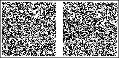
Figure 5.2: Texture or structure? This image helps understanding the importance of the notion of “proper sampling.” Since it is possible to fuse these two images in the random-dot stereogram binocularly and get a dense depth map [92], this means that point-to-point correspondence is possible, which would not be possible if this were a texture at the pixel scale, according to the definition in Section 3.5. However, the important question for correspondence is not whether something is a texture (stationary) or structure (canonizable), but whether it is properly sampled. This cannot be decided in a single image, but by testing the proper sampling hypothesis of Definition 10. In the specific case of the random-dot stereogram, this is a properly sampled pair of images, that just happen to have a very complex radiance. Recall that proper sampling depends not just on the scene, but also on the imaging condition, including the distance from the scene and the point-spread function of the eye, both of which affect the scale of the representation.

Feature detection is a form of sampling, but one that is rather different from the classical sampling theory of Nyquist and Shannon. In traditional signal processing, proper sampling refers to regular sampling at twice the Nyquist rate, since a band-limited signal can be reconstructed exactly from the samples under these conditions. This assumes that the signal is band-limited, which is as much an idealization as the Lambert-Ambient static model (strictly band-limited signals do not exist, as they would have to have infinite spatial support).

But we are not interested in using the data to reconstruct a replica of the “original signal.” Instead, we are interested in using the data to solve a decision or control task as if we had the “original signal” at hand. But what is the “original signal” in our context? It is the image before any quantization phenomena occur. For a single image, since we cannot detect occlusions (Section 8.1), quantization represents the main non-invertible nuisance (neglecting complex illumination effects). Similarly, as we have seen in Theorem 3, the translation-scale group $g=\{x,\sigma\}$ is the main invertible nuisance (since more complex groups are not invertible once composed with quantization). Therefore, following (2.8) in Section 2.2, we have that if the image is $I=h(g,\xi,\nu)+n$, then the “ideal image” is

$$h(e,\xi,0)\doteq\rho(\pi^{-1}(D)).$$ (5.1)

Therefore, in the context of visual decisions, we can define proper sampling as a discretization that yields a response of co-variant detector functionals having the same number, type and connectivity of critical points that the “ideal image” would produce.

Definition 10 (Proper Sampling)

A signal $I$ is properly sampled at a scale $\sigma$ if a co-variant detector operating on the image yields the same critical points as if it operated on the radiance of the scene. In other words, if $\psi(I,g)$ is a co-variant detector for the location-scale group $g=\{x,\sigma\}$, and $h(e,\xi,0)\doteq\rho\circ\pi^{-1}(D)$, then $\nabla\psi(I,\hat{g})=0\Leftrightarrow\nabla\psi(h(\hat{g},\xi,0))=0$, and corresponding extrema are of the same type.

In other words, an image is properly sampled if it is possible to reconstruct, from the samples, not the “ideal image” (the radiance of the scene), but one that is topologically equivalent to to it, in the sense of yielding the same extrema via a co-variant detector operator. The attributed Reeb tree (ART) is a topological construction that can be assembled from the image at any given scale. It is a tree with nodes at every isolated extremum (maxima, minima, saddles), with edges connecting extrema that are “adjacent” in the sense of the Morse-Smale complex. The value of the image at the extrema is not relevant, but the ordering is, and the position of these extrema is not relevant, but the connectivity is. The ART was introduced in [167] as a maximal contrast-viewpoint invariant away from occlusions, and is described in more detail in Section A.2. It can be shown that the outcome $\hat{g}=\{\hat{x}_{i},\sigma\}$ of any feature detector $\nabla\psi(I,\hat{g})=0$ operating at a scale $\sigma$ can be written in terms of the $ART$: $\{\hat{x}_{i}\}_{i=1}^{N}=ART(I*{\cal G}(x;\sigma^{2}))$, which leads to the following claim.

Theorem 9

A signal $I$ is properly sampled at $\sigma$ if and only if $ART(h(e,\xi,0)*{\cal G}(x;\sigma^{2}))=ART(I*{\cal G}(x;\sigma^{2}))$.

Thus, any of a number of efficient techniques for critical point detection [159] can be used to compute the $ART$ and test for proper sampling. Note that, in general, any feature detection mechanism alters the position of the extrema relative to the original signal, as illustrated in Example 5. This is not an issue in the context of visual decisions, because extrema move as a result of viewpoint changes, and their motion would therefore be discarded as a nuisance anyway.

The problem with the definition of proper sampling is that it requires knowledge of the “ideal image” $h(e,\xi,0)$, which is in general not available (indeed, it may be argued that it does not exist). Unlike classical sampling theory, there is no “critical frequency” beyond which one is guaranteed success in canonization, because of the scaling/quantization phenomenon. Therefore, to test for proper sampling on the image $I_{t}(x)$, rather than comparing it to the “ideal image”(which is a function of the unknown radiance distribution of the scene), we compare it to the next image $I_{t+1}(x)$, which is equivalent to it under the Lambertian assumption in the co-visible region [164], as done in Section 2.2. Therefore, the notion of proper sampling (now in space and time) relates to the notion of correspondence, co-detection, or “trackability” as we explain below.

Definition 11 (Proper Sampling)

We say that a signal $\{I_{t}\}_{t=1}^{T}$ can be properly sampled at scale $\sigma_{t}$ at time $t$ if there exists a scale $\sigma_{t+1}$ such that $ART(I_{t}*{\cal G}(x;\sigma_{t}^{2}))=ART(I_{t+1}*{\cal G}(x;\sigma_{t+1}^{2}))$.

In other words, a signal is properly sampled in space and time if the feature detection mechanism is topologically consistent in adjacent times. Alternatively, we can impose that $\sigma_{t}=\sigma_{t+1}$ and therefore require topological consistency at the same scale. Sometimes we refer to proper sampling of corresponding regions in two images as being co-canonizable.

Note that in the complete absence of motion, proper sampling cannot be ascertained. However, complete absence of motion is only real when one has one image, as a continuous capture device will always have some changes, for instance due to noise, making two adjacent images different, and therefore the notion of topological consistency over time meaningful, since extrema due to noise will not be consistent. Note that the position of extrema will in general change due to both the feature detection mechanism, and also the inter-frame motion. Again, what matters in the context of visual decisions is the structural integrity (stability) of the detection process, i.e. its topology, rather than the actual position (geometry). If a catastrophic event happens between time $t$ and $t+1$, for instance the fact that an extremum at scale $\sigma$ splits or merges with other extrema, then tracking cannot be performed, and instead the entire $ART$s have to be compared across all scales in a complete graph matching problem.

While establishing correspondence under these circumstances can certainly be done (witness the fact that we can recognize the top-left image in Figure 5.1 as a quantized photograph of Abraham Lincoln), this has to be done by marginalization, extremization or canonization, treating correspondence as a full-fledged recognition problem (a.k.a. wide-baseline matching) rather than exploiting knowledge that the underlying scene is the same. This is the crucial “bit” provided by temporal continuity. Motivated by this reasoning, we introduce the notion of “trackability.”

Definition 12 (Trackability)

A region of the image $I_{|_{\cal B}}$ is trackable at a given scale if it is canonizable and properly sampled at that scale.

It may seem at first that any region of an image can be made trackable by considering it at a sufficiently coarse scale. Unfortunately, this is not the case.

Remark 9 (Occlusions)

We first note that occlusions do, in general, alter the topology of the feature detection mechanism, hence the $ART$. Therefore, they cannot be properly sampled at any scale. This is not surprising: We know that we cannot track through an occlusion, as correspondence cannot be established for regions that are visible in one image (either $I_{t}$ or $I_{t+1}$) but not the other. In the context of feature detectors/descriptors, occlusion detection reduces to a combinatorial matching process at decision time. Pixel-level occlusion detection will be discussed in Section 8.1.

Remark 10

Note that a signal is not properly sampled per-se. In general, only trivial signals are globally properly sampled. However, there is a scale at which a signal may be properly sampled, as we will see shortly. As an illustration, Figure 5.3 shows the same image that is not properly sampled at the pixel level (left) but it is properly sampled when seen at a significantly coarser scale (small in-set image on the left, or blurred version on the right).

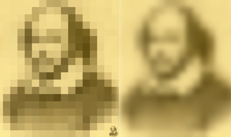
Figure 5.3: Whether an image is properly sampled depends on scale. The image on the left is not properly sampled at the finest scale afforded by the reproduction medium of this manuscript. However, it is properly sampled at a considerably coarser scale (right).

Note that the notion of proper sampling relates to texture, in the sense that even if two images independently exhibit stationary statistics (and therefore they are independently classified as textures), if they are co-canonizable they are properly sampled, and therefore point-correspondence can be established (Figure 5.2). Also, we recall that we consider constant-color regions to be (trivial) textures, even though they are often referred to as “textureless.” Note that a constant-intensity region is, in general, properly sampled, but not canonizable. A stochastic texture is not canonizable (by definition) at the native scale (sensor resolution), where it is usually not properly sampled, because canonizability arises from sampling/aliasing phenomena. Note, again, that all these considerations depend on scale, as we have discussed in Section 3.5. Also note that we are not assuming that the signals we measure are properly sampled. Instead, we use the definition to test the hypothesis of proper sampling at a given scale, and therefore determine co-visibility and ascertain trackability.

Although, as we have pointed out before, two-dimensional scale-spaces do not enjoy a causality property, typically the number of extrema diminishes at coarser scales, and the extrema that persist are, usually, corresponding to some structure in the image. So, although one cannot prove that for any image there exists a scale at which it can be properly sampled, in co-visible regions, one typically finds this to be the case for most natural images. This is because, at large enough scales, extrema will coalesce, and eventually quantization phenomena become negligible.

Therefore, one can conjecture that, for most natural images, in the absence of occlusions, assuming continuity and a sufficiently slow motion relative to the temporal sampling frequency, any image region is trackable. This means that there exists a large-enough scale $\sigma_{max}$ such that $ART(I_{t}*{\cal G}(x;\sigma_{max}^{2})=ART(I_{t+1}*{\cal G}(x;\sigma_{max}^{2})$.

Thus anti-aliasing in space can lead to proper sampling in time. This is important because, typically, temporal sampling is performed at a fixed rate, and we do not want to perform temporal anti-aliasing by artificially motion-blurring the images, as this would destroy spatial structures. Note, however, that once a large enough scale is found, so correspondence is established at the scale $\sigma_{max}$, the motion ${\hat{g}}_{t}$ computed at that scale can be compensated for, and therefore the (back-warped) images $I_{t}\circ{\hat{g}}^{-1}_{t}$ can now be properly sampled at a scale $\sigma\leq\sigma_{max}$. This procedure can be iterated, until a minimum $\sigma_{min}$ can be found beyond which there is no topological consistency. Note that $\sigma_{min}$ may be smaller than the native resolution of the sensor, leading to a super-resolution phenomenon.

This suggests a procedure for tracking, whereby one first selects structurally stable features via proper sampling. The structural stability margin determines the neighborhood in the next image where detection is to be performed. If the procedure yields precisely one detection in this neighborhood, topology is preserved, and proper spatio-temporal sampling is achieved, hence trackability. Otherwise, a topological change has occurred, and the track is broken. This procedure is performed first at the coarsest level, and then propagated at finer scales by compensating for the estimated motion, and then re-selecting at the finer scales [106]. Note that this procedure, described in more detail in the next section, is different from traditional multi-scale feature tracking, where each feature detected at the finest scale is tracked at all coarser scales. In this framework, feature detection is initiated at each scale, in the region back-warped from coarser scales.

5.2 The role of tracking in recognition

The goal of tracking is to provide correspondence of (similarity or isometric) reference frames $\hat{g}_{ij}=\{x_{i},\sigma_{ij},R_{ij}\}$, centered at $x_{i}$, with size $\sigma_{ij}$ and orientation $R_{ij}$. This is the outcome of feature detection based on structural stability and proper sampling. Because of temporal continuity, the class label $c$ is constant under the assumption of co-visibility and false otherwise. In this sense, time acts as a “supervisor” or a “labeling device” that provides ground-truth training data. The local frames $g_{k}$ are now effectively co-detected in adjacent images. Therefore, the notion of structural stability and “sufficient separation” of extrema depends not just on the spatial scale, but also on the temporal scale. For instance, if two $5$-pixel blobs are separated by $10$ pixels in one image, they are not sufficiently separated for tracking under temporal sampling that yields a $20$-pixel inter-frame displacement.

Thus the ability to track depends on proper sampling in both space and time. This suggests the approach to multi-scale tracking used in [106]:

1. Construct a spatial scale-space of feature detectors, until the signal is properly sampled in time.

2. Estimate motion at the coarser scale, with whatever feature tracking/motion estimation/optical flow algorithm one wishes to use [106]. This is now possible because the proper sampling condition is satisfied both in space and time.

3. Propagate the estimated motion in the region determined by the detector to the next scale. At the next scale, there may be only one selected region in the corresponding frame, or there may be more (or none), as there can be singular perturbations (bifurcations, births and deaths).

4. For each region selected at the next scale, repeat the process from 2.

This is illustrated in Figure 5.4.

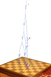
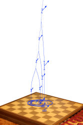
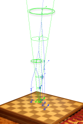
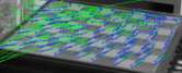
Figure 5.4: Tracking on the selection tree. The approach we advocate only provides motion estimates at the terminal branches (finest scale); the motion estimated at inner branches is used to back-warp the images so large motion would yield properly-sampled signals at finer scales (left). As an alternative, the motion estimated at inner branches can also be returned, together with their corresponding scale (middle). Traditional multi-scale detection and tracking, on the other hand, first “flattens” all selections down to the finest level (dashed vertical downwards lines), then for all these points considers the entire multi-scale cone above (shown only for one point for clarity). As a result, multiple extrema at inconsistent locations in scale-space are involved in providing coarse-scale initialization (right). Motion estimates at a scale finer than the native selection scale (thinner green ellipse), rather than improving the estimates, degrade them because of the contributions from spurious extrema (blue ellipses). Motion estimates are shown on the right (blue = [106], green = multi-scale Lucas-Kanade [116, 14]).

Note that only the terminal branches of the selection scale-space provide an estimate of the frame $\hat{g}$, whereas the hidden branches are used only to initialize the lower branches. Nevertheless, one can report each motion estimate at the native selection scale (Figure 5.4 middle), even if they are subsumed by the terminal branches of the selection tree.

This approach is called tracking on the selection tree (TST) [106], because it is based on proper sampling conditions and tracking is performed at each native selection scale. Indeed, note that the “second-moment-matrix” test commonly used for tracking [116, 176], even if performed at each scale, cannot be relied upon to reject features that cannot be tracked. This is because it is possible, and indeed typical, that due to singular perturbations, the region passes the second-moment test (e.g. harris’ [74]) at each scale, but not because the feature of interest is trackable, but because additional structures have appeared in the new scale (Figure 5.4 right). This is a form of structural aliasing phenomenon.

Tracking provides a time-indexed frame $\hat{g}_{t}$ that can be canonized in multiple images to provide samples of the canonized statistic $\phi^{\wedge}h(\xi,\nu_{t})$, where $\nu_{t}$ lumps all other nuisances that have not been canonized (including the group nuisances that do not commute with non-invertible nuisances). These can then be used to build a descriptor, for instance a template (2.30), or more general ones that we discuss next.

Note that the process of selection by maximizing the structural stability margin can be understood as a scale canonization process, even though in Section 3.4 we argued against canonization of scale. Note, however, that here we are not making an association of features across scales other than for the purpose of initializing tracks. In particular, consider the example of the corner in Figure 5.4: The corner only exists at the finest scale. Features detected at coarser scales serve to initialize tracking at the finest scale, but features selected at coarse scales are not associated to the corner point, they are simply different local features. Aggregating multiple TSTs can also be done, when some “side information” is available that enables to group them together. For instance, in [196], detachability is used as side information [10], exploiting, again, knowledge of occlusions [9].

Chapter 6 Designing feature descriptors

A feature detector provides a $G$-covariant reference frame, relative to which the image is, by construction, $G$-invariant. So, the simplest invariant descriptor is the image itself, expressed in the reference frame determined by the detector (3.8). For the case of Euclidean and contrast transformations, $G=SE(2)\times{\cal M}$, where $\cal M$ denotes the set of monotonic continuous transformations of the range of the image. In the case in which a sequence of images is available, correspondence of reference frames is provided by tracking $\{g_{t}\}_{t=1}^{T}$, as described in Section 5.1, and again the entire time series in the normalized frame, $I\circ g_{t}^{-1}$ is by construction $G$-invariant. Of course, all the non-invertible nuisances, as well as the group nuisances that do not commute with them, are not eliminated by this procedure, and therefore they have to be dealt with at decision time via either marginalization (2.12), or extremization (2.13). Using the formal image-formation model $h$, and the maximal $G$-invariant $\phi^{\wedge}$, we have that

$$\phi^{\wedge}(\{I_{t}\}_{t=1}^{T})=\{h({\hat{g}}^{-1}_{t}(I_{t}),\xi,\nu_{t})\}_{t=1}^{T}.$$ (6.1)

However, marginalizing or max-outing the residual effects of the nuisance $\{\nu_{t}\}_{t=1}^{T}$ – that include occlusions, quantization, noise, and all un-modeled photometric phenomena such as specularities, translucency, inter-reflections etc. – can be costly at decision time. Therefore, in Section 2.6.1, we have justified the introduction of an alternate approach that attempts to simplify the decision run-time by aggregating the training set into a template. Of course, one could do the same on the test set, which may consist of a single image $T=1$, or of video. The result is what is called a feature descriptor. In this chapter we will explore alternate descriptors, more general than the best template described in Section 2.6.1, which we show how to compute in Section 6.3. We also discuss relationships to sparse coding in Section 6.5, which links to the discussion of linear detectors in Section 4.2. Recall that the “best template” in Section 2.6.1 is only the best among (static) templates. Therefore in Section 6.4 we show that one can, in general, achieve better results by not eliminating the time variable $t$ as part of the feature description process, but retaining the time variable, and instead marginalizing it or max-outing it as part of the decision process. This requires the introduction of techniques to marginalize time, which we describe in Section 7.2.

Before doing all that, however, we summarize the role of various nuisances and how they are handled before the descriptor design process commences.

6.1 Nuisance taxonomy (summary)

This section summarizes material from previous chapters, and can therefore be skipped. In Section 2.2 we have divided the nuisance into those that have the structure of a group, $g$, and those that are non-invertible, $\nu$, including the additive component $n$, which we refer to as “noise.” Then, in Section 3.4, we have shown that of the group nuisance, only a sub-group commutes with $\nu$ and $n$. These are the group-commutative nuisances, consisting of the isometric group of the plane. Indeed, these are only locally canonizable and therefore can be eliminated at the outset via co-variant detection and invariant description (3.8), modulo a selection process corresponding to combinatorial matching at decision time, to marginalize the occlusion nuisance, as described in (3.20) in Section 3.4. In this section we elaborate on how to treat the various nuisances, thus expanding (3.20).

Translation:

Canonization corresponds to the selection of a particular point (feature detection) that is chosen as (translational) reference. The image in this new reference is, by construction, invariant to planar translation, assuming that the feature detection process is structurally stable, commutes with non-invertible nuisances, and there is no occlusion. There are many mechanisms to canonize translation. Examples include the extrema of the determinant of the Hessian of the image, or of the convolution with a Laplacian of Gaussian, extrema of the determinant of the second-moment matrix. In any case, one must choose multiple translations $T_{i}$ at each sample scale $\sigma_{j}$. As we have discussed in Section 4, scale should be sampled, not canonized (it does not commute with quantization), and it can be either sampled regularly, or adaptively in a way that yields maximum structural stability margins, as described in Section 4.1. If the image is encoded by a “segmentation tree” (a partition of the domain into regions that are constant to within a certain tolerance $\sigma$), then the centroid of each region (a node in the region adjacency graph) or the junctions of boundaries of three or more regions (faces in the adjacency graph) are also viable canonization procedures that can be designed to be structurally stable.

Scale:

Scale is not canonizable in the presence of quantization. Whatever descriptor one chooses should be represented at multiple scale. This is described in Section 5.2.

Note that a variety of sampling options is possible, depending on the interplay with translational feature detection. One could first sample all available scales, and then independently canonize translation in each one. Or, one could canonize translation at the native scale of the image, and then sample the image at multiple scales at that location. Or, one can simultaneously sample scale and detect translational frames by performing maximally-structurally stable translation selection, where the maximization of the stability margin is performed relative to scale. This is accomplished in a manner similar to scale selection as prescribed by [109], described in [106]. It is conceptually important to understand that multiple scales can be detected at the same location, therefore the scale selection process is more like an adaptive scale sampling as opposed to a (unique) scale canonization procedure.

Rotation:

Planar rotation is canonizable, and therefore it should be canonized. In the presence of measurements of gravity, a natural canonical orientation is provided by the projection of the gravity vector onto the image plane (assuming it is not aligned with the optical axis).

If we have $N_{T}N_{S}$ regions available from sampling translations and scale, we can canonize each one with a co-variant detector and its corresponding invariant descriptor $\phi_{R}$. Co-variant detection can be performed in a number of ways, using extrema of the gradient direction [114] (at each location, at each scale), or the principal direction of the second moment matrix [126] at each location and scale, or nodes and faces of the adjacency graph of $\epsilon$-constant regions [186], at each location and scale. The result is an unchanged number $N_{T}N_{S}$ of descriptors that are now invariant to rotation as well as (locally) translation. Alternatively, rotation can be canonized by using gravity and longitude (or latitude) as canonical references.

Contrast:

Contrast can be canonized independently of other nuisances by replacing the intensity at every pixel with the gradient direction:

$$\phi(I)=\frac{\nabla I}{\|\nabla I\|}.$$ (6.2)

This is conceptually straightforward, except that it assumes that the image is differentiable, which in general is not the case (one can define discrete differentiability which, however, entails a choice of scale, thus making this choice still dependent on scale). It also raises issues when $\|\nabla I\|=0$, i.e. , when the image is constant in a region. As an alternative mechanism, one can canonize contrast, in a local region determined by a translational frame $T_{i}$ at a scale $\sigma_{j}$, by normalizing the intensity by subtracting the mean and dividing by the standard deviation of the image, or of the logarithm of the image. If we call $B_{ij}\doteq{\cal B}_{\sigma_{j}}(x-T_{i})$ a neighborhood of size $\sigma_{j}$ around the canonical reference $T_{i}$, then

$$\phi_{ij}(I)=\frac{I-\mu(I)}{{\rm std}(I)}$$ (6.3)

where $\mu(I)\doteq\frac{\int_{B_{ij}}I(x)dx}{\int_{B_{ij}}dx}$ and ${\rm std}(I)\doteq\sqrt{\frac{\int_{B_{ij}}|I(x)-\mu(I)|^{2}dx}{\int_{B_{ij}}dx}}.$ In this latter case, the canonization procedure interacts with scale, and therefore contrast normalization should be done independently at all scales. Additional options if multiple spectral bands are available is to consider spectral ratios, for instance in an $(R,G,B)$ color space one can consider the ratio $R/B$ and $G/B$, or the normalized color space, or in an $(H,S,V)$ color space one can consider the $H$ and $S$ channels, etc.

Among the nuisances that cannot be canonized, in addition to scale and occlusion that should be sampled and marginalized as in Section 3.4, we have:

Illumination:

Complex illumination effects other than contrast cannot be canonized, and therefore their treatment should be deferred to decision time.

Quantization and noise:

Quantization is intertwined with scale and cannot be canonized. At each scale, quantization error can be lumped as additive noise. Detectors for canonizable nuisances should be designed to commute with quantization and noise. Linear detectors do so by construction.

Skew:

One could treat the (non-canonizable) group of skew transformation in the same way as scale, but since there is no meaningful sampling of this space, we lump the skew with other deformations and defer their treatment to marginalization or blurring.

Deformations and quantization:

Domain deformations other than rotations and translations, including the affine and projective group or more general diffeomorphisms, cannot be canonized in the presence of quantization, and therefore their handling should be deferred to either training (blurring) or testing (marginalization, extremization).

Occlusion:

Occlusions, finally, are not invertible and cannot be canonized, so they will have to be explicitly detected during the matching process (via max-out or marginalization), which in this case corresponds to a selection of a subset of the $N_{T}N_{S}$ local descriptors as described in Section 3.4.

What we have in the end, for each image $I$, is a set of multiple descriptors (or templates), one per each canonical translation and, for each translation, multiple scales, canonized with respect to rotation and contrast, but still dependent on deformations, complex illumination and occlusions:

$$\phi(I) = \{k_{ij}\circ\rho(S_{j}R_{ij}x+T_{i}+v_{ij}(x))+n_{ij}(x),$$

$$~{}~{}~{}~{}~{}i,j=1,\dots N_{T},N_{S}|{\cal B}_{\sigma_{j}}(x+T_{i})\cap D=\emptyset\}$$

where $v_{ij}$ is the residual of the diffeomorphism $w(x)$ after the similarity transformation $SRx+T$ has been applied, i.e. , $v_{ij}(x)=w(x)-S_{j}R_{ij}x-T_{i}$. Here $S=\sigma I$ is a scalar multiple of the identity matrix that represents an overall scaling of the coordinates, and $(R,T)\in SE(2)$ represent a rigid motion with rotation matrix $R\in SO(2)$ and translation vector $T\in\mathbb{R}^{2}$. If we call the frame determined by the detector $\hat{g}_{ij}=\{S_{j},T_{i},R_{ij},k_{ij}\}$, we have that

$$\phi(I)=\{I\circ{\hat{g}}^{-1}_{ij}\}_{i,j=1}^{N_{T},N_{S}}.$$ (6.5)

Note that the selection of occluded regions, which is excluded from the descriptor, is not known a-priori and will have to be determined as part of the matching process. As we have discussed in Section 4.1, the selection process should be designed to be invariant with respect to group-commutative nuisances, and “robust” (in the sense of structural stability) with respect to all other nuisances. The selection and tracking process described in Section 5.1 provides one such design.

In the case of video data, $\{I_{t}\}_{t=1}^{T}$, one obtains a time series of descriptors,

$$\phi(\{I_{t}\}_{t=1}^{T})=\{I_{t}\circ{\hat{g}}^{-1}_{ij}(t)\}_{i,j,t=1}^{N_{T},N_{S},T}$$ (6.6)

where the frames $\hat{g}_{ij}(t)$ are provided by the feature detection mechanism that, in the case of video, includes tracking via proper sampling (Section 5.1). Once that is done, one should store the time series of descriptors $\phi(\{I_{t}\}_{t=1}^{T})$ for later marginalization, if sufficient storage and computational power is available, as we describe in Section 6.4. Otherwise, a static descriptor can be devised, as we discuss in Section 6.3. Before doing so, however, we discuss the interplay between the scene and the nuisance in the next section.

6.2 Disentangling nuisances from the scene

In the image-formation model described in Section 2.2, and in the more general model in Section B.1, some of the nuisances interact with the scene to form an image. If the nuisances are marginalized or max-outed, as in (2.12) or (2.13), this is not a problem. However, if we want to canonize a nuisance, in the process of making the feature invariant to the nuisance, we may end up making it also invariant to some components of the scene. In other words, by abusing canonization we may end up throwing away the baby (scene) with the bath water (nuisances).

The simplest example is the interaction of viewpoint and shape. In the model (2.6), we see immediately that the viewpoint $g$ and shape $S$ interact in the motion field (2.9) via $w(x)=\pi g\pi^{-1}(x)$, where $p=\pi^{-1}(x)\in S$ depends on the shape of the scene. It is shown in [167] that the group closure of domain warpings $w$ spans the entire group of diffeomorphisms, which can therefore be canonized – if we exclude the effects of occlusion and quantization. However, necessarily the canonization process eliminates the effects of the shape $S$ in the resulting descriptor, which is the ART described in Section 5.1. This had already been pointed out in [186]. This means that if we want to perform recognition using a strict viewpoint-invariant, then we will lump all objects that have the same radiance, modulo a diffeomorphism, into the same class. That means that, for instance, all white objects are indistinguishable using a viewpoint invariant statistic, no matter how such an invariant is constructed. Of course, as pointed out in [186], this does not mean that we cannot recognize different objects that have the same radiance. It just means that we cannot do it with a viewpoint invariant, and instead we have to resort to marginalization or extremization.

The same phenomenon occurs with reflectance (a property of the scene) and illumination (a nuisance). This is best seen from a more general model than (2.6), for instance one of the models discussed in Section B.1. In the case of moving and possibly deforming objects, there is also an ambiguity between the deformation (a characteristic of the scene) and the viewpoint (a nuisance).

Deciding how to manage the scene-nuisance interaction is ultimately a modeling choice, that should be guided by two factors. The first is the priority in terms of speed of execution (biasing towards canonizing nuisances) vis-a-vis discriminative power (biasing towards marginalization to avoid having multiple scenes collapse into the same invariant descriptor). The second is a thorough understanding of the interaction of the various factors and the ambiguities in the image formation model. This means that one should understand, given a set of images, what is the set of all possible scenes that, under different sets of nuisances, can have generated those images. This is the set of indistinguishable scenes, that therefore cannot be discriminated from their images. This issue is very complex and delicate, and a few small steps towards a complete analysis are described in Section B.3.

In this chapter, we will set this issue aside, and agree to canonize (locally) translation, rotation and contrast, and sample scale. This means that scenes that are equivalent up to a similarity transformation are indistinguishable, as shown in [117], which is not a major problem, but leaving the reflectance-illumination ambiguity unresolved, other than by removing local contrast transformations that represent a coarse model of illumination changes. In the next section, we move on to describe some of the descriptors that can be constructed under these premises.

6.3 Template descriptors for static/rigid scenes

If we are given a sequence of images $\{I_{t}\}$ of a static scene, or a rigid object, then the only temporal variability is due to viewpoint $g_{t}$, which is a nuisance for the purpose of recognition, and therefore should be either marginalized/max-outed or canonized. In other words, there is no “information” in the time series $\{{\hat{g}}_{t}\}$, and once we have the tracking sequence available, the temporal ordering is irrelevant. This is not the case when we have a deforming object, say a human, where the time series contains information about the particular action or activity, and therefore temporal ordering is relevant. We will address the latter case in Section 7.2. For now, we focus on rigid scenes, where $S$ does not change over time, or rigid objects, which are just a simply connected component of the scene $S_{i}$ (detached objects). The only role of time is to enable correspondence, as we have seen in Section 5.1.

The simplest descriptor that aggregates the temporal data is the best template descriptor introduced in Section 2.6.1. However, after we canonize the invertible-commutative nuisances, via the detected frames $\hat{g}_{t}$, we do not need to blur them, and instead we can construct the template (2.30) where averaging is only performed with respect to the nuisances $\nu$, rather than (2.25), where all nuisances are averaged-out. The prior $dP(\nu)$ is generally not known, and neither is the class-conditional density $dQ_{c}(\xi)$. However, if a sequence of frames $\{\hat{g}_{k}\}_{k=1}^{T}$ has been established in multiple images $\{I_{k}\}_{k=1}^{T}$, with $I_{k}=h(g_{k},\xi_{k},\nu_{k})$, then it is easy to compute the best (local) template via

$$\phi(\hat{I}_{c})=\int_{\cal I}\phi(I)dP(I|c)=\sum_{\begin{array}[]{c}\nu_{k}\sim dP(\nu)\\ \xi_{k}\sim dQ_{c}(\xi)\end{array}}\phi\circ h(\hat{g}_{k}\xi_{k},\nu_{k})=\sum_{k}I\circ\hat{g}_{k}=\sum_{k,i,j}\phi_{ij}(I_{k})$$ (6.7)

where $\phi_{ij}(I_{k})$ are the component of the descriptor defined in eq. (6.1) for the $k$-th image $I_{k}$. A sequence of canonical frames $\{\hat{g}_{k}\}_{i=1}^{T}$ is the outcome of a tracking procedure (Section 5.1). Note that we are tracking reference frames $\hat{g}_{k}$, not just their translational component (points) $x_{i}$, and therefore tracking has to be performed on the selection tree (Figure 5.4). The template above $\hat{I}_{c}$, therefore, is an averaging of the gradient direction, in a region determined by $\hat{g}_{k}$, according to the nuisance distribution $dP(\nu)$ and the class-conditional distribution $dQ_{c}(\xi)$, as represented in the training data. This “best-template descriptor” (BTD) is implemented in [106]. It is related to [44, 20, 175] in that it uses gradient orientations, but instead of performing spatial averaging by coarse binning, it uses the actual (data-driven) measures and average gradient directions weighted by their standard deviation over time. The major difference is that composing the template requires local correspondence, or tracking, of regions $\hat{g}_{k}$, in the training set. Of course, it is assumed that a sufficiently exciting sample is provided, lest the sample average on the right-hand side of (6.7) does not approximate the expectation on the left-hand side. Sufficient excitation is the goal of active exploration described in Chapter 8. Note that, once a template is learned from multiple images, recognition can be performed on a single test image.

It should be re-emphasized that the best-template descriptor is only the best among templates, and only relative to a chosen family of classifiers (e.g. nearest neighbors with respect to the Euclidean norm). For non-planar scenes, the descriptor can be made viewpoint-invariant by averaging, but that comes at the cost of losing shape discrimination. If we want to recognize by shape, we can marginalize it, but that comes at a (computational) cost.

It should also be emphasized that the template above is a first-order statistic (mean) from the sample distribution of canonized frames. Different statistics, for instance the median, can also be employed [106], as well as multi-modal descriptions of the distribution [196] or other dimensionality reduction schemes to reduce the complexity of the samples.

6.4 Time HOG and Time SIFT

The best-template descriptor in the previous section is a first-order statistic of the conditional distribution $p(I|c)$. As an alternative, instead of averaging the sample, one can compute a histogram, thus retaining all statistics. For this to be done properly, one has to consider each image to be a sample from the class-conditional distribution. A wildly simplifying assumption is to assume that every pixel is independent (obviously not a realistic assumption) so that the conditional distributions can be aggregated at each pixel. This is akin to computing, for every location $x$ in a canonized frame $\hat{g}_{k}$, the temporal histogram of gradient orientations. This statistic eliminates time and discards temporal ordering.

Example 7 (SIFT and HOG revisited)

If instead of a sequence $\{I_{k}\}$ one had only one image available, one could generate a pseudo-training set by duplicating and translating the original image in small integer intervals. The procedure of building a temporal histogram described above then would be equivalent to computing a spatial histogram of gradient orientations. SIFT [114] and HOG [44] describe one particular way of binning such histograms. So, one can think of SIFT and HOG as a special case of template descriptor where the nuisance distribution $dP(\nu)$ is not the real one, but a simulated one.

We call the distributional aggregation, rather than the averaging, of $\{\phi_{ij}(I_{k})\}$ in (6.7) the Time HOG or Time SIFT, depending on how the samples are aggregated and binned into a histogram [148].

As an alternative to temporal aggregation via a histogram, one could perform aggregation by dimensionality reduction, for instance by using principal component analysis, or a kernel version of it as done in [125], or using sparse coding as we describe in the next section.

Although a step up from template descriptors, Time SIFT and Time HOG still discard the temporal ordering in favor of a static descriptor. In cases where the temporal ordering is important, as in the recognition of temporal events, one should instead retain the time series $\{\phi(I_{t})\}$ and compare them as we describe in Section 7.2, which corresponds to marginalizing, or max-outing, time. This process is considerably more onerous, computationally, at decision time. Before doing so, we illustrate an alternate approach to build local descriptors based on ideas from sparse coding [136].

6.5 Sparse coding and linear nuisances

Many nuisances, whether groups or not, act linearly on the (template) representation. Take for instance the instantiation of the Lambert-Ambient model (2.6), and assume that we have canonized contrast $m$ (or, equivalently, after canonization, assume $m=Id$). The diffeomorphic warping $w$ includes canonizable nuisances, group nuisances that are not canonizable, and nuisances that are not invertible, such as occlusions, quantization, and additive noise. Complex as it may be, $w$ is a linear functional acting on the radiance function $\rho$:

$$W:{\cal I}\rightarrow{\cal I};\ \rho\mapsto W\rho\doteq\rho\circ w^{-1}.$$ (6.8)

The kernel that represents it is degenerate, in the sense that it is not an ordinary function but a distribution (Dirac’s Delta)

$$W\rho=\rho(w^{-1}x)=\int_{\mathbb{R}^{2}}\delta(w^{-1}x-y)\rho(y)dy~{}~{}~{}x\in D\backslash\Omega$$ (6.9)

where $\Omega$ denotes the occluded region. The kernel an ordinary function once we introduce sampling into the model:

$$I(x_{i}) = \int_{{\cal B}_{\sigma}(x_{i})}W\rho(x)dx+n(x_{i})=$$ (6.10)

$$= \int_{{\cal B}_{\sigma}(x_{i})}\int_{\mathbb{R}^{2}}\delta(w^{-1}x-y)\rho(y)dxdy+n(x_{i})$$ (6.11)

$$= \int_{\mathbb{R}^{2}}{\cal G}(w^{-1}x_{i}-y;\sigma)\rho(y)dy+n(x_{i})$$ (6.12)

where the kernel $\cal G(\cdot;\sigma)$ is the convolution of $\delta$ with the characteristic function of the sampling domain ${\cal B}_{\sigma}$. This shows that the compound effect of quantization and domain deformations is the convolution with a deformed sampling kernel. The kernel may also include an anti-aliasing filter.

An alternative is to approximate $\rho$ with piecewise linear or even piecewise constant functions, which can be done arbitrarily well under mild assumptions as described in Section 4.3, and encode the domain partition where the function is $\epsilon$-constant:

$$\{S_{i}\}_{i=1}^{N_{S}}\ |\ \cup_{i=1}^{N_{S}}S_{i}=D\backslash\Omega,~{}~{}~{}S_{i}\cap S_{j}=\delta_{ij}.$$ (6.13)

The function $\rho$ can then be written as

$$\rho(x)=\sum_{i=1}^{N_{S}}\rho_{i}\chi_{S_{i}}(x).$$ (6.14)

While the group $w(x)$ is, in general, not piecewise constant, its variation within each $S_{i}$ is not observable, and therefore we can without loss of generality assume that $w(x)=w_{i}\ \forall\ x\in S_{i}$. Naturally, there remains to be determined which indices $i$ correspond to regions that are visible in both the template and the target image, and which ones are partially or completely occluded.

A third alternative, motivated by the statistics of natural images [136], is to assume that $\rho(y)$, while not smooth, is sparse with respect to some basis. This means that there are functions $b_{1}(y),\dots,b_{N}(y)$ and coefficients $\alpha_{1},\dots,\alpha_{N}$ such that, for all $y\in\mathbb{R}^{2}$, we have

$$\rho(y)=\sum_{i=1}^{N}b_{i}(y)\alpha_{i}\doteq b(y)\alpha$$ (6.15)

for some finite $N$, where we have used the vector notation $b=[b_{1},\dots,b_{N}]$ and $\alpha=[\alpha_{1},\dots,\alpha_{N}]^{T}$. Plugging the equation above into (6.12), we have

$$I(x_{i})=\int_{\mathbb{R}^{2}}{\cal G}(w^{-1}x_{i}-y;\sigma)b(y)dy\alpha+n(x_{i}).$$ (6.16)

If we consider the joint encoding of every pixel $x_{i}$ in a region centered at the canonized locations $T_{j}$ of size corresponding to the sample scales $S_{jk}$, we have

$$I_{jk}\doteq\left[\begin{array}[]{c}I(x_{1})\\ \vdots\\ I(x_{N})\end{array}\right]={\Large{\int}}_{\mathbb{R}^{2}}\left[\begin{array}[]{c}{\cal G}(T_{j}^{-1}x_{1}-y;\sigma_{jk})\\ \vdots\\ {\cal G}(T_{j}^{-1}x_{N}-y;\sigma_{jk})\end{array}\right]b(y)dy\alpha\doteq Wb\alpha_{jk}$$ (6.17)

from which one can see that the coefficients representing the “ideal image” $\rho$ with respect to an over-complete basis $b$ are the same as the coefficients representing the “actual” image $I$, relative to a transformed basis $B=Wb$, whose elements are $B_{lm}=\int{\cal G}(T_{j}^{-1}x_{l}-y;\sigma_{jk})b_{m}(y)dy$. Note that the dependency on $j$ (the location) and $k$ (scale) is reflected in the coefficients $\alpha_{jk}$. To obtain a description, one can estimate, for each $j,k$, the coefficients

$$\hat{\alpha}_{jk}=\arg\min_{w,\alpha}\|I_{jk}-Wb\alpha\|$$ (6.18)

from which the representation is given by

$$\hat{\xi}_{jk}=b\hat{\alpha}_{jk}.$$ (6.19)

This requires knowing the basis $b$, which in turn requires solving the above problem for all corresponding local regions of all images in the training set. This can be done by joint alignment as in [185, 188].

Obviously, the linear model does not hold in the presence of occlusions. Therefore, the representation $\hat{\xi}_{jk}$ is only local where co-visibility conditions are satisfied. Occlusions, as usual, have to be marginalized or max-outed at decision time as described in Section 3.4.

6.5.1 Dictionary Hypercolumns

As we have argued, it is possible to estimate an invariant representation from the image by assuming that the radiance function is sparse. This led to the observation that the representation of the “true” (but unknown) radiance $\rho$ with respect to an over-complete basis $b$ is the same of the representation of the known image $I$ with respect to a transformed basis $Wb$. Note that, in general, this representation will not be unique, and there are some issues with the coherence of the basis that are beyond the scope of this manuscript (see [113]). However, the projection (hallucination) of the representation onto the space of images can be used to compute the residual, so any ambiguity in $\alpha$ is annihilated by the corresponding choice of basis vectors $Wb$.

A consequence of this fact is that one can just augment the dictionary with transformed versions of the bases, thus obtaining an enlarged dictionary, and then use exactly the same algorithm for encoding $\rho$ and $I$. The only difference is that one would have to organize the dictionary by “linking” bases that are transformed versions of each other, or “deformation hypercolumns”

$$B\alpha=[Wb_{1},\dots,Wb_{n}]\alpha$$ (6.20)

somewhat akin to “orientation hypercolumns” in visual cortex. In practice, one would sample the group $w$ according to its prior (which is a combination of $dP(\nu)$ and $dP(g)$), yielding a set of samples $\{W_{j}\}$, from which the enlarged basis can be constructed, with elements $W_{j}b_{i}$, and the understanding that any non-zero element of $\alpha$ multiplying a set of bases $W_{j}b_{i}$ will have a non-zero coefficient $\alpha_{i}$.

Unfortunately, the coefficients in this representation are not identifiable: Indeed, not only are they not unique, but they are not continuously dependent on the data, so it is possible for infinitesimally close images to have wildly different set of coefficients. This is not an issue if the goal is data transmission and storage, where the only role of the representation is to generate a faithful copy of the original (un-encoded) signal. However, in order to use a representation for decision or control, this program does not carry through.

Chapter 7 Marginalizing time

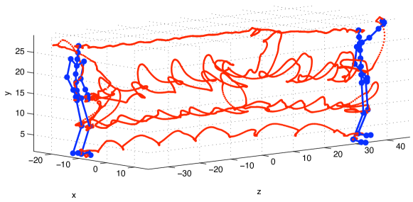
Figure 7.1: With his pioneering light-dot displays, Johansson [90] showed that a great deal of “information” is encoded in the temporal evolution of visual signals. For instance, by the motion of a collection of points positioned at the joints, one can easily infer the type of action, the age group of the actor, his or her mood, etc. despite the fact that all pictorial cues have been eliminated from the image.

As we have discussed in the previous chapter, templates average the data with respect to the distribution of the nuisances, regardless of temporal ordering. Temporal continuity provides a mechanism for tracking, as discussed in Section 5.1, but is otherwise irrelevant for the purpose of describing static scenes or rigid objects. Temporal averaging in the template is, in general, suboptimal, so one could consider statistics other than the average, for instance the entire temporal distribution, as we have done in Section 6.4. While that approach improves the descriptor in the sense of retaining the distributional properties, it still does not respect temporal ordering. These are just two approaches to canonizing time by either averaging or binning. Other approaches include a variety of “spatio-temporal interest point detectors” [194, 104] or other aggregated spatio-temporal statistics [45].

If we are interested in visual decisions involving classes of “objects” that have a temporal component, then all approaches that “canonize” time necessarily mod-out also the temporal variation of interest, in the same way in which canonizing viewpoint eliminates the dependency of the invariant descriptor on the shape of the scene (Section 6.2). At the opposite end of the spectrum one could retain the entire time series (the temporal evolution of feature descriptors) (6.1), and compare them as functions of time using any functional norm in the calculation of the classifier (Section 2.1). This would not yield a viable result because the same action, performed slower or faster, or observed from a different initial time, would result in completely different time series (6.1), if not properly managed. Proper management here means that time should not just be canonized (as in a template or Time HOG) or ignored (by comparing time series as functions), but instead should be marginalized or max-outed. The only difference between these approaches is the prior on time, which is typically either uniform or exponentially decaying, so we will focus on a uniform prior, corresponding to a max-out process for time.

The simplest mechanism to max-out time is known as dynamic time warping (DTW). Dynamic time warping consists in a reparametrization of the temporal axis, via a function $\tau\leftarrow h(t)$, that is continuous and monotonic (in other words, a contrast transformation as defined it in Section 2.2). Accordingly, the dynamic time warping distance is the distance obtained by max-outing the time warping between two time series. The problem with DTW is that it preserves temporal ordering but little else. The moment one alters the time variable, all the velocities (and therefore accelerations, and therefore forces that generated the motion) are changed, and therefore the outcome of DTW does not preserve any of the dynamic characteristics of the original process that generated the data. In other words, if the time series was generated by a dynamical model, DTW does not respect the constraints imposed by the dynamics. This means that a large number of different “actions” are lumped together under DTW. The pioneering work of the psychologist Johansson, however, showed that a great deal of information can be encoded in the temporal signal (Figure 7.1). This information is destroyed by DTW.

The next two sections describe DTW and point the way to generalizing it to take into account dynamic constraints. The reader who is uninterested in the subtleties of recognizing events or actions that have similar appearance but different temporal signatures can skip the rest of this chapter.

7.1 Dynamic time warping revisited

If we consider two time series of images, $I_{1}$ and $I_{2}$, where $I_{j}\doteq\{I_{j}(t)\}_{t=1}^{T}$, for simplicity assumed to have the same length, then the simplest distance we could define is the ${L}^{2}$ norm of the difference, $d_{0}(I_{1},I_{2})=\int_{0}^{T}\|I_{1}(t)-I_{2}(t)\|^{2}dt$, which corresponds to a generative model where both sequences come from an (unknown) underlying process $\{h(t)\}$, corrupted by two different realizations of additive white zero-mean Gaussian “noise” (here the word noise lumps all unmodeled phenomena, not necessarily associated to sensor errors)

$$I_{j}(t)=h(t)+n_{j}(t)~{}~{}~{}j=1,2;\ t\in[0,\ T]$$ (7.1)

The ${L}^{2}$ distance is then the (maximum-likelihood) solution for $h$ that minimizes

$$d_{0}(I_{1},I_{2})=\min_{h}\phi_{data}(I_{1},I_{2}|h)\doteq\sum_{j=1}^{2}\int_{0}^{T}\|n_{j}(t)\|^{2}dt$$ (7.2)

subject to (7.1). Here $h$ can be interpreted as the average of the two time series, and although in principle $h$ lives in an infinite-dimensional space, no regularization is necessary at this stage, because the above has a trivial closed-form solution. However, later we will need to introduce regularizers, for instance of the form $\phi_{reg}(h)=\int_{0}^{T}\|\nabla h\|dt$. This admittedly unusual way of writing the ${L}^{2}$ distance makes the extension to more general models simpler, as we discuss in the next sections.

Consider now an arbitrary contrast transformation $m$ of the interval $[0,T]$, called a time warping, so that (7.1) becomes

$$I_{j}(t)=h(m_{j}(t))+n_{j}(t)~{}~{}~{}j=1,2.$$ (7.3)

The data term of the cost functional we wish to optimize is still $\sum_{i=1}^{2}\int_{0}^{T}\|n_{j}(t)\|^{2}dt$, but now subject to (7.3), so that minimization is with respect to the unknown functions $m_{1}$ and $m_{2}$ as well as $h$. Since the model is under-determined, we must impose regularization [97] to compute the time-warping distance

$$d_{1}(I_{1},I_{2})=\min_{h\in{\bf H},m_{j}\in{\cal M}}\phi_{data}(I_{1},I_{2}|h,m_{1},m_{2})+\phi_{reg}(h).$$ (7.4)

Here $\bf H$ is a suitable space where $h$ is assumed to live and $\cal M$ is the space of monotonic continuous (contrast) transformations. In order for $\tau\doteq m(t)$ to be a viable temporal index, $m$ must satisfy a number of properties. The first is continuity (time, alas, does not jump); in fact, it is common to assume a certain degree of smoothness, and for the sake of simplicity we will assume that $m_{i}$ is infinitely differentiable. The second is causality: The ordering of time instants has to be preserved by the time warping, which can be formalized by imposing that $m_{i}$ be monotonic. We can re-write the distance above as

$$\min_{h\in{\bf H},m_{i}\in{\cal U}}\sum_{j=1}^{2}\int_{0}^{T}\|I_{j}(t)-h(m_{j}(t))\|^{2}+\lambda\|\nabla h(t)\|dt$$ (7.5)

where $\lambda$ is a tuning parameter that can be set equal to zero, for instance by choosing $h(t)=I_{1}(m_{1}^{-1}(t))$, and the assumptions on the warpings $m_{i}$ are implicit in the definition of the set $\cal M$. This is an optimal control problem, that is solved globally using dynamic programming in a procedure called “dynamic time warping” (DTW).

It is important to note that there is nothing “dynamic” about dynamic time warping, other than its name. There is no requirement that the warping function $x$ be subject to dynamic constraints, such as those arising from forces, inertia etc. However, some notion of dynamics can be coerced into the formulation by characterizing the set $\cal M$ in terms of the solution of a differential equation. Following [147], as shown by [121], one can represent allowable $x\in{\cal M}$ in terms of a small, but otherwise unconstrained, scalar function $u$: ${\cal M}=\{m\in{H}^{2}([0,\ T])\ |\ddot{x}=u\dot{x};\ u\in{L}^{2}([0,T])\}$ where ${H}^{2}$ denotes a Sobolev space. If we define $s_{i}\doteq\dot{m}_{i}$ then $\dot{s}=us$; we can then stack the two into $g\doteq[m,\ s]^{T}$, indicative of a group (invertible nuisance) and $C=[1,\ 0]$, and write the data generation model as

$$\begin{cases}\dot{g}_{j}(t)=f(g_{j}(t))+l(g_{j}(t))u_{i}(t)\\ I_{j}(t)=h(Cg_{j}(t))+n_{i}(t)\end{cases}$$ (7.6)

as done by [121], where $u_{i}\in{L}^{2}([0,T])$. Here $f,l$ and $C$ are given, and $h,m_{j}(0),u_{i}$ are nuisance parameters that are eliminated by minimization of the same old data term $\sum_{j=1}^{2}\int_{0}^{T}\|n_{j}(t)\|^{2}dt$, now subject to (7.6), with the addition of a regularizer $\lambda\phi_{reg}(h)$ and an energy cost for $u_{i}$, for instance $\phi_{energy}(u_{i})\doteq\int_{0}^{T}\|u_{i}\|^{2}dt$. Writing explicitly all the terms, the problem of dynamic time warping can be written as

$$d_{3}(I_{1},I_{2})=\min_{h,u_{j},m_{j}}\sum_{j=1}^{2}\int_{0}^{T}\|I_{i}(t)-h(Cg_{j}(t))\|+\lambda\|\nabla h(t)\|+\mu\|u_{i}(t)\|dt$$ (7.7)

subject to $\dot{g}_{j}=f(g_{i})+l(g_{j})u_{i}$. Note, however, that this differential equation is only an expedient to (softly) enforce causality by imposing a small “time curvature” $u_{i}$.

7.2 Time warping under dynamic constraints

The strategy to enforce dynamic constraints in dynamic time warping is illustrated in Figure 7.2:

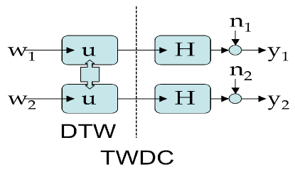
Figure 7.2: Traditional dynamic time warping (DTW) assumes that the data come from a common function that is warped in different ways to yield different time series. In time warping under dynamic constraints (TWDC), the assumption is that the data are the output of a dynamic model, whose inputs are warped versions of a common input function.

Rather than the data being warped versions of some common function, as in (7.3), we assume that the data are outputs of dynamical models driven by inputs that are warped versions of some common function. In other words, given two time series $\{I_{i}\},i=1,2$, we will assume that there exist suitable matrices $A,B,C$, state functions $m_{i}$ of suitable dimensions, with their initial conditions, and a common input $u$ such that the data are generated by the following model, for some warping functions $w_{i}\in{\cal M}$:

$$\begin{cases}\dot{m}_{j}(t)=Am_{j}(t)+Bu(w_{j}(t))\\ I_{j}(t)=Cm_{j}(t)+n_{j}(t).\end{cases}$$ (7.8)

Our goal is to find the distance between the time series by minimizing with respect to the nuisance parameters the usual data discrepancy $\sum_{j=1}^{2}\int_{0}^{T}\|n_{j}(t)\|^{2}dt$ subject to (7.8), together with regularizing terms $\bar{\phi}_{reg}(u)$ and with $w_{j}\in{\cal M}$. Notice that this model is considerably different from the one discussed in the previous section, as the state $g$ earlier was used to model the temporal warping, whereas now it is used to model the data, and the warping occurs at the level of the input. It is also easy to see that the model (7.8), despite being linear in the state, includes (7.6) as a special case, because we can still model the warping functions $w_{i}$ using the differential equation in (7.6). In order to write this time warping under dynamic constraint problem more explicitly, we will use the following notation:

$$I(t)=Ce^{At}I(0)+\int_{0}^{t}Ce^{A(t-\tau)}Bu(w(\tau))d\tau\doteq L_{0}(x(0))+L_{t}(u(w))$$ (7.9)

in particular, notice that $L_{t}$ is a convolution operator, $L_{t}(u)=F*u$ where $F$ is the transfer function. We first address the problem where $A,B,C$ (and therefore $L_{t}$) are given. For simplicity we will neglect the initial condition, although it is easy to take it into account if so desired. In this case, we define the distance between the two time series

$$d_{4}(I_{1},I_{2})=\min\sum_{j=1}^{2}\int_{0}^{T}\|I_{j}(t)-L_{t}(u_{j}(t))\|+\lambda\|u_{j}(t)-u_{0}(w_{j}(t))\|dt$$ (7.10)

subject to $u_{0}\in{\bf H}$ and $w_{j}\in{\cal M}$. Note that we have introduced an auxiliary variable $u_{0}$, which implies a possible discrepancy between the actual input and the warped version of the common template. This problem can be solved in two steps: A deconvolution, where $u_{i}$ are chosen to minimize the first term, and a standard dynamic time warping, where $w_{i}$ and $u_{0}$ are chosen to minimize the second term. Naturally the two can be solved simultaneously.

When the model parameters $A,B,C$ are common to the two models, but otherwise unknown, minimization of the first term corresponds to blind system identification, which in general is ill-posed barring some assumption on the class of inputs $u_{i}$. These can be imposed in the form of generic regularizers, as common in the literature of blind deconvolution [64], or by restricting the classes of inputs to a suitable class, for instance sparse “spikes” [149]. This is a general and broad problem, beyond our scope here, so we will forgo it in favor of an approach where the input is treated as the output of an auxiliary dynamical model, also known as exo-system [81]. This combines standard DTW, where the monotonicity constraint is expressed in terms of a double integrator, with TWDC, where the actual stationary component of the temporal dynamics is estimated as part of the inference. The generic warping $w$, the output of the exo-system satisfies

$$\begin{cases}\dot{w}_{j}(t)=g_{j}(t),~{}~{}~{}j=1,2\\ \dot{g}_{j}(t)=v_{j}(t)g_{j}(t)\end{cases}$$ (7.11)

and $w_{j}(0)=0,\ w_{j}(T)=T$. This is a multiplicative double integrator; one could conceivably add layers of random walks, by representing $v_{i}$ as Brownian motion. Combining this with the time-invariant component of the realization yields the generative model for the time series $I_{i}$:

$$\begin{cases}\dot{w}_{j}(t)=g_{j}(t),~{}~{}~{}i=1,2\\ \dot{g}_{j}(t)=v_{i}(t)g_{j}(t)\\ \dot{m}_{j}(t)=Am_{j}(t)+Bu(w_{j}(t))\\ I_{j}(t)=Cm_{j}(t)+n_{j}(t).\end{cases}$$ (7.12)

Note that the actual input function $u$, as well as the model parameters $A,B,C$, are common to the two time series. A slightly relaxed model, following the previous subsection, consists of defining $u_{i}(t)\doteq u(w_{i}(t))$, and allowing some slack between the two; correspondingly, to compute the distance one would have to minimize the data term

$$\phi_{data}(I_{1},I_{2}|u,w_{i},A,B,C)\doteq\sum_{j=1}^{2}\int_{0}^{T}\|n_{j}(t)\|^{2}dt$$ (7.13)

subject to (7.12), in addition to the regularizers

$$\bar{\phi}_{reg}(v_{i},u)=\sum_{i=1}^{2}\int_{0}^{T}\|v_{i}(t)\|^{2}+\|\nabla u(t)\|^{2}dt$$ (7.14)

which yields a combined optimization problem

$$d_{5}(I_{1},I_{2})=\min_{u,v_{j}\in{L}^{2},A,B,C}\sum_{j=1}^{2}\int_{0}^{T}(\|I_{j}(t)-Cm_{j}(t)\|^{2}+\|v_{j}(t)\|^{2}+\|\nabla u(t)\|^{2})dt$$ (7.15)

subject to (7.12). This distance can be either computed in a globally optimal fashion on a discretized time domain using dynamic programming, or we can run a gradient descent algorithm based on the first-order optimality conditions. The bottom line is that one could use any of the distances introduced in this section, $d_{0},\dots,d_{5}$, to compare time series, corresponding to different forms of marginalization or max-out.

This concludes the treatment of descriptors. The next chapters focus on how to construct a representation from data, and how to aggregate different objects under the same category as part of the learning process.

Chapter 8 Visual exploration

In this chapter we study the inverse problem of hallucination, introduced in Section 3.1, that is the problem of exploration. Whereas hallucination produces images given a representation; exploration produces a representation given images. The goal of exploration is to actively control the data acquisition process in such a way that aggregating Actionable Information eventually yields a complete representation. As we acquire more and more data, the hope is that the set of representations that are compatible with the data shrinks, although not necessarily to a singleton (a complete representation is not necessarily unique). In other words, we hope that the exploration process will reduce the uncertainty on the representation. When and if the inferred representation is complete, it can synthesize the light-field of the original scene up to the uncertainty of the sensors, and we say we have performed sufficient exploration. Exploration can be more or less efficient, in the sense that sufficiency can be achieved with a varying cost of resources (e.g. time, energy).

Exploration is the process that links maximal invariants, $\phi^{\wedge}(I)$, whose complexity we called Actionable Information (AI), to minimal sufficient statistics of a complete representation, whose complexity we called complete information (CI). Because of non-invertible nuisances, the gap between AI and CI can be filled by exercising some form of control on the sensing process. Such control could be exercised in data space, for instance by choosing the most informative features, or in sensor space, for instance by selecting sensing assets in a sensor network, or in physical space, for instance by moving around an occlusion or moving closer to an unresolved region of the scene.

We start by designing a myopic explorer, driven simply by the maximization of Actionable Information. Ideally, by accumulating AI, one would hope to converge to the CI. Unfortunately, this is in general not the case for such a myopic explorer. We therefore consider a slightly less primitive explorer seeking to maximize its reward over a receding horizon. Again, in general, this strategy is not guaranteed to achieve complete efficient exploration. Thus, the modeling exercise points to the need to endow the explorer with memory that can summarize in finite complexity the results of past explorations. Such a memory will be precisely the representation we are after, and we discuss inference criteria that can drive the building of a representation. In some simple instances, such criteria yield viable computational procedures.

In all cases, occlusions and scaling/quantization play a critical role in exploration, a process that can be thought of as the inversion of such nuisances. Therefore, at the outset, we will need efficient methods to perform occlusion detection, to be used either instantaneously – by comparing two temporally adjacent images, as in myopic memoryless exploration – or incrementally, by comparing each new image with the one hallucinated from the current representation.

8.1 Occlusion detection

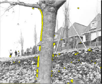
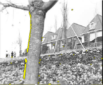
Figure 8.1: Motion estimates for the Flower Garden sequence (left), residual $e$ (center), and occluded region (right) (courtesy of [8]).

In this section we summarize the results of [8], where it is shown that occlusion detection can be formulated as a variational optimization problem and relaxed to a convex optimization, that yields a globally optimal solution. We do not delve on the implementation of the solution, for which the reader is referred to [8], but we describe the formalization of the problem. The reader uninterested in the specifics can skip the rest of this section and assume that the region $\Omega(t)\subset D\subset\mathbb{R}^{2}$ that is not co-visible in two adjacent images has been inferred. Note that this region is not necessarily simply connected or regular, as Figure 8.2 illustrates.

Remark 11 (Optical flow and motion field)

Optical flow refers to the deformation of the domain of an image that results from ego- or scene motion. It is, in general, different from the motion field, (2.9), that is the projection onto the image plane of the spatial velocity of the scene [189], unless three conditions are satisfied: Lambertian reflection, constant illumination, and co-visibility. We have already adopted the Lambertian assumption in Section 2.2, and it is true that most surfaces with benign reflectance properties (diffuse/specular) can be approximated as Lambertian almost everywhere under diffuse or sparse illuminants (e.g. the sun). In any case, widespread violation of Lambertian reflection does not enable correspondence [164], so we will embrace it like the majority of existing approaches to motion estimation. Similarly, constant illumination is a reasonable assumption for ego-motion (the scene is not moving relative to the light source), and even for objects moving (slowly) relative to the light source. Co-visibility is the third and crucial assumption that has to do with occlusions and until recently has been widely neglected in the computation of optical flow. If an image contains portions of its domain that are not visible in another image, these can patently not be mapped onto it by optical flow vectors. Constant visibility is often assumed because optical flow is defined in the limit where two images are sampled infinitesimally close in time, in which case there are no occluded regions, and one can focus solely on discontinuities of the motion field. But the problem is not that optical flow is discontinuous in the occluded regions; it is simply not defined; it does not exist. By definition, an occluded region cannot be explained by a displaced portion of a different image, since it is not visible in the latter. Motion in occluded regions can be hallucinated (extrapolated, or “inpainted”) but not validated on data.

Remark 12 (The Aperture problem)

The aperture problem refers to the fact that the motion field at a point can only be determined in the direction of the gradient of the image at that point (Figure 3.7). Therefore, occlusions can only be determined if the gradient of the radiance intersects transversally the boundary of the occluded region. When this does not happen (for instance when a region with constant radiance occludes another one with constant radiance), an occlusion cannot be positively discerned from a material boundary or an illumination boundary. For instance, in the Flower Garden sequence (Figure 8.1), the (uniform) sky could be attached to the branches of the tree, or it could be occluded by them. Often, priors or regularizers are imposed to resolve this ambiguity, but again such a choice is not validated from the data. We prefer to maintain the ambiguities in the representation, deferring the decision to the exploration process, when data becomes available to disambiguate the solution (e.g. the tree passing in front of a cloud). This naturally occurs over time as the initial representation converges towards the complete representation.

For clarity, we denote a time-varying image via $I:D\subset\mathbb{R}^{2}\times\mathbb{R}^{+}\rightarrow\mathbb{R}^{+};\ (x,t)\mapsto I(x,t)$. Under the Lambertian assumption, as we have seen in Section 5.1, the relation between two consecutive images in a video $\{I(x,t)\}_{t=0}^{T}$ is given by

$$I(x,t+dt)=\begin{cases}I(w(x,t),t)+n(x,t),~{}~{}~{}x\in D\backslash\Omega(t;dt)\\ \nu(x,t),~{}~{}~{}x\in\Omega(t;dt)\end{cases}$$ (8.1)

where $w:D\times\mathbb{R}^{+}\rightarrow\mathbb{R}^{2}$ is the optical flow (2.10) which approximates the motion field (2.9) and is defined everywhere except at occluded regions $\Omega$. These can change over time and depend on the temporal sampling interval $dt$; $\Omega$ is in general not simply-connected, so even if we call $\Omega$ the occluded region (singular), it is understood that it is made of multiple connected components. In the occluded region, the image can take any value $\nu:\Omega\times\mathbb{R}^{+}\rightarrow\mathbb{R}^{+}$ that is in general unrelated to $I(x,t)_{|_{x\in\Omega}}$. Because of (almost-everywhere) continuity of the scene and its motion (i), and because the additive term $n(x,t)$ compounds the effects of a large number of independent phenomena and therefore we can invoke the Law of Large Numbers (ii), in general we have that

$${\rm(i)}~{}~{}\lim_{dt\rightarrow 0}\Omega(t;dt)=\emptyset,~{}~{}~{}{\rm and}~{}~{}~{}{\rm(ii)}~{}~{}n\stackrel{{\scriptstyle IID}}{{\sim}}{\cal N}(0,\lambda)$$ (8.2)

i.e. , the additive uncertainty is normally distributed in space and time with an isotropic and small variance $\lambda>0$. Note that we are using the (overloaded) symbol $\lambda$ for the covariance of the noise, whereas usually we have employed the symbol $\sigma$. The reason for this choice will become clear in Equation (8.17), where $\lambda$ will be interpreted as a Lagrange multiplier. We define the residual

$$e:D\rightarrow\mathbb{R}^{+}{;(x,t)\mapsto e(x,t;dt)\doteq I(x,t+dt)-I(w(x,t),t)}$$

on the entire image domain $x\in D$, via (for simplicity we omit the arguments of the functions when clear from the context)

$$e(x,t;dt)\doteq I(x,t+dt)-I(w(x,t),t)=\begin{cases}n(x,t),~{}~{}~{}x\in D\backslash\Omega{}\\ \nu(x,t)-I(w(x,t),t)~{}~{}~{}~{}x\in\Omega{}\end{cases}$$ (8.3)

which we can write as the sum of two terms, $e_{1}:D\rightarrow\mathbb{R}^{+}$ and $e_{2}:D\rightarrow\mathbb{R}^{+}$, also defined on the entire domain $D$ in such a way that

$$\begin{cases}e_{1}(x,t;dt)=\nu(x,t)-I(w(x,t),t),~{}~{}~{}x\in\Omega{}\\ e_{2}(x,t;dt)=n(x,t),~{}~{}~{}~{}~{}~{}x\in D\backslash\Omega{}.\end{cases}$$ (8.4)

Note that $e_{2}$ is undefined in $\Omega$, and $e_{1}$ is undefined in $D\backslash\Omega$, in the sense that they can take any value there, including zero, which we will assume henceforth. We can then write, for any $x\in D$,

$$I(x,t+dt)=I(w(x,t),t)+e_{1}(x,t;dt)+e_{2}(x,t;dt)$$ (8.5)

and notice that, because of (i), $e_{1}$ is large but sparse, while because of (ii) $e_{2}$ is small but dense. We will use this as an inference criterion for $w$, seeking to optimize a data fidelity criterion that minimizes the $L^{0}$ norm of $e_{1}$ (a proxy of the area of $\Omega$), and the log-likelihood of $n$ (the Mahalanobis norm relative to the variance parameter $\lambda$)

$$\psi_{\rm data}(w,e_{1})\doteq\|e_{1}\|_{{L}^{0}(D)}+\frac{1}{\lambda}\|e_{2}\|_{{L}^{2}(D)}~{}~{}~{}{\rm subject\ to\ }(\ref{eq-mod+})$$ (8.6)

$$=\frac{1}{\lambda}\|I(x,t+dt)-I(w(x,t),t)-e_{1}\|_{{L}^{2}(D)}+\|e_{1}\|_{{L}^{1}(D)}$$

where $\|f\|_{L^{0}(D)}=\int\chi_{f(x)\neq 0}(x)dx$ is relaxed as usual to $\|f\|_{{L}^{1}(D)}\doteq\int_{D}|f(x)|dx$ and $\|f\|_{{L}^{2}(D)}\doteq\int_{D}|f(x)|^{2}dx$. Since we wish to make the cost of an occlusion independent of the brightness of the (un-)occluded region, we can replace the $L^{1}$ norm with a re-weighted $\ell^{1}$ norm that provides a better approximation of the $L^{0}$ norm [9].

Unfortunately, we do not know anything about $e_{1}$ other than the fact that it is sparse, and that what we are looking for is $\chi_{\Omega}\propto e_{1}$, where $\chi:D\rightarrow\mathbb{R}^{+}$ is the characteristic function that is non-zero when $x\in\Omega$, i.e. , where the occlusion residual is non-zero. So, the data fidelity term depends on $w$ but also on the characteristic function of the occlusion domain $e_{1}$. Using the formal (differential) notation for first-order differences (note that this is just a symbolic notation, as we do not let $dt\rightarrow 0$, lest we would have $\Omega\rightarrow\emptyset$)

$$\nabla I(x,t) \doteq \left[\begin{array}[]{c}I\left(x+\left[\begin{array}[]{c}1\\ 0\end{array}\right],t\right)-I(x,t)\\ I\left(x+\left[\begin{array}[]{c}0\\ 1\end{array}\right],t\right)-I(x,t)\end{array}\right]^{T}$$ (8.13)

$$I_{t}(x,t) \doteq I(x,t+dt)-I(x,t)$$ (8.14)

$$v(x,t) \doteq w(x,t)-x$$ (8.15)

we can approximate, for any $x\in D\backslash\Omega$,

$$I(x,t+dt)=I(x,t)+\nabla I(x,t)v(x,t)+n(x,t)$$ (8.16)

where the linearization error has been incorporated into the uncertainty term $n(x,t)$. Therefore, following the same previous steps, we have

$$\boxed{\psi_{\rm data}(v,e_{1})=\int_{D}|\nabla Iv+I_{t}-e_{1}|^{2}dx+\lambda\int_{D}|e_{1}|dx}$$ (8.17)

Since we typically do not know the variance $\lambda$ of the process $n$, we will treat it as a tuning parameter, and because $\psi_{\rm data}$ or $\lambda\psi_{\rm data}$ yield the same minimizer, we have attributed the multiplier $\lambda$ to the second term. In addition to the data term, because the unknown $v$ is infinite-dimensional, we need to impose regularization, for instance by requiring that the total variation (TV) of $v$ be small

$$\psi_{\rm reg}(v)=\mu\int_{D}\|\nabla v\|dx$$ (8.18)

where $\mu$ is a multiplier to weigh the strength of the regularizer. TV is desirable in the context of occlusion detection because it does not excessively penalize motion discontinuities, that can occur where motion is parallel to the occluding boundary (so there is an occluding boundary without an occluded region, for instance where the direction of motion is parallel to the occluding boundary, see Remark 12). The overall problem can then be written as the minimization of the cost functional $\psi=\psi_{\rm data}+\psi_{\rm reg}$, which in a discretized domain (the lattice $D\cap{\mathbb{Z}}^{2}$) becomes

$${\hat{v},\hat{e}_{1}=\arg\min_{v,e}\underbrace{\|\nabla Iv+I_{t}-e\|^{2}_{\ell^{2}}+\lambda\|e\|_{\ell_{rw}^{1}}+\mu\|\nabla v\|_{{\ell}^{1}}}_{\psi(v,e)}}$$ (8.19)

where $\ell^{1}_{rw}$ is the re-weighted $\ell^{1}$ norm [9] and $\ell^{1},\ell^{2}$ are the finite-dimensional version of the functional norms $L^{1}(D),L^{2}(D)$. The remarkable thing about this minimization problem is that $\psi$ is convex in the unknowns $v$ and $e$. Therefore, convergence to a global solution can be guaranteed for an iterative algorithm regardless of initial conditions [27]. This follows immediately after noticing that the ${\ell}^{2}$ term

$$\|\underbrace{[\nabla I,-Id]}_{A}\left[\begin{array}[]{c}v\\ e\end{array}\right]+\underbrace{I_{t}}_{b}\|_{{\ell}^{2}}$$ (8.20)

is linear in both $v$ and $e$, the gradient (first-difference) $\nabla v$ is a linear operator, and the ${\ell}^{1}$ norm is a convex function.

Not only is this result appealing on analytical grounds, but is also enables the deployment of a vast arsenal of efficient optimization schemes, as proposed in [8]. In practice, although the global minimizer does not depend on the initial conditions, it does depend on the multipliers $\lambda$ and $\mu$, for which no “right choice” exists, so an empirical evaluation of the scheme (8.19) is necessary [8].

It is tempting to impose some type of regularization on the occluded region $\Omega$ (for instance that its boundary be “short”), but we have refrained from doing so, for good reasons. In the presence of smooth motions, the occluded region is guaranteed to be small, but under no realistic circumstances is it guaranteed to be simple. For instance, walking in front of a barren tree in the winter, the occluded region is a very complex, multiply-connected, highly irregular region that would be very poorly approximated by some compact regularized blob (Figure 8.2).

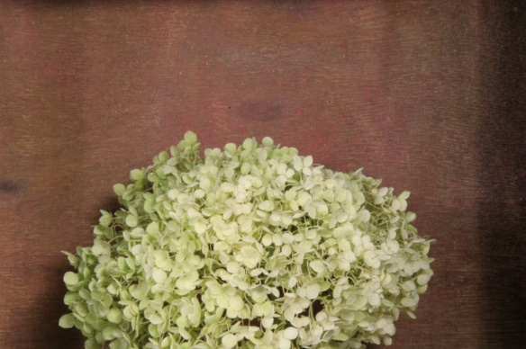
Figure 8.2: Occlusion regions for natural scenes (left) can have rather complex structure (middle) that would be destroyed if one were to use generic regularizers for the occluded region $\Omega$. The disparity maps (right) should only be evaluated in the co-visible regions (black regions in the middle figure), since disparity cannot be ascertained in the occluded region.

Source code to perform simultaneous motion estimation and occlusion detection is available on-line from [8]. It can be used as a seed to detect detached objects, or better detachable objects [11], or to temporally integrate occlusion information so as to infer depth layers as done in [84, 83]. We will, however, defer the temporal integration of occlusion information to the next sections, where we discuss the exploration process. For now, what matters is that it is possible, given either two adjacent images, $I_{t},I_{t+1}$, or an image predicted via hallucination, for instance $\hat{I}_{t+1}$ and a real image $I_{t+1}$, to determine both the deformation taking one image onto the other in the co-visible region, and the characteristic function of such a region, that is the occluded domain.

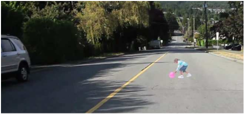
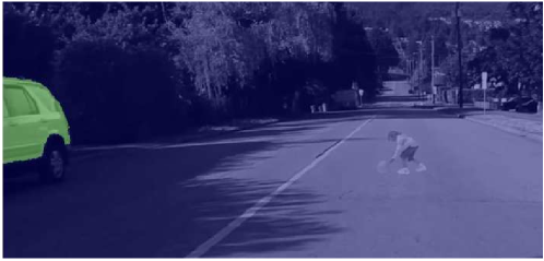
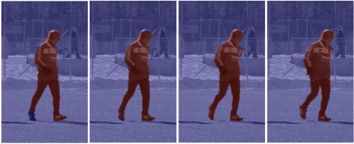
Figure 8.3: Detachable object detection (courtesy of [11]). The “girl” in Figure 1.2 and the soccer player would be similarly classified as bona-fide “objects” by a passive classification/detection/segmentation scheme. However, an extended temporal observation during either ego-motion (top) or object motion (bottom) correctly classifies the car on top and the soccer player on the bottom as “detached objects” but not the girl painted on the road pavement (middle).

In the next section we begin discussing the implication of occlusion detection for exploration.

8.2 Myopic exploration

Consider an image $I_{t}$, taken at time $t$, and imagine using it to predict the next image, $I_{t+1}$. In the next section we describe this process in the absence of non-invertible nuisances. We show that in this case one image is sufficient to determine a complete representation, and there is no need for exploration at all. The story is, of course, different when there are invertible nuisances.

8.2.1 In the absence of non-invertible nuisances

In the absence of occlusions (for instance, if the images are taken by an omni-directional camera inside an empty room) and quantization errors or noise (if the images are samples of the scene radiance that satisfy Nyquist’s condition – if that was possible, that is), and if the scene obeys the Lambert-Ambient-Static model (2.6), the new image can be generated by the old image via a suitable contrast transformation of its range and diffeomorphic deformation of its domain. In other words, the first image $I_{t}$ can be used to construct a representation as we have discussed in Section 2.4.4, which in turn can be used to hallucinate any other image of the same scene, for instance $I_{t+1}$. In fact, from (2.6), we can solve for $\rho$ in the first image via $\rho(p(x))=I_{t}(x)$, where $p(x)=\bar{x}/\|\bar{x}\|$ and substitute in the second, so we have

$$I_{t+1}(w(x))=k\circ I_{t}(x)$$ (8.21)

where $w(x)=\pi g\pi^{-1}(\bar{x}/\|\bar{x}\|)$ and where we have aggregated the two contrast transformations $k_{t+dt}$ and $k_{t}$ into one. This is exactly the hallucination process described in Section 3.1, whereby a single image $I_{t}$, supported on a plane, is interpreted as a representation and used to hallucinate the next image $I_{t+1}$.

In the absence of non-invertible nuisances, the only purpose of the second image is to enable the estimation of the domain deformation $w$ and the contrast transformation $k$ through equation (8.21) [87]. So, the first image captures the radiance $\rho$, and in combination with the second image they capture the shape $S$, entangled with the nuisance $g$ in the domain deformation $w$, as discussed in Section 6.2 and further elaborated in B.3. Any additional image $I_{\tau}$, not necessarily taken at an adjacent time instant, can be explained by these two images. In fact, any additional image can be used to test the hypothesis that it is generated by the same scene, by performing the same exercise with either of the two (training) images, to test whether they are compatible with (i.e. can be generated by) the same scene, except for the residual error $n$ that is temporally and spatially white, and isotropic (homoscedastic). This test consists of an extremization procedure (Section 2.3 and Figure 2.5), whereby nuisance factors, as well as the scene, are inferred as part of the decision process, and the residual has high probability under the noise model. This can be thought of as a “recognition by (implicit) reconstruction” process, and was common in the early days of visual recognition via template matching.

Notice that, as discussed in Section 6.2, contrast (a nuisance) interacts with the radiance, so one can only determine the radiance up to a contrast transformation. Similarly, motion (a nuisance) interacts with the shape/deformation, so one can only determine shape up to a diffeomorphism. If one were to canonize both contrast and domain diffeomorphisms, then some discriminative power would be lost as any two scenes that are equivalent (modulo a domain diffeomorphism, whether or not they are generated by a scene with the same shape) would be indistinguishable from a maximal invariant feature (or from any invariant feature for that matter) [186].

In summary, in the absence of non-invertible nuisances, a single (omni-directional, infinite-resolution, noise-free) image can be used to construct a representation from which the entire light field of the scene can be hallucinated. This is what we called a complete representation. Its minimal sufficient statistic is the Complete Information, and there is no need for exploration. The need for exploration does, of course, arise as soon as non-invertible nuisances are present. The case discussed above is a wild idealization since, even in the absence of occlusions, quantization and noise introduce uncertainty in the process, and therefore there is always a benefit from acquiring additional data, even in the absence of any active control.

8.2.2 Dealing with non-invertible nuisances

In general, equation (8.21) is valid only in the co-visible domain (Section 2.2). Neglecting contrast transformations for simplicity, we have that

$$I_{t+1}(w(x))=I_{t}(x),~{}~{}~{}x\in D\cap w^{-1}(w(D))\subset D.$$ (8.22)

The complement of the co-visible domain is the occluded domain

$$\Omega\doteq D\backslash w^{-1}(w(D))\subset D.$$ (8.23)

Since we will assume that there is a temporal ordering (causality), we will consider only forward occlusions (sometimes called “un-occlusion” or “discovery”); that is, portions of the domain of $I_{t+1}$, $\Omega\subset D$, whose pre-image $w^{-1}(\Omega)$ was not visible in $I_{t}$. The restriction of the image to this subset, $\{I_{t+1}(x),\ x\in\Omega\}$ cannot be explained using $I_{t}$.

Consider now an image $I_{t}$, and imagine using it to predict the next image $I_{t+1}$, as we have done in the previous section. No matter how we choose $w$, we cannot predict exactly what the new image is going to look like in the occluded domain $\Omega$, even if we had an omni-directional, infinite-resolution, noise-free camera. Therefore, in the occluded domain we have a distribution of possible “next images,” based on the priors. The entropy of this distribution measures the uncertainty in the next image, and therefore the potential “information gain” from measuring it (before we actually measure it). Once we discount other nuisance factors, by considering a maximal invariant of the next image in the occluded domain, we have the innovation

$$\epsilon(I,t+1)\doteq\phi^{\wedge}({I_{t+1}}_{|_{\Omega}})$$ (8.24)

whose complexity represents the Actionable Information Increment (AIN):

$$AIN(I,t)\doteq H(\epsilon(I,t+1))={\cal H}({I_{t+1}}_{|_{\Omega}}).$$ (8.25)

The AIN is the uncertainty in the innovation, or the “degree of unpredictability” of future data. The above is the contribution to the AIN due to occlusions, that can be determined as in Section 8.1. However, we also have uncertainty due to quantization and noise. This is simpler to model, as it is usually independent of the scene: Uncertainty due to scaling and quantization increases linearly with distance, and uncertainty due to noise is independent of both the scene and the viewer. In all cases, however, there exists a control action that can reduce uncertainty. For the case of scale, it is zooming, or translating along the optical axis, or increasing the sensor’s resolution. For the case of noise, it is taking repeated (registered) measurements.

In all cases, what yields a non-zero innovation is the presence of non-invertible nuisances, $\nu_{t}$, that include occlusion, quantization, and other unmodeled uncertainty (noise). We then have that the AIN can be computed as the conditional entropy of

$$p(\phi^{\wedge}(I_{t+1})|I_{t})=\int p(\phi^{\wedge}(I_{t+1})|I_{t},\nu_{t})dP(\nu_{t})$$ (8.26)

where we have marginalized over all non-invertible nuisances. We therefore have, for the specific case of just two images,

$$AIN(I,t)\doteq{\cal H}({I_{t+1}}|I_{t}).$$ (8.27)

This construction can be extended to the case where we have measured multiple images up to time $t$, as we discuss in the next section.

Remark 13 (Background subtraction)

The innovation can be thought of as a form of generalized background subtraction. In the most trivial case, the representation is derived from one image only (the background image) and the only motion in the image is due to a “foreground object.” Other background subtraction schemes, including those based on multiple layers or on an aggregate model of the background [98], can be understood in the framework of occlusion detection and innovation under different prediction models [84, 83].

8.2.3 Enter the control

Clearly, the $AIN$ depends on the motion between $t$ and $t+dt$, as well as on the (unknown) scene $\xi$. For a sufficiently small $dt$, $g_{t+dt}=\exp{(\widehat{u}dt)}g_{t}$, where $u\in{\mathfrak{se}}(3)$ is the rigid body velocity of the viewer [117] (assumed constant between $t$ and $t+dt$), the operator $\widehat{~{}~{}}$ is the “hat” operator that maps a $6$-dimensional vector of rotational and translational velocities into a “twist” [117] and ${\mathfrak{se}}(3)$ denotes the Lie algebra of “twists” associated with $SE(3)$ [117]. Thus, the motion between $t$ and $t+dt$ is given by $g_{t+dt}g^{-1}_{t}\simeq Id+\widehat{u}dt$, which one can control by moving the sensor with a velocity $u$. By assuming velocity to be sufficiently small, we can take $dt$ to be the unit time interval, $dt=1$. Therefore, the $AIN$ can, to a certain extent, be controlled. When emphasizing the dependency on the control input, we write $AIN(I,t;u)\doteq{\cal H}(I_{t+1}|I_{t},u_{t})$. A myopic controller would simply try, at each instant, to perform a control action (e.g. a rigid motion, zooming, or capturing and averaging multiple images) so as to maximize the $AIN$:

$$\hat{u}_{t}=\arg\max_{u}AIN(I,t;u).$$ (8.28)

Note that the AIN is computed before the control $u_{t}$ is applied, and therefore before the “next image” $I_{t+1}$ is computed. Thus the AIN involves a distribution of next images, marginalized with respect to all non-invertible nuisances. Once we actually measure the next image, we sample an instance of the innovation process. If we have discovered nothing in the next image, the sample of the innovation will be zero.

Therefore, a myopic agent could easily be stuck in a situation where none of the allowable control actions $u_{t}\in{\cal U}$ yield any information gain. The observer would then stop despite having failed to attain the Complete Information. The observer could also be trapped in a loop where it keeps discovering portions of the scene it has seen before, albeit not in the immediate past, for instance as it moves around a column. This is because the controller (8.28) does not have memory.

To endow the controller with memory we can simply consider the innovation relative to the history $I^{t}\doteq I_{0}^{t}\doteq\{I_{\tau}\}_{\tau=0}^{t}$, rather than relative to just the current image $I_{t}$.

$$\hat{u}_{t}=\arg\max_{u}{\cal H}(I_{t+1}|I^{t},u)$$ (8.29)

There are two problems with this approach: One is that it is still myopic. The other is that the history $I^{t}$ grows unbounded.

8.2.4 Receding-horizon explorer

A slight improvement can be had by planning a controller that maximizes the AIN over a finite horizon, for instance of length $T>1$:

$$\hat{u}_{t}=\arg\max_{u}{\cal H}(I^{t+T}_{t+1}|I^{t},u).$$ (8.30)

Of course, as soon as the agent makes one step, and acquires $I_{t+1}$, the history changes to $I^{t+1}$; therefore, the agent can use the control planned for the $T$-long interval to perform the first step, and then re-plan the control for the new horizon from $t+1$ to $t+T+1$. One can also consider an infinite horizon $T=\infty$, which presents obvious computational challenges. Regardless of the horizon, however, all controllers above have to cope with the fact that the history keeps growing. Even setting aside the fact that no provable guarantees of sufficient exploration exist for this strategy, it is clear that the agent needs to have a finite-complexity memory that summarizes all prior history.

8.2.5 Memory and representation

A memory is a function of past data, $\phi(I^{t})$. Of all functions, we are interested in those that are parsimonious (minimal), and “informative” in the sense that they can generate copies not of the data, but of the maximal invariants of the data. These are the characteristics of what we have defined as a representation. At any given time $t$, we can infer a representation $\hat{\xi}_{t}$ that is compatible with the history $I^{t}$ and that, eventually, may converge to a complete representation $\hat{\xi}$. Building such a representation (memory) is an inference problem that can be framed in the context of exploration as a System Identification problem under a suitable prediction-error criterion [112]. Given a collection of data $I^{t}$, we are interested in determining a “model” $\phi$ such that the statistic $\phi(I^{t})$ best summarizes the entire past $I^{t}$ for the purpose of predicting the entire future $I_{t+1}^{\infty}$. In Remark 14 we will shows that this is equivalent to determining

$$\hat{\xi}_{t}=\arg\min_{\xi}H(\xi|I^{t})\ {\rm subject\ to}\ I^{t}\in{\cal L}(\hat{\xi}_{t}).$$ (8.31)

In prediction-error methods, usually the complexity constraint is enforced by choosing the bound on the order of the model (the number of free parameters), and the entropy is approximated with its empirical estimate, assuming stationarity. For the case where all the densities at play are Gaussian, minimizing the entropy above reduces to minimizing the sum of squared one-step prediction errors. This problem has also been addressed in the literature of information-based filtering [129], but can only be realistically solved for low-dimensional state-spaces [152] using particle filtering, or for linear-Gaussian models (although see [73]).

Note that the condition $I^{t}\in{\cal L}(\hat{\xi}_{t})$ is to be understood up to the noise in the measurement device $n_{t}$, according to (2.18), in the sense that the residual $I_{t}-h(g,\hat{\xi}_{t},\nu)$ has high probability under the noise model $p_{n}$ for all times $t$. Such a “noise” lumps the residual due to all unmodeled phenomena and can be model as spatially and temporally white, and isotropic (homoscedastic). If not, the spatial or temporal structure can be included as part of the representation, until the residual is indeed white. The above equation can then be interpreted as a reduction of uncertainty, specified by the mutual information ${\mathbb{I}}(\xi;I^{t})$, as we have anticipated in Section 2.5.

In a causal exploration process, where data is gathered incrementally, we would like to update the estimate of the representation; by minimizing the conditional entropy above. At the same time, we would like to control the exploration process so as to maximize the AIN. This is discussed in the next section where we describe dynamic explorers.

8.3 Dynamic explorers

In this section we consider an entity including a sensor (a video camera) capable of exercising a control, for instance by changing the vantage point or the characteristics of the sensor (zooming). We call such an entity an explorer. In the absence of any restriction on the control, so long as there are non-invertible nuisances, the $AIN$ provides guidance to perform exploration, and memory provides a way to incrementally build a representation $\hat{\xi}$. Ideally, such a representation would eventually converge to a minimal sufficient statistic of the light field, ${\cal L}(\xi)$, thus accomplishing sufficient exploration. Sufficient exploration, if possible, would enable the absence of evidence to be taken as evidence of absence [145].

We start with one image, say $I_{0}$, and its maximal invariant $\phi^{\wedge}(I_{0})$, that is compatible with a (typically infinite) number of scenes, $\hat{\xi}_{0}$, that are distributed according to some prior $p(\hat{\xi}_{0})$ that has high entropy (uncertainty). Compatibility means that the image $I_{0}$ can be synthesized from $\hat{\xi}_{0}$ up to the modeling residual $n$. As we have seen in Section 3.1, we can easily construct a sample scene by choosing $\hat{S}_{0}$ to be a unit sphere, $S_{0}(x)=p(x)=\frac{\bar{x}}{\|\bar{x}\|}$, and choosing $\rho_{0}(p)=I(x)$ where $p=p(x)$ in the entire sphere but for a set of measure zero. Therefore, we call $\hat{\xi}_{0}=\{\rho_{0},S_{0}\}\doteq h^{-1}(I_{0})$. Clearly, if we had only one image, as we did in Section 3.1, we would not need a representation to explain it, and indeed we do not even need a notion of scene. So, in our case, this is just the initialization of the explorer, which corresponds to one of many possible representations that are compatible with the first image (see Figure 3.1).

Given the initial distribution, $p(\hat{\xi}_{0})$ and the next measurement, $I_{1}$, we can compute an innovation $\epsilon_{1}=I_{1}-h(g_{1},\hat{\xi}_{0},\nu_{1})$, that is a stochastic process that depends on the (unknown) nuisances $g_{1},\nu_{1}$ as well as on the distribution of $\hat{\xi}_{0}$. We can then update such a distribution by requiring that it minimizes the uncertainty of the innovation. The uncertainty in the innovation is the same as the uncertainty of the next measurement, and therefore we can simply minimize the conditional entropy of the next datum, once we have marginalized or max-outed the nuisances: $\hat{\xi}_{1}=\arg\min_{p(\hat{\xi})}{\cal H}(I_{1}|\hat{\xi}_{0})$ where $p(I_{1}|\hat{\xi}_{0})=\int{\cal N}(I_{1}-h(g,\hat{\xi}_{0},\nu))dP(g)dP(\nu)$. In practice, carrying around the entire distribution of representations is a tall order, for the space of shape and reflectance functions do not even admit a natural metric, let alone a probabilistic structure that is computable. So, one may be interested in a point-estimate, for instance one of the (multiple) modes of the distribution, the mean, median, or a set of samples. In any case, we indicate this via $\hat{\xi}_{1}=\arg\min_{p(\hat{\xi}_{1})}{\cal H}(I_{1}|\hat{\xi}_{0})$. Now, instead of marginalizing over all (invertible and non-invertible) nuisances, we can canonize the invertible ones, and therefore, correspondingly, minimize the actionable information gap, instead of the conditional entropy of the raw data: At a generic time $t$, assuming we are given $p(\hat{\xi}_{t-1})$, we can perform an update of the representation via

$$\boxed{\hat{\xi}_{t}=\arg\min_{p(\hat{\xi}_{t})}{\cal H}(I_{t}|\hat{\xi}_{t-1})}=\arg\min H\left(\int{\cal N}(\phi^{\wedge}(I_{t})-h(\hat{\xi}_{t-1},\nu);\sigma)dP(\nu)\right)$$ (8.32)

where ${\cal N}(\mu;\sigma)$ denotes a Gaussian density with mean $\mu$ and isotropic standard deviation $\sigma$. To the equation above we must add a complexity cost, for instance $\lambda H(\hat{\xi}_{t-1})$ where $\lambda$ is a positive multiplier.

Now, at time $t$, the updated representation $\hat{\xi}_{t}$ can be used to extrapolate the next image $I_{t+1}$. The hallucination process carries some uncertainty because of the non-invertible nuisances, and this uncertainty is precisely the information gain to come from the next image. Since the next image depends on where we have moved (or, more in general, on what control action we have exercised), we can choose the control $u_{t}$ so that the next image $I_{t+1}$ will be most informative, i.e.

$$\boxed{\hat{u}_{t}=\arg\max_{u\in{\cal U}}{\cal H}(I_{t+1}|\hat{\xi}_{t},u)}=\arg\max H\left(\int{\cal N}(\phi^{\wedge}(I_{t+1})-h(\hat{\xi}_{t},\nu);\sigma)dP(\nu)\right)$$ (8.33)

where $\cal U$ includes complexity or energy costs associated with the control action $u$. Thus, inference and control are working together, one to maximize the uncertainty of the next data, the other to minimize it.

Technically, the most informative next data would be the ones that produce the largest reduction in uncertainty, i.e. $\arg\max{\mathbb{I}}(\xi;I^{t+1})=H(\xi)-H(\xi|I^{t+1})$. Unfortunately, as we have already discussed, even defining a base measure in the space of scenes is difficult, so computing $H(\xi)$ is problematic. However, we can rewrite the mutual information above in terms of the entropy of the data, $H(I_{t+1}|I^{t},u)-H(I_{t+1}|\xi,u).$ Now, given the scene $\xi$, even the non-invertible nuisances $\nu$ become invertible, so $p(I_{t+1}|\xi,u)$ only depends on the residual uncertainty, that comes from all unmodeled phenomena and can realistically be considered white, independent, and isotropic (otherwise, if it has considerable structure, this should be modeled explicitly as a nuisance $\nu$). Therefore, the conditional entropy $H(I_{t+1}|\xi,u)$ is independent of $u$, and we can focus on the first term $H(I_{t+1}|I^{t},u)$, which is what we have done in (8.33) after handling the invertible nuisance via pre-processing with $\phi^{\wedge}$.

The construction of a representation from a collection of data treated as a batch has been described in [84, 83] for the case of multiple occlusion layers portraying arbitrarily deforming objects, and in [87] for the case of rigid objects generating self-occlusions. This requires the dynamic update of the visible portion of the domain as a result of the update of the representation. In the case of [87], the representation consisted of an explicit model of the geometry of the scene (a collection of piecewise smooth surfaces) as well as of the photometry of the scene, consisting of the radiant tensor field, that could be used to generate “super-resolution images” (i.e. images hallucinated at a resolution higher than that of the native sensor that collected the original data), as well as to generate views from different vantage points despite non-Lambertian reflection. In all these cases, the uncertainty was assumed Gaussian, so minimum-entropy estimation reduces to wide-sense filtering (minimum-variance).

The design of a control action, given the current representation, for the case of uncertainty due to visibility has been described in [181, 182] for compact spaces, and extended in [76] for unbounded domains. The case where uncertainty due to scale and noise is also present has been described in [94].

Note that, in general, there is no guarantee that $\hat{\xi}_{t}\rightarrow\xi$ in any meaningful sense. The most we can hope for is that ${\cal L}(\hat{\xi}_{t})\rightarrow{\cal L}(\xi)$, as we have pointed out. In other words, what we can hope is that our representation can at most generate data that is indistinguishable from the real data, up to the characteristics of the sensor. Since the inference of a representation is guided by a control, and the hallucination process requires the simulation of the invertible nuisance $g$ (which includes vantage point), Koenderink’s famous characterization of images as “controlled hallucinations” is particularly fitting. Following the analysis above we can say that the representation $\hat{\xi}$ is obtained through a controlled exploration (perception) process, and from the representation we can then hallucinate images in a controlled fashion.

In general, however, it is not possible to guarantee that the exploration process will converge, even in the sense of (2.18) ${\cal L}(\hat{\xi}_{t})\rightarrow{\cal L}(\xi)$. However, it is trivial to design exhaustive control policies that, under suitably benign assumptions on the environment (that the scene is bounded, that the topology is trivial, and that the radiance obeys some sparsity or band-limited assumption) will achieve sufficient exploration, at least asymptotically:

$$\hat{\xi}_{t}\rightarrow\hat{\xi}~{}~{}~{}~{}~{}{\rm s.\ t.}~{}~{}~{}~{}~{}{\cal L}(\hat{\xi})={\cal L}(\xi).$$ (8.34)

For instance, a Brownian motion restricted to the traversable space will, eventually, achieve complete exploration of a static environment.

The goal of exploration is, therefore, to trade off the efficiency of the exploration process, including the cost of computing an approximation to the policy (8.32)-(8.33), with the probability of achieving sufficient exploration. This is beyond the scope of this manuscript and we refer the reader to the vast literature on Optimal Control, Path Planning, Robotic Exploration, and partially-observable Markov Decision Processes (POMDP) in Artificial Intelligence. For the case of uncertainty due to visibility (occlusions) both [76, 181] provide bounds on the expected path length as a function of the complexity of the environment.

The discussion above suffices to our purpose of closing the circle on the issue of representation introduced in Section 2.4.4 and discussed in Section 3.1, by providing means to approximate it asymptotically from measured data. At any given instant of time, our representation $\hat{\xi}_{t}$ is incomplete, and any discrepancy between the observed images and the images hallucinated by the representation (the innovation) can be used to update the representation and reduce the uncertainty in $\hat{\xi}$.

The fact that, to ensure inference of a complete representation, a control $u$ must be exercised, links the notion of representation (and therefore of information) inextricably to a control action. More precisely, the exploration process links the control to the representation, and actionable information to the complete information. This discussion, of course, only pertains to the limiting case where we have arbitrary control authority to move in free space, into every nook and cranny (to invert occlusions), to zoom-in or move arbitrarily close and have arbitrarily high sampling rate (image resolution, to invert quantization), and to stay arbitrarily long in front of a static scene (or to sample in time arbitrarily fast relative to the time constant of the temporal changes in the scene), to invert noise. The opposite extremum is when we have no control authority whatsoever, in which case all we can compute is a maximal invariant and its actionable information, as discussed in Section 2.5. In this case the Actionable Information Gap cannot be closed.

In between, we can have scenarios whereby a limited control authority can afford us an increase in actionable information by aggregating the $AIN$ over time, thus taking us closer to the complete information. Therefore, we can think of the “degree of invertibility” of the nuisance, properly defined, as a proxy of recognition performance. This we do in Section 8.4.

This chapter concludes the treatment of active exploration. In the next chapter we turn our attention to constructing models of not individual objects, but object classes with some intra-class variability.

Remark 14 (Information Bottleneck)

The functional optimization problem (8.32) is closely related to the Information Bottleneck principle [173], that prescribes finding the representation $\hat{\xi}$ that best trades off complexity and task fidelity by solving

$$\arg\min_{p(\hat{\xi}|I^{t})}{\mathbb{I}}(I^{t};\hat{\xi})-\beta{\mathbb{I}}(\hat{\xi};{\cal L}(\xi)).$$ (8.35)

Note that the last mutual information is not with respect to the “true” scene $\xi$, but to its lightfield ${\cal L}(\xi)$, which we can think of the collection of all possible images we can take from time $t+1$ until $t=\infty$, that is, ${\mathbb{I}}(\hat{\xi};{\cal L}(\xi))={\mathbb{I}}(\hat{\xi};I_{t+1}^{\infty}).$ Note that the minimization is with respect to the (degenerate) density $p(\hat{\xi}|I^{t})=p(\phi(I^{t})|I^{t})=\delta(\hat{\xi}-\phi(I^{t}))$, and therefore with respect to the unknown “model” $\phi(\cdot)$, from which the “state” $\hat{\xi}_{t}$ can be computed via $\hat{\xi}_{t}=\phi(I^{t})$. Using these facts and the properties of Mutual Information we have that the above is equal to

$$\arg\min_{\phi}H(\hat{\xi})-H(\hat{\xi}|I^{t})-\beta H(I_{t+1}^{\infty})+\beta H(I_{t+1}^{\infty}|\hat{\xi})=$$ (8.36)

$$=\arg\min_{\phi}H(I_{t+1}^{\infty}|\hat{\xi})+\lambda H(\hat{\xi})$$ (8.37)

once we substitute $\lambda=1/\beta$ and recall that $H(\hat{\xi}|I^{t})=0$ since $\hat{\xi}=\phi(I^{t})$, and $H(I_{t+1}^{\infty})$ does not depend on $\hat{\xi}$. When the underlying processes are stationary and Markovian, minimizing $H(I_{t+1}^{\infty}|\hat{\xi})$ is equivalent to minimizing $H(I_{t+1}|\hat{\xi})$.

8.4 Controlled recognition bounds

In Communication Theory, given sufficient resources (bits), one can make the performance in the task (transmission of data) arbitrarily good, at least in principle, and for a given limit on the resources, one can quantify a bound on performance that does not depend on the particular signal being transmitted, but only on its distributional properties [155]. It would be desirable to have a similar tool for the case of visual decision problems, whereby one could quantify performance in a visual decision (detection, localization, recognition, categorization etc.), rather than in a transmission task. The critical question is: what represents the resource, that plays the role of the bit rate in communications? What do we need to have “enough of” in order to guarantee a given level of performance in a visual decision task? Enough pixels? Enough visibility? Enough views? Enough computing power? In this section, we will see that the critical resource for visual decisions is the control authority the viewer has on the sensing process. We will argue that, for a passive observer with no control authority whatsoever, there is no amount of pixels or computing power that will suffice to guarantee an arbitrarily high level of performance in a visual decision task (Section LABEL:sect-passive-bounds). In the opposite limiting case, we will show that an omnipotent explorer, capable of going everywhere and staying there indefinitely, not only can guarantee a bound on the decision error, but can make this error arbitrarily small in the limit (Section LABEL:sect-active-bounds). In between, we will attempt to quantify the amount of control authority and characterize its tradeoff with the decision error (Section LABEL:sect-control-recognition).

Some of the results in this chapter may appear obvious to some (of course we cannot recognize something we cannot see!), misleading to others, and confusing to others yet. Some examples are admittedly straw-men, meant to illustrate the importance of mobility for cognition, but we will try to state our assumptions as clearly and unequivocally as possible, and hopefully what matters will emerge, which is the fact that control plays a key role in perception, and that the notion of visual information, which is the topic of this manuscript, is the knot that ties them. Of course it is always possible to construct specific cases and counter-examples that violate the statements, but our point is that these statements are valid on average, once one considers all possible objects and all possible scenes. So, if we want to get visual decisions under control, in the sense of being able to provide guaranteed bounds on the decision performance, we have to put control in visual decisions, in the sense of being able to exercise some kind of control authority over the sensing process.

Chapter 9 Learning Priors and Categories

Previous chapters have shown how to handle canonizable nuisances (Section 3), and non-invertible nuisances via either marginalization (2.12), extremization (2.13), or – if we are willing to sacrifice optimality for decision-time efficiency – by designing invariant descriptors (Chapters 4 and 6). In all cases, the design of a visual classification algorithm requires knowledge of priors on the nuisances as well as on the scene.

The procedure we have outlined for building a template (2.30), or a Time HOG descriptor (Section 6.4) using a training sample $\{I_{t}\}_{t=1}^{T}\sim p(I|c)$, assumes that a sequence of frames $\hat{g}_{t}$ is available (Section 5.1). Thus we have implicitly assumed that the scene $\xi$ is the same, not just the class $c$. Indeed, before Chapter 7 we even assumed that the underlying scene was static, which enabled us to attribute the variability in the data to nuisances, rather than to intrinsic factors. Even in Chapter 7 we assumed that local variability was due to nuisance factors, and in both cases this enabled us to determine the object-specific nuisance distribution.

What we have deferred until now is the possibility for intrinsic (intra-class) variability. It cannot be realistically assumed that an explicit model be available for all classes of interest, and therefore such variability should be learned, although it is likely that some basic components of models can be shared among classes. In this chapter we describe an approach to build category models starting from the local representations described in previous chapters.

The starting point are occlusions, detected as described in Section 8.1. These can be used to bootstrap a partitioning of images into detachable objects as we will show in Section LABEL:sect-detachable. Such a “segmentation” process is different than traditional (single-image) segmentation, and can be accomplished through relatively simple computations (linear programming). Such detachable objects can then be tracked over time (Section LABEL:sect-tracking), providing the support where the local descriptors of Section 6.4 can be aggregated.

However, knowledge that a certain descriptor belongs to a certain object – while an improvement on than the so-called “bag-of-feature” approach that considers the distribution of descriptors on the entire image – still fails to capture important geometric relationships. In some cases, there may be an advantage in further subdividing objects into “parts”, or subsets of descriptors based on spatial relations (Section LABEL:sect-parts).

This process produces a model of a specific object, removing nuisance variability from the data. In order to represent intrinsic variability and arrive at a categorical model it is necessary to aggregate different instances of the same class. We will assume that the class label is provided as part of the training process. This is because sometimes categories can be defined based on non-visual characteristics. For instance, an object can be called a chair if someone can sit on it, which is a functional property that may or may not have visual correlates. Thus the class distribution of chairs may include largely disparate objects with different shapes and materials.

This approach is somewhat different from the conventional approach to object categorization, that aims to detect or recognize the category before the specific object. This is motivated by studies of primate perception, where there is an evolutionary advantage in being able to assess coarse categories (e.g. animal or not) pre-attentively. The category model that is implicit in many of these approaches is not very different from an object model, and an effort is under way to make these models more specific and more discriminative to perform fine-scale categorization, or in other words getting closer to models of individual objects. In our case, objects come before categories. When we learn a model of a chair, we first learn a model of this particular chair. The fact that someone may sit on it makes it a chair just like another one regardless of its shape and appearance. This also allows one particular object to be easily attributed to multiple categories: A toy elephant can be a chair if someone can sit on it. Of course, there may be particular categories that are defined by visual similarity, in which case one can expect relatively simple categorical distribution that is well summarized by few samples.

In summary, a (detachable) object is one that triggers occlusions, and that supports a collection of descriptors that are organized into parts. A collection of objects induces a distribution of parts and their spatial configuration. Such a distribution can be multi-modal and highly complex, and often requires external supervision to be learned. Of course, descriptors and parts can be shared among objects and also among categories, but this is beyond our scope here and is the subject of current research.

Chapter 10 Discussion

Physical processes contributing to image formation occur at a level of granularity that is infinitesimal relative to the sampling capacity of optical sensors. And yet, we seem to take for granted that the epistemological process requires breaking down the data into elementary “atoms.” Information theory suggests that such a symbolization process would occur at a loss, and that integrated systems capable of sensing and action would be best designed in an end-to-end fashion.

However, we have seen that nuisance factors such as illumination and viewpoint changes account for almost all the variability in the data, and therefore the process of eliminating their influence in the data can lead to a lossless symbolization. In other words, under certain circumstances, it is possible to throw away almost all the data, and yet none of the information.

Furthermore, nuisances that are not invertible, such as occlusions, can be factored out through a controlled sensing action. Indeed, control is the “currency” that trades off performance in a perception process. The more control an agent can exercise on the sensing process, the tighter the bound that can be guaranteed on the reduction of the Actionable Information Gap.

The models we describe in this manuscript are idealized abstractions. Nevertheless, an abstraction is useful to guide investigation and to evaluate existing schemes. In fact, one of the many possible objections to our program is that the models we used in our analysis (for illumination, deformation, occlusion etc.) are so simplistic as to make the formalization exercise futile. Better is to devise new algorithms and test them on empirical benchmarks. That is generally true, although an abstraction allows us to ascertain how different algorithms are related, and determine not just whether one works better than another, but why. Shannon’s sampling theorem is valid only for strictly band-limited signals, a wildly idealized abstraction of real signals. And yet, it provides useful guidelines for the design of certain algorithms, for instance for audio processing.

Another valid objection is that we have reduced visual perception to pattern classification. We have not tackled high-level vision, perceptual organization, and all the high-level models that lie at the foundations of our understanding of higher visual processing. This does not imply that these problems are not important. We have just chosen to focus on the lowest level, which is the conversion from analog signals to discrete entities, on which high-level models can be built.

So far we have been deliberately vague about the difference between information and knowledge. We believe knowledge acts on information, but also needs tools to manipulate representations, including counterfactuals and causal analysis [138]. Nevertheless, most investigations that we are aware of take a discrete, atomic representation as a starting point, and fail to bridge the “gap” required to explain why we need such a representation in the first place. We hope to have addressed this in a number of ways. First, by showing that even for invertible nuisances, invariants can be a set of measure zero [166]. Second, non-invertible nuisances call for breaking down the image into pieces (segments); [186] show that to recognize an object with a viewpoint invariant feature you have to discard its shape. Interestingly, this was already understood by Gibson, who expressed it in words: ([65], page 271):

“Despite the argument that because a still picture presents no transformation it can display no invariants under transformation, [in Gibson, 1973] I ventured to suggest that it did display invariants”.

We have shown that, in the absence of specific modeling of the nuisances, one would have to marginalize them as part of the matching process, which entails infinite-dimensional optimization. This does not mean that one cannot obtain positive, even impressive, results on a specific domain, for instance in semi-structured or fully structured environments where the variability due to nuisances is kept at bay. However, one should not extrapolate the optimism stemming from success on a specific domain with the solution of the general problem.

10.1 James Gibson

The notion of Actionable Information presented in this manuscript is closely related to the notion of Information proposed by Gibson, although he never formalized these notions; in words, however, page 245 of [65] recites

“The hypothesis that invariance under optical transformation constitutes information for the perception of a rigid persisting object goes back to the moving-shadow experiment (Gibson and Gibson, 1957)”

And again on page 310:

“Four kinds of invariants have been postulated: those that underlie change of illumination, those that underlie change of the point of observation, those that underlie overlapping samples, and those that underlie a local disturbance of structure. […] Invariants of optical structure under changing illumination […] are not yet known, but they almost certainly involve ratios of intensity and color among parts of the array. […] Invariants […] under change of the point of observation […] some of the changes […] are transformations of its nested forms, but the major changes are gain and loss of form, that is, increments and decrement of structures, as surfaces undergo occlusion. […] The theory of the extracting of invariants by a visual system takes the place of theories of “constancy” in perception, that is, explanations of how an observer might perceive the true color, size, shape, motion and direction-from-here of objects despite the wildly fluctuating sensory impressions on which the perceptions are based.”

The line of the program sketched by Gibson in his theory of “information pickup” where “the occluded becomes unoccluded” is very closely related to the notion of invertibility of the nuisance and controlled recognition that we discuss in Chapters 8 and 8.4.

10.2 Alan Turing

Alan Turing is perhaps the researcher that showed the deepest insight into the questions raised in this manuscript. On one hand, he specifically addressed the rise of “discontinuous behavior” in continuous chemical systems through reaction-diffusion processes [180]. On the other hand, he addressed the issue of intelligent behavior in machines. While Turing’s theory of morphogenesis, despite its limits, can be taken as sufficient evidence that biological systems may evolve towards discrete structures, it does not provide evidence of the need to organize measured data into discrete “information entities.”

Since in building machine vision systems we are not constrained by the chemistry of reaction-diffusion, Turing’s theory remains incomplete. In particular, it does not address why a data-processing system (biological or otherwise) built from optimality principles should exhibit discrete internal representations rather than a collection of continuous input-output maps. This “gap” thus remains open in Turing’s work. Indeed, it is summarily dismissed:

“the confusion between [analog and digital machines] is to be ignored. Strictly speaking, there are no [digital] machines. Everything really moves continuously. But there are many kinds of machine which can profitably be thought of as being discrete-state machines. For instance in considering the switches for a lighting system it is a convenient fiction that each switch must be definitely on or definitely off. There must be intermediate positions, but for most purposes we can forget about them.”

He therefore moved on to characterize “intelligent behavior” in terms of symbols, as convenient to sustain the discourse, without regard to how such symbols might come to be in the first place. Digitization is indeed an abstraction. It is, however, an abstraction that “destroys” information, in the classical sense (Section 2.4.1). And yet, it seems to be a necessary step to knowledge or “intelligence”.

10.3 Norbert Wiener

As we have remarked earlier, despite anticipating the role of information in making a decision, Wiener remains anchored to the notion of information as entropy. To be fair, this was revolutionary at the time, and indeed Wiener is credited as one of the proposers of using notions from statistical mechanics, including entropy, in the processing of signals. Part of the problem is that the task Wiener was implicitly considering is the reconstruction of a signal under noise. This is not surprising since so much of Wiener’s work was devoted to Brownian motions and to the characterization of stochastic processes driven by “noise”.

It is interesting, however, to note that Wiener had the intuition that transformations play an important role, including the notion of the invariant under a group. On page 135 of [193], he remarks about the ability of the human visual system to recognize line drawings, pointing the attention to discontinuities. He also introduces the notion of “group scanning” (what we have called max-out, or registration), hypothesizing computational hardware in the brain that could be implementing such an operation (page 137). Indeed, he suggests that McCulloch’s apparatus could perform such a group-scanning. He even introduces the first moment as an invariant statistic to a group in equation (6.01) on page 138, and called it a gestalt! It is unfortunate that Wiener did not further elaborate on these points.

Wiener also implies some of the seeds of ecological vision, mixed by the notion of invariant statistics, suggesting that

“we tend to bring any object that attracts our attention into a standard position and orientation, so that the visual image which we form of it varies within as small a range as possible.”

This would be equivalent to “physical canonization” which, as Gibson suggested, can always be performed even when the nuisance is not invertible from a single image. Wiener does not explain, however, how his notion of information is compatible with his hypothesis that

“processes occur […] in a considerable number of stages each step in this process diminishes the number of neuron channels involved in the transmission of visual information”

a sentence that reveals both the attachment to transmission of information as the underlying task, and the notion of “compression” as information that is, however, not developed further.

10.4 David Marr

This manuscript could be interpreted as an attempt to frame the ideas of Marr into an analytical framework, although Marr did not frame the questions he asked in the context of a task.

“Our view is that vision goes symbolic almost immediately, right at the level of zero-crossings, and the beauty of this is that the transition […] is probably accomplished without loss of information”

This statement, from [119], is incorrect if one means “information” in the sense of Shannon [155]. However, it is precisely correct if one is to take the approach described in this manuscript. The use of zero-crossings was ultimately rejected because the decoding process was unstable; however, as we have argued, an internal representation is not needed for reconstruction; instead, for the task of recognition, an internal representation is necessary, and zero-crossings (a special case of feature detector $F$ in our parlance) might not have been a bad idea after all.

10.5 Other related investigations

Donald L. Snyder used to often purport his mother’s advice to “never throw away information.” Our discussion reveals that any sensible notion of information that relates to the recognition task (as opposed to transmission) requires data (not information) to be thrown away. In other words, to gather information you must first throw away data, the more the better. So, what is “lossy” for image compression or data transmission is not lossy for recognition, and in general for understanding images. This seems at first to defy any notion of traditional information theory and decision theory, for it involves multiple intermediate decisions. We hope that our arguments have convinced the reader that this is not the case.

Some of the statements made in this manuscript may seem controversial. Certainly I do not wish to imply that individual organisms that do not exhibit visual recognition (e.g. blind people) do not have intelligence. Nor do I imply that every organism that has a visual system exhibits intelligent behavior. What I have argued is that organisms and species that need efficient visual recognition (limitations on the classifier to maximize computational efficiency at decision time) benefit from signal analysis (and therefore symbolic manipulation, internal representation etc.)

It is interesting to speculate whether there are organisms that have vision, and that use vision for regression or control tasks (e.g. visual navigation) but not to perform decisions (e.g. visual recognition). For instance, it is interesting to speculate whether the fly navigates optically, but decides olfactorily. To this end, there is evidence that the fly lacks the wide-ranging lateral connections exhibited in higher mammals. Marr’s account on the fly’s visual system (and the so-called “representation” that it implies, page 34 of [118]) really describes a collection of analog input-output maps, or collection of sensing-action maps, with a simple decision switch, with no need for an internal representation. Wiener points out that

“complicated as the behavior patterns of birds are – in flying, in courtship, in the care of the young, and in nest building – they are carried out correctly on the very first time without the need of any large amount of instruction from the mother.”

He uses this argument in support of phylogenic (species, as opposed to ontogenic, or individual) learning, and speaks in favor of endowed input-output maps without an underlying internal representation that is easily manipulated. A contrarian view on the topic is supported by experiments in the development of an individual organism’s vision system in the absence of mobility [75].

Because mobility plays such an important role in this manuscript, it naturally relates to visual navigation and robotic localization and planning [172, 17, 79]. In particular, [191, 26, 165] propose “information-based” strategies, although by “information” they mean localization and mapping uncertainty based on range data. Range data are not subject to illumination and viewpoint nuisances, which are suppressed by the active sensing, i.e. by flooding the space with a known probing signal (e.g. laser light or radio waves) and measuring the return. There is a significant literature on vision-based navigation [28, 204, 135, 139, 169, 160, 59, 46, 154, 91] that is relevant to occlusion-driven navigation [101, 102, 13]. In most of the literature, stereo or motion are exploited to provide a three-dimensional map of the environment, which is then handed off to a path planner, separating the photometric from the geometric and topological aspect of the problem. This separation is unnecessary, as the regions that are most informative are occlusions, where stereo provides no disparity. Another stream of related work is that on Saliency and Visual Attention [82], although there the focus is on navigating the image, whereas we are interested in navigating the scene, based on image data. In a nutshell, robotic navigation literature is “all scene and no image,” the visual attention literature is “all image, and no scene.” The gap can be bridged by going “from image to scene, and vice-versa” in the process of visual exploration (Chapter 8). The relationship between visual incentives and spatial exploration has been a subject of interest in psychology for a while [33].

This work also relates on visual recognition, by integrating structures of various dimensions into a unified representation that can, in principle, be exploited for recognition. In this sense, it presents an alternative to [72, 174], that could also be used to compute Actionable Information. However, the rendition of the “primal sketch” [118] in [72] does not guarantee that the construction is “lossless” with respect to any particular task, because there is no underlying task guiding the construction. This work also relates to the vast literature on segmentation, particularly texture-structure transitions [197]. Alternative approaches to this task could be specified in terms of sparse coding [136] and non-local filtering [32]. This paper also relates to the literature of ocular motion, and in particular saccadic motion. The human eye has non-uniform resolution, which affects motion strategies in ways that are not tailored to engineering systems with uniform resolution. One could design systems with non-uniform resolution, but mimicking the human visual system is not our goal.

Our work also relates to other attempts to formalize “information” including the concept of Information Bottleneck, [173], and our approach can be understood as a special case tailored to the statistics and invariance classes of interest, that are task-specific, sensor-specific, and control authority-specific. These ideas can be seen as seeds of a theory of “Controlled Sensing” that generalizes Active Vision to different modalities whereby the purpose of the control is to counteract the effect of nuisances. This is different than Active Sensing, that usually entails broadcasting a known or structured probing signal into the environment. Our work also relates to attempts to define a notion of information in statistics [111, 21], economics [120, 6] and in other areas of image analysis [95] and signal processing [67]. Our particular approach to defining the underlying representational structure relates to the work of Guillemin and Golubitsky [66].

Last, but not least, our work relates to Active Vision [2, 22, 12], and to the “value of information” [120, 58, 69, 39, 34]. The specific illustration of the experiment to the sub-literature on next-best-view selection [142, 13]. Although this area was popular in the eighties and nineties, it has so far not yielded usable notions of information that can be transposed to other visual inference problems, such as recognition and 3D reconstruction. A notable exception is the application of active vision to the automotive environment, pioneered by Dickmanns and co-workers [49, 50, 48].

Similarly to previously cited work [191, 26], [47] propose using the decrease of uncertainty as a criterion to select camera parameters, and [5] uses information-theoretic notions to evaluate the “informative content” of laser range measurements depending on their viewpoint. Other influential literature on the relation between sensing and action include [137, 68].

This manuscript of course also relates to data compression, in particular video compression, but not in the traditional sense, where the goal is to reconstruct a copy of the signal on the other side of the channel, but where the goal is to transmit a compressed representation that is to be used for decision or control tasks.

Appendix A Background material

A.1 Basics of differential geometry

Some of the concepts discussed in this manuscript use concepts from differential geometry, including the notions of group, orbit space, equivalence classes, quotients and homogeneous spaces. A good introduction to this material is [24]. While an expository review of differential geometry is beyond the scope of this appendix, most of the concepts treated in this manuscript can be understood after going through Appendix A of [132], on pages 403–433 (skipping Section 1.3). Some of that material, specifically relating to the Lie groups $SE(3)$ and $SO(3)$, and their corresponding Lie algebra ${\mathfrak{se}}(3)$, can also be found in Chapter 3 of [117]. Our notation in this manuscript is consistent with, and in fact derived from, both [117] and [132].

A.2 Basic topology (by Ganesh Sundaramoorthi)

In this appendix we describe some basic notions of topology that are useful to follow the orange-colored sections of the manuscript. We have privileged simplicity to rigor, so some of the statements made are imprecise and others are not fully developed. The interested reader can consult a differential topology book for details and clarifications.

A.2.1 Morse Functions

We consider functions $f:\mathbb{R}^{2}\to\mathbb{R}^{+}$ as models for images. Define the gradient as

$$\nabla f(x)\doteq\left(\frac{\partial{f}}{\partial{x_{1}}}(x),\frac{\partial{f}}{\partial{x_{2}}}(x)\right)\mbox{ where }x=(x_{1},x_{2}),$$

and define the Hessian as

$$\nabla^{2}f(x)\doteq\left(\begin{array}[]{cc}\frac{\partial^{2}{f}}{\partial{x_{1}^{2}}}(x)&\frac{\partial^{2}{f}}{\partial{x_{1}x_{2}}}(x)\\ \frac{\partial^{2}{f}}{\partial{x_{2}x_{1}}}(x)&\frac{\partial^{2}{f}}{\partial{x_{2}^{2}}}(x)\end{array}\right).$$

Define a level set of a function at level $a\in\mathbb{R}^{+}$ as

$$f^{-1}(a)\doteq\{x\in\mathbb{R}^{2}:\,f(x)=a\}.$$

Definition 13 (Critical Point)

For a $C^{1}$ function, a critical point $p\in\mathbb{R}^{2}$ is a point such that $\nabla f(p)=0$.

• A critical point $p$ is a local minimum if $\exists\,\delta>0$ such that $f(x)\geq f(p)$ for $x$ such that $|x-p|<\delta$.

• A critical point $p$ is a local maximum if $\exists\,\delta>0$ such that $f(x)\leq f(p)$ for $x$ such that $|x-p|<\delta$.

• A critical point $p$ is a saddle if it is neither a local minimum or local maximum.

Definition 14 (Morse Function)

A Morse function $f$ is a $C^{2}$ function such that all critical points are non-degenerate, i.e., if $p$ is a critical point, then $\det{\nabla^{2}f(p)}\neq 0$.

Remark 15

By Taylor’s Theorem, we see that Morse functions are well approximated by quadratic forms around critical points:

$$f(x) =f(p)+\nabla f(p)\cdot(x-p)+(x-p)^{T}\nabla^{2}f(p)(x-p)+o(|x-p|^{2})$$

$$=(x-p)^{T}\nabla^{2}f(p)(x-p)+o(|x-p|^{2})$$

provided that $f(p)=0$ (if not, set $f$ to $f-f(p)$). In particular, this means that Morse functions have isolated critical points.

The previous Remark, leads to the following observation:

Theorem 10 (Morse Lemma)

If $f$ is a Morse function, then for a critical point $p$ of $f$, there is a neighborhood $U\ni p$ and a chart (coordinate change) $\psi:\tilde{U}\subset\mathbb{R}^{2}\to U\subset\mathbb{R}^{2}$ so that

$$f(\hat{x})=f(p_{i})+\begin{cases}-(\hat{x}_{1}^{2}+\hat{x}_{2}^{2})&\mbox{if $p$ is a maximum}\\ \hat{x}_{1}^{2}+\hat{x}_{2}^{2}&\mbox{if $p$ is a minimum}\\ \hat{x}_{1}^{2}-\hat{x}_{2}^{2}&\mbox{if $p$ is a saddle}\end{cases}$$

where $(\hat{x}_{1},\hat{x}_{2})=\psi_{i}(x_{1},x_{2})$ and $(x_{1},x_{2})\in\mathbb{R}^{2}$ are the natural arguments of $f$.

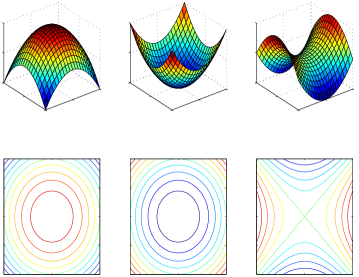
Figure A.1: Morse’s Lemma states that in a neighborhood of a critical point of a Morse function, the level sets are topologically equivalent to one of the three forms (left to right: maximum, minimum, and saddle critical point neighborhoods).

Remark 16

Morse originally used the previous theorem as the definition of Morse functions. This way, a Morse function does not need to be differentiable.

A.2.2 Examples of Morse/non-Morse Functions

Examples of Morse/Non-Morse functions are the following:

• Obviously, $f(x_{1},x_{2})=x_{1}^{2}+x_{2}^{2}$ and $f(x_{1},x_{2})=x_{1}^{2}-x_{2}^{2}$ are Morse Functions.

• The height function $f:S\to\mathbb{R}^{2}$ of the embedding of a compact surface $S\subset\mathbb{R}^{3}$ without boundary is a Morse function. For example, the height function of the torus:

• $f(x_{1},x_{2})=x_{1}^{4}+x_{2}^{4}$ is not a Morse function (degenerate critical point).

• A monkey saddle, i.e., $f(x_{1},x_{2})=x_{1}^{3}-3x_{1}x_{2}^{2}$:

  is not a Morse function (degenerate; level sets of saddle must cross at an ‘X’).

• All non-smooth functions are not Morse functions, e.g. images that have edges!

• Functions that have co-dimension one critical sets (e.g. ridges and valleys) are not Morse functions. Such critical sets are commonplace in images!

A.2.3 Morse Functions are (Almost) all Functions

Morse functions seems to be a very restricted class of functions from the previous examples, however, a basic result from Morse Theory says otherwise.

Definition 15 (Dense Subset of a Normed Space)

Let $\|\cdot\|$ denote a norm on a topological space $X$. A set $S\subset X$ is dense if $\mbox{closure}(S)=X$, i.e., for every $x\in X$ and $\delta>0$, there exists $s\in S$ such that $\|s-x\|<\delta$.

Theorem 11 (Morse Functions are Dense)

Let $\|\cdot\|$ denote the $C^{2}$ norm on the space of $C^{2}$ functions, i.e.,

$$\|f\|=\sup_{x\in\mathbb{R}^{2}}|f(x)|+|\nabla f(x)|+|\nabla^{2}f(x)|.$$

Then Morse functions form an open, dense subset of $C^{2}$ functions.

Remark 17

By the previous theorem, any smooth ($C^{2}$) function can be well approximated by a Morse function up to arbitrary precision (defined by $\|\cdot\|$). For example, ridges and valleys can be approximated with a Morse function, e.g. consider the following circular ridge that can be made Morse by a slight tilt. Let $f(x_{1},x_{2})=\exp{(-(\sqrt{x_{1}^{2}+x_{2}^{2}}-1)^{2})}$ which is a ridge and non-Morse:

Now consider the function $g(x_{1},x_{2})=f(x_{1},x_{2})+\varepsilon x_{1}$, which is arbitrarily close to $f$ (in $C^{2}$ norm) and is a Morse function:

It is a basic fact that $C^{2}$ functions under the norm above are dense in all square integrable functions ($L^{2}$) functions. Therefore, even non-smooth functions can be approximated to arbitrary precision by Morse functions.

A.2.4 Reeb Graph

Definition 16 (Equivalence Relation)

Let $X$ be a set. An equivalence relation on $X$ denoted $\sim$ is a binary relation with the following properties: for all $x,y,z\in X$:

• (reflexivity) $x\sim x$

• (symmetry) if $x\sim y$ then $y\sim x$

• (transitivity) if $x\sim y$ and $y\sim z$, then $x\sim z$

We denote by $[x]$ all elements of $X$ related to $x$, e.g. $[x]=\{y\in X:\,x\sim y\}$.

Definition 17 (Topological Space)

A topology denoted $\mathcal{T}$ on a set $X$ is a collection of subsets of $X$ (called open sets) such that the following properties hold:

• $\emptyset,X\in\mathcal{T}$

• for $U_{\alpha}\in\mathcal{T}$ where $\alpha\in\mathcal{J}$ is an index set (perhaps uncountable), we have $\bigcup_{\alpha\in\mathcal{J}}U_{\alpha}\in\mathcal{T}$.

• for $U_{i}\in\mathcal{T}$ where $i\in\mathcal{I}$ is a finite index set, we have $\bigcap_{i\in\mathcal{I}}U_{i}\in\mathcal{T}$.

Definition 18 (Quotient Space)

Let $X$ be a topological space. Let $\sim$ denote an equivalence relation on $X$. The quotient space of $X$ under the equivalence relation $\sim$, denoted $X/\sim$ is the topological space whose elements are

$$X/\sim\,\doteq\{[x]:\,x\in X\},$$

and whose topology is induced from $X$. The quotient map is the (continuous) function $\pi:X\to X/\sim$ defined by $\pi(x)=[x]$.

Definition 19 (Reeb Graph)

Let $f:\mathbb{R}^{2}\to\mathbb{R}$ be a function. Define a equivalence relation $\sim$ on the space $\mbox{Graph}(f)\doteq\{(x,f(x)):\,x\in\mathbb{R}^{2}\}$ by

$$(x,f(x))\sim(y,f(y))\,\mbox{iff}\,f(x)=f(y)\,\mbox{and there is a continuous path from $x$ to $y$ in $f^{-1}(f(x))$}.$$

The Reeb graph of the function $f$, denoted $Reeb(f)$, is the topological space $\mbox{Graph}(f)/\sim$.

Remark 18

The Reeb graph of a function $f$ is the set of connected components of level sets of $f$ (with the additional information of the function value of each level set).

A.2.5 Examples

We will depict the Reeb graph in the following way: an element $[(x,f(x))]\in\mbox{Reeb}(f)$ will be represented by a point $p_{[(x,f(x))]}$ in the $x-y$ plane, and if $f(z_{1})>f(z_{2})$ then the $y$-coordinate of $p_{[(z_{1},f(z_{1}))]}$ will be larger than $p_{[(z_{2},f(z_{2}))]}$.

• $f(x_{1},x_{2})=x_{1}^{2}+x_{2}^{2}$

• $f(x_{1},x_{2})=\exp{[-(x_{1}^{2}+x_{2}^{2})]}+\exp{[-((x_{1}-1)^{2}+x_{2}^{2})]}$

• $f(x_{1},x_{2})=\exp{[-(x_{1}^{2}+x_{2}^{2})]}-0.1\exp{[-10((x_{1}-0.2)^{2}+x_{2}^{2})]}$

• $f(x,y)=\exp{\left[-(x_{1}^{2}+x_{2}^{2})\right]}+\exp{\left[-((x_{1}-3)^{2}+x_{2}^{2})\right]}+\exp{\left[-((x_{1}+3)^{2}+x_{2}^{2})\right]}$

A.2.6 Properties of Reeb Graphs

Lemma 1 (Reeb graph is connected)

If $f:\mathbb{R}^{2}\to\mathbb{R}$ is a function, then $Reeb(f)$ is connected.

Lemma 2 (Reeb Tree)

If $f:\mathbb{R}^{2}\to\mathbb{R}$ is a function, then $Reeb(f)$ does not contain cycles.

Remark 19

Both of these results follow from basic results in topology, namely, that connectedness and contractibility of loops are preserved under quotienting. That is, since $\mbox{Graph}(f)$ is connected and loops in $\mbox{Graph}(f)$ are contractible (so long as $f$ is continuous), we have that $\mbox{Reeb}(f)=\mbox{Graph}(f)/\sim$ must also have these properties.

Assume now that $f:\mathbb{R}^{2}\to\mathbb{R}$ is a Morse function whose critical points have distinct values, then we may associate an attributed graph to $\mbox{Reeb}(f)$.

Definition 20 (Attributed Graph)

Let $G=(V,E)$ be a graph ($V$ is the vertex set and $E$ is the edge set), and $L$ be a set (called the label set). Let $a:V\to L$ be a function (called the attribute function). We define the attributed graph as $AG=(V,E,L,a)$.

Definition 21 (Attributed Reeb Tree of a Function)

Let $V$ be the set of critical points of $f$. Define $E$ to be

$$E=\{(v_{i},v_{j}):i\neq j,\,\exists\mbox{ a continuous map }\gamma:[0,1]\to Reeb(f)\mbox{ such that }\\ \gamma(0)=[(v_{i},f(v_{i}))],\,\gamma(1)=[(v_{j},f(v_{j}))]\mbox{ and }\gamma(t)\neq[(v,f(v))]\mbox{ for all }v\in V\mbox{ and all }t\in(0,1)\}.$$ (A.1)

Let $L=\mathbb{R}^{+}$, and

$$a(v)=f(v).$$

Definition 22 (Degree of a Vertex)

Let $G=(V,E)$ be a graph, and $v\in V$, then the degree of a vertex, $deg(v)$, is the number of edges that contain $v$.

Theorem 12

Let $f:\mathbb{R}^{2}\to\mathbb{R}^{+}$ be a Morse function with distinct critical values. Let $(V,E,\mathbb{R},f)$ be its Attributed Reeb Tree. Then

1. $(V,E)$ is a connected tree

2. $n_{0}-n_{1}+n_{2}=2$ where $n_{0}$ is the number of maxima, $n_{1}$ the number of saddles and $n_{2}$ the number of minima

3. If $v\in V$ and $v$ is a local minimum/maximum, then $deg(v)=1$

4. If $v\in V$ and $v$ is a saddle, then $deg(v)=3$

Remark 20

Property 2 above is a remarkable fact from Morse Theory, which is more general than it is shown above. Indeed, given a compact surface $S\subset\mathbb{R}^{3}$, the number $n_{0}-n_{1}+n_{2}$ is the same for any Morse function $f:S\to\mathbb{R}^{+}$, i.e., $n_{0}-n_{1}+n_{2}$ (although seemingly a property of the function) is an invariant of the surface $S$.

Remark 21

Using the fact that for any tree $(V,E)$, we have that $|V|-|E|=1$ and Property 2, we can conclude by simple algebraic manipulation that $deg(v)=3$ for a saddle.

Theorem 13 (Stability of Attributed Reeb Tree Under Noise)

Let $f:\mathbb{R}^{2}\to\mathbb{R}$ be a Morse function and set $g_{\varepsilon}=f+\varepsilon h$ where $h:\mathbb{R}^{2}\to\mathbb{R}$ is $C^{2}$. Then for all $\varepsilon$ sufficiently small, $g_{\epsilon}$ is Morse and $ART(f)=ART(g_{\epsilon})$.

A.2.7 Diffeomorphisms and the Attributed Reeb Tree

Definition 23 (Diffeomorphism of the Plane)

A function $\psi:\mathbb{R}^{2}\to\mathbb{R}^{2}$ is a diffeomorphism provided that $\nabla\psi(x)$ and $\nabla\psi^{-1}(x)$ exists for all $x\in\mathbb{R}^{2}$.

Theorem 14 (Invariance of ART Under Diffeomorphisms)

Let $f:\mathbb{R}^{2}\to\mathbb{R}$ be a Morse function and $\psi:\mathbb{R}^{2}\to\mathbb{R}^{2}$ be a diffeomorphism. Then $ART(f)=ART(f\circ\psi)$.

Remark 22

Note that if $p$ is a critical point of $f$, then $\psi^{-1}(p)$ is a critical point of $f\circ\psi$:

$$\nabla(f\circ\psi)(\psi^{-1}(p))=\nabla\psi(\psi^{-1}(p))\circ\nabla f(\psi(\psi^{-1}(p)))=\nabla\psi(p)\circ\nabla f(p)=0\mbox{ if }\nabla f(p)=0.$$

Therefore the vertex set in the ART of both $f$ and $f\circ\psi$ are equivalent. Moreover, if $\gamma$ is a continuous path in $f^{-1}(f(x))$ then $\psi\circ\gamma$ is a continuous path in $(f\circ\psi)^{-1}(f\circ\psi(x))$, as diffeomorphisms do not break continuous paths. Therefore, the edge sets in the ART of $f$ and $f\circ\psi$ are equivalent.

Theorem 15

If $f,g:\mathbb{R}^{2}\to\mathbb{R}$ are Morse functions with distinct critical values and if $ART(f)=ART(g)$, then there exists a monotone function $h:\mathbb{R}\to\mathbb{R}$ and a diffeomorphism $\psi:\mathbb{R}^{2}\to\mathbb{R}^{2}$ such that $f=h\circ g\circ\psi$.

Remark 23

By Morse Lemma, we can construct diffeomorphisms $\psi_{i}$ around critical points, the idea is then to “stitch” these diffeomorphisms up with “patches” to form the diffeomorphism $\psi$ of interest.

Theorem 16 (Reconstruction of Function from ART)

If $(V,E)$ is a tree such that each vertex $v\in V$ is of degree 1 or 3, then there exists a Morse function $f:\mathbb{R}^{2}\to\mathbb{R}$ such that $ART(f)=(V,E)$.

Definition 24 (Orbit Space)

Let $X$ be a set, and $G$ be a group.

• $G$ acts on $X$ if each $g\in G$ is also $g:X\to X$ such that

  1. For each $g,h\in G$ and $x\in X$, $(gh)x=g(hx)$.

  2. For the identity element $e\in G$, we have $ex=x$ for all $x\in X$.

• If $G$ acts on $X$, then the orbit of a point $x\in X$ is $Gx=\{gx:g\in G\}$.

• Define an equivalence relation in $X$ by $x\sim y$ if there exists $g\in G$ such that $gx=y$. The orbit space (or the quotient of the action $G$) is the set $X/G=\{[x]:\,x\in X\}$.

Theorem 17

Let $\mathcal{F}$ be the set of Morse functions with distinct critical values, $\mathcal{H}$ denote the set of monotone functions $h:\mathbb{R}\to\mathbb{R}$, and $\mathcal{W}$ denote the set of diffeomorphisms of the plane. Then

• $\mathcal{H}\times\mathcal{W}$ acts on $\mathcal{F}$ through the action : $(h,w)f\doteq h\circ f\circ w$ for $h\in\mathcal{H}$, $w\in\mathcal{W}$, and $f\in\mathcal{F}$.

• The orbit space $\mathcal{F}/(\mathcal{H}\times\mathcal{W})=\mathscr{T}$ where $\mathscr{T}$ is the set of trees whose vertices have degree 1 or 3.

Remark 24

The second result above is simply a restatement of the Theorems above. Indeed, we can define the mapping $ART:\mathcal{F}/(\mathcal{H}\times W)\to\mathscr{T}$ by

$$ART([f])\doteq ART(f),\mbox{ where }[f]=\{(h,w)f\in\mathcal{F}:\,(h,w)\in\mathcal{H}\times\mathcal{W}\}$$

The function above is well-defined since by Theorem 14, any representative $g\in[f]$ will have the same Attributed Reeb Tree. Note

• Theorem 15 states that $ART:\mathcal{F}/(\mathcal{H}\times W)\to\mathscr{T}$ is injective.

• Theorem 16 states that $ART:\mathcal{F}/(\mathcal{H}\times W)\to\mathscr{T}$ is surjective.

• Therefore, $ART:\mathcal{F}/(\mathcal{H}\times W)\to\mathscr{T}$ is a bijection and therefore, $\mathcal{F}/(\mathcal{H}\times W)=\mathscr{T}$.

A.3 Radiometry primer (by Paolo Favaro)

We describe the light source using its radiance, ${R_{L}}(q,{l})$, which indicates the power density per unit area and unit solid angle emitted at a point $q\in L$ in a given direction ${l}\in{\mathbb{H}}^{2}$, and is measured in [W/sterad/$m^{2}$]. This is a property of the light source. When we consider the particular direction ${l}$ from a point $q\in L$ on the light source towards a point $p\in S$ on the scene, this is given by ${g_{q}}_{*}(p-q)=g_{q}p-0=g_{q}p$. Therefore, given a solid angle $d\Omega_{L}$ and an area element $dL$ on the light source, the power per solid angle and unit foreshortened area radiated from a point $q$ towards $p$ is given by

$${R_{L}}(q,g_{q}p)d\Omega_{L}\langle\nu_{q},g_{q}p\rangle dL$$ (A.2)

where $g_{q}p\in{\mathbb{H}}^{2}$ is intended as a unit vector. Now, how big a patch $dL$ of the light we see standing at a point $p$ on the scene depends on the solid angle $d\Omega_{S}$ we are looking through. Following Figure A.2 we have that

$$dL=d\Omega_{S}\|p-q\|^{2}/\langle\nu_{q},l_{qp}\rangle$$ (A.3)

where we have defined $l_{qp}\doteq q-p/\|q-p\|$ and the inner product at the denominator is called foreshortening. Similarly, the solid angle $d\Omega_{L}$ shines a patch of the surface $dS$. The two are related by

$$d\Omega_{L}=\frac{dS}{\|p-q\|^{2}}\langle\nu_{q},l_{pq}\rangle$$ (A.4)

where $l_{pq}=-l_{qp}=p-q/\|p-q\|$. Substituting the expressions of $d\Omega_{L}$ and $dL$ in the previous two equations into (A.2), one obtains the infinitesimal power received at the point $p$.

Figure A.2: Energy balance: a light source patch $dL$ radiates energy towards a surface patch $dS$. Therefore, the power injected in the solid angle $d\Omega_{L}$ by $dL$ equals the power received by $dS$ in the solid angle $d\Omega_{S}$. Equation (A.4) expresses this balance in symbols.

Now, we want to write the portion of power exiting the surface at $p$ in the direction of a pixel ${x}$ through an area element $dS$. First, we need to write the direction of ${x}$ in the local reference frame at $p$. We assume that ${x}$ is a unit vector, obtained for instance via central perspective projection

$$\pi:\mathbb{R}^{3}\longrightarrow{\mathbb{S}}^{2};\ p\mapsto\pi(p)\doteq{x}.$$ (A.5)

However, the point $p$ is written in the inertial frame, while ${x}$ is written in the frame of the camera at time $t$. We need to first transform ${x}$ to the inertial frame, via $g_{*}(t)^{-1}{x}$, and then express this in the local frame at $p$, which yields ${g_{p}}^{-1}_{*}g_{*}(t)^{-1}{x}$. We call the normalized version of this vector $l_{p{x}}(t)$. Then, we need to integrate the infinitesimal power radiated from all points on the light source through their solid angle $d\Omega_{L}$ against the BRDF, which specifies what portion of the incoming power is reflected towards ${x}$. This yields the infinitesimal energy that $p$ radiates in the direction of ${x}$ through an area element $dS$:

$${R_{S}}(p,{x})dS(p)=\int_{L}\beta(l_{p{x}}(t),g_{p}q){R_{L}}(q,g_{q}p)d\Omega_{L}(q)\langle\nu_{q},g_{q}p\rangle dL(q)$$ (A.6)

where the arguments in the infinitesimal forms $dS,dL,d\Omega_{L}$ indicate their dependency. Now, we can substitute the expression of $d\Omega_{L}$ from (A.4) and simplify the area element $dS$, to obtain the radiance of the surface at $p$

$${R_{S}}(p,{x})=\int_{L}\beta(l_{p{x}}(t),g_{p}q){R_{L}}(q,g_{q}p)\frac{\langle\nu_{q},g_{q}p\rangle}{\|p-q\|^{2}}\big{\langle}N_{p},l_{pq}\big{\rangle}dL(q)$$ (A.7)

Since the norm $\|p-q\|$ is invariant to Euclidean transformations, we can write it as $\|g_{q}p\|$. Now, if the size of the scene is small compared to its distance to the light, this term is almost constant, and therefore the measure

$$dE(q,g_{q}p)\doteq{R_{L}}(q,g_{q}p)\frac{\langle\nu_{q},g_{q}p\rangle}{\|g_{q}p\|^{2}}dL(q)$$ (A.8)

can be thought of as a property of the light source. Since we cannot untangle the contribution of ${R_{L}}$ from that of $dL$, we just choose $dE$ to describe the power distribution radiated by the light source. Therefore, we have

$${R_{S}}(p,{x})=\int_{L}\beta(l_{p{x}}(t),g_{p}q)\big{\langle}N_{p},l_{pq}\big{\rangle}dE(q,g_{q}p).$$ (A.9)

This is the portion of power per unit area and unit solid angle radiated from a point $p$ on a reflective surface towards a point ${x}$ on the image at time $t$. The next step consists of quantifying what portion of this energy gets absorbed by the pixel at location ${x}$. This follows a similar calculation, which we do not report here, and instead refer the reader to [78] (page 208). There, it is argued that the irradiance at the pixel ${x}$ is equal to the radiance at the corresponding point $p$ on the scene, up to an approximately constant factor, which we lump into ${R_{S}}$. The point $p$ and its projection ${x}$ onto the image plane at time $t$ are related by the equations

$${x}=\pi(g(t)p)\quad p=g(t)^{-1}\pi_{S}^{-1}({x})$$ (A.10)

where $\pi_{S}^{-1}:{\mathbb{S}}^{2}\rightarrow\mathbb{R}^{3}$ denotes the inverse projection, which consists in scaling ${x}$ by its depth $Z({x})$ in the current reference frame, which naturally depends on $S$. Therefore, the equation below, known as the irradiance equation, takes the form

$$I({x},t)={R_{S}}(p,\pi(g(t)p))={R_{S}}(g(t)^{-1}\pi_{S}^{-1}({x}),{x}).$$ (A.11)

After we substitute the expression of the radiance (A.9), we have the imaging equation, which we describe in Section B.1, Equation (B.7).

Appendix B

B.1 Basic image formation

This section spells out the conditions under which the Ambient-Lambert-Static model is a reasonable approximation of the image formation process.

B.1.1 What is the “image” …

An “image” is just an array of positive numbers that measure the intensity (irradiance) of light (electromagnetic radiation) incident a number of small regions (“pixels”) located on a surface. We will deal with gray-scale images on flat, regular arrays, but one can easily extend the reasoning to color or multi-spectral images on curved surface, for instance omni-directional mirrors. In formulas, a digital image is a function $I:[0,N_{x}-1]\times[0,N_{y}-1]\rightarrow[0,N_{g}-1];\ (x,y)\mapsto I(x,y)$ for some number of horizontal and vertical pixels $N_{x},N_{y}$ and grey levels $N_{g}$. For simplicity, we neglect quantization in both pixels and gray levels, and assume that the image is given on a continuum $D\subset\mathbb{R}^{2}$, with values in the positive reals:

$$I:D\subset\mathbb{R}^{2}\rightarrow\mathbb{R}_{+};\ {x}\mapsto I({x})$$ (B.1)

where ${x}\doteq[x,\ y]^{T}\in\mathbb{R}^{2}$. When we consider more than one image, we index them with $t$, which may indicate time, or generically an index when images are not captured at adjacent time instants: $I({x},t)$. We often use time as a subscript, for convenience of notation: $I_{t}({x})$. This abstraction in representing images is all we need for the purpose of this manuscript.

B.1.2 What is the “scene”…

A simple description of the “scene”, or the “object”, is less straightforward. This is a modeling task, for which there is no right or wrong choice, and finding a suitable model is as much an art as it is a science; one has to exercise discretion to strike a compromise between simplicity and realism. We consider the scene as a collection of “objects” that are volumes bounded by closed, piecewise smooth surfaces embedded in $\mathbb{R}^{3}$. We call the generic surface $S$, which may for convenience be separated into a number $i=1,\dots,N_{o}$ of simply connected components, or “objects” $S=\cup_{i=1}^{N_{o}}S_{i}$. The surface is described relative to a (Euclidean) reference frame, which we call $g\in SE(3)$. The two entities

$$S\subset\mathbb{R}^{3};\ g\in SE(3)$$ (B.2)

describe the geometry of the scene, and in particular we call $g$ the pose relative to a fixed (or “inertial”) reference frame and $S$ the shape of objects, although a more proper definition of shape would be the quotient $S/g$ [96]. This is, however, inconsequential as far as our discussion is concerned.

Objects interact with light in ways that depend upon their material properties. Describing the interaction of light with matter can be rather complicate if one seeks physical realism: one would have to start from Maxwell’s equations and describe the scattering properties of the volume contained in each object. That is well beyond our scope. Besides, we do not seek physical realism, but only to capture the phenomenology of the material to the extent in which it can be used for detection, recognition or other visual decision tasks. We will therefore start from a much simpler model, one that is popular in computer graphics, because it can describe with sufficient accuracy a sufficient number of real-world objects: each point $p$ on an object $S$ has associated with it a function $\beta:{\mathbb{H}}^{2}\times{\mathbb{H}}^{2}\rightarrow\mathbb{R}_{+};(v,{l})\mapsto\beta(v,{l})$ that determines the portion of energy coming from a direction ${l}$ that is reflected in the direction $v$, each represented as a point on the half-sphere ${\mathbb{H}}^{2}$ centered at the point $p$. This is called the bi-directional reflectance distribution function (BRDF) and is measured in [1/sterad]. This model neglects diffraction, absorption, subsurface scattering; it only describes the reflective properties of materials (reflectance).

To make the notation more precise, we define a local (Euclidean) reference frame, centered at the point $p$ with the third axis along the normal to the surface, $e_{3}=N_{p}\perp T_{p}S$ and first two axes parallel to the tangent plane.

Figure B.1: Local reference frame at the point $p$.

We call such a local reference frame $g_{p}$, which is described in homogeneous coordinates by

$$g_{p}=\left[\begin{array}[]{cc}\left[\begin{array}[]{ccc}u_{p}&v_{p}&N_{p}\end{array}\right]&p\\ 0&1\end{array}\right]$$ (B.3)

where $u_{p}$, $v_{p}$ and $N_{p}$ are unit vectors. Therefore, a point $q$ in the inertial reference frame will transform to $g_{p}q$ in the local frame at $p$. Similarly, a vector $v$ in the inertial frame will transform to ${g_{p}}_{*}v$ in the local frame where

$${g_{p}}_{*}=\left[\begin{array}[]{cc}\left[\begin{array}[]{ccc}u_{p}&v_{p}&N_{p}\end{array}\right]&0\\ 0&0\end{array}\right].$$ (B.4)

The total energy radiated by the point $p$ in a direction $v$ is obtained by integrating, of all the energy coming from the light source, the portion that is reflected towards $v$, according to the BRDF. The light source is the collection of objects that can radiate energy. In principle, every object in the scene can radiate energy (either by reflection or by direct radiation), so the light source is just the scene itself, $L=S$, and the energy distribution can be described by a distribution of directional measures on $L$, which we call $dE\in{L}_{\rm loc}(L\times\mathbb{H}^{2})$, the set of locally integrable distributions on $L$ and the set of directions. These include ordinary functions as well as ideal delta measures. The distribution $dE$ depends on the properties of the light source, which is described by a function ${R_{L}}:L\times\mathbb{H}^{2}\rightarrow\mathbb{R}$ of the point $q$ on the light source and a direction (see Appendix A.3 for the relationship between $dE$ and ${R_{L}}$). The collection

$$\beta(\cdot,\cdot):{\mathbb{H}}^{2}\times{\mathbb{H}}^{2}\rightarrow\mathbb{R}_{+};\ L\ {\rm and}\ dE:L\times\mathbb{H}^{2}\rightarrow\mathbb{R}_{+}$$ (B.5)

describes the photometry of the scene (reflectance and illumination). Note that $\beta$ depends on the point $p$ on the surface, and we are imposing no restrictions on such a dependency. For instance, we do not assume that $\beta$ is constant with respect to $p$ (homogeneous material). When emphasizing such a dependency we write $\beta(v,{l};p)$.

In addition, reflectance (BRDF) and geometry (shape and pose) are properties of each object that can change over time. So, in principle, we would want to allow $\beta,\ S,\ g$ to be functions of time. In practice, we assume that the material of each object does not change, but only its shape, pose and of course illumination. Therefore, we will use

$$S=S(t);\ g=g(t),\ \ t\in[0,T]$$ (B.6)

to describe the dynamics of the scene. The index $t$ can be thought of as time, in case a sequence of measurements is taken at adjacent instants or continuously in time, or it can be thought of as an index if disparate measurements are taken under varying conditions (shape and pose). We often indicate the index $t$ as a subscript, for convenience: $S_{t}\doteq S(t);\ g_{t}\doteq g(t)$. Note that, as we mentioned, the light source $(L,dE)$ can also change over time. When emphasizing such a dependency we write $L(t)$ and $dE(q,{l};t)$, or $L_{t},dE_{t}({l})$.

Example 8

The simplest surface $S$ one can conceive of is a plane: $S=\{p\in\mathbb{R}^{3}\ |\ \langle N,p\rangle=d\}$ where $N$ is the unit normal to the plane, and $d$ is its distance to the origin. For a plane not intersecting the origin, $1/d$ can be lumped into $N$, and therefore three numbers are sufficient to completely describe the surface in the inertial reference frame. In that case we simply have $S$ a constant, and $g=e$, the identity. A simple light source is an ideal point source, which can be modeled as $L\in\mathbb{R}^{3}$ with infinite power density $dE=E_{l}\delta(q-L)dL(q)$. Another common model is a constant ambient illumination, which can be modeled as a sphere $L={\mathbb{S}}^{2}$ with $dE=E_{0}dL$. We will discuss examples of various models for the BRDF shortly.

Remark 25 (Choosing a level of granularity in the representation)

Note that by assuming that the world is made of surfaces we are already imposing significant restrictions, and we are implicitly choosing a level of granularity for our representation. Consider for instance the fabric shown in Figure B.2. There is no surface there. The fabric is made of thin one-dimensional threads, just woven tightly enough to give the impression of spatial continuity. Therefore, we choose to represent them as a smooth surface. Of course, the variation in the appearance due to the fine-scale structure of the threads has to be captured somehow, and we delegate this task to the reflectance model. Naturally, one could even describe each individual thread as a cylindrical surface modeled as an object $S$, but this is well beyond the level of detail that we want to capture. This example illustrates the fact that describing objects entails a notion of scale. Something (e.g. a thread) is an object at one scale, but is merely part of a texture at a coarser scale. Figure B.2 highlights the modeling tradeoff between shape and reflectance: one could model the fabric as a very complex object (woven thread) made of homogeneous material (wool), or as a relatively simple object (a smooth surface) made of textured material. Although physically different, these two scenarios are phenomenologically indistinguishable, which relates to the discussion earlier in the manuscript of the role between the light field and the complete representation.

Figure B.2: A complex shape (woven thread) with simple reflectance (homogeneous material), or a simple shape (a smooth surface) with complex reflectance (texture)?

Remark 26 (Tradeoff between shape and motion)

As we have already noted, instead of allowing the surface $S$ to deform arbitrarily in time via $S(t)$, and moving rigidly in space via $g(t)\in SE(3)$, we can lump the motion and deformation into $g(t)$ by allowing it to belong to a more general class of deformations $G$, for instance diffeomorphisms, and let $S$ be constant. Alternatively, we can lump the deformation $g(t)$ into $S$ and just describe the surface in the inertial reference frame via $S(t)$. This can be done with no loss of generality, and it reflects a fundamental tradeoff in modeling the interplay between shape and motion [163].

Now, if we agree that a scene can be described by its geometry, photometry and dynamics, we must decide how these relate to the measured images.

B.1.3 And how are the two related?

Given a description of the geometry, photometry and dynamics of a scene, a model of the image is obtained through a description of the imaging device. An imaging device is a series of elements designed to control light propagation. This is typically modeled through diffraction, reflection, and refraction. We ignore the first two, and only consider the effects of refraction. For simplicity, we can also assume that the set of objects that act as light sources and those that act as light sinks are disjoint, so that $S\cap L=\emptyset$, i.e. we ignore inter-reflections. Note that $S$ needs not be simply connected, so we can divide simply connected regions of the scene into “light” $L$ and “objects” $S_{i},\ i=1,\dots,N_{o}$.

Now, using the notation introduced in the previous section, we want to determine the energy that impinges on a given pixel as a function of the shape of the scene $S$, its BRDF $\beta$, the light source $L$ and its energy distribution $dE$, and the position and orientation of the camera. For simplicity, given the tradeoff between shape and motion discussed in Remark 26, we describe the (possibly time-varying) shape of the scene in the inertial frame and drop the explicit description of its pose. In fact, to further simplify the notation, we can choose the inertial frame to coincide with the position and orientation of the viewer at time $t=0$, so that if $I_{0}({x}_{0})$ is the first image, then the scene can be described as a surface parameterized by ${x}_{0}$: $S_{t}({x}_{0})$. We then describe the position and orientation of the camera at time $t$ relative to the camera at time $0$ using a moving Euclidean reference frame $g_{t}\in SE(3)$. Following the derivation in Appendix A.3, the intensity (irradiance) measured at a pixel ${x}$ on the image indexed by $t$ is given by

$$\boxed{\begin{cases}I_{t}({x})=\int_{L}\beta(l_{p{x}}(t),g_{p}q)\big{\langle}N_{p},l_{pq}\big{\rangle}dE(q,g_{q}p);\\ {x}=\pi(g_{t}p);\ p\in S\end{cases}}~{}~{}~{}~{}~{}{\rm The\ Imaging\ Equation}$$ (B.7)

where the symbols above are defined as follows:

Directions:

In the equation above, we have defined $l_{p{x}}\doteq{g_{p}}^{-1}_{*}g_{*}(t)^{-1}{x}$, $g_{p}$ and ${g_{p}}_{*}$ are defined by Equation (B.3) and (B.4) respectively, $l_{pq}\doteq p-q/\|p-q\|$ and $g_{p}q$ indicates the (normalized) direction from $p$ to $q$, and similarly for $g_{q}p$;

Light source:

$L\subset\mathbb{R}^{3}$ is the (possibly time-varying) collection of light sources emitting energy with a distribution $dE:L\times{\mathbb{H}}^{2}\rightarrow\mathbb{R}_{+}$ at every point $q\in L$ towards the direction of a point $p$ on the

Scene:

a collection of (possibly time-varying) piecewise smooth surfaces $S\subset\mathbb{R}^{3}$; $\beta:{\mathbb{H}}^{2}\times{\mathbb{H}}^{2}\times S\rightarrow\mathbb{R}$ is the bi-directional reflectance distribution function (BRDF) that depends on the incident direction, the reflected direction and the point $p\in S$ on the scene $S$ and is a property of its material.

Motion:

relative motion between the scene and the camera is described by the motion of the camera $g_{t}\in SE(3)$ and possibly the action of a more complex group $G$, or simply by allowing the surface $S_{t}$ to change over time.

Projection:

$\pi:\mathbb{R}^{3}\mapsto{\mathbb{S}}^{2}$ denotes ideal (pinhole) perspective projection, modeled here as projection onto the unit sphere, although the same model applies if $\pi:\mathbb{R}^{3}\rightarrow{\mathbb{P}}^{2}$, in which case $l_{p{x}}$ has to be normalized accordingly.

Visibility and cast shadows:

One should also add to the equation two characteristic function terms: $\chi_{v}({x},t)$ outside the integral, which models the visibility of the scene from the pixel ${x}$, and $\chi_{s}(p,q)$ inside the integral to model the visibility of the light source from a scene point (cast shadows). We are omitting these terms here for simplicity. However, in some cases that we discuss in the next section, discontinuities due to visibility or cast shadows can be the only source of visual information.

Remark 27 (A philosophical aside on scene modeling)

One could argue that the real world cannot be captured by simple mathematical models of the type just described, and even classical physics is largely inadequate for the task. However, we are not looking for an absolute model. Instead, we are looking to describe the scene at the level of granularity that is suitable for us to be able to perform inference and accomplish certain tasks. So, what is the “right” granularity? For us a suitable model of the scene is one that can be validated with other existing sensing modalities, for instance touch. This is well illustrated by the fabric of Figure B.2, where at the level of granularity required the scene can be safely described as a smooth surface. Notice that this is similar to what other researchers have suggested by describing the scene as a functional that cannot be directly measured. However, such a functional can be evaluated with various test-functions. Physical instruments provide a set of test functions, and imaging device provide yet another set of test functions. The goal of the imaging model, therefore, can be thought of as relating the value of the scene functional obtained by probing with physical instruments to the value obtained by probing with images.

The imaging equation is relevant because most of computer vision is about inverting it; that is, inferring properties of the scene (shape, material, motion) regardless of pose, illumination and other nuisances (the visual reconstruction problem). However, in the general formulation above, one cannot infer photometry, geometry and dynamics from images alone. Therefore, we are interested in deriving a model that strikes a balance between tractability (i.e. it should contain only parameters that can be identified) and realism (i.e. it should capture the phenomenology of image formation). We will use simple models that are widely used in computer graphics to generate realistic, albeit non-perfect, images: Phong (corrected) [141], Ward [190] and Torrance-Sparrow (simplified) [177]. All these models include a function $\rho_{d}(p)$ called (diffuse) albedo, and a function $\rho_{s}(p)$ called specular albedo. Diffuse albedo is often called just albedo, or, improperly, texture. In the next section we discuss various special cases of the imaging equation and the role they play in visual reconstruction. Here we limit ourselves to deriving the model under a generic illumination consisting of an ambient term and a number of concentrated point light sources at infinity: $L={\mathbb{S}}^{2}\cup\{L_{1},L_{2},\dots,L_{k}\},\ L_{i}\in{\mathbb{R}}^{3}$, $dE(q)=E_{0}dL(q)+\sum_{i=1}^{k}E_{i}\delta(q-L_{i})$. In this case the imaging equation reduces to

$$\boxed{\begin{cases}I_{t}({x})=\rho_{d}(p)\left(E_{0}+\sum_{i=1}^{k}E_{i}\langle N_{p},L_{i}\rangle\right)+\rho_{s}(p)\sum_{i}E_{i}\frac{\big{\langle}g_{t}^{-1}{x}+L_{i}/\|L_{i}\|,N_{p}\big{\rangle}^{c}}{\langle g_{t}^{-1}{x},N_{p}\rangle}\\ {x}=\pi(g_{t}p);\quad p=S({x}_{0}).\end{cases}}$$ (B.8)

Remark 28

Note that this model does not explicitly include occlusions and shadows. Also, note that the first (diffuse) term does not depend on the viewpoint $g$, whereas the second term (specular) does. However, note that, depending on the coefficient $c$, the second term is only relevant when ${x}$ is close to the specular direction and, therefore, if one assumes that the light sources are concentrated, the second term is relevant in a small subset of the scene. If we threshold the effects of the second term based on the angle between the viewing and the specular direction, then we can write the above model as

$$I_{t}({x})=\begin{cases}\rho_{d}(p)\left(E_{0}+\sum_{i=1}^{k}E_{i}\langle N_{p},L_{i}\rangle\right)~{}~{}~{}{\rm if}~{}~{}\big{\langle}g_{t}^{-1}{x}+L_{i}/\|L_{i}\|,N_{p}\big{\rangle}<\gamma(c)\ \forall\ i\\ \rho_{s}(p)E_{\hat{i}}~{}~{}~{}{\rm otherwise}\end{cases}$$ (B.9)

where $\hat{i}=\arg\min_{i}\frac{\big{\langle}g_{t}^{-1}{x}+L_{i}/\|L_{i}\|,N_{p}\big{\rangle}^{c}}{\langle g_{t}^{-1}{x},N_{p}\rangle}$ which justifies the rank-based model of [88]. Empirical evaluation of the validity of this model, and the resulting “brightness constancy constraint,” discussed in the next subsection, has not been thoroughly addressed in the literature.

The “identity” of a scene or an object is specified by its shape $S$ and its reflectance properties $\beta$. The illumination $L(t),dE(\cdot,t)$, visibility $\chi({x},t)$ and pose/deformation $g(t)$ are “nuisance factors” that affect the measurements but not the identity of the scene/object. They change with the view, whereas the identity of the object does not. In the imaging equation (B.8) we measure $I_{t}({x})$ for all ${x}\in D$ and $t=t_{1},t_{2},\dots,t_{m}$, and the unknowns are $L(t_{j}),dE(\cdot,t_{j}),g(t_{j})$, which for simplicity we indicate as $L_{j},dE_{j}(\cdot),g_{j}$ respectively, for all $j=1,\dots,m$. For simplicity, we indicate all the unknowns of interest with the symbol $\xi$ (note that some unknowns are infinite-dimensional), and all the nuisance variables with $\nu$. Equation (B.8), once we write the coordinates of the point $p$ relative to the pixel in the moving frame, $p=g(t)^{-1}\pi^{-1}({x},t)$, can then be written as a functional $h$, formally, as follows:

$$\boxed{I=h(\xi,\nu)+n.}~{}~{}~{}{\rm The\ Imaging\ Equation\ Lite}$$ (B.10)

∑ where, to summarize the equivalence of (B.10) with (B.8), we have

$$\begin{cases}I:D\subset\mathbb{R}^{2}\rightarrow\mathbb{R}^{3}\\ \xi\in C(\mathbb{R}^{2}\backslash{\cal D}\rightarrow\mathbb{R}^{3})\times BV({\mathbb{S}}^{2}\times{\mathbb{S}}^{2}\rightarrow\mathbb{R}^{+})\doteq{\cal S}\\ \nu\in SE(3)\times BV(\mathbb{R}^{3}\rightarrow\mathbb{R}^{+})\times{\mathbb{P}}(\mathbb{R}^{3}\rightarrow\mathbb{R}^{2})\doteq{\cal\nu}\\ h:\mathbb{R}^{3}\times BV(\mathbb{R}^{3}\rightarrow\mathbb{R}^{+})\times SE(3)\times\mathbb{R}^{+}\times\mathbb{R}^{3k}\times\mathbb{R}^{k}\rightarrow\mathbb{R}^{+}\\ ~{}~{}~{}~{}~{}~{}~{}(p,\beta,g,E_{0},\{L_{1},\dots,L_{k}\},\{E_{1},\dots,E_{k}\})\mapsto I\\ n\sim{\cal N}(0,Q)\end{cases}$$ (B.11)

where $\cal D$ is a subset of measure zero (the set of discontinuities), $BV$ denotes functions of bounded variation. We will use the symbolic notation of (B.10) and the explicit notation of (B.8) interchangeably, depending on convenience. In some cases we may indicate the arguments of the functions $I,\xi,\nu,n$ explicitly.

Remark 29 (Occlusions and cast shadows)

Occlusions are an accident of image formation that significantly complicates our modeling efforts. In fact, while they are “nuisances” in the sense that they do not depend solely on the scene, the do depend on both the scene and the viewpoint (for occlusions) and illumination (for cast shadows). That is why, despite depending on the nuisance, under suitable conditions they can be exploited to infer the shape of the scene (see [200] for occlusions and [25] for cast shadows). For the case of illumination, as we will show, there is no loss of generality in assuming ambient + point-light illumination, at which point cast shadows are simple to model as a selection process of what sources are visible from each point. Nevertheless, it is a global inference problem that requires a global solution.

B.2 Special cases of the imaging equation and their role in visual reconstruction (taxonomy)

In its general formulation above, the imaging equation cannot be inverted. Therefore, it is common to make assumptions on some of the unknowns in order to recover the others. In this section we aim at enumerating a collection of special cases that compounded characterize most of what can be done in visual inference. We start with models of reflection.

Many common materials can be fruitfully described by a BRDF. Exceptions include translucent materials (e.g. skin), anisotropic material (e.g. brushed aluminum), micro-structured material (e.g. hair) etc. However, since our goal is not realism in a physical simulation, we are content with some common BRDF that are well established in computer graphics: Phong (corrected) [141], Ward [190] and Torrance-Sparrow (simplified) [177].

Phong (corrected)

$\beta(v,{l})=\rho_{d}(p)+\rho_{s}(p)\cos^{c}\delta/\cos\theta_{i}\cos\theta_{o}$.
Here $\cos\delta=\langle g(t)^{-1}{x}+q/\|q\|,N_{p}\rangle$ where each term in the inner product is normalized, and $\theta_{i}\doteq\arccos\langle{l},N_{p}\rangle$, and $\arccos(\theta_{o})\doteq\langle v,N_{p}\rangle$; $c\in\mathbb{R}$ is a coefficient that depends on the material.

Ward

$\beta(v,{l})=\rho_{d}(p)+\rho_{s}(p)\frac{\exp(-\tan^{2}(\delta)/\alpha^{2})}{\sqrt{\cos\theta_{i}\cos\theta_{o}}}$.
Here $\alpha\in\mathbb{R}$ is a coefficient that depends on the material and is determined empirically.

Torrance-Sparrow (simplified)

$\beta(v,{l})=\rho_{d}(p)+\rho_{s}(p)\frac{\exp(-\delta^{2}/\alpha^{2})}{\cos\theta_{i}\cos\theta_{o}}$.

Separable radiance

As Nayar and coworkers point out [134], the radiance for the latter model can be written as the sum of products, where the first factor depends solely on material (diffuse and specular albedo), whereas the second factor compounds shape, pose and illumination.

In all these cases, $\rho_{d}(p)$ is an unknown function called (diffuse) albedo, and $\rho_{s}(p)$ is an unknown function called specular albedo. Diffuse albedo is often called just albedo, or, improperly, texture.

Note that the first term (diffuse reflectance) is the same in all three models. The second term (specular reflectance) is different. Surfaces whose reflectance is captured by the first term are called Lambertian, and are by far the most studied in computer vision.

B.2.1 Lambertian reflection

Lambertian surfaces essentially look the same regardless of the viewpoint: $\beta(v,{l})=\beta(w,{l})\ \forall w\in{\mathbb{H}}^{2}$. This yields major simplifications of the image formation model. Moreover, in the case of constant illumination, it allows relating different views of the same scene to one another directly, bypassing the image formation model. This is known as the local correspondence problem, which relies crucially on the Lambertian assumption and the resulting brightness constancy constraint. We address this case first.

Constant illumination

In this case we have $L(t)=L$ and $dE(q,{l};t)=dE(q,{l})$. We consider two simple light source models first.

Self-luminous

Ambient light is due to inter-reflection between different surfaces in the scene. Since modeling such inter-reflections is quite complicated, we will approximate it by assuming that there is a constant amount of energy that “floods” the ambient space. This can be approximated by a (half) sphere radiating constant energy: $L={\mathbb{S}}^{2}$ and $dE=E_{0}dL$. In this case, the imaging equation reduces to

$$I({x},t)=\rho_{d}(p)E_{0}\int_{{\mathbb{S}}^{2}}\langle N_{p},{l}\rangle d\Omega({l})\doteq E(p).$$ (B.12)

Due to the symmetry of the light source, assuming there are no shadows and having a full sphere, we can always change the global reference frame so that $N_{p}=e_{3}$. However, it is only to first approximation (for convex objects) that the integral does not depend on $p$, i.e. we can neglect vignetting. In this case, $E_{0}$ can be lumped into $\rho_{d}$, yielding the simplest possible model that, when written with respect to a moving camera, gives

$$\boxed{\begin{cases}I({x},t)=\rho(p)\\ {x}=\pi(g(t)p);\quad p=S({x}_{0}).\end{cases}}$$ (B.13)

Note that this model effectively neglects illumination, for one can think of a scene $S$ that is self-luminous, and radiates an equal amount of energy $\rho(p)$ in all directions. Even for such a simple model, however, performing visual inference is non-trivial. It has been done for a number of special cases:

Constant albedo: silhouettes

When $\rho(p)$ is constant, the only information in Equation (B.13) is at the discontinuities between ${x}=\pi(g(t)p),p\in S$ and $p\notin S$, i.e. at the occluding boundaries. Given suitable conditions, that have been first studied by Aström et al. [7], motion $g(t)$ and shape $S$ can be recovered. The reconstruction of shape $S$ and albedo $\rho$ has been addressed in an infinite-dimensional optimization framework by Yezzi and Soatto [198, 201] in their work on stereoscopic segmentation.

Smooth albedo

The stereoscopic segmentation framework has been extended to allow the albedo to be smooth, rather than constant. The algorithm in [89] provides an estimate of the shape of the scene $S$ as well as its albedo $\rho(p)$ given its motion relative to the viewer, $g(t)$.

Piecewise constant/piecewise smooth albedo

The same framework has been recently extended to allow the albedo to be piecewise constant in [86]. This amount to performing region-based segmentation a’ la Mumford-Shah [131] on the scene surface $S$. Although it has not been done yet, the same ideas could be extended to piecewise smooth albedo.

Nowhere constant albedo

When $\nabla\rho(p)\neq 0$ everywhere in $p$, the image formation model can be bypassed altogether, leading to the so-called correspondence problem which we will see shortly. This is at the base of most traditional stereo reconstruction algorithms and structure from motion. Since these techniques apply without regard to the illumination, we will address this after having relaxed our assumptions on illumination.

Point light(s)

A countable number of stationary point light sources can be modeled as $L=\{L_{1},L_{2},\dots,L_{k}\},\ L_{i}\in\mathbb{R}^{3}$, $dE=\sum_{i=1}^{k}E_{i}\delta(q-L_{i})$. In this case the imaging equation reduces to

$$I({x},t)=\sum_{i=1}^{k}E_{i}\rho_{d}(p)\langle N_{p},p-L_{i}/\|p-L_{i}\|\rangle.$$ (B.14)

Note that, if we neglect occlusions and cast shadows, the sum can be taken inside the inner product and therefore there is no loss of generality in assuming that there is only one light source. If the light sources are at infinity, $p$ can be dropped from the inner product; furthermore, the intensity of the source $E$ multiplies the light direction, so the two can be lumped into the vector $L$. We can therefore further simplify the above model to yield, taking into account camera motion,

$$\boxed{\begin{cases}I({x},t)=\rho(p)\langle N_{p},L\rangle\\ {x}=\pi(g(t)p);\quad p=S({x}_{0})\end{cases}}$$ (B.15)

Inference from this model has been addressed for the following cases.

Constant albedo

Yuille et al. [203] have shown that given enough viewpoints and lighting positions one can reconstruct the shape of the scene. Jin et al. [86] have proposed an algorithm for doing so, which estimates shape, albedo and position of the light source in a variational optimization framework. If the position of the light source is known and there is no camera motion, this problem reduces to classical shape from shading [77].

Smooth/piecewise smooth albedo

In this case, one can easily show that albedo and light source cannot be recovered since there are always combinations of the two that generate the same images. However, under suitable conditions shape can still be estimated, as we discuss next.

Nowhere constant radiance

If the combination of albedo and the cosine term (the inner product in (B.15)) result in a radiance function that has non-zero gradient, we can think of the radiance as an albedo under ambient illumination, and therefore this case reduces to multi-view stereo, which we will discuss shortly. Naturally, in this case we cannot disentangle reflectance from illumination, but under suitable conditions we can still reconstruct the shape of the scene, as we discuss shortly in the context of the correspondence problem.

Cast shadows

If the visibility terms are included, under suitable conditions about the shape of the object and the number and nature of light sources, one can reconstruct an approximation of the shape of the scene.

General light distribution: the reflectance/illumination ambiguity

As we have already discussed, in the absence of mutual illumination the light source $L$ and the scene $S$ are disjoint. We make the assumption that the light source is “far,” i.e. the minimum distance between $L$ and $S$ is much smaller than the maximum distance between two points in $S$, $\min_{p\in S,q\in L}d(p,q)>>\max_{p,r\in S}d(p,r)$. Under these assumptions, we can approximate the light source with a half-sphere with infinite radius, $L={\mathbb{H}}^{2}(\infty)$. The radiance of the light source therefore only depends on the position $q\in L$, but not on the direction, since the latter is always normal to $L$; therefore, $dE:L\rightarrow\mathbb{R}_{+};\ q\mapsto dE(q)\geq 0$. An image is obtained by integrating the light source against the BRDF:

$$I(x)=\int_{L}\beta_{p}(x,\lambda)dE(\lambda)=\int_{{\mathbb{H}}^{2}}\beta_{p}(\nu_{px},\lambda)e(\lambda)dS$$ (B.16)

where $dS$ is the area form of the sphere, and we neglect edge effects. For notational simplicity we write $\beta_{p}(x,\lambda)$ as a short-hand for $\beta_{p}(\nu_{px},\nu_{p\lambda})$. Clearly, if we call $\tilde{\beta}_{p}(x,\lambda)\doteq\beta_{p}(x,\lambda)h(\lambda)$ and $\tilde{e}(\lambda)\doteq h^{-1}(\lambda)e(\lambda)$, by substituting $\tilde{\beta}$ and $\tilde{e}$ in (B.16), we obtain the same image, and therefore illumination and reflectance can only be determined up to an invertible function $h$ that preserves the positivity, reciprocity and losslessness properties of $\tilde{\beta}$.

To reduce this ambiguity, we show that, under the assumptions outlined above, there is no loss of generality in assuming that the illumination is a constant (ambient) term and a collection of ideal point light sources. In fact, Wiener (“closure theorem,” [192] page 100) showed that one can approximate a positive function in $L^{1}$ or $L^{2}$ on the plane arbitrarily well with a sum of isotropic Gaussians: $\lim_{N\rightarrow\infty}\sum_{i=0}^{N}E_{i}G(x-\mu_{i};\sigma I)$, where $G(x-\mu;\Sigma)\sim\exp(-(x-\mu)^{T}\Sigma(x-\mu))$. Wilson [195] has shown that this can be done with positive coefficients, using Gaussians with arbitrary covariance, i.e. $\sum_{i=0}^{N}E_{i}G(x-\mu_{i};\Sigma_{i});\ E_{i}\geq 0$. One could combine the two results by showing that for any $\epsilon$ there exists a $\sigma=\sigma(\epsilon)>0$ and an integer $N=N(\epsilon)$ such that an anisotropic Gaussian with covariance $\Sigma$ can be approximated arbitrarily well with a sum of $N$ isotropic Gaussians with covariance $\sigma I$, i.e. $\|G(x-\mu;\Sigma)-\sum_{i=0}^{N}E_{i}G(x-\mu_{i};\sigma I)\|\leq\epsilon$. Then one could adapt this result to the sphere by showing that the so-called angular Gaussian density approximates arbitrarily well the Langevin density (minimum entropy density on the sphere, also known as VonMises-Fisher (VMF), or Gibbs density on the sphere) $G_{s}(\lambda-\mu;\Sigma)=\exp({\rm trace}(\Sigma\mu^{T}\lambda))$ where $\mu,\lambda\in{\mathbb{S}}^{2}$ and $\Sigma=\Sigma^{T}>0$ is the dispersion. The notation $\lambda-\mu$ in the argument of $G_{s}$ should be intended as the angle between $\lambda$ and $\mu$ on the sphere. Finally, one can attribute the kernel $G_{s}$ to the BRDF $\beta$ instead of the light source. Neglecting the second argument in $G_{s}(\mu;\Sigma)$ and neglecting visibility effects, we have:

$$I(x) = \int_{{\mathbb{S}}^{2}}\beta_{p}({x},\lambda)\sum_{i=0}^{N}E_{i}G_{s}(\lambda-\mu_{i})dS=$$

$$= \sum_{i=0}^{N}E_{i}\int_{{\mathbb{S}}^{2}}\beta_{p}({x},\lambda)\int_{{\mathbb{S}}^{2}}G_{s}(\lambda^{\prime})\delta(\lambda-\mu_{i}-\lambda^{\prime})dS(\lambda^{\prime})dS(\lambda)=$$

$$= \sum_{i=0}^{N}E_{i}\int_{{\mathbb{S}}^{2}}\beta_{p}({x},\lambda^{\prime}+\lambda^{\prime\prime})G_{s}(\lambda^{\prime})\delta(\lambda^{\prime\prime}-\mu_{i})dS(\lambda^{\prime})dS(\lambda^{\prime\prime})=$$

$$= \int_{{\mathbb{S}}^{2}}\tilde{\beta}_{p}(x,\lambda^{\prime\prime})\sum_{i=0}^{N}E_{i}\delta(\lambda^{\prime\prime}-\mu_{i})dS$$ (B.18)

where $\tilde{\beta}_{p}(x,\lambda)\doteq\int_{{\mathbb{S}}^{2}}\beta(x,\lambda+\lambda^{\prime})G(\lambda^{\prime})dS(\lambda^{\prime})$ and therefore one cannot distinguish $\tilde{\beta}$ viewed under point-light sources located at $\mu_{1},\dots,\mu_{N}$ from $\beta$ viewed under the general illumination $dE$. With some effort, following the trace above, one could prove the following result:

Theorem 18 (Gaussian light)

Given a scene viewed under distant illumination, with no self-reflections, there is no loss of generality in assuming that the light source consists in an ambient (constant) illumination term $E_{0}$ and a number $N$ of point-light sources located at $\mu_{1},\dots,\mu_{N}$ each emitting energy with intensity $E_{i}\geq 0$.

Given these considerations, we restrict our attentions to illumination models that consist of the sum of a constant ambient term and a countable number of point light sources. The general case, therefore, reduces to the special cases seen above:

$$L={\mathbb{S}}^{2};\quad dE(q)=E_{0}dS+\sum_{i=1}^{k}E_{i}\delta(q-L_{i})dS.$$ (B.19)

Note that the energy does not depend on the direction, since for distant lights (sphere of infinite radius) all directions pointing towards the scene are normal to $L$.

Remark 30 (Spherical harmonics)

Note that current work on general representations of illumination uses a series expansion of the distribution $dE$ on $L={\mathbb{S}}^{2}$ into spherical harmonics [146]. While this is appropriate for simulation, in the context of inference this is problematic for two reasons: first, spherical harmonics are global, so the introduction of another term in the series affects the entire image. Second, while any smooth function on the sphere can be approximated with spherical harmonics, there is no guarantee that such a function be positive, hence physically plausible. Indeed, the harmonic terms in the series are themselves not positive, and therefore each individual component does not lend itself to be interpreted as a valid illumination, and there is no guarantee except in the limit where the number of terms goes to infinity that the truncated series will be a valid illumination. The advantage of a sum of Gaussian approximation is that one can approximate any positive function, and given any truncation of the series one is guaranteed to have a positive distribution $dE$.

Remark 31 (Local discrete kernels)

An alternative to using Gaussians is to use simple functions defined on a tiling of the sphere. For such functions to be translation-invariants, however, the sphere would have to be tiled in regular subdivisions, and this is known to be impossible, as it would entail the existence of regular polygons with an arbitrary number of faces. The same holds for discrete approximations of wavelets on the sphere.

Remark 32 (Illumination variability of a Lambertian plane)

Consider an image generated by a model (B.9). We are interested in modeling the variability induced in two images of the same scene under different illumination. We will assume that illumination can be approximated by an ambient term $E_{0}$ and a concentrated point source with intensity $E_{1}$ located at $L$, so that each image $I_{i}(x_{i})$ can be approximated by $\rho_{d}(p)(E_{0}(t_{i})+E_{1}(t_{i})\langle N_{p},L(t_{i})\rangle+\beta(i)$ where the latter term lumps together the effects of non-Lambertian reflection. This neglects vignetting (eq. (B.12)). The relationship between two images, the, can be obtained by eliminating the diffuse reflection $\rho_{d}$, so as to obtain

$$I(x_{1},t_{1})=I(x_{2},t_{2})\frac{E_{1}(t_{1})+E_{1}(t_{1})\langle N_{p},L(t_{1})\rangle}{E_{0}(t_{2})+E_{1}(t_{2})\langle N_{p},L(t_{2})\rangle}-\frac{-\beta(t_{1})}{E_{0}(t_{2})+E_{1}(t_{2})\langle N_{p},L(t_{2})\rangle}+\beta(t_{2}).$$

Now, if the scene is a plane, then the first fraction on the right hand side does not depend on $p$, i.e. it is a constant, say $\alpha$. The second and third term depend on $p$ if the scene is non-Lambertian. However, if non-Lambertian effects are negligible (i.e. away from the specular lobe), or altogether absent like in our assumptions, then the second term can also be approximated by a constant, say $\beta$. Furthermore, for the case of a plane $x_{1}$ and $x_{2}$ are related by a homography, $x_{1}=Hx_{2}$ where $x_{1}$ and $x_{2}$ are intended in homogeneous coordinates. Therefore, the relationship between the two images can be expressed as

$$I(x_{2},t_{2})=\alpha I(Hx_{2},t_{2})+\beta.$$ (B.20)

One can therefore think of one of the images (e.g. $I(\cdot,t_{0})\doteq\rho$) as the scene, and the images are obtained by a warping $H$ of the domain and a scaling $\alpha$ and offset $\beta$ of the range. All the nuisances, $H,\alpha,\beta$ are invertible, and therefore a planar Lambertian scene one can construct a complete invariant descriptor.

Multi-view stereo and the correspondence problem

If the radiance of the scene $R_{S}(p)$ is not constant, under suitable conditions one can do away with the image formation model altogether. Consider in fact the irradiance equation (A.11). Under the Lambertian assumption, given (at least) two viewpoints, indexed by $t_{1}$ and $t_{2}$, we have that

$$I({x}_{1},t_{1})={R_{S}}(p,\pi(g(t_{1})p))=I({x}_{2},t_{2})$$ (B.21)

without regard to how the radiance ${R_{S}}$ comes to existence. The relationship between ${x}_{1}$ and ${x}_{2}$ depends solely on the shape of the scene $S$ and the relative motion of the camera between the two time instants, $g_{12}\doteq g(t_{1})g(t_{2})^{-1}$:

$${x}_{1}=\pi(g_{12}\pi_{S}^{-1}({x}_{2}))\doteq w({x}_{2};S,g_{12}).$$ (B.22)

Therefore, one can forget about how the images are generated, and simply look for the function $w$ that satisfies (substitute the last equation into the previous one)

$$\boxed{I(w({x}_{2};S,g_{12}),t_{1})=I({x}_{2},t_{2})}.$$ (B.23)

Finding the function $w$ from the above equation is known as the correspondence problem, and the equation above is the brightness constancy constraint.

More recently, Faugeras and Keriven have cast the problem of stereo reconstruction in an infinite-dimensional optimization framework, where the equation above is integrated over the entire image, rather than just in a neighborhood of feature points, and the correspondence function $w$ is estimated implicitly by estimating the shape of the scene $S$, with a given motion $g$. This works even if $\rho$ is constant, but due to a non-uniform light and the presence of the Lambertian cosine term (the inner product in equation (B.15)) the radiance of the surface is nowhere constant (shading effect, or attached shadow) and even in the case of cast shadows, if the light does not move. In the presence of regions of constant radiance, the algorithm interpolates in ways that depend upon the regularization term used in the infinite-dimensional optimization (see [56] for more details).

Constant viewpoint: photometric stereo

When the viewpoint is fixed, but the light changes, inverting the model above is known as photometric stereo [78]. If the light configuration is not known and is allowed to change between views, Belhumeur and coworkers have shown that this problem cannot be solved [19]. In particular, given two images one can pick a surface $S$ at will, and construct two light distributions that generate the given images, even if the scene is known to be Lambertian. However, this result relies on the presence of a single point light source. We conjecture that if the illumination is allowed to contain an ambient term, these results do not apply, and therefore reconstruction could be achieved. Note that psychophysical experiments suggest that face recognition is extremely hard for humans under a point light source, whereas a more complex illumination term greatly facilitates the task.

B.2.2 Non-Lambertian reflection

In this subsection we relax the assumption on reflectance. While, contrary to intuition, a more complex reflectance model can in some cases facilitate recognition, in general it is not possible to disentangle the effects of shape, reflectance and illumination. We start by making assumptions that follow the taxonomy used for the Lambertian case in the previous subsection.

Constant illumination

Ambient light

In the presence of ambient illumination, the specular term of an empirical reflection model, for instance Phong’s, takes the form

$$\rho_{s}(p)\int_{-\pi}^{\pi}\int_{0}^{\pi/2}\frac{\cos^{k}\delta}{\cos\theta_{o}}\sin\theta_{i}d\theta_{i}d\phi_{i}$$ (B.24)

If the exponent $c\rightarrow\infty$, only one point on the light surface ${\mathbb{S}}^{2}$ contributes to the radiance emitted from the point $p$. Since the distribution $dE$ is uniform on $L$, we conclude that, if we exclude occlusions and cast shadows, this term is a constant. This can be considered as a limit argument to the conjecture that, in the presence of ambient illumination, the specular term is negligible compared to the diffuse albedo. Naturally, if an object is perfectly specular, it renders the viewer an image of the light source, so in this case inter-reflection is the dominant contribution, and the ambient illumination approximation is no longer justified. See for instance Figure B.3.

Figure B.3: In the presence of strongly specular materials, the image is essentially a distorted version of the light source. In this case, modeling inter-reflections with an ambient illumination term is inadequate.

Point light(s)

In the presence of point light sources, the specular component of the Phong models becomes

$$\sum_{i}E_{i}\rho_{s}(p)\frac{\big{\langle}g^{-1}(t){x}+L_{i}/\|L_{i}\|,N_{p}\big{\rangle}^{c}}{\langle g^{-1}(t){x},N_{p}\rangle}$$ (B.25)

where the arguments of the inner products are normalized. In this case, assuming that a portion of the scene is Lambertian and therefore motion and shape can be recovered, one can invert the equation above to estimate the position and intensity of the light sources. This is called “inverse global illumination” and was addressed by Yu and Malik [202]. If the scene is dominantly specular, so no correspondence can be established from image to image, we are not aware of any general result that describes under what condition shape, motion and illumination can be recovered. Savarese and Perona [153] study the case when assumptions on the position and density of the light, such as the presence of straight edges at known position, can be exploited to recover shape.

General light

In general, one cannot separate reflectance properties of the scene with distribution properties of the light sources. Jin et al. [88] showed that one can recover shape $S$ as well as the radiance of the scene, which mixes the effects of reflectance and illumination.

Constant viewpoint

In the presence of multiple point light sources, Many have studied the conditions under which one can recover the position and intensity of the light sources, see for instance [134] and references therein. Variations of photometric stereo have also been developed for this case, starting from [80].

Reciprocal viewpoint and light source

Zickler et al. [206] have developed techniques to exploit a very peculiar imaging setup where a point light source and the camera are switched in pairs of images, which allows us to eliminate the BRDF from the imaging equation.

B.3 Analysis of the ambiguities

The optimal design of invariant feature requires an analysis of the ambiguities in shape, motion (deformation), reflectance and illumination. While special cases of this analysis have been presented in the past, especially in the field of reconstruction (shape/motion [199], reflectance/illumination [133], shape/reflectance [164], exemplified below), to this date there is no comprehensive analysis of the ambiguities in shape, motion, reflectance and illumination.

Example 9 (Tradeoff between shape and motion)

We note that, instead of allowing the surface $S$ to deform arbitrarily in time via $S(t)$, and moving rigidly in space via $g(t)\in SE(3)$, we can lump the motion and deformation into $g(t)$ by allowing it to belong to a more general class of deformations $G$, for instance diffeomorphisms, and let $S$ be constant. Alternatively, we can lump the deformation $g(t)$ into $S$ and just describe the surface in the inertial reference frame via $S(t)$. This can be done with no loss of generality, and it reflects a fundamental tradeoff in modeling the interplay between shape and motion [163].

The reflectance/illumination ambiguity has been addressed in Section B.2.1. Given the conclusions reached there, we restrict our attention to illumination models that consist of the sum of a constant ambient term and a countable number of point light sources.

Even under these restrictive modeling assumption, it can be shown that illumination-invariant statistics do not exist.

Theorem 19 (Non-existence of single-view illumination invariants)

There exists no discriminative illumination invariant for illumination under the Lambert-Ambient model.

This theorem was first proved by Chen et al. in [38] (although also see [157], as cited by Zhou, Chellappa and Jacobs in ECCV 2004). Here we give a simplified proof that does not involved partial differential equations, but just simple linear algebra. We refer to the model (B.8) where we restrict the scene to be Lambertian, $\rho_{s}=0$: If illumination invariants do not exist for Lambertian scenes, they obviously do not exist for more general reflectance models. Also, we neglect the effects of occlusions and cast shadows: If an illumination invariant does not exist without cast shadows, it obviously does not exist in the presence of cast shadows, since these are generated by the illumination. We neglect occlusions in the sense that we consider equivalent all scenes that are equal in their visible range.

Proof:  Without loss of generality, following Theorem 18, we consider the illumination to be the superposition of an ambient term $\{{\mathbb{S}}^{2},E_{0}\}$ and a number of point light sources $\{L_{i},E_{i}\}_{i=1,\dots,l}$. Rather than representing each light with a direction $L_{i}\in{\mathbb{S}}^{2}$ and an intensity $E_{i}\in\mathbb{R}^{+}$, we just consider their product and call it $L_{i}\in\mathbb{R}^{3}$. In the absence of occlusions we can lump all the light sources onto one $L=\frac{1}{l}\sum_{i=1}^{l}L_{i}\in\mathbb{R}^{3}$ and therefore, again without loss of generality, we can assume that the model of the image formation model is given by $I_{t}(x_{t})=\rho(p)(E_{0}+\langle N_{p},L\rangle)$ where $x_{t}=\pi(g_{t}p)$ and $p\in S(x_{0})$, $x_{0}\in D$. If we consider a fixed viewpoint, without loss of generality we can let $g(t)=e$ so that $x(t)=x_{0}=x$, and the image-formation model is

$$I(x)=\left[\begin{array}[]{cc}\rho(p)&\rho(p)\nu^{T}_{p}\end{array}\right]\left[\begin{array}[]{c}E_{0}\\ L\end{array}\right]\doteq A_{p}X$$ (B.26)

where $A_{p}$ depends on the scene, and $X\in\mathbb{R}^{4}$ depends on the nuisance. If we collect measurements at a number of pixels $x_{1},\dots,x_{n}$, and stack the measurements into a column vector $I\doteq[I(x_{1}),\dots,I(x_{n})]^{T}$, and so for the matrix $A$, we can write the image-formation model in matrix form as $I=AX$. Now, since $A\in\mathbb{R}^{n\times 4}$ has rank at most $4$, without loss of generality we will assume that $n=4$. Now, using this notation, the question of existence of an illumination invariant can be posed as the existence of a function $\phi$ of the image $I$ that does not depend on the nuisance $X$. In other words, $\phi$ has to satisfy the following condition

$$\phi(I)=\phi(AX_{1})=\phi(AX_{2})~{}~{}\forall\ X_{1},X_{2}\ \in\mathbb{R}^{4}.$$ (B.27)

Now, if such a function existed, then, because $AX=AHH^{-1}X\doteq B\bar{X}$ for any $H\in{\mathbb{G}L}(4)$, and the matrix $B\in\mathbb{R}^{4\times 4}$ can be arbitrary, we would have that $\phi(AX)=\phi(B\bar{X})=\phi(BX)$ for all $X$, and therefore the function $\phi$ would not depend on $A$, hence it would be non-discriminative.

Remark 33 (Invariance to ambient illumination)

Notice that if the vector $X\in\mathbb{R}^{4}$ in the previous proof was instead a scalar (for instance, if $X=E_{0}$ and $L=0$, i.e. there is only ambient illumination), then it is possible to find a function of $I$ that does not depend on $E_{0}$, simply $\phi(I)=I(x_{1})/I(x_{2})$ or any other normalizing ratio. See Remarks 32 for more details on the illumination model implied by a Lambertian plane and its invariance. Note, however, that the ambient illumination term depends on the global geometry of the scene, which determines cast shadows. It may be possible to show that invariance to illumination can be achieved.

B.3.1 Lighting-shape ambiguity for Lambertian scenes

In a series of recent papers [203], Yuille and coworkers have shown that for Lambertian objects viewed under point light sources from an arbitrary viewpoint there is an important class of ambiguities for 3-D reconstruction. According to [203], given a certain scene, seen from a collection of viewpoints under a certain light configuration, there exists a different scene, a different collection of viewpoints and a different light configuration that generates exactly the same images, and therefore from these it is not possible to reconstruct the scene geometry (shape), photometry (albedo, illumination), and dynamics (viewpoints) uniquely. In particular, equivalent scenes are characterized by a global affine transformation of the surface normals, the viewpoints, and the lighting configuration.

Yuille’s results pertain to a Lambertian scene viewed under ideal point light sources from a weak perspective (affine) camera. In [186], however, it is argued that a more realistic model of illumination in real-world scenes is not a collection of point sources, but an ambient illumination term, which captures the collective effect of mutual illumination, and a collection of isolated sources. Here we show that, under this illumination model, the KGBR ambiguity described in [203] disappears, and one is left with the usual projective reconstruction ambiguity well-known in structure-from-motion [117]. Note that Kriegman and co-workers showed that mutual illumination causes the KGBR to disappear (CVPR 2005).

To introduce the problem, we follow the notation of [186], where the basic model of image formation for a Lambertian scene is given by

$$I_{t}(x_{t})=\rho(p)\left(E_{0}(p)+\sum_{i=1}^{N}\langle N_{p},L_{i}\rangle\right)$$ (B.28)

where $\rho(p):S\rightarrow\mathbb{R}^{+}$ is the diffuse albedo, $N$ is the number of light sources, $N_{p}\in{\mathbb{S}}^{2}$ is the outward normal unit vector to the scene at $p\in S$, $L_{i}\in{\mathbb{S}}^{2}$ is a collection of positions on the sphere at infinity which denotes the ideal point light sources, and $E_{0}(p)$ is the ambient illumination term. Since the ambient light $L$ is assumed to be the sphere at infinity, in the absence of self-occlusions and cast shadows (i.e. for convex objects) this term is constant. Otherwise, it is a constant modulated by a solid angle that determines the visibility of the ambient sphere from the point $p$:

$$E_{0}(p)\doteq E_{0}\int_{{\mathbb{S}}^{2}}\langle N_{p},l\rangle d\Omega(l)\doteq E_{0}\Omega(p).$$ (B.29)

In the presence of multiple viewpoints the different images are obtained from the imaging equation by the correspondence equation that establishes the relationship between $x$ and $p$:

$$x_{t}=\pi(g_{t}p),~{}~{}~{}p\in S,\ g_{t}\in SE(3)$$ (B.30)

where $\pi:\mathbb{R}^{3}\rightarrow\mathbb{R}^{2}$ is the ideal perspective projection map. If we rewrite the right hand-side of the imaging equation as $I_{t}(x_{t})=\rho(p)l(p)$, it is immediate to see that we cannot distinguish the radiance $\rho(p)$ and $l(p)$ from $\tilde{\rho}(p)\doteq\rho(p)\alpha(p)$ and $\tilde{l}(p)\doteq\alpha^{-1}(p)l(p)$, where $\alpha:S\rightarrow\mathbb{R}^{+}$ is a positive function whose constraints are to be determined. In the absence of the ambient illumination term, $E_{0}$, Yuille et al. showed that $\alpha(p)=|K^{T}N_{p}|$. The following theorem establishes that $\alpha(p)=p$, the identity map, and therefore the “ambient albedo” $\rho(p)E_{0}(p)$ is an illumination invariant, up to affine transformations of the radiance, which can be factored out using level lines or other contrast-invariant statistics.

Theorem 20 (KGBR disappears with ambient illumination)

Let a collection of image of a scene with surface $S$, albedo $\rho$, viewed under an ambient illumination $E_{0}$ and a number $N$ of point light sources $L_{1},\ldots,L_{N}$, be given: $I_{t}(x),\ t=1,\ldots,T$. The only other scene that generates the same images consists of a projective transformation of $S$ and the corresponding cameras $\pi$. In the presence of calibrated cameras, the only ambiguity is a scale factor affecting $S$ and the translational component of $g_{t}$.

The sketch of the proof by contradiction is as follows. Under the assumption of weak perspective projection (affine camera), changes in the viewpoint $g_{t}$ can be represented by an affine transformation of the scene, $K_{t}p,\ p\in S$. Dropping the subscript $t$, we can write the image of the scene from an arbitrary viewpoint as

$$I(x) = \rho(Kp)\left(E_{0}(Kp)+\sum_{i=1}^{N}\frac{\langle K^{-1}N_{p},E_{i}\rangle}{|K^{-1}N_{p}|}\right)=$$ (B.31)

$$= \frac{\rho(Kp)}{|K^{-1}N_{p}|}\left(E_{0}(Kp)|K^{-1}N_{p}|+\sum_{i=1}^{N}\langle K^{-1}N_{p},E_{i}\rangle\right)$$ (B.32)

from which it can be seen that $\rho,E_{0}$ and $E_{i}$ are indistinguishable from

$$\tilde{\rho}(p) \doteq \frac{\rho(Kp)}{|K^{-1}N_{p}|}$$ (B.33)

$$\tilde{E}_{0}(p) \doteq E_{0}(Kp)|K^{-1}N_{p}|$$ (B.34)

$$\tilde{E}_{i} \doteq KE_{i}.$$ (B.35)

However, the function $\tilde{E}_{0}(p)$ cannot be arbitrary since, from (B.29)

$$\tilde{E}_{0}(p)=\tilde{E}_{0}\Omega(p)=E_{0}\Omega(Kp)|K^{-1}N_{p}|.$$ (B.36)

From this equation one concludes that the ratio of the solid angles $\frac{\Omega(p)}{\Omega(Kp)}=|K^{-1}N_{p}|$ is a function of the tangent plane at $p$, $N_{p}$, which is not the case, hence the contradiction.

Appendix C Legenda

Symbols are defined in the order in which they are introduced in the text.

• $I$: an image, either intended as an array of positive numbers $\{I_{ij}\in\mathbb{R}^{+}\}_{i,j=1}^{M,N}$, or a map defined on the lattice ${\mathbb{Z}}^{2}$ with values in the positive reals, $I:{\mathbb{Z}}^{2}\rightarrow\mathbb{R}^{+};\ (i,j)\mapsto I(i,j)$, or in the continuum as a map from the real plane, or a subset $D$ of the real plane, $I:D\subset\mathbb{R}^{2}\rightarrow\mathbb{R}^{+};\ x\mapsto I(x)$. For a time-varying image, or a video, this is interpreted as a map $I:D\subset\mathbb{R}\rightarrow\mathbb{R}^{+};\ (x,t)\mapsto I(x,t)$ or sometimes $I_{t}(x)$. The temporal domain can be continuous $t\in\mathbb{R}$, or discrete, $t\in{\mathbb{Z}}$. For color images, the map $I$ takes values in the sphere ${\mathbb{S}}^{2}\subset\mathbb{R}^{3}$, represented with three normalized coordinates (RGB, or YUV, or HSV), and more in general, $I$ can take values in $\mathbb{R}^{k}$ for multi-spectral sensors.

• $D$: the domain of the image, usually a compact subset of the real plane or of the lattice, $D\subset\mathbb{R}^{2}$ or $D\subset{\mathbb{Z}}^{2}$.

• $h$: Symbolic representation of the image formation process.

• $\xi$: symbolic representation of the “scene”. $\Xi$, the space of all possible scenes.

• $p$, $S$: symbolic representation of the geometry of the scene. $S\subset\mathbb{R}^{3}$ is a piecewise smooth, multiply-connected surface, and $p\in S$ the generic point on the surface.

• $\rho$: a symbolic representation of the reflectance of the scene. $\rho:S\rightarrow\mathbb{R}^{+}$ represents the diffuse albedo of the surface $S$, or the radiance if no explicit illumination model is provided.

• $g\in G$: motion group. If $G=SE(3)$, $g$ represents a Euclidean (rigid body) transformation, composed of a rotation $R\in SO(3)$ (an orthogonal matrix with positive determinant) and a translation $T\in\mathbb{R}^{3}$. When $g$ is indexed by time, we write $g(t)$ or $g_{t}$.

• $\nu$: Symbolic representation of the nuisances in the image formation process. They could represent viewpoint, contrast transformations, occlusions, quantization, sensor noise.

• $m$: Contrast transformation, $m:\mathbb{R}\rightarrow\mathbb{R}$ is continuous and monotonic. Usually the arguments are normalized so that $m:[0,\ 1]\rightarrow[0,\ 1]$.

• $\cal M$ the space of contrast transformations.

• $n$: Noise process, including all unmodeled phenomena in the image formation process.

• $SE(3)$: Special Euclidean group of rigid body motions in three-dimensional Euclidean space.

• $\pi$: perspective projection: $\pi:\mathbb{R}^{3}\rightarrow{\mathbb{P}}^{2}\simeq\mathbb{R}^{2};\ X\mapsto\pi(X)=x$ where $x_{1}=X_{1}/X_{3}$ and $x_{2}=X_{2}/X_{3}$.

• Homogeneous coordinates $\bar{x}=\left[\begin{array}[]{c}x\\ 1\end{array}\right]$.

• $w$: Domain diffeomorphism, $w:D\subset\mathbb{R}^{2}\rightarrow\mathbb{R}^{2}$ that is differentiable, with differentiable inverse.

• $Z$: Depth map, $Z:D\subset\mathbb{R}^{+};x\mapsto Z(x)$.

• $\pi^{-1}_{S}(x)=\{p\in S\ |\ \pi(p)=x\}$: Pre-image of the pixel $x$, the intersection of the projection ray $\bar{x}$ with every surface on the scene.

• $\pi^{-1}(x)$: Pre-image of the pixel $x$, the intersection of the projection ray $\bar{x}$ with the closest point on the scene.

• $R$, $T$: Rotational and translational component of the motion group $g\in G$, usually indicated with $g=(R,T)$, or in homogeneous coordinates as a $4\times 4$ matrix $\bar{G}=\left[\begin{array}[]{cc}R&T\\ 0&1\end{array}\right]$.

• $\Omega$: the occluded domain, a subset of $D$, that back-projects onto a portion of the scene that is visible from the current image, $I(x,t)$, but not from neighboring images $I(x,t+1)$ or $I(x,t-1)$.

• $c$: Class label, without loss of generality assumed to be a positive integer, or simply $c\in\{0,1\}$ for binary classification.

• $R(\cdot)$: a risk functional. Not to be confused with $R\in SO(3)$, a rotation matrix.

• $\cal N$: Normal (Gaussian) density function.

• $d\mu$: Base (Haar) measure on a space.

• $dP$, $dQ$: Probability measures. When these are (Radon-Nikodym) differentiable with respect to the base measure, we have $dP=pd\mu$ and $dQ=qd\mu$ where $p,q$ are probability density functions.

• $\phi$: A feature, i.e. any statistic, or deterministic function of the data.

• $\hat{\xi}$: A representation.

• $H$: a complexity measure, for instance coding length, or algorithmic complexity, or entropy if the image is thought of as a distribution of pixels.

• $\cal H$: Actionable information

• ${\cal H}_{\xi}$: Complete information

• $\psi$: A feature detector, a particular case of feature that serves to fix the value of a particular group element $g\in G$.

• $d(\cdot,\cdot)$: A distance.

• $\|\cdot\|$: A norm.

• $/$: Quotient.

• $\backslash$: Set difference.

• $E[\cdot]$, $E_{p}[\cdot]$: Expectation, expectation with respect to a probability measure, $E_{p}[f]\doteq\int fdP$.

• $\sim$: Similarity operator, $x\sim y$, denoting the existence of an equivalence relation, and $x,y$ belonging to the same equivalence class; also used to denote that an object is “sampled” from a probability distribution, $x\sim dP$.

• $[\cdot]$: An equivalence class.

• $\circ$: Composition operator

• $\forall$ $\exists$: For all, exists.

• $\widehat{~{}~{}}$: The “hat” operator mapping $\mathbb{R}^{3}$ to $se(3)$, the set of $3\times 3$ skew-symmetric matrices.

• $\hat{~{}}$: The estimate of an object, for instance $\hat{x}$ is an estimate of $x$.

• $|\cdot|$: Determinant of a matrix $|A|$, or volume of a set $|\Omega|$, or absolute value of a real number $|x|$, or the Euclidean norm of a vector in $\mathbb{R}^{N}$, $|{\bf x}|$.

• $\chi$: A characteristic function. For a set $\Omega$, $\chi_{\Omega}(x)=1$ if $x\in\Omega$, and $0$ otherwise. Sometimes it is indicated by $\chi(\Omega)$ when the independent variable is clear from the context.

• ${\cal B}$, ${\cal B}_{\sigma}(x)$: An open set (a “ball”) of radius $\sigma$ centered at $x$.

• $\cal G$: A set, or a convolution kernel.

• $J$: The Jacobian determinant (the determinant of the derivative of a transformation).

• ${\mathbb{GL}}(3)$ the general linear group of $3\times 3$ invertible matrices. Similarly, ${\mathbb{GL}}(4)$.

• $u$: The input to a dynamical system, usually denoting a variable that is actively controlled and therefore known with high precision.

• $\nabla I$: The gradient of the image, consisting of two components $\nabla_{x}I$ and $\nabla_{y}I$.

• $\omega$: Either a set, or a rotational velocity vector, depending on the context.

• $I_{|_{\omega}}$: The restriction of an image to a set.

• $\{\cdot\}$: A set.

• $\cal I$: The set of images.

• $\delta$: Either Dirac’s delta distribution, defined implicitly by $\int\delta(x-y)f(y)dy=f(x)$ and $\int\delta(x)dx=1$; or Kronecker’s delta, $\delta(i,j)=1$ if $i=j$, and $0$ otherwise.

• $*$ convolution operator. For two functions $f,g$, $f*g=\int f(x-y)g(y)dy$.

• ${\mathbb{H}}^{2}$ the half-sphere in $\mathbb{R}^{3}$.

• $\ell^{p}$: finite-dimensional spaces of $p$-convergent sequences, for instance absolutely convergent ($p=1$) or square-summable ($p=2$) sequences.

• $L^{p}$: infinite-dimensional spaces of $p$-integrable functions, for instance Lebesgue-measurable functions $L^{1}$ or square-integrable functions $L^{2}$.

• $\bf H$: The space where the average temporal signal lives, for use in Dynamic Time Warping.

• $H^{2}$: A Sobolev space.

• $\oplus$: The composition operator to update a representation with the innovation. It would be a sum of all the elements involved were linear.

• $\mathbb{I}$: Mutual Information.

Bibliography

- [1] A. Achille and S. Soatto. Emergence of invariance and disentangling in deep representations. Proc. of the ICML Workshop on Principled Approaches to Deep Learning; also ArXiv 1706.01350, May 30, 2017.
- [2] J. Aloimonos, I. Weiss, and A. Bandyopadhyay. Active vision. International Journal of Computer Vision, 1(4):333–356, 1988.
- [3] Z. Zhang X. Liang A. Ganesh Y. Ma. Tilt: Transform invariant low-rank textures. In Proc. of ECCV, 2010.
- [4] A. Andreopoulos and J. K. Tsotsos. A theory of active object localization. In Proc. of ICCV, 2009.
- [5] T. Arbel and F.P. Ferrie. Informative views and sequential recognition. In Conference on Computer Vision and Pattern Recognition, 1995.
- [6] K. J. Arrow. Information and economic behavior. Federation of Swedish Industries Stockholm, Sweden, 1973.
- [7] K. Astrom, R. Cipolla, and P. J. Giblin. Motion from the frontier of curved surfaces. In Proc. of the Intl. Conf. on Comp. Vis., pages 269–275, 1995.
- [8] A. Ayvaci, M. Raptis, and S. Soatto. Optical flow and occlusion detection with convex optimization. In Proc. of Neuro Information Processing Systems (NIPS), December 2010.
- [9] A. Ayvaci, M. Raptis, and S. Soatto. Sparse occlusion detection with optical flow. Intl. J. of Comp. Vision, 97(3):322–338, 2012.
- [10] A. Ayvaci and S. Soatto. Efficient model selection for detachable object detection. In Proc. of EMMCVPR, July 2011.
- [11] A. Ayvaci and S. Soatto. Detachable object detection: Segmentation and depth ordering from short-baseline video. IEEE Trans. on Patt. Anal. and Mach. Intell., 34(10):1942–1951, 2012.
- [12] R. Bajcsy. Active perception. Proceedings of the IEEE, 76(8):966–1005, 1988.
- [13] R. Bajcsy and J. Maver. Occlusions as a guide for planning the next view. IEEE Trans. Pattern Anal. Mach. Intell., 15(5), May 1993.
- [14] S. Baker, R. Gross, and Matthews I. Lucas-kanade 20 years on: A unifying framework: Part 4. Technical Report CMU-RI-TR-04-14, CMU, Pittsburgh, PA, February 2004.
- [15] D. H. Ballard. Animate vision. Artificial intelligence, 48(1):57–86, 1991.
- [16] M.S. Bartlett. An Introduction to Stochastic Processes. Cambridge University Press, 1956.
- [17] M. A. Batalin and G. S. Sukhatme. Efficient exploration without localization. In IEEE International Conference on Robotics and Automation, 2003. Proceedings. ICRA’03, volume 2, 2003.
- [18] H. Bay, T. Tuytelaars, and L. Van Gool. Surf: Speeded up robust features. Computer Vision–ECCV 2006, pages 404–417, 2006.
- [19] P. Belhumeur, D. Kriegman, and A. L. Yuille. The generalized bas relief ambiguity. Int. J. of Computer Vision, 35:33–44, 1999.
- [20] A. Berg and J. Malik. Geometric blur for template matching. In Proc. CVPR, 2001.
- [21] J. M. Bernardo. Expected information as expected utility. Annals of Stat., 7(3):686–690, 1979.
- [22] A. Blake and A. Yuille. Active vision. MIT Press Cambridge, MA, USA, 1993.
- [23] S. Boltz, F. Nielsen, and S. Soatto. Earth mover distance on superpixels. In Proc. of the IEEE Intl. Conf. on Image Processing, September 2010.
- [24] W. Boothby. Introduction to Differentiable Manifolds and Riemannian Geometry. Academic Press, 1986.
- [25] J-Y. Bouguet and P. Perona. 3d photography on your desk. In Intl. Conf. on Comp. Vision, pages 645–652, Mumbai, 1998.
- [26] F. Bourgault, A.A. Makarenko, S. Williams, B. Grocholsky, and H. Durrant-Whyte. Information based adaptive robotic exploration. In Proc. of the IEEE/RSJ Int. Conf. on Intelligent Robots and Systems (IROS), volume 1, 2002.
- [27] S. P. Boyd and L. Vandenberghe. Convex optimization. Cambridge Univ Pr, 2004.
- [28] R. Brooks. Visual map making for a mobile robot. In 1985 IEEE International Conference on Robotics and Automation. Proceedings, volume 2, 1985.
- [29] R. A. Brooks. Symbolic reasoning among 3-D models and 2-D images. Artificial Intelligence, 17(1-3):285–348, 1981.
- [30] M. Brown and D. Lowe. Invariant features from interest point groups. 2002.
- [31] J. Bruna and S. Mallat. Classification with scattering operators. In Proc. IEEE Conf. on Comp. Vision and Pattern Recogn., 2011.
- [32] A. Buades, B. Coll, and J.M. Morel. A non-local algorithm for image denoising. In IEEE Computer Society Conference on Computer Vision and Pattern Recognition, 2005. CVPR 2005, volume 2, 2005.
- [33] R. B. Butler. The effect of deprivation of visual incentives on visual exploration motivation in monkeys. Journal of comparative and physiological psychology, 50(2):177, 1957.
- [34] R. Castro, C. Kalish, R. Nowak, R. Qian, T. Rogers, and X. Zhu. Human active learning. In Proc. of NIPS, 2008.
- [35] T. Chan, P. Blongren, P. Mulet, and C. Wong. Total variation blind deconvolution. IEEE Intl. Conf. on Image Processing, 1997.
- [36] O. Chapelle, J. Weston, L. Bottou, and V. Vapnik. Vicinal risk minimization. In Proc. of the Neur. Inf. Proc. Systems, pages 416–422, 2000.
- [37] F. Chazal, L.J. Guibas, S. Oudot, and P. Skraba. Persistence-based clustering in riemannian manifolds. Technical Report RR-6968, INRIA, 2009.
- [38] H. F. Chen, P. N. Belhumeur, and D. W. Jacobs. In search of illumination invariants. In Proc. IEEE Conf. on Comp. Vision and Pattern Recogn., 2000.
- [39] K. Claxton, P.J. Neumann, S. Araki, and M.C. Weinstein. Bayesian value-of-information analysis. International Journal of Technology Assessment in Health Care, 17(01):38–55, 2001.
- [40] D. Cohen-Steiner, H. Edelsbrunner, and J. Harer. Stability of persistence diagrams. Discrete and Computational Geometry, 37(1):103–120, 2007.
- [41] R. R. Coifman and D. L. Donoho. Translation-invariant de-noising. LECTURE NOTES IN STATISTICS-NEW YORK-SPRINGER VERLAG-, pages 125–125, 1995.
- [42] T. M. Cover and J. A. Thomas. Elements of Information Theory. Wiley, 1991.
- [43] L. Dai. Singular Control Systems. 1989.
- [44] N. Dalal and B. Triggs. Histograms of oriented gradients for human detection. In Proc. IEEE Conf. on Comp. Vision and Pattern Recogn., 2005.
- [45] J. W. Davis and A. F. Bobick. The representation and recognition of action using temporal templates. In IEEE Conference on Computer Vision and Pattern Recognition, pages 928–934. Citeseer, 1997.
- [46] A. J. Davison and D. W. Murray. Simultaneous localization and map-building using active vision. IEEE Transactions on Pattern Analysis and Machine Intelligence, 24(7):865–880, 2002.
- [47] J. Denzler and C.M. Brown. Information theoretic sensor data selection for active object recognition and state estimation. IEEE Transactions on Pattern Analysis and Machine Intelligence, 24(2):145–157, 2002.
- [48] E. D. Dickmanns. Historical development of use of dynamical models for the representation of knowledge about real-world processes in machine vision. Signal Processing, 35 (3):305–306, 1994.
- [49] E. D. Dickmanns and Th. Christians. Relative 3d-state estimation for autonomous visual guidance of road vehicles. In Intelligent autonomous system 2 (IAS-2), Amsterdam, 11-14 December 1989.
- [50] E. D. Dickmanns and V. Graefe. Applications of dynamic monocular machine vision. Machine Vision and Applications, 1:241–261, 1988.
- [51] J. Dong and S. Soatto. Domain size pooling in local descriptors: Dsp-sift. In Proc. IEEE Conf. on Comp. Vision and Pattern Recogn., 2015.
- [52] A. Duci, A. Yezzi, S. Mitter, and S. Soatto. Region matching with missing parts. Image and Vision Computing, 24(3):271–277, 2006.
- [53] R. O. Duda and P. E. Hart. Pattern classification and scene analysis. Wiley and Sons, 1973.
- [54] H. Edelsbrunner, D. Letscher, and A. Zomorodian. Topological persistence and simplification. Discrete & Computational Geometry, 28(4):511–533, 2002.
- [55] J. Enns and R. Rensink. Influence of scene-based properties on visual search. Science, 247:721–723, 1990.
- [56] O. D. Faugeras and R. Keriven. Variational principles, surface evolution pdes, level set methods and the stereo problem. INRIA TR, 3021:1–37, 1996.
- [57] D. J. Felleman and D. C. van Essen. Distributed hierarchical processing in the primate cerebral cortex. Cerebral Cortex, 1:1–47, 1991.
- [58] E. Fogel and Y.F. Huang. Value of Information in System Identification-Bounded Noise Case. Automatica, 18(2):229–238, 1982.
- [59] M.O. Franz, B. Schölkopf, H.A. Mallot, and H.H. Bülthoff. Learning view graphs for robot navigation. Autonomous robots, 5(1):111–125, 1998.
- [60] J. Friedman, T. Hastie, and R. Tibshirani. Aditive logistic regression: A statistical view of boosting. The Annals of Statistics, 2000.
- [61] B. Fulkerson, A. Vedaldi, and S. Soatto. Localizing objects with smart dictionaries. In Proc. of the Eur. Conf. on Comp. Vis. (ECCV), October 2008.
- [62] C. Galleguillos, B. Babenko, A. Rabinovich, and S. Belongie. Weakly supervised object localization with stable segmentations. In Proc. IEEE Conf. on Comp. Vision and Pattern Recogn., 2007.
- [63] G. Georgiadis, A. Chiuso, and S. Soatto. Texture compression. In Proc. of the Data Compression Conference, March 2013.
- [64] B. Giannakis and J. Mendel. Identification of nonminimum phase systems using higher order statistics. IEEE Trans. on Acoustic, Speech and Signal Processing, 37(3):360–377, 1989.
- [65] J. J. Gibson. The ecological approach to visual perception. LEA, 1984.
- [66] M. Golubitsky and V. Guillemin. Stable mappings and their singularities. Graduate texts in mathematics, 14, 1974.
- [67] I. J. Good and D. B. Osteyee. Information, weight of evidence. The singularity between probability measures and signal detection. Springer, 1974.
- [68] M. A. Goodale and G. K. Humphrey. The objects of action and perception. Cognition, 67:179–205, 1998.
- [69] J.P. Gould. Risk, stochastic preference, and the value of information. Journal of Economic Theory, 8(1):64–84, 1974.
- [70] U. Grenander. General Pattern Theory. Oxford University Press, 1993.
- [71] V. Guillemin and A. Pollack. Differential Topology. Prentice-Hall, 1974.
- [72] C. Guo, S. Zhu, and Y. N. Wu. Toward a mathematical theory of primal sketch and sketchability. In Proc. 9th Int. Conf. on Computer Vision, 2003.
- [73] L. Guo and H. Wang. Minimum entropy filtering for multivariate stochastic systems with non-gaussian noises. IEEE Trans. on Aut. Contr., 51(4):695–700, 2006.
- [74] C. Harris and M. Stephen. A combined corner and edge detection. In M.M. Matthews, editor, Proceedings of the 4th ALVEY vision conference, pages 147–51, 1988.
- [75] R. Held and A. Hein. Movement-produced stimulation in the development of visually guidee behavior. J. of Comp. Physiol. Psych., 56(5:872–876, 1963.
- [76] J. Hernandez, N. Karianakis, and S. Soatto. Information driven exploration using poisson sampling over ising marginals. In In preparation, June 1 2012.
- [77] B. Horn and M. Brooks (eds.). Shape from Shading. MIT Press, 1989.
- [78] B. K. P. Horn. Robot vision. MIT press, 1986.
- [79] S.B. Hughes and M. Lewis. Task-driven camera operations for robotic exploration. IEEE Transactions on Systems, Man and Cybernetics, Part A, 35(4):513–522, 2005.
- [80] K. Ikeuchi. Determining surface orientations of specular surfaces by using the photometric stereo method. IEEE Trans. on Pattern Analysis and Machine Intelligence,, 3:661–669, 1981.
- [81] A. Isidori. Nonlinear Control Systems. Springer Verlag, 1989.
- [82] L. Itti and C. Koch. Computational modelling of visual attention. Nature Rev. Neuroscience, 2(3):194–203, 2001.
- [83] J. Jackson, A. J. Yezzi, and S. Soatto. Dynamic shape and appearance modeling via moving and deforming layers. Intl. J. of Comp. Vis., 79(1):71–84, August 2008.
- [84] J. D. Jackson, A. J. Yezzi, and S. Soatto. Dynamic shape and appearance modeling via moving and deforming layers. In Proc. of the Workshop on Energy Minimization in Computer Vision and Pattern Recognition (EMMCVPR), pages 427–448, 2005.
- [85] E. T. Jaynes. Information theory and statistical mechanics. ii. Physical review, 108(2):171, 1957.
- [86] H. Jin, D. Cremers, A. Yezzi, and S. Soatto. Shedding light in stereoscopic segmentation. In Proc. of the IEEE Intl. Conf. on Comp. Vis. and Patt. Recog., (accepted) 2004.
- [87] H. Jin, S. Soatto, and A. Yezzi. Multi-view stereo reconstruction of dense shape and complex appearance. Intl. J. of Comp. Vis., 63(3):175–189, 2005.
- [88] H. Jin, S. Soatto, and A. J. Yezzi. Multi-view stereo beyond Lambert. In Proceedings of Int. Conference on Computer Vision & Pattern Recognition, 2003.
- [89] H. Jin, R. Tsai, L. Chen, A. Yezzi, and S. Soatto. Estimation of 3d surface shape and smooth radiance from 2d images: A level set approach. J. of Sci. Comp., 19(1-3):267–292, 2003.
- [90] G. Johansson. Visual perception of biological motion and a model for its analysis. Perception and Psychophysics, 14:201–211, 1973.
- [91] S.D. Jones, C. Andersen, and J.L. Crowley. Appearance based processes for visual navigation. In Processings of the 5th International Symposium on Intelligent Robotic Systems (SIRS’97), pages 551–557, 1997.
- [92] B. Julesz. Foundations of Cyclopean Perception. University of Chicago Press, 1971.
- [93] B. Julesz. Experiments in the visual perception of texture. Scientific American, 212:34–43, 1975.
- [94] V. Karasev, A. Chiuso, and S. Soatto. Controlled recognition bounds for visual learning and exploration. In Proc. of NIPS, Dec. 2012.
- [95] K. C. Keeler. Map representation and optimal encoding for image segmentation. PhD dissertation, Harvard University, October 1990.
- [96] D. G. Kendall. Shape manifolds, procrustean metrics and complex projective spaces. Bull. London Math. Soc., 16, 1984.
- [97] A. Kirsch. An introduction to the mathematical theory of inverse problems. Springer-Verlag, New York, 1996.
- [98] T. Ko, D. Estrin, and S. Soatto. Warping background subtraction. In Proc. of the IEEE Intl. Conf. on Comp. Vis. and Patt. Recog., 2010.
- [99] J. J. Koendering and A. van Doorn. The structure of visual spaces. J. Math. Imaging Vis., 31:171–187, 2008.
- [100] A. N. Kolmogorov. Three approaches to the quantitative definition of information. International Journal of Computer Mathematics, 2(1):157–168, 1968.
- [101] K.N. Kutulakos and C.R. Dyer. Global surface reconstruction by purposive control of observer motion. Artificial Intelligence, 78(1-2):147–177, 1995.
- [102] K.N. Kutulakos and M. Jagersand. Exploring objects by invariant-based tangential viewpoint control. In Computer Vision, 1995. Proceedings., International Symposium on, pages 503–508, 1995.
- [103] G. Lakoff and M. Johnson. Philosophy in the flesh: The embodied mind and its challenge to western thought. Basic Books, 1999.
- [104] I. Laptev. On space-time interest points. International Journal of Computer Vision, 64(2):107–123, 2005.
- [105] T. Lee and S. Soatto. Learning and matching multiscale template descriptors for real-time detection, localization and tracking. In Proc. IEEE Conf. on Comp. Vision and Pattern Recogn., pages 1457–1464, 2011.
- [106] T. Lee and S. Soatto. Video-based descriptors for object recognition. Image and Vision Computing, 29(10):639–652, 2011.
- [107] F. F. Li, R. Fergus, and P. Perona. Learning generative visual models from few training examples: An incremental bayesian approach tested on 101 object categories. In IEEE CVPR Workshop of Generative Model Based Vision, 2004.
- [108] M. Li and P. Vitanyi. An introduction to Kolmogorov complexity and its applications. Springer, 1997.
- [109] T. Lindeberg. Principles for automatic scale selection. Technical report, KTH, Stockholm, CVAP, 1998.
- [110] Tony Lindeberg. On scale selection for differential operators. In Proc. 8th Scandinavian Conference on Image Analysis, Tromso, Norway, May 1993.
- [111] D. V. Lindley. On a measure of the information provided by an experiment. Annals of Math. Stat., 27(4):986–1005, 1956.
- [112] L. Ljung. System identification: theory for the user. Prentice-Hall, Inc., 2nd edition, 1999.
- [113] Y. Lou, A. Bertozzi, and S. Soatto. Direct sparse deblurring. J. Math. Imaging and Vision, January 2011.
- [114] D. G. Lowe. Object recognition from local scale-invariant features. In ICCV, 1999.
- [115] D. G. Lowe. Distinctive image features from scale-invariant keypoints. IJCV, 2(60):91–110, 2004.
- [116] B.D. Lucas and T. Kanade. An iterative image registration technique with an application to stereo vision. In Image Understanding Workshop, pages 121–130, 1981.
- [117] Y. Ma, S. Soatto, J. Kosecka, and S. Sastry. An invitation to 3D vision, from images to models. Springer Verlag, 2003.
- [118] D. Marr. Vision. W.H.Freeman & Co., 1982.
- [119] D. Marr, S. Ullman, and T. Poggio. Bandpass channels, zero-crossings, and early visual information processing. J. Opt. Soc. Am, 69(6):914–916, 1979.
- [120] J. Marschak. Remarks on the economics of information. Contributions to scientific research in management, 1960.
- [121] C. F. Martin, S. Sun, and M. Egerstedt. Optimal control, statistics and path planning. 1999.
- [122] D. R. Martin, C. C. Fowlkes, and J. Malik. Learning to detect natural image boundaries using local brightness, color, and texture cues. IEEE Transactions on Pattern Analysis and Machine Intelligence, 26(5):530–549, 2004.
- [123] M. J. Mataric. Integration of representation into goal-driven behavior-based robots. IEEE Trans. on Robotics and Automation, 8(3):304–312, 2002.
- [124] J. Matas, O. Chum, M. Urban, and T. Pajdla. Robust wide baseline stereo from maximally stable extremal regions. Technical report, CTU Prague and University of Sidney, Center for Machine Perception and CVSSP, 2003.
- [125] J. Meltzer and S. Soatto. Shiny correspondence: multiple-view features for non-lambertian scenes. In Technical Report, UCLA CSD2006-004, 2005.
- [126] K. Mikolajczyk and C. Schmid. An affine invariant point detector. Technical report, INRIA Rhone-Alpes, GRAVIR-CNRS, 2003.
- [127] K. Mikolajczyk and C. Schmid. A performance evaluation of local descriptors. 2003.
- [128] J. Milnor. Morse Theory. Annals of Mathematics Studies no. 51. Princeton University Press, 1969.
- [129] S. K. Mitter and N. J. Newton. Information and entropy flow in the Kalman–Bucy filter. Journal of Statistical Physics, 118(1):145–176, 2005.
- [130] D. Mumford and B. Gidas. Stochastic models for generic images. Quarterly of Applied Mathematics, 54(1):85–111, 2001.
- [131] D. Mumford and J. Shah. Optimal approximations by piecewise smooth functions and associated variational problems. Comm. on Pure and Applied Mathematics, 42:577–685, 1989.
- [132] R. M. Murray, Z. Li, and S. S. Sastry. A Mathematical Introduction to Robotic Manipulation. CRC Press, 1994.
- [133] S. G. Narasimhan, V. Ramesh, and S. K. Nayar. A class of photometric invariants: Separating material from shape and illumination. In ICCV, 2003.
- [134] S. Nayar, K. Ikeuchi, and T. Kanade. Surface reflection: physical and geometrical perspectives. IEEE Trans. Pattern Anal. Mach. Intell., 13(7):611–634, 1991.
- [135] P. Newman and K. Ho. SLAM-loop closing with visually salient features. In Robotics and Automation, 2005. ICRA 2005. Proceedings of the 2005 IEEE International Conference on, pages 635–642, 2005.
- [136] B. A. Olshausen and D. J. Field. Sparse coding with an overcomplete basis set : A strategy employed by V1? Vision Research, 1998.
- [137] K. O’Regan and A. Noe. A sensorimotor account of vision and visual consciousness. Behavioral and brain sciences, 24:939–1031, 2001.
- [138] J. Pearl. Causality: models, reasoning, and inference. Cambridge University Press, 2000.
- [139] P. Peruch, J.-L. Vercher, and G. M. Gauthier. Acquisition of spatial knowledge through visual exploration of simulated environments. Ecological Psychology, 7(1):1–20, 1995.
- [140] R. Pfeifer, J. Bongard, and S. Grand. How the body shapes the way we think: a new view of intelligence. The MIT Press, 2007.
- [141] B. T. Phong. Illumination for computer generated pictures. In Communications of the ACM, volume 18(6), pages 311–317, 1975.
- [142] R. Pito, I.T. Co, and M.A. Boston. A solution to the next best view problem for automated surface acquisition. IEEE Transactions on Pattern Analysis and Machine Intelligence, 21(10):1016–1030, 1999.
- [143] T. Poggio. How the ventral stream should work. Technical report, Nature Precedings, 2011.
- [144] T. Poston and I. Stewart. Catastrophe theory and its applications. Pitman, London, 1978.
- [145] A. Pretto, A. Chiuso, and S. Soatto. Sufficient visual exploration. In submitted, January 17 2011.
- [146] R. Ramamoorthi and P. Hanrahan. On the relationship between radiance and irradiance: determining the illumination from images of a convex lambertian object. J. Opt. Soc. Am., pages 2448–2459, Oct. 2001.
- [147] J. O. Ramsey and B. W. Silverman. Functional Data Analysis. Springer Verlag, 2005.
- [148] M. Raptis and S. Soatto. Tracklet descriptors for action modeling and video analysis. In Proc. of ECCV, September 2010.
- [149] M. Raptis, K. Wnuk, and S. Soatto. Spike train driven dynamical models for human motion. In Proc. of the IEEE Intl. Conf. on Comp. Vis. and Patt. Recog., 2010.
- [150] C. P. Robert. The Bayesian Choice. Springer Verlag, New York, 2001.
- [151] W. Rudin. Functional Analysis. Mc.Graw-Hill, 1973.
- [152] A. ryan. Information-theoretic tracking control based on particle filter estimate. Am. Inst. of Aero. and Astro., 2008.
- [153] S. Savarese and P. Perona. Local analysis for 3d reconstruction of specular surfaces. In Proc. IEEE Conf. on Comp. Vision and Pattern Recogn., 2001.
- [154] S. Se, D. Lowe, and J. Little. Vision-based mobile robot localization and mapping using scale-invariant features. In In Proceedings of the IEEE International Conference on Robotics and Automation (ICRA), 2001.
- [155] C. E. Shannon. A mathematical theory of communication. ACM SIGMOBILE Mobile Computing and Communications Review, 5(1):55, 2001.
- [156] J. Shao. Mathematical Statistics. Springer Verlag, 1998.
- [157] A. Shashua. Trilinear tensor: The fundamental construct of multiview geometry and its applications. In International Workshop on Algebraic Frames For The Perception Action Cycle (AFPAC), 1997.
- [158] Y. Shinagawa. Homotopic image pseudo-invariants for openset object recognition and image retrieval. IEEE Trans. Pattern Anal. Mach. Intell., 30(11):1891–1901, Nov. 2008.
- [159] Y. Shinagawa, T. L. Kunii, and Y. L. Kergosien. Surface coding based on morse theory. Computer Graphics and Applications, 1991.
- [160] R. Sim and G. Dudek. Effective exploration strategies for the construction of visual maps. In 2003 IEEE/RSJ International Conference on Intelligent Robots and Systems, 2003.(IROS 2003). Proceedings, volume 4, 2003.
- [161] P. Y. Simard, Y. A. LeCun, J. S. Denker, and B. Victorri. Transformation invariance in pattern recognition - tangent distance and tangent propagation. International Journal of Imaging Systems and Technology, 2001.
- [162] S. Soatto. Actionable information in vision. In Proc. of the Intl. Conf. on Comp. Vision, October 2009.
- [163] S. Soatto and A. Yezzi. Deformotion: deforming motion, shape average and the joint segmentation and registration of images. In Proc. of the Eur. Conf. on Computer Vision (ECCV), volume 3, pages 32–47, 2002.
- [164] S. Soatto, A. J. Yezzi, and H. Jin. Tales of shape and radiance in multiview stereo. In Intl. Conf. on Comp. Vision, pages 974–981, October 2003.
- [165] C. Stachniss, G. Grisetti, and W. Burgard. Information gain-based exploration using rao-blackwellized particle filters. In Proc. of RSS, 2005.
- [166] G. Sundaramoorthi, P. Petersen, and S. Soatto. On the set of images modulo viewpoint and contrast changes. TR090005, Submitted, JMIV 2009.
- [167] G. Sundaramoorthi, P. Petersen, V. S. Varadarajan, and S. Soatto. On the set of images modulo viewpoint and contrast changes. In Proc. IEEE Conf. on Comp. Vision and Pattern Recogn., June 2009.
- [168] G. Sundaramoorthi, S. Soatto, and A. Yezzi. Curious snakes: A minimum-latency solution to the cluttered background problem in active contours. In Proc. of the IEEE Intl. Conf. on Comp. Vis. and Patt. Recog., 2010.
- [169] C.J. Taylor and D.J. Kriegman. Vision-based motion planning and exploration algorithms for mobile robots. IEEE Trans. on Robotics and Automation, 14(3):417–426, 1998.
- [170] B. ter Haar Romeny, L. Florack, J. Koenderink, and M. Viergever (Eds.). Scale-space theory in computer vision. In Lecture Notes in Computer Science, volume Vol 1252. Springer Verlag, 1997.
- [171] B. M. ter Haar Romeny, L.M.J. Florack, J.J. Koenderink, and M.A. Viergever. Scale-space, its natural operators and differential invariants. In Intl. Conf. on Information Processing in Medical Imaging, LCNS series vol. 511, pages 239–255. Springer Verlag, 1991.
- [172] S. Thrun. Learning metric-topological maps for indoor mobile robot navigation. Artificial Intelligence, 99(1):21–71, 1998.
- [173] N. Tishby, F. C. Pereira, and W. Bialek. The information bottleneck method. In Proc. of the Allerton Conf., 2000.
- [174] S. Todorovic and N. Ahuja. Extracting subimages of an unknown category from a set of images. In Proc. IEEE Conf. on Comp. Vis. and Patt. Recog., 2006.
- [175] E. Tola, V. Lepetit, and P. Fua. A fast local descriptor for dense matching. In Proc. CVPR. Citeseer, 2008.
- [176] C. Tomasi and J. Shi. Good features to track. In IEEE Computer Vision and Pattern Recognition, 1994.
- [177] K. E. Torrance and E. M. Sparrow. Theory for off-specular reflection from roughed surfaces. J. of the Opt. Soc. of Am., 57(9):1105–1114, 1967.
- [178] W. Triggs. Detecting keypoints with stable position, orientation, and scale under illumination changes. In ECCV, 2004.
- [179] J. K. Tsotsos, S. M. Culhane, W. Y. Kei Wai, Y. Lai, N. Davis, and F. Nuflo. Modeling visual attention via selective tuning. Artificial intelligence, 78(1-2):507–545, 1995.
- [180] A. M. Turing. The chemical basis of morphogenesis. Phil. Trans. of the Royal Society of London, ser. B, 1952.
- [181] L. Valente, R. Tsai, and S. Soatto. Information gathering control via exploratory path panning. Proc. of the Conf. on Information Sciences and Systems (CISS), March 2012.
- [182] L. Valente, Y.-H. Tsai, and S. Soatto. Information-seeking control under visibility-based uncertainty. J. of Math. Im. and Vis., 2013.
- [183] F. J. Varela, E. Thompson, and E. Rosch. The embodied mind: Cognitive science and human experience. MIT press, 1999.
- [184] A. Vedaldi, P. Favaro, and S. Soatto. Generalized boosting algorithms for the classification of structured data. TR080027, submitted to PAMI, major revision never performed Dec. 2009.
- [185] A. Vedaldi, G. Guidi, and S. Soatto. Joint data alignment up to (lossy) transformations. In Proc. IEEE Conf. on Comp. Vision and Pattern Recogn., June 2008.
- [186] A. Vedaldi and S. Soatto. Features for recognition: viewpoint invariance for non-planar scenes. In Proc. of the Intl. Conf. of Comp. Vision, pages 1474–1481, October 2005.
- [187] A. Vedaldi and S. Soatto. Local features all grown up. In Proc. IEEE Conf. on Comp. Vision and Pattern Recogn., June 2006.
- [188] A. Vedaldi and S. Soatto. A rate-distortion approach to joint pattern alignment. In NIPS, December 2006.
- [189] A. Verri and T. Poggio. Motion field and optical flow: Qualitative properties. IEEE Transactions on Pattern Analysis and Machine Intelligence, 11(5):490–498, 1989.
- [190] G. Ward. Measuring and modeling anisotropic reflection. In SIGGRAPH, pages 265–272, 1992.
- [191] P. Whaite and F.P. Ferrie. From uncertainty to visual exploration. IEEE Transactions on Pattern Analysis and Machine Intelligence, 13(10):1038–1049, 1991.
- [192] N. Wiener. The Fourier Integral and Certain of Its Applications. Cambridge University Press, 1933.
- [193] N. Wiener. Cybernetics, or Control and Communication in Men and Machines. MIT Press, 1949.
- [194] G. Willems, T. Tuytelaars, and L. Van Gool. An efficient dense and scale-invariant spatio-temporal interest point detector. pages 650–663. Springer, 2008.
- [195] R. Wilson. Multiresolution gaussian mixture models: Theory and applications. Technical Report RR 371, University of Warwick, 2000.
- [196] K. Wnuk and S. Soatto. Multiple instance filtering. In Proc. of NIPS, 2011.
- [197] Y. N. Wu, C. Guo, and S. C. Zhu. From information scaling of natural images to regimes of statistical models. Quarterly of Applied Mathematics, 66:81–122, 2008.
- [198] A. Yezzi and S. Soatto. Stereoscopic segmentation. In Proc. of the Intl. Conf. on Computer Vision, pages 59–66, 2001.
- [199] A. Yezzi and S. Soatto. Deformotion: deforming motion, shape average and the joint segmentation and registration of images. Intl. J. of Comp. Vis., 53(2):153–167, 2003.
- [200] A. Yezzi and S. Soatto. Stereoscopic segmentation. Int. Journal of Computer Vision, 53(1):31–43, 2003.
- [201] A. J. Yezzi and S. Soatto. Structure from motion for scenes without features. In Proc. IEEE Conf. on Comp. Vision and Pattern Recogn., pages I–525–532, June 2003.
- [202] Y. Yu, P. Debevec, J. Malik, and T. Hawkins. Inverse global illumination: Recovering reflectance models of real scenes from photographs. In Proc. of the AMS SIGGRAPH, 1999.
- [203] A. L. Yuille, J. M. Coughlan, and S. Konishi. The kgbr viewpoint-lighting ambiguity. Journal of The Optical Society of America, 2002.
- [204] H. Zhang and J.P. Ostrowski. Visual motion planning for mobile robots. IEEE Transactions on Robotics and Automation, 18(2):199–208, 2002.
- [205] S. Zhu, Y. Wu, and D. Mumford. Filters, random fields and maximum entropy (frame):towards the unified theory for texture modeling. In Proceedings IEEE Conf. On Computer Vision and Pattern Recognition, June 1996.
- [206] T. Zickler, P. N. Belhumeur, and D. J. Kriegman. Helmholtz stereopsis: exploiting reciprocity for surface reconstruction. In Proc. of the ECCV, pages 869–884, 2002.