Archetypal Athletes

Abstract

Discussions on outstanding—positively and/or negatively—athletes are common practice. The rapidly grown amount of collected sports data now allow to support such discussions with state of the art statistical methodology. Given a (multivariate) data set with collected data of athletes within a specific sport, outstanding athletes are values on the data set boundary. In the present paper we propose archetypal analysis to compute these extreme values. The so-called archetypes, i.e., archetypal athletes, approximate the observations as convex combinations. We interpret the archetypal athletes and their characteristics, and, furthermore, the composition of all athletes based on the archetypal athletes. The application of archetypal analysis is demonstrated on basketball statistics and soccer skill ratings.

Keywords: archetypal analysis, convex hull, extreme value, basketball, soccer

1 Introduction

“Dirk Nowitzki is the best basketball player. No, it’s Kevin Durant!”. “Christiano Ronaldo is the number one, Lionel Messi number two soccer player in the world”. “Ronaldinho is the better dribbler, but Zin dine Zidane is faster”. These and similar statements can be found in almost all discussions on sports and the practicing athletes. They are interesting to debate, but they are also having a great impact on many (managerial) decisions—from a coach’s tactical specification via engagements of new players through to a company’s selection of a brand ambassador. The consequence is the collection of more and more sports data. A large number of statistics (the variables) per sports and athletes (the observations) are measured to investigate such statements using state of the art statistical methodology.

The foundations of statements like the introductory examples are constructed orders of the athletes (maybe implicit). Given that no uniquely defined strict order (and therefore no minimum and maximum) exists for observations with more than one dimension, most approaches are based on an appropriate reduction of the collected statistics to the one-dimensional space (where a strict order exists). General methods are for example ordination methods like multidimensional scaling and principal components analysis (e.g., 8); specialized methods are for example the EA Sports Player Performance Index (previously Actim index) for soccer (11) and the Total Player Rating for baseball (16). Obviously, the reduction to the one dimensional space implies the loss of information—it enables a simply ranking of the athletes, but in case of an objective evaluation it might cause discrepancies.

Archetypal analysis has the aim to find a few, not necessarily observed, extremal observations (the archetypes) in a multivariate data set such that all the data can be well represented as convex combinations of the archetypes. The archetypes themselves are restricted to being convex combinations of the individuals in the data set and lie on the data set boundary, i.e., the convex hull. This statistical method was first introduced by Cutler and Breiman (3) and has found applications in different areas, e.g., in economics (10, 13), astrophysics (2) and pattern recognition (1).

Archetypes can be seen as data-driven extreme values. In sports data, these extreme values are the archetypal athletes; athletes which are outstanding—positively and/or negatively—in one or more of the collected statistics. For interpretation, we identify the archetypal athletes as different types of “good” and “bad”, and set the observations in relation to them. Statements like “Dirk Nowitzki is the best basketball player” are then easily verified—the athlete has to be an archetypal athlete (or its nearest observation). Furthermore, statements like “Ronaldinho is the better dribbler” are verified by not only interpreting the observations’ nearest archetypes but their (convex) combinations of all archetypes.

The paper is organized as follows. In Section 2 we outline archetypal analysis by introducing the formal optimization problem. We illustrate the idea of archetypal analysis using a two-dimensional subset of NBA player statistics from the season 2009/2010. In Section 3 we then identify and discuss archetypal athletes for two popular sports. Section 3.1 extends the illustrative NBA example and computes archetypal basketball players using common statistics from the season 2009/2010. Section 3.2 computes archetypal soccer players of the German Bundesliga, the English Premier League, the Italian Lega Serie A, and the Spanish La Liga using skill ratings (at the time of September 2011). Finally, in Section 4 the conclusions are given. All data sets and source codes for replicating our analyses are freely available (section on computational details on page Computational details).

2 Archetypal analysis

Consider an $n\times m$ matrix $X$ representing a multivariate data set with $n$ observations and $m$ attributes. For given $k$ the archetypal problem is to find the matrix $Z$ of $k$ $m$-dimensional archetypes. More precisely, to find the two $n\times k$ coefficient matrices $\alpha$ and $\beta$ which minimize the residual sum of squares

$$\text{RSS}=\|X-\alpha Z^{\top}\|_{2}\text{ with }Z=X^{\top}\beta$$ (1)

subject to the constraints

$$\sum_{j=1}^{k}\alpha_{ij}=1\text{ with }\alpha_{ij}\geq 0\text{ and }i=1,\ldots,n\text{,}$$

$$\sum_{i=1}^{n}\beta_{ji}=1\text{ with }\beta_{ji}\geq 0\text{ and }j=1,\ldots,k\text{.}$$

The constraints imply that (1) the approximated data are convex combinations of the archetypes, i.e., $X=\alpha Z^{\top}$, and (2) the archetypes are convex combinations of the data points, i.e., $Z=X^{\top}\beta$. $\|\cdot\|_{2}$ denotes the Euclidean matrix norm.

Cutler and Breiman (3) present an alternating constrained least squares algorithm to solve the problem: it alternates between finding the best $\alpha$ for given archetypes $Z$ and finding the best archetypes $Z$ for given $\alpha$; at each step several convex least squares problems are solved, the overall RSS is reduced successively. Through the definition of the problem, archetypes lie on the boundary of the convex hull of the data. Let $N$ be the number of data points which define the boundary of the convex hull, then Cutler and Breiman (3) showed: if $1<k<N$, there are $k$ archetypes on the boundary which minimize RSS; if $k=N$, exactly the data points which define the convex hull are the archetypes with $\mbox{RSS}=0$; and if $k=1$, the sample mean minimizes the RSS. In practice, however, these theoretical results can not always be achieved (6). Furthermore, there is no rule for the correct number of archetypes $k$ for a given problem instance. A simple method to determine the value of $k$ is to run the algorithm for increasing numbers of $k$ and use the “elbow criterion” on the RSS where a “flattening” of the curve indicates the correct value of $k$. For detailed explanations we refer to Cutler and Breiman (3, on the original algorithm), Eugster and Leisch (6, on numerical issues, stability, and computational complexity), and Eugster and Leisch (7, on robustness).

(a)

(b)

Figure 1: (a) Data set of two NBA player statistics from the season 2009/2010. (b) Convex hull (gray) and the corresponding three archetypes solution (red).

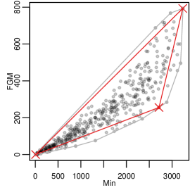
In order to illustrate archetypal analysis, we use a two-dimensional subset of the NBA player statistics from the season 2009/2010 which we analyze in Section 3.1: the two variables are total minutes played (Min) and field goals made (FGM) of 441 players, i.e., we investigate “the score efficiency”. Figure 1a shows the data set. The majority of players are in the range $[0,1000]$ of Min and $[0,200]$ of FGM. With increasing Min, the variance in FGM increases and the shape of the data set suggests the estimation of three archetypes. Figure 1b visualizes the $k=3$ archetypes solution (red), together with the data’s convex hull (gray). We see that this archetypes solution is a reasonable approximation of the convex hull (note that the archetypes do not have to be observed data points). Using this solution, the data points inside the archetypes solution are exactly approximated, the data points outside the archetypes solution are approximated with an error, as they are projected on the hull of the archetypes solution.

The three archetypes can be interpreted as follows. Concerning these two variables total minutes played (MIN) and field goals made (FGM), three types of extreme players are in the data set:

Archetype 1

is the natural “maximum” with high values in all variables ($\mbox{{Min}}=3234$, $\mbox{{FGM}}=793$); this archetype represents a type of “good” scorer.

Archetype 2

is the natural “minimum” with low values in all variables ($\mbox{{Min}}=7$, $\mbox{{FGM}}=0$); this archetype represents a type of “bad” scorer.

Archetype 3

is another extreme value with a high number of Min but a (relatively) low number of FGM ($\mbox{{Min}}=2713$, $\mbox{{FGM}}=256$); this archetype represents another type of “bad” scorer (i.e., an ineffective scorer).

Note that there is no archetype with a low number of Min and a high number of FGM; such an archetype would represent another type of “good” scorer (i.e., an effective scorer). An important aspect of the interpretation is, that it is conditioned on the given data; e.g., the number field goals made obviously is related to the position and tactical orientation of a player, but these information are not available in this illustrative data set and therefore cannot contribute to the interpretation of “good” and “bad” players.

(a)

(b)

Figure 2: (a) Visualization of the $\alpha$ coefficients using a ternary plot and (b) the data set in case of the $k=3$ archetypes solution. The red dots are the archetypes’ nearest players; dots colored with blue, orange, and green are players where Archetype 1, 2, and 3 contribute more than $0.8$.

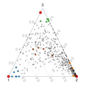
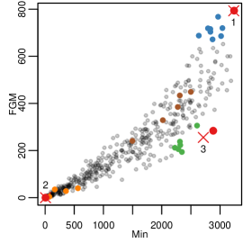
Having identified the possible extreme values within the given data set, the next step is to set the observations in relation to them. The $\alpha$ coefficients of the archetypal problem (Formula 1) define how much each archetype contributes to the approximation of each individual observation (as convex combination). This allows the assignment of the observations to their nearest archetypes and, consequently, the identification of the most archetypal observation(s). Figure 2 shows the corresponding ternary plot of the $\alpha$ coefficients for the above $k=3$ archetypes solution. The three players (red points) nearest to the respective archetypes (red crosses) are:

	Name	Team	Role	Min	FGM	$\alpha_{\cdot 1}$	$\alpha_{\cdot 2}$	$\alpha_{\cdot 3}$
Archetype 1	Kevin Durant	OKL	SF	3241	794	1.00	0.00	0.00
Archetype 2	Dwayne Jones	PHO	C	7	0	0.00	1.00	0.00
Archetype 3	Jason Kidd	DAL	PG	2883	284	0.06	0.00	0.94

Archetype 1 and 3 have well-defined nearest observations; Archetype 2, on the contrary, has a set of nearest observations and the concrete player identification should be considered as a “random” selection from the set of similar players.

We have identified Archetype 1 as the “good” archetype in this data setting—on this account, Kevin Durant can be considered as the best scorer. To find other good scorers, we look at the observations where Archetype 1 contributes more than $0.8$ (blue points):

Name	Team	Role	Min	FGM	$\alpha_{\cdot 1}$	$\alpha_{\cdot 2}$	$\alpha_{\cdot 3}$
Kevin Durant	OKL	SF	3241	794	1.00	0.00	0.00
Lebron James	CLE	SF	2967	768	0.95	0.05	0.00
Kobe Bryant	LAL	SG	2834	716	0.89	0.11	0.00
Dwyane Wade	MIA	SG	2793	719	0.89	0.11	0.00
Dirk Nowitzki	DAL	PF	3041	720	0.89	0.05	0.06
Amare Stoudemire	PHO	PF	2835	704	0.88	0.12	0.00
Carmelo Anthony	DEN	SF	2636	688	0.85	0.15	0.00
David Lee	NYK	C	3018	686	0.82	0.05	0.13
Derrick Rose	CHI	PG	2872	672	0.82	0.10	0.08

We equivalently proceed for the other two archetypes: Players where Archetype 3 contributes more than $0.8$ are Jason Kidd, Thabo Sefolosha, Earl Watson, Anthony Parker, Derek Fisher, Ron Artest, Marcus Camby (green points). Five randomly selected players where Archetype 2 contributes more than $0.8$ are Ryan Bowen, Sean Marks, Ian Mahinmi, Jamaal Magloire, Quinton Ross (orange points).

Observations toward the center of the data set are not approximated by one archetype alone, but each archetype contributes a significant fraction. The following five players, for example, are randomly selected from the data sets’ center (brown points):

Name	Team	Role	Min	FGM	$\alpha_{\cdot 1}$	$\alpha_{\cdot 2}$	$\alpha_{\cdot 3}$
Vince Carter	ORL	SG	2310	434	0.44	0.23	0.32
Anthony Morrow	GSW	SG	2019	329	0.28	0.31	0.40
C.j. Miles	UTA	SF	1497	241	0.21	0.49	0.31
Paul Millsap	UTA	PF	2275	385	0.35	0.23	0.42
Rodney Stuckey	DET	PG	2499	449	0.44	0.16	0.40

As we can see, based on the $\alpha$ coefficients of the players no assignments to one of the archetypes are possible.

Besides setting the observations in relation to their nearest archetype using the observations’ highest $\alpha$, the interpretation of all $\alpha$s of an observation is of interest as well. Suppose that, for example, the data set describes skill ratings of players, then the $\alpha$s can be interpreted as the players’ compositions of skills; see Section 3.2 for such an application of archetypal analysis.

3 Archetypal athletes

Archetypal analysis in general enables to compute data-driven extreme values and the corresponding observations’ (convex) combinations of all archetypes. In case of sports data this allows to identify and interpret archetypal athletes. Furthermore, all athletes are set in relation to the archetypal athletes and then can be “evaluated” according to them.

In this section we determine archetypal athletes for two popular sports and their representative leagues. Section 3.1 extends the illustrative two-dimensional example and computes archetypal basketball players with common statistics from the NBA season 2009/2010. Section 3.2 determines archetypal soccer players of the German Bundesliga, the English Premier League, the Italian Lega Serie A, and the Spanish La Liga using skill ratings (at the time of September 2011).

3.1 Archetypal basketball players

Figure 3: Parallel coordinates plot of the statistics of $441$ players from the NBA season 2009/2011.

Figure 4: Scree plot of the residual sum of squares for $1$ to $10$ archetypes.

Figure 5: Percentile plot of the four archetypal basketball players solution.

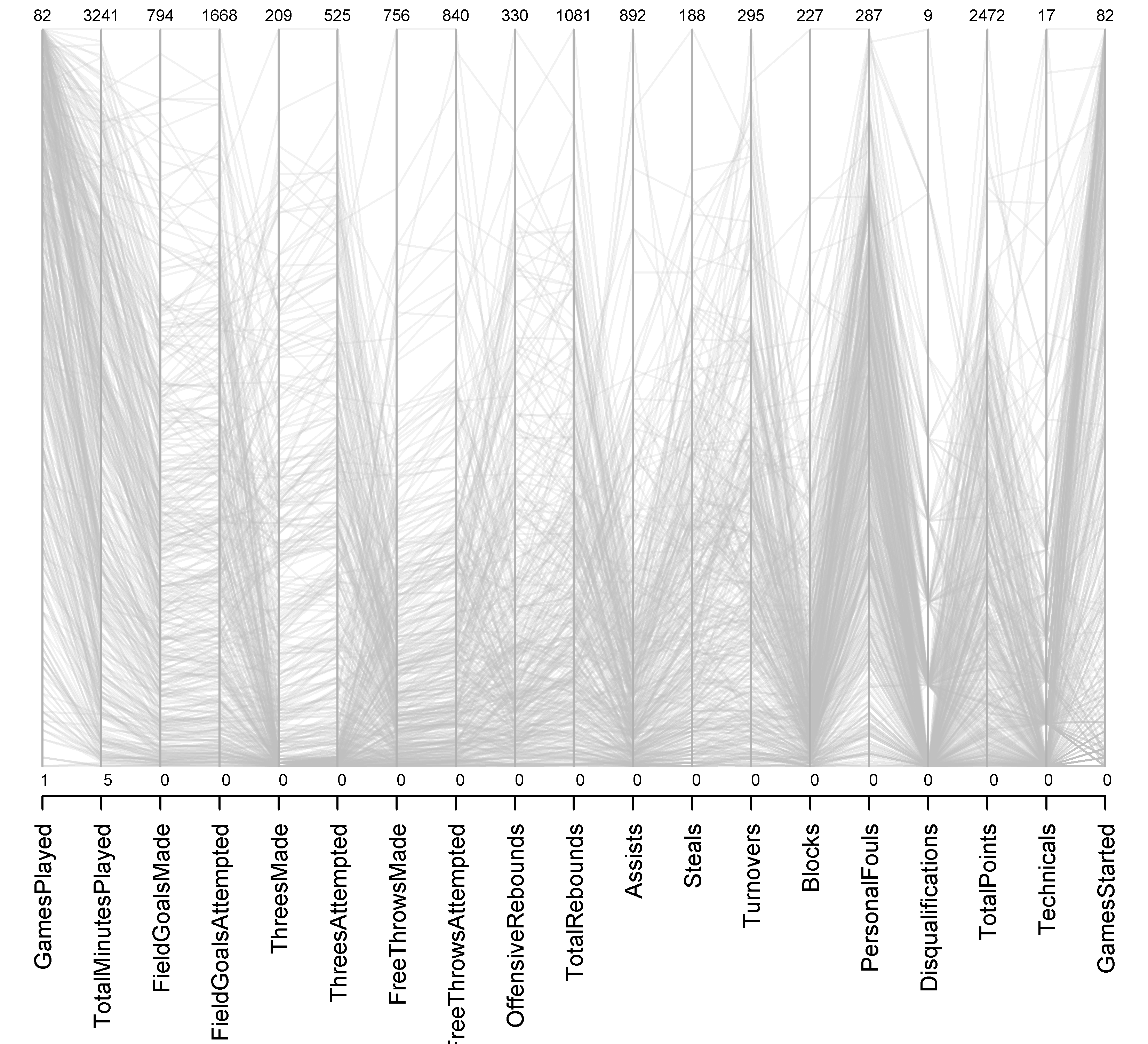
We determine the archetypal basketball players of the NBA season 2009/2010. Kubatko et al. (9) define basic variables used in what is now the mainstream of basketball statistics. Following their suggestion we use a data set provided by Steele (15) with $19$ statistics of $441$ players.

Figure 3 visualizes the data using a parallel coordinates plot. In comparison to the two-dimensional illustrative example no structure is easily observable; and there is, for example, no player which is the maximum over all statistics. We fit $k=1,\ldots,10$ archetypes; Figure 4 shows the corresponding scree plot: the first “elbow” is at $k=4$ ($RSS=0.04$), the second one at $k=8$ ($RSS=0.03$). The additional error reduction between $k=4$ and $k=8$ is marginal and we decide on $k=4$ archetypal basketball players.

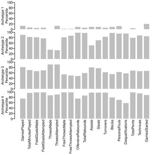
Figure 5 displays the percentile plots (i.e., the percentile value in an archetype as compared to the data) of the four archetypal basketball players available in the NBA season 2009/2010. The particular characteristics are:

Archetype 1

is the archetypal “benchwarmer” with few games played and therefore low values in all statistics.

Archetype 2

is the archetypal rebounder and defensive player with high values in the rebounds, blocks and foul-related statistics, and low values in the three-pointers.

Archetype 3

is the archetypal three-point shooter with high values in the three-pointer statistics and low values in the free throws and rebounds.

Archetype 4

is the archetypal offensive player with high values in all throw-related statistics and low values in foul-related statistics.

Archetype 1 represents a type of “bad” basketball player while all others represent different types of “good” players. The four basketball player nearest to one of the four archetypes are:

	Name	Team	Role	$\alpha_{\cdot 1}$	$\alpha_{\cdot 2}$	$\alpha_{\cdot 3}$	$\alpha_{\cdot 4}$
Archetype 1	Dwayne Jones	PHO	C	1.00	0.00	0.00	0.00
Archetype 2	Taj Gibson	CHI	SF	0.00	1.00	0.00	0.00
Archetype 3	Anthony Morrow	GSW	SG	0.00	0.00	0.96	0.04
Archetype 4	Kevin Durant	OKL	SF	0.00	0.00	0.00	1.00

On this account, Taj Gibson, Anthony Morrow, Kevin Durant can be considered as the best basketball players of the season 2009/2010 with respect to the characteristics of their corresponding archetypes. However, note that in case of Archetype 3 the player is not exactly the archetype. In order to find all good players, we look at the observations where one of the three “good” archetype contributes more than $0.95$:

Archetype	Name	Team	Role	$\alpha_{\cdot 1}$	$\alpha_{\cdot 2}$	$\alpha_{\cdot 3}$	$\alpha_{\cdot 4}$
Archetype 2	Taj Gibson	CHI	SF	0.00	1.00	0.00	0.00
	Andrew Bogut	MIL	C	0.00	1.00	0.00	0.00
	Samuel Dalembert	PHI	C	0.02	0.98	0.00	0.00
	Jason Thompson	SAC	PF	0.03	0.96	0.00	0.00
Archetype 3	Anthony Morrow	GSW	SG	0.00	0.00	0.96	0.04
	Steve Blake	LAC	PG	0.02	0.00	0.96	0.02
Archetype 4	Kevin Durant	OKL	SF	0.00	0.00	0.00	1.00
	Lebron James	CLE	SF	0.00	0.00	0.00	1.00
	Dwyane Wade	MIA	SG	0.00	0.00	0.00	1.00
	Kobe Bryant	LAL	SG	0.03	0.00	0.00	0.97

The equal coefficients, e.g. for the first two players in case of Archetype 2, occur due to rounding to two decimal places. The threshold $0.95$ is arbitrarily defined; this is, in fact, the only subjective decision one has to make when discussing the quality of athletes using archetypal analysis.

3.2 Archetypal soccer players

The skill ratings are from the PES Stats Database (12) (PSD), a community-based approach to create a database with accurate statistics and skill ratings for soccer players (originally for the video game “Pro Evolution Soccer” by Konami). The extracted data set consists of $25$ skills of $1658$ players (all positions—Defender, Midfielder, Forward—except Goalkeepers) from the German Bundesliga, the English Premier League, the Italian Serie A, and the Spanish La Liga. The skills are rated from 0 to 100 and describe different abilites of the players: physical abilities like balance, stamania, and top speed; ball skills like dribble, pass, and shot accuracy and speed; and general skills like attack and defence performance, technique, aggression, and teamwork. Note that we assume that the differences are interpretable, i.e., the ratings are on a ratio scale.

Figure 6: Parallel coordinates of the skill ratings of of $1658$ players from the German Bundesliga, the English Premier League, the Italian Serie A, and the Spanish La Liga.

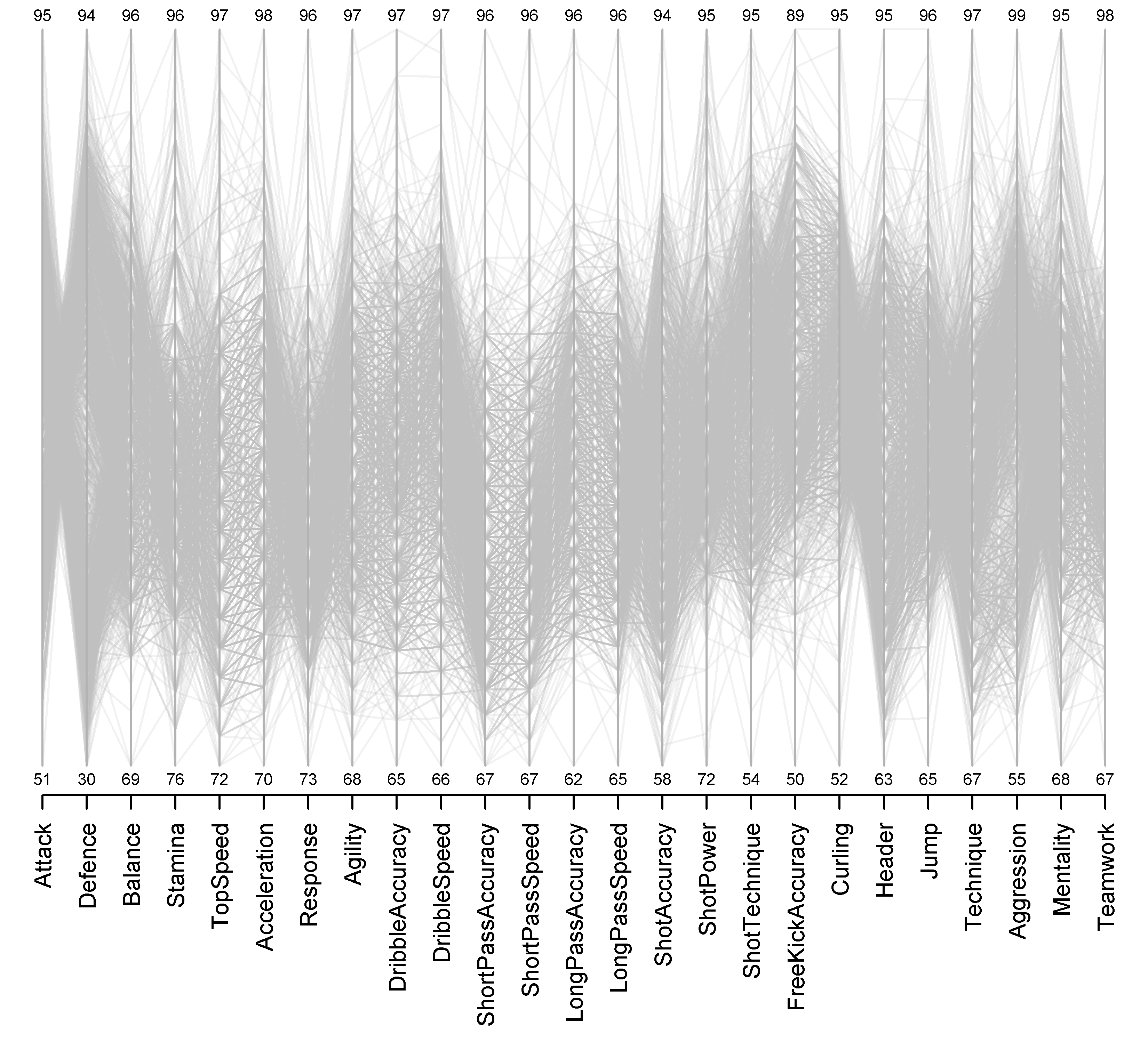
Figure 6 shows a parallel coordinates plot of the data set. Most skills range between 50 and 100; this is due to the fact that PSD describes soccer players of all hierarchy levels of a league system. Anyway, no real structure is visible in the data, and there are no players which are the maximum or the minimum over all skills. We decide to use $k=4$ archetypal soccer players; see the online supplement for the decision process (section on computational details on page Computational details).

Figure 7: Percentile plot of the four archetypal soccer players solution.

Figure 8: Parallel coordinates plot of $\alpha$ coefficients of the four archetypal soccer players solution with highlighted defenders (red).

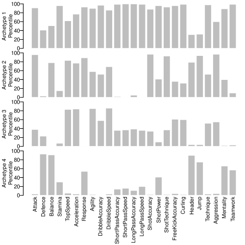
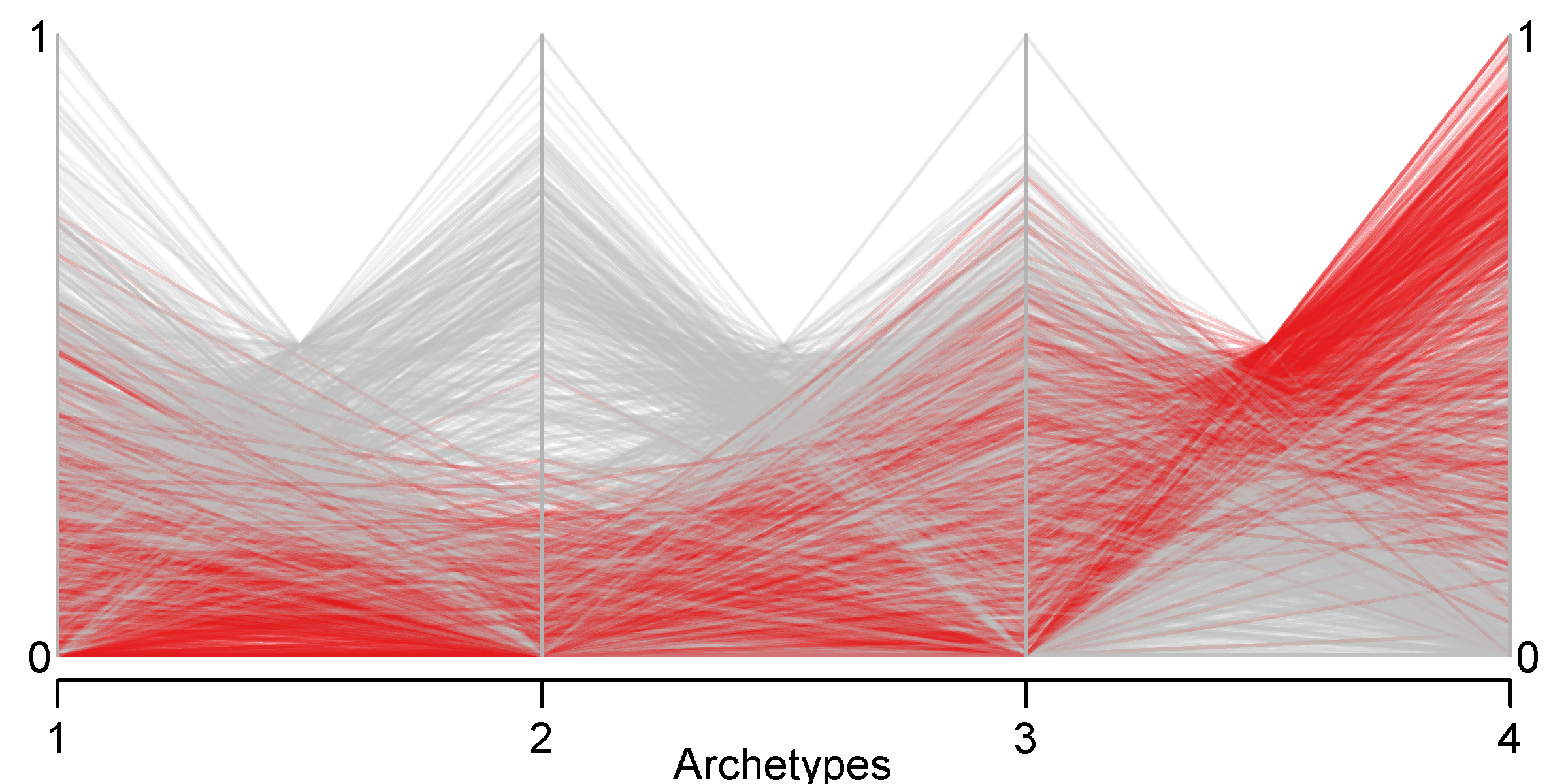
Figure 7 displays the percentile plots of the four archeypal soccer players. The particular characteristical skills are:

Archetype 1

is the archetypal offensive player with all skills high excpect the defense, balance, header, and jump.

Archetype 2

is the archetypal center forward with high skills in attack, shot, acceleration, header and jump, and low passing skills.

Archetype 3

is the archetypal weak soccer player with high skills in running, but low skills in most ball related skills.

Archetype 4

is the archetypal defender with high skills in defense, balance, header, and jump.

To verify this interpretation we look at the $\alpha$ coefficients in combination with the players’ position; Figure 8 exemplarily shows the parallel coordinates plot with the “Defender” position highlighted (red). As we can see, nearly all defenders have a high $\alpha$ coefficient for Archetype 4.

Now, in order to investigate the question of the best soccer player we have to make a (subjective) definition of “the best” in terms of the four archetypes. For us, the best player is a combination of Archetype 1 and Archetype 2 with Archetype 1 contributing more than Archetype 2 (according to the common sense that offensive players are match-winning). The following soccer players apply to the definition (orderd according to $\alpha_{\cdot 1}$):

Name	Club	$\alpha_{\cdot 1}$	$\alpha_{\cdot 2}$	$\alpha_{\cdot 3}$	$\alpha_{\cdot 4}$
Wayne Rooney	Manchester United FC	0.82	0.18	0.00	0.00
Leo Messi	FC Barcelona	0.79	0.21	0.00	0.00
Cristiano Ronaldo	Real Madrid CF	0.68	0.32	0.00	0.00
Antonio Di Natale	Udinese Calcio	0.67	0.33	0.00	0.00
Carlos Tivez	Manchester City FC	0.66	0.34	0.00	0.00
Diego Forlan	FC Internazionale Milano	0.64	0.36	0.00	0.00
Dimitar Berbatov	Manchester United FC	0.60	0.40	0.00	0.00
Adrian Mutu	AC Cesena	0.60	0.40	0.00	0.00
Zlatan Ibrahimovic	AC Milan	0.54	0.46	0.00	0.00
Luis Suarez	Liverpool FC	0.53	0.47	0.00	0.00
Mladen Petric	Hamburger SV	0.53	0.47	0.00	0.00
Xavi Hernandez	FC Barcelona	0.52	0.48	0.00	0.00
Didier Drogba	Chelsea FC	0.52	0.48	0.00	0.00
Giuseppe Rossi	Villarreal CF	0.51	0.49	0.00	0.00

Based on our definition and the given skill rating data set, Wayne Rooney is the best player, followed by Leo Messi and Cristiano Ronaldo.

4 Conclusion

The present paper applies the statistical method archetypal analysis to sports data. This enables to compute outstanding—positively and/or negatively—athletes, i.e., the archetypal athletes. Statements like “Dirk Nowitzki is the best basketball player. No, it’s Kevin Durant!” can be then discussed completely data-driven and with a well-defined and reproducible amount of subjectivity. The proposed way is (1) to estimate the archetypes, i.e., the archetypal athletes, then (2) to identify the athletes as different types of “good” and “bad” athletes, and finally (3) to set all athletes in relation to the archetypes (using the $\alpha$ coefficients). The two examples—basketball and soccer—shows that this is an appropriate approach; the estimated archetypal athletes definitely are consistent with the general opinion.

Computational details

All computations and graphics have been done using the statistical software R 2.13.1 (14), the archetypes package (4), and the SportsAnalytics package (5). R itself and all packages used are freely available under the terms of the General Public License from the Comprehensive R Archive Network at http://CRAN.R-project.org/.

Data sets and source codes for replicating our analyses are available in the SportsAnalytics package. An individual analysis is executed via (replace *** with nba-2d, nba and soccer):

R> demo("archeplayers-***", package = "SportsAnalytics")

The source code file for a demo is accessible via:

R> edit(file = system.file("demo", "archeplayers-***.R",
+                          package = "SportsAnalytics"))

Affiliation:
Manuel J. A. Eugster
Institut für Statistik
Ludwig-Maximilians-Universtität München
80530 Munich, Germany
E-mail: Manuel.Eugster@stat.uni-muenchen.de
Website: http://www.statistik.lmu.de/~eugster/

References

- Bauckhage and Thurau (2009) Christian Bauckhage and Christian Thurau. Making archetypal analysis practical. In Proceedings of the 31st DAGM Symposium on Pattern Recognition, pages 272–281, 2009. 10.1007/978-3-642-03798-6_28.
- Chan et al. (2003) Ben H. P. Chan, Daniel A. Mitchell, and Lawrence E. Cram. Archetypal analysis of galaxy spectra. Monthly Notice of the Royal Astronomical Society, 338:790–795, 2003. 10.1046/j.1365-8711.2003.06099.x.
- Cutler and Breiman (1994) Adele Cutler and Leo Breiman. Archetypal analysis. Technometrics, 36(4):338–347, 1994.
- Eugster (2010) Manuel J. A. Eugster. archetypes: Archetypal Analysis, 2010. URL http://cran.r-project.org/package=archetypes. R package version 2.0-2.
- Eugster (2011) Manuel J. A. Eugster. SportsAnalytics: Sports Analytics, 2011. URL http://cran.r-project.org/package=SportsAnalytics. R package version 0.1.
- Eugster and Leisch (2009) Manuel J. A. Eugster and Friedrich Leisch. From Spider-man to Hero – Archetypal analysis in R. Journal of Statistical Software, 30(8):1–23, 2009. URL http://www.jstatsoft.org/v30/i08.
- Eugster and Leisch (2011) Manuel J. A. Eugster and Friedrich Leisch. Weighted and robust archetypal analysis. Computational Statistics and Data Analysis, 55(3):1215–1225, 2011. 10.1016/j.csda.2010.10.017. Preprint available from http://epub.ub.uni-muenchen.de/11498/.
- Hastie et al. (2009) Trevor Hastie, Robert Tibshirani, and Jerome Friedman. The Elements of Statistical Learning: Data Mining, Inference, and Prediction. Springer-Verlag, second edition, 2009. ISBN 0387848576.
- Kubatko et al. (2007) Justin Kubatko, Dean Oliver, Kevin Pelton, and Dan T. Rosenbaum. A starting point for analyzing basketball statistics. Journal of Quantitative Analysis in Sports, 3:Article 1, 2007. 10.2202/1559-0410.1070.
- Li et al. (2003) Shan Li, Paul Wang, Jordan Louviere, and Richard Carson. Archetypal analysis: A new way to segment markets based on extreme individuals. In A Celebration of Ehrenberg and Bass: Marketing Knowledge, Discoveries and Contribution. Proceedings of the ANZMAC 2003 Conference, December 1-3, 2003, pages 1674–1679, 2003.
- McHale and Scarf (2005) Ian McHale and Phil Scarf. Ranking football players. Significance, 2:54–57, 2005. 10.1111/j.1740-9713.2005.00091.x.
- PES Stats Database (2011) PES Stats Database. PSD – PES Stats Database. Website, 2011. http://pesstatsdatabase.com/; visited on .
- Porzio et al. (2008) Giovanni C. Porzio, Giancarlo Ragozini, and Domenico Vistocco. On the use of archetypes as benchmarks. Applied Stochastic Models in Business and Industry, 24(5):419–437, 2008. 10.1002/asmb.v24:5.
- R Development Core Team (2011) R Development Core Team. R: A Language and Environment for Statistical Computing. R Foundation for Statistical Computing, Vienna, Austria, 2011. URL http://www.R-project.org/. ISBN 3-900051-07-0.
- Steele (2011) Doug Steele. Doug’s NBA & MLB statistics home page. Website, 2011. http://dougstats.com/; visited on .
- Thorn and Palmer (1984) John Thorn and Pete Palmer. The Hidden Game of Baseball. Doubleday, 1984. ISBN 0385182848.