Lévy flights on the half line

Reinaldo García-García reinaldo.garcia@cab.cnea.gov.ar Centro Atómico Bariloche, 8400 S. C. de Bariloche, Argentina    Alberto Rosso alberto.rosso@u-psud.fr Laboratoire de Physique Théorique et Modèles Statistiques, Université Paris Sud 11 and CNRS    Grégory Schehr gregory.schehr@th.u-psud.fr Laboratoire de Physique Théorique d’Orsay, Université Paris Sud 11 and CNRS
Abstract

We study the probability distribution function (pdf) of the position of a Lévy flight of index 0<α<20𝛼20<\alpha<2 in presence of an absorbing wall at the origin. The solution of the associated fractional Fokker-Planck equation can be constructed using a perturbation scheme around the Brownian solution (corresponding to α=2𝛼2\alpha=2), as an expansion in ϵ=2αitalic-ϵ2𝛼\epsilon=2-\alpha. We obtain an explicit analytical solution, exact at the first order in ϵitalic-ϵ\epsilon, which allows us to conjecture the precise asymptotic behavior of this pdf, including the first subleading corrections, for any α𝛼\alpha. Careful numerical simulations, as well as an exact computation for α=1𝛼1\alpha=1, confirm our conjecture.

I Introduction

Random walks are trajectories consisting of a collection of random steps. They are employed to model the stochastic activity observed in many fields such as physics, biology, quantitative finance or computer science. As such they have been widely studied by mathematicians SA54 ; feller ; hughes_book and physicists montroll_weiss ; bouchaud_georges ; klafter_review ; satya_leuven . One of the simplest example is given by a symmetric one dimensional random walker whose position, x(n)𝑥𝑛x(n), after n𝑛n steps evolves, for n1𝑛1n\geq 1, according to

x(n)=x(n1)+η(n),𝑥𝑛𝑥𝑛1𝜂𝑛\displaystyle x{(n)}=x{(n-1)}+\eta(n)\;, (1)

starting from x(0)=0𝑥00x(0)=0. Moreover we consider random steps independent and identically distributed, according to a probability distribution φ(η)𝜑𝜂\varphi(\eta): consequently the random walk is Markovian and homogeneous.

Despite being simple to define, most of the properties of a random walk remain difficult to determine analytically. However, when the number of steps is large, the random walk displays a ”universal” behavior and the statistics of the position x(n)𝑥𝑛x(n) becomes independent of most of the details of φ(η)𝜑𝜂\varphi(\eta). This asymptotic regime is the one we have more chance to characterize and it is often the one which is relevant for applications. In this limit, two cases should be distinguished. If φ(η)𝜑𝜂\varphi(\eta) is a narrow distribution the random walk exhibits a diffusive behavior, x(n)n1/2similar-to𝑥𝑛superscript𝑛12x(n)\sim n^{1/2} and only the second moment of the step distribution, η2φ(η)𝑑η=σ2superscriptsubscriptsuperscript𝜂2𝜑𝜂differential-d𝜂superscript𝜎2\int_{-\infty}^{\infty}\eta^{2}\varphi(\eta)d\eta=\sigma^{2}, affects the statistics of x(n)𝑥𝑛x(n). On the other hand if the random variables η(n)𝜂𝑛\eta(n)’s have a broad distribution, with a diverging second moment, i.e.

φ(η)c|η|1+α,|η|1,formulae-sequencesimilar-to𝜑𝜂𝑐superscript𝜂1𝛼much-greater-than𝜂1\displaystyle\varphi(\eta)\sim\frac{c}{|\eta|^{1+\alpha}}\;,\;|\eta|\gg 1\;, (2)

with 0<α<20𝛼20<\alpha<2, the random walk exhibits a super-diffusive behavior x(n)n1/αsimilar-to𝑥𝑛superscript𝑛1𝛼x(n)\sim n^{1/\alpha}. Such power law distributions (2) have been initially studied in the early sixties in economy pareto and finance mandelbrot and in the early eighties they started to proliferate in physics where they have found many applications ranging from disordered and glassy systems, super-diffusion in micellar systems, laser-cooling of cold atoms shlesinger_book , random matrices biroli , photons in hot atomic vapours mercadier etc… One striking feature of such processes is that their statistical behavior is governed by a few rare events, whose occurrence are thus governed by the tail of the distribution.

Also in this case, when the number of steps becomes large, we expect that the statistics of x(n)𝑥𝑛x(n) becomes independent of the details of φ(η)𝜑𝜂\varphi(\eta) except for the index α𝛼\alpha and the constant c𝑐c. In particular, in absence of boundaries, the central limit theorem ensures that the propagator, P(x,n)𝑃𝑥𝑛P(x,n), i.e. the probability to find the particle in x𝑥x after n𝑛n steps, converges to a stable distribution given by:

P(x,n)=1n1/αR(y),𝑃𝑥𝑛1superscript𝑛1𝛼𝑅𝑦\displaystyle P(x,n)=\frac{1}{n^{1/\alpha}}R\left(y\right)\;, (3)
R(y)eiky𝑑y=e|ak|α,superscriptsubscript𝑅𝑦superscript𝑒𝑖𝑘𝑦differential-d𝑦superscript𝑒superscript𝑎𝑘𝛼\displaystyle\int_{-\infty}^{\infty}R(y)e^{iky}\,dy=e^{-|ak|^{\alpha}}\;, (4)

where the parameter a𝑎a is related to the constant c𝑐c [see Eq. (8) below] and where we have introduced, from dimensional analysis, the rescaled variable

yxn1/α.𝑦𝑥superscript𝑛1𝛼\displaystyle y\equiv\frac{x}{n^{1/\alpha}}\;. (5)

Although the Fourier transform of R(y)𝑅𝑦R(y), its characteristic function, has a very simple expression (4), there is no simple closed form expression for R(y)𝑅𝑦R(y), except for α=1𝛼1\alpha=1 which corresponds to Cauchy distribution. It however admits the following asymptotic expansion, valid for any value of α𝛼\alpha hughes_book :

R(y)1π|y|k=1aαksin(αkπ2)Γ(αk+1)(1)k+1k!|y|αk.similar-to𝑅𝑦1𝜋𝑦superscriptsubscript𝑘1superscript𝑎𝛼𝑘𝛼𝑘𝜋2Γ𝛼𝑘1superscript1𝑘1𝑘superscript𝑦𝛼𝑘\displaystyle R(y)\sim\frac{1}{\pi|y|}\sum_{k=1}^{\infty}a^{\alpha k}\frac{\sin{\left(\frac{\alpha k\pi}{2}\right)}\Gamma(\alpha k+1)(-1)^{k+1}}{k!|y|^{\alpha k}}\;. (6)

One thus sees on this expression that R(y)𝑅𝑦R(y) inherits the power law tail of the step distribution (2). One can further show hughes_book ; feller that the amplitude itself is not renormalized such that to leading order

R(y)cy1+α+dy1+2α+𝒪(y13α),similar-to𝑅𝑦𝑐superscript𝑦1𝛼𝑑superscript𝑦12𝛼𝒪superscript𝑦13𝛼\displaystyle R(y)\sim\frac{c}{y^{1+\alpha}}+\frac{d}{y^{1+2\alpha}}+{\cal O}(y^{-{1-3\alpha}})\;, (7)

which fixes the value of a𝑎a

aα=πcsin(απ2)Γ(α+1),superscript𝑎𝛼𝜋𝑐𝛼𝜋2Γ𝛼1\displaystyle a^{\alpha}=\frac{\pi\,c}{\sin\left(\frac{\alpha\pi}{2}\right)\Gamma(\alpha+1)}\;, (8)

while d𝑑d can also be obtained explicitly from Eq. (6).

Although free Lévy flights are thus perfectly well understood, there are physical situations which actually involve Lévy flights in a confined geometry. An interesting example is the Lévy flight model which has been proposed davis_marshak to describe the transports of solar photons in cloudy atmosphere. These photons are eventually reflected back to space or absorbed by the ground, so their trajectories are bounded random walks. In such cloudy atmosphere, whose heigth is typically of the order of 101010 kms, the photons can be trapped in optically dense region (inside the clouds), travelling less than a meter between scatterings, while they can ”fly” many kilometers from cloud to cloud. It was shown experimentally that Lévy flights provide a reliable description of the photons transport in such situations pfeilsticker . It was shown, in addition, that the one-dimensional model is a reasonable approximation of the three-dimensional geometry davis_pfeilsticker . More recently, Lévy flights in confined geometry have also found applications in the context of random search problems jpa_stanley .

Obviously, when the walker is confined inside a domain, the central limit theorem does not apply, but the scaling analysis is still valid and the ”universal” behavior of the rescaled position y=x/n1/α𝑦𝑥superscript𝑛1𝛼y=x/n^{1/\alpha} is still expected. Computing the statistics of the rescaled variable y𝑦y in presence of confinement is in general possible for Brownian motion (α=2𝛼2\alpha=2) for which powerful analytical tools are available such as path-integral techniques yor_functional ; satya_functional . Unfortunately, for Lévy flights, analytical approaches are usually quite difficult. Recently a lot of papers advertised the possibility to write a Fractional Fokker-Planck equation for Lévy flight propagator klafter_review :

tP(x,t)=aαα|x|αP(x,t),P(x,t=0)=δ(x),formulae-sequence𝑡𝑃𝑥𝑡superscript𝑎𝛼superscript𝛼superscript𝑥𝛼𝑃𝑥𝑡𝑃𝑥𝑡0𝛿𝑥\displaystyle\frac{\partial}{\partial t}P(x,t)=a^{\alpha}\frac{\partial^{\alpha}}{\partial|x|^{\alpha}}P(x,t)\;,\;P(x,t=0)=\delta(x)\;, (9)

where the continuum time t𝑡t captures the large n𝑛n behavior of the random walk and the fractional operator, α|x|αsuperscript𝛼superscript𝑥𝛼\frac{\partial^{\alpha}}{\partial|x|^{\alpha}}, is the Riesz-Feller derivative of fractional order α>0𝛼0\alpha>0 IP99 ; SKM93 , which has an integral representation involving a singular kernel of power-law form. In absence of boundaries this equation can be simply written in Fourier space

tP~(k,t)=|ak|αP~(k,t),P~(k,t=0)=1,formulae-sequence𝑡~𝑃𝑘𝑡superscript𝑎𝑘𝛼~𝑃𝑘𝑡~𝑃𝑘𝑡01\displaystyle\frac{\partial}{\partial t}\tilde{P}(k,t)=-|a\,k|^{\alpha}\tilde{P}(k,t)\;,\>\tilde{P}(k,t=0)=1\;, (10)

and it is easy to check that the free propagator introduced in Eq. (3) is a solution of Eq. (10), (with the identification, tn1𝑡𝑛much-greater-than1t\to n\gg 1).

In presence of boundaries the translational invariance is broken and the Fourier representation becomes useless. For α=2𝛼2\alpha=2, when the fractional operator becomes the standard Laplacian, the method of images allows to express the propagator in presence of boundaries as a linear combination of free propagators. Unfortunately we will see that these techniques can not be applied, for α<2𝛼2\alpha<2 ZK95 ; metzler_images . More generally, if translational invariance is lost, the fractional Fokker-Planck equation in Eq. (9), becomes a difficult integro-differential equation with non-local boundary conditions. One could conclude that the Fokker-Planck formalism is of little help for Lévy flights. However, following a recent work by Zoia, Rosso and Kardar ZRK07 , we show that Eq. (9 ) can be studied also in presence of boundaries using a perturbation theory where the small parameter ϵ1much-less-thanitalic-ϵ1\epsilon\ll 1 is α=2ϵ𝛼2italic-ϵ\alpha=2-\epsilon. At variance with the method of Ref. ZRK07 we perform this perturbation theory directly in the continuum limit without resorting to a discretization (in space) of the trajectories. The calculations turn out to be somewhat simpler in this continuum setting.
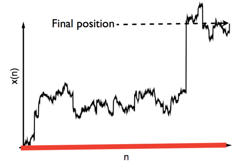
Refer to caption
Figure 1: Trajectory of a random walker with an absorbing boundary condition at the origin. P+(x,t)subscript𝑃𝑥𝑡P_{+}(x,t), computed perturbatively in Eq. (94), is the probability density function of the position of such a random walker at time t𝑡t.

For concreteness we will study in detail the case where there is an absorbing wall in x=0𝑥0x=0 as depicted in Fig. 1: we thus consider only the paths that remain positive up to the nthsuperscript𝑛thn^{\rm th} step. In the limit of large n𝑛n the probability density function to find the particle in x𝑥x after n𝑛n time steps also takes the scaling form, as in Eq. (3):

P+(x,n)=1n1/αR+(y).subscript𝑃𝑥𝑛1superscript𝑛1𝛼subscript𝑅𝑦\displaystyle P_{+}(x,n)=\frac{1}{n^{1/\alpha}}R_{+}\left(y\right)\;. (11)

We emphasize that R+(y)subscript𝑅𝑦R_{+}(y), being a probability density function, is normalized, i.e. 0R+(y)𝑑y=1superscriptsubscript0subscript𝑅𝑦differential-d𝑦1\int_{0}^{\infty}R_{+}(y)\,dy=1, while, in Ref. ZK95 , Zumofen and Klafter studied a similar quantity, which is however not normalized (see also Ref. ivanov ). In particular, they were able to show that the small argument behavior of R+(y)subscript𝑅𝑦R_{+}(y) is given by ZK95 ; zoia_semi_inf

R+(y)yα/2,similar-tosubscript𝑅𝑦superscript𝑦𝛼2\displaystyle R_{+}(y)\sim y^{\alpha/2}\;, (12)

in contrast with the method of images that would predict R+(y)ysimilar-tosubscript𝑅𝑦𝑦R_{+}(y)\sim y. Our perturbative approach allows us to conjecture the exact behavior of the tail of R+(y)subscript𝑅𝑦R_{+}(y), which controls the statistics of rare events :

R+(y)=c+y1+α+{d+y2+α+o(y2α), 2>α>1,d+y1+2α+o(y12α), 1>α>0.subscript𝑅𝑦subscript𝑐superscript𝑦1𝛼casesotherwisesubscript𝑑superscript𝑦2𝛼𝑜superscript𝑦2𝛼2𝛼1otherwiseotherwiseotherwisesubscript𝑑superscript𝑦12𝛼𝑜superscript𝑦12𝛼1𝛼0\displaystyle R_{+}(y)=\frac{c_{+}}{y^{1+\alpha}}\;+\;\begin{cases}&\frac{d_{+}}{y^{2+\alpha}}+o(y^{-2-\alpha})\;,\;2>\alpha>1\;,\\ &\\ &\frac{d_{+}}{y^{1+2\alpha}}+o(y^{-1-2\alpha})\;,\;1>\alpha>0\;.\end{cases} (13)

To our knowledge, only the exponent of the leading term R+(y)y1αproportional-tosubscript𝑅𝑦superscript𝑦1𝛼R_{+}(y)\propto y^{-1-\alpha}, was known from Ref. ZK95 . Here we obtain the exact result for the amplitude c+subscript𝑐c_{+}

c+=2c,subscript𝑐2𝑐\displaystyle c_{+}=2c\;, (14)

where c𝑐c is the amplitude of the tail of the jump distribution (2). In addition, the first sub-leading corrections in Eq. (13), by comparison to the free case (7), also bear the fingerprints of the absorbing wall. These results (13) are first obtained analytically for α𝛼\alpha close to 222, i.e. α=2ϵ𝛼2italic-ϵ\alpha=2-\epsilon, using a perturbation theory to first order in ϵitalic-ϵ\epsilon. We also obtain this behavior for α=1𝛼1\alpha=1, albeit with logarithmic corrections for the subleading term, for which an exact calculation can be done. We then demonstrate this behavior using thorough numerical simulations.

The paper is organized as follows. In Section II we present the general framework of the perturbation scheme. We first illustrate it on the simplest example of the free propagator in Section II A, and then in Section II B we study the case with an absorbing boundary at the origin. The discussion of the results is left in Section II C. Section III contains the results of our numerical simulations and our conclusions are in section IV. The Appendices A, B, C contain some technical details.

II Perturbation scheme

In this section, we set a=1𝑎1a=1 for simplicity and without loss of generality, and write the Fractional Fokker-Planck equation (9) in the familiar Schrödinger form

tP(x,x0,t)=P(x,x0,t),subscript𝑡𝑃𝑥subscript𝑥0𝑡𝑃𝑥subscript𝑥0𝑡\displaystyle\partial_{t}P(x,x_{0},t)={\cal H}P(x,x_{0},t)\;, (15)
P(x,x0,t=0)=δ(xx0),𝑃𝑥subscript𝑥0𝑡0𝛿𝑥subscript𝑥0\displaystyle P(x,x_{0},t=0)=\delta(x-x_{0})\;, (16)

where the propagator P(x,x0,t=0)𝑃𝑥subscript𝑥0𝑡0P(x,x_{0},t=0) represents the probability density to find a particle in the interval [x,x+dx]𝑥𝑥𝑑𝑥[x,x+dx] at time t𝑡t, knowing that the particle was in x0subscript𝑥0x_{0} at time 00 and the operator {\cal H} is the fractional operator of index α𝛼\alpha. In Quantum Mechanics Eq. (15) corresponds to the Schrödinger equation of the element (x,x0)𝑥subscript𝑥0(x,x_{0}) of the density matrix P𝑃P at the temperature 1/t1𝑡1/t. The general solution of Eq. (15) reads

P(x,x0,t)=𝑑qψq(x0)ψq(x)eE(q)t,𝑃𝑥subscript𝑥0𝑡differential-d𝑞superscriptsubscript𝜓𝑞subscript𝑥0subscript𝜓𝑞𝑥superscript𝑒𝐸𝑞𝑡P(x,x_{0},t)=\int dq\,\psi_{q}^{*}(x_{0})\psi_{q}(x)e^{E(q)t}\;, (17)

where E(q)𝐸𝑞E(q) are the eigenvalues and ψq(x)subscript𝜓𝑞𝑥\psi_{q}(x) the associated eigenfunctions of the operator {\cal H}. They are solutions of the eigenvalue problem, ψq(x)=E(q)ψq(x)subscript𝜓𝑞𝑥𝐸𝑞subscript𝜓𝑞𝑥{\cal H}\psi_{q}(x)=E(q)\psi_{q}(x), with the appropriate boundary conditions and satisfy the orthonormality and closure relations:

ψq(x)ψq(x)𝑑x=δ(qq),subscript𝜓𝑞𝑥superscriptsubscript𝜓superscript𝑞𝑥differential-d𝑥𝛿𝑞superscript𝑞\displaystyle\int\psi_{q}(x)\psi_{q^{\prime}}^{*}(x)dx=\delta(q-q^{\prime})\;, (18)
ψq(x)ψq(x)𝑑q=δ(xx).subscript𝜓𝑞𝑥superscriptsubscript𝜓𝑞superscript𝑥differential-d𝑞𝛿𝑥superscript𝑥\displaystyle\int\psi_{q}(x)\psi_{q}^{*}(x^{\prime})dq=\delta(x-x^{\prime})\;. (19)

Please note that the domain of integration over x𝑥x depend on the boundary condition and the integration over q𝑞q is meant over the all spectrum. If the spectrum is discrete the integral is replaced by a discrete sum.

The eigenvalue problem of the operator {\cal H} is in general very difficult and the solution is known only in the absence of boundaries where the eigenfunctions are simple plane waves. The case α=2𝛼2\alpha=2 corresponds to the standard Laplacian for which a lot of results are known. In particular the spectrum can be exactly solved in one dimension. A possible strategy to gain insights on the behavior of a Lévy flights in presence of boundaries is to use the perturbation scheme around the well studied α=2𝛼2\alpha=2 case. For α=2ϵ𝛼2italic-ϵ\alpha=2-\epsilon the operator {\cal H} and the propagator can be expanded in powers of ϵitalic-ϵ\epsilon,

P(x,x0,t)=P(0)(x,x0,t)ϵP(1)(x,x0,t)+𝒪(ϵ2)𝑃𝑥subscript𝑥0𝑡superscript𝑃0𝑥subscript𝑥0𝑡italic-ϵsuperscript𝑃1𝑥subscript𝑥0𝑡𝒪superscriptitalic-ϵ2\displaystyle P(x,x_{0},t)=P^{(0)}(x,x_{0},t)-\epsilon P^{(1)}(x,x_{0},t)+{\cal O}(\epsilon^{2})\;
=0ϵ1+O(ϵ2),subscript0italic-ϵsubscript1𝑂superscriptitalic-ϵ2\displaystyle{\cal H}={\cal H}_{0}-\epsilon{\cal H}_{1}+O(\epsilon^{2})\;, (20)

where P(0)(x,x0,t)superscript𝑃0𝑥subscript𝑥0𝑡P^{(0)}(x,x_{0},t) is the propagator associated to 0=x2subscript0superscriptsubscript𝑥2{\cal H}_{0}=\partial_{x}^{2}, with the prescribed boundary conditions. The expression of the first correction P(1)(x,x0,t)superscript𝑃1𝑥subscript𝑥0𝑡P^{(1)}(x,x_{0},t) in Eq. (II) is well known from Quantum Mechanics and it is re-derived in Appendix A. It reads, writing P(1)P(1)(x,x0,t)superscript𝑃1superscript𝑃1𝑥subscript𝑥0𝑡P^{(1)}\equiv P^{(1)}(x,x_{0},t):

P(1)=qqψq(x)ψq(x0)eE(q)teE(q)tE(q)E(q)q|1|q,superscript𝑃1subscript𝑞subscriptsuperscript𝑞subscript𝜓𝑞𝑥superscriptsubscript𝜓superscript𝑞subscript𝑥0superscript𝑒𝐸𝑞𝑡superscript𝑒𝐸superscript𝑞𝑡𝐸superscript𝑞𝐸𝑞quantum-operator-product𝑞subscript1superscript𝑞P^{(1)}=\int_{q}\int_{q^{\prime}}\psi_{q}(x)\psi_{q^{\prime}}^{*}(x_{0})\frac{e^{E(q)t}-e^{E(q^{\prime})t}}{E(q^{\prime})-E(q)}\langle q|{\cal H}_{1}|q^{\prime}\rangle, (21)

where we use the notation q𝑑qsubscript𝑞differential-d𝑞\int_{q}\equiv\int dq and where it is understood here that ψq(x)subscript𝜓𝑞𝑥\psi_{q}(x) are the eigenvectors and E(q)𝐸𝑞E(q) the corresponding eigenvalues of 0subscript0{\cal H}_{0} and for the matrix elements q|1|qquantum-operator-product𝑞subscript1superscript𝑞\langle q|{\cal H}_{1}|q^{\prime}\rangle we use the bra-ket notation, borrowed from Quantum Mechanics with x|q=ψq(x)inner-product𝑥𝑞subscript𝜓𝑞𝑥\langle x|q\rangle=\psi_{q}(x). This formula (21) is the cornerstone of the perturbation approach presented here.

II.1 Absence of boundaries

We first illustrate this perturbative approach by computing the first order correction to the Brownian propagator in absence of boundaries, i. e. the Gaussian propagator, when α=2ϵ𝛼2italic-ϵ\alpha=2-\epsilon and x0=0subscript𝑥00x_{0}=0. In this simple case the eigenvalue problem of 0=x2subscript0superscriptsubscript𝑥2{\cal H}_{0}=\partial_{x}^{2} gives:

ψq(x)=12πeiqx,E(q)=q2,<q<.formulae-sequencesubscript𝜓𝑞𝑥12𝜋superscript𝑒𝑖𝑞𝑥formulae-sequence𝐸𝑞superscript𝑞2𝑞\psi_{q}(x)=\frac{1}{\sqrt{2\pi}}e^{iqx},\;E(q)=-q^{2},\;-\infty<q<\infty. (22)

Using that k2ϵ=k2ϵk2log|k|+𝒪(ϵ2)superscript𝑘2italic-ϵsuperscript𝑘2italic-ϵsuperscript𝑘2𝑘𝒪superscriptitalic-ϵ2k^{2-\epsilon}=k^{2}-\epsilon\,k^{2}\log|k|+{\cal O}(\epsilon^{2}), the matrix element q|1|qquantum-operator-product𝑞subscript1superscript𝑞\langle q|{\cal H}_{1}|q^{\prime}\rangle can be explicitly computed:

q|1|q=𝑑x1𝑑x2dk2πψq(x1)ψq(x2)quantum-operator-product𝑞subscript1superscript𝑞triple-integraldifferential-dsubscript𝑥1differential-dsubscript𝑥2𝑑𝑘2𝜋superscriptsubscript𝜓𝑞subscript𝑥1subscript𝜓superscript𝑞subscript𝑥2\displaystyle\langle q|{\cal H}_{1}|q^{\prime}\rangle=\iiint dx_{1}\,dx_{2}\,\frac{dk}{2\pi}\psi_{q}^{*}(x_{1})\psi_{q^{\prime}}(x_{2})
×k2log|k|eik(x1x2)=δ(qq)q2log|q|,\displaystyle\times\,k^{2}\log|k|e^{ik(x_{1}-x_{2})}=\delta(q-q^{\prime})q^{2}\log|q|, (23)

where the integral over x1,x2,ksubscript𝑥1subscript𝑥2𝑘x_{1},x_{2},k is performed over the whole real axis. Note that, thanks to the oscillating term eik(x1x2)superscript𝑒𝑖𝑘subscript𝑥1subscript𝑥2e^{ik(x_{1}-x_{2})}, the integral over k𝑘k in (II.1) is dominated by the small values of k𝑘k where one can safely expand k2ϵsuperscript𝑘2italic-ϵk^{2-\epsilon} in powers of ϵitalic-ϵ\epsilon. From Eq. (21) one obtains:

P(1)(x,t)=t0dqπcosqxq2logqeq2t.superscript𝑃1𝑥𝑡𝑡superscriptsubscript0𝑑𝑞𝜋𝑞𝑥superscript𝑞2𝑞superscript𝑒superscript𝑞2𝑡P^{(1)}(x,t)=-t\,\int_{0}^{\infty}\,\frac{dq}{\pi}\,\cos{qx}\,q^{2}\,\log q\,e^{-q^{2}t}. (24)

Using k=qt𝑘𝑞𝑡k=q\sqrt{t} and the scaling variable z=x/t𝑧𝑥𝑡z=x/\sqrt{t}, Eq. (24) can be recast in a simpler form

tP(1)(x,t)=RA(z)+RB(z)logt,𝑡superscript𝑃1𝑥𝑡subscript𝑅𝐴𝑧subscript𝑅𝐵𝑧𝑡\displaystyle\sqrt{t}\,P^{(1)}(x,t)=R_{A}(z)+R_{B}(z)\log t\;, (25)
RA(z)=0dkπcoskzk2logkek2,subscript𝑅𝐴𝑧superscriptsubscript0𝑑𝑘𝜋𝑘𝑧superscript𝑘2𝑘superscript𝑒superscript𝑘2\displaystyle R_{A}(z)=-\int_{0}^{\infty}\,\frac{dk}{\pi}\,\cos{kz}\,k^{2}\,\log k\,e^{-k^{2}}\;, (26)
RB(z)=0dk2πcoskzk2ek2.subscript𝑅𝐵𝑧superscriptsubscript0𝑑𝑘2𝜋𝑘𝑧superscript𝑘2superscript𝑒superscript𝑘2\displaystyle R_{B}(z)=\int_{0}^{\infty}\,\frac{dk}{2\pi}\,\cos{kz}\,k^{2}\,e^{-k^{2}}\;. (27)

From scaling argument one expects (3)

P(x,t)=1t1/αR(xt1/α),𝑃𝑥𝑡1superscript𝑡1𝛼𝑅𝑥superscript𝑡1𝛼\displaystyle P(x,t)=\frac{1}{t^{1/\alpha}}R\left(\frac{x}{t^{1/\alpha}}\right)\;, (28)

and a general issue of these perturbative computations is that for α=2𝛼2\alpha=2 the natural scaling variable is z=x/t𝑧𝑥𝑡z=x/\sqrt{t}, while for α=2ϵ𝛼2italic-ϵ\alpha=2-\epsilon the correct scaling variable is y=x/t12ϵ𝑦𝑥superscript𝑡12italic-ϵy=x/t^{\frac{1}{2-\epsilon}}, which also admits a perturbative expansion. For this reason our final result should be recast in terms of y𝑦y, in order to identify the perturbative expansion of the scaling function R(y)𝑅𝑦R(y) in Eq. (28) as

R(y)=R(0)(y)ϵR(1)(y)+𝒪(ϵ2),𝑅𝑦superscript𝑅0𝑦italic-ϵsuperscript𝑅1𝑦𝒪superscriptitalic-ϵ2\displaystyle R(y)=R^{(0)}(y)-\epsilon R^{(1)}(y)+{\cal O}(\epsilon^{2})\;, (29)

where R(0)(y)superscript𝑅0𝑦R^{(0)}(y) is the Gaussian propagator given by

R(0)(y)=12πey2/4.superscript𝑅0𝑦12𝜋superscript𝑒superscript𝑦24\displaystyle R^{(0)}(y)=\frac{1}{2\sqrt{\pi}}e^{-y^{2}/4}\;. (30)

This can be done if in the equation t1/αP(x,t)=R(y)superscript𝑡1𝛼𝑃𝑥𝑡𝑅𝑦t^{1/\alpha}P(x,t)=R(y) we expand at the first order in ϵitalic-ϵ\epsilon both t1/αt+ϵ4tlogtsimilar-tosuperscript𝑡1𝛼𝑡italic-ϵ4𝑡𝑡t^{1/\alpha}\sim\sqrt{t}+\frac{\epsilon}{4}\sqrt{t}\log t and yz+14ϵzlogtsimilar-to𝑦𝑧14italic-ϵ𝑧𝑡y\sim z+\frac{1}{4}\epsilon z\log t. After some simple algebra we can write

tP(1)(x,t)=R(1)(z)+ϵ4logt(1+zz)R(0)(z).𝑡superscript𝑃1𝑥𝑡superscript𝑅1𝑧italic-ϵ4𝑡1𝑧subscript𝑧superscript𝑅0𝑧\sqrt{t}P^{(1)}(x,t)=R^{(1)}(z)+\frac{\epsilon}{4}\log t\left(1+z\partial_{z}\right)R^{(0)}(z)\;. (31)

Comparing with Eq. (25) we identify 4RB(z)=R(0)(z)+zzR(0)(z)4subscript𝑅𝐵𝑧superscript𝑅0𝑧𝑧subscript𝑧superscript𝑅0𝑧4R_{B}(z)=R^{(0)}(z)+z\partial_{z}R^{(0)}(z) so that we conclude that R(1)(y)superscript𝑅1𝑦R^{(1)}(y) in Eq. (29) is given by:

R(1)(y)=0dkπcoskyk2logkek2.superscript𝑅1𝑦superscriptsubscript0𝑑𝑘𝜋𝑘𝑦superscript𝑘2𝑘superscript𝑒superscript𝑘2\displaystyle R^{(1)}(y)=-\int_{0}^{\infty}\,\frac{dk}{\pi}\,\cos{ky}\,k^{2}\,\log k\,e^{-k^{2}}\;. (32)

By performing an asymptotic analysis of Eq. (32) for large y𝑦y one finds a series expansion of R(y)𝑅𝑦R(y) given in Eq. (29) which converges nowhere but exists as a formal power series:

R(y)ϵk=1(2k)!2(k1)!1y2k+1ϵ(1y3+12y5+180y7+).similar-to𝑅𝑦italic-ϵsuperscriptsubscript𝑘12𝑘2𝑘11superscript𝑦2𝑘1similar-toitalic-ϵ1superscript𝑦312superscript𝑦5180superscript𝑦7R(y)\sim\epsilon\sum_{k=1}^{\infty}\frac{(2k)!}{2(k-1)!}\frac{1}{y^{2k+1}}\sim\epsilon\left(\frac{1}{y^{3}}+\frac{12}{y^{5}}+\frac{180}{y^{7}}+\ldots\right).

This result in in perfect agreement with the expansion given in Eq. (6) for α=2ϵ𝛼2italic-ϵ\alpha=2-\epsilon.

II.2 Propagator in presence of an absorbing boundary at x=0𝑥0x=0

We consider now G+(x,x0,t)dxsubscript𝐺𝑥subscript𝑥0𝑡𝑑𝑥G_{+}(x,x_{0},t)\,dx, the probability to find a particle in the interval [x,x+dx]𝑥𝑥𝑑𝑥[x,x+dx] at time t𝑡t, knowing that the particle was in x0subscript𝑥0x_{0} at time 00 and given that it stayed positive up to time t𝑡t (see Fig. 1). At variance with the free propagator, the integral over x𝑥x of G+(x,x0,t)subscript𝐺𝑥subscript𝑥0𝑡G_{+}(x,x_{0},t) is smaller than one and gives the fraction of surviving walker up to time t𝑡t (i.e. the survival probability). In the geometry defined by Eq. (1) the initial position of the discrete random walk is x0=0subscript𝑥00x_{0}=0. Here we are considering a process which is continuous in time and this initial condition x0=0subscript𝑥00x_{0}=0, together with the presence of an absorbing boundary at the origin is ill-defined. Indeed, it is well known that if the continuous time walker crosses zero once it will re-cross zero infinitely many times immediately after the first crossing. Therefore, it is impossible to enforce the constraint x0=0subscript𝑥00x_{0}=0 and simultaneously forcing the position of the continuous time walker to be strictly positive immediately after. Therefore we set x0>0subscript𝑥00x_{0}>0 and small in order to regularize the continuous time process and we will take the limit x00subscript𝑥00x_{0}\to 0 at the end of the calculation. Our final result corresponds to the geometry of the Eq. (1) in the limit of a large number of steps.

It is useful to express G+(x,x0,t)subscript𝐺𝑥subscript𝑥0𝑡G_{+}(x,x_{0},t) in terms of rescaled variables as in Eq. (5):

G+(x,x0,t)=1t1/αZ(y,y0),subscript𝐺𝑥subscript𝑥0𝑡1superscript𝑡1𝛼𝑍𝑦subscript𝑦0\displaystyle G_{+}(x,x_{0},t)=\frac{1}{t^{1/\alpha}}Z(y,y_{0}), (33)

The scaling function Z(y,y0)𝑍𝑦subscript𝑦0Z(y,y_{0}) depends explicitly on α𝛼\alpha and we compute it here in perturbation theory for ϵ=2α1italic-ϵ2𝛼much-less-than1\epsilon=2-\alpha\ll~{}1:

Z(y,y0)=Z(0)(y,y0)ϵZ(1)(y,y0)+𝒪(ϵ2).𝑍𝑦subscript𝑦0superscript𝑍0𝑦subscript𝑦0italic-ϵsuperscript𝑍1𝑦subscript𝑦0𝒪superscriptitalic-ϵ2\displaystyle Z(y,y_{0})=Z^{(0)}(y,y_{0})-\epsilon\,Z^{(1)}(y,y_{0})+{\cal O}(\epsilon^{2})\>. (34)

In presence of an absorbing boundary at the origin, the action of the fractional operator can be written as

0𝑑xψq(x)dk2π(|k|α)eik(xx)=E(q)ψq(x),superscriptsubscript0differential-dsuperscript𝑥subscript𝜓𝑞superscript𝑥superscriptsubscript𝑑𝑘2𝜋superscript𝑘𝛼superscript𝑒𝑖𝑘𝑥superscript𝑥𝐸𝑞subscript𝜓𝑞𝑥\int_{0}^{\infty}\,dx^{\prime}\psi_{q}(x^{\prime})\int_{-\infty}^{\infty}\,\frac{dk}{2\pi}(-|k|^{\alpha})\,e^{ik(x-x^{\prime})}=E(q)\psi_{q}(x), (35)

and the solution is known only for α=2𝛼2\alpha=2:

ψq(x)=θ(x)2πsin(qx),E(q)=q2,q>0,formulae-sequencesubscript𝜓𝑞𝑥𝜃𝑥2𝜋𝑞𝑥formulae-sequence𝐸𝑞superscript𝑞2𝑞0\psi_{q}(x)=\theta(x)\sqrt{\frac{2}{\pi}}\sin(qx)\;,\;E(q)=-q^{2}\;,\;q>0\;, (36)

where θ(x)𝜃𝑥\theta(x) is the Heaviside function: θ(x)=1𝜃𝑥1\theta(x)=1 if x0𝑥0x\geq 0 and θ(x)=0𝜃𝑥0\theta(x)=0 if x<0𝑥0x<0. At zeroth order in ϵitalic-ϵ\epsilon, the scaling function Z(0)(y,y0)superscript𝑍0𝑦subscript𝑦0Z^{(0)}(y,y_{0}) can be computed from Eq. (17) with ψq(x)subscript𝜓𝑞𝑥\psi_{q}(x) given in Eq. (36). Using the identity 2sin(ky)sin(ky0)=cos[k(yy0)]cos[k(y+y0)]2𝑘𝑦𝑘subscript𝑦0𝑘𝑦subscript𝑦0𝑘𝑦subscript𝑦02\sin(ky)\sin(ky_{0})=\cos{[k(y-y_{0})]}-\cos{[k(y+y_{0})]} one obtains:

Z(0)(y,y0)superscript𝑍0𝑦subscript𝑦0\displaystyle Z^{(0)}(y,y_{0}) =\displaystyle= θ(y)θ(y0)0dkπek2(cos[k(yy0)]\displaystyle\theta(y)\theta(y_{0})\int_{0}^{\infty}\frac{dk}{\pi}e^{-k^{2}}\big{(}\cos[k(y-y_{0})] (37)
cos[k(y+y0)]).\displaystyle-\cos[k(y+y_{0})]\Big{)}\;.

Let us note that the same result can be straightforwardly obtained using the method of images:

Z(0)(y,y0)=θ(y)θ(y0)[R(0)(yy0)R(0)(y+y0)].superscript𝑍0𝑦subscript𝑦0𝜃𝑦𝜃subscript𝑦0delimited-[]superscript𝑅0𝑦subscript𝑦0superscript𝑅0𝑦subscript𝑦0Z^{(0)}(y,y_{0})=\theta(y)\theta(y_{0})[R^{(0)}(y-y_{0})-R^{(0)}(y+y_{0})]\;. (38)

At the first order in ϵitalic-ϵ\epsilon we first compute the matrix element q|1|qquantum-operator-product𝑞subscript1superscript𝑞\langle q|{\cal H}_{1}|q^{\prime}\rangle which has the form given in Eq. (II.1) with the prescription that the integrals over x1subscript𝑥1x_{1} and x2subscript𝑥2x_{2} are performed over the interval (0,)0(0,\infty) and ψq(x)subscript𝜓𝑞𝑥\psi_{q}(x) are the eigenvectors given in Eq. (36). The integrals over x1subscript𝑥1x_{1} and x2subscript𝑥2x_{2} need to be regularized to be well defined and this can be done via the identity:

limϵ00dxπeikxϵxsin(qx)=PVqπ(k2q2)+subscriptitalic-ϵ0superscriptsubscript0𝑑𝑥𝜋superscript𝑒𝑖𝑘𝑥italic-ϵ𝑥𝑞𝑥limit-fromPV𝑞𝜋superscript𝑘2superscript𝑞2\displaystyle\lim_{\epsilon\to 0}\int_{0}^{\infty}\frac{dx}{\pi}e^{ikx-\epsilon x}\sin(qx)=\text{PV}\frac{q}{\pi(k^{2}-q^{2})}+
+i2(δ(qk)δ(q+k)),𝑖2𝛿𝑞𝑘𝛿𝑞𝑘\displaystyle+\frac{i}{2}\left(\delta(q-k)-\delta(q+k)\right)\;, (39)

where PV indicates a principal value. After some algebra, left in the Appendix B, one gets [see Eq. (76)]:

q|1|q=δ(qq)q2log|q|+qq2(q+q).quantum-operator-product𝑞subscript1superscript𝑞𝛿𝑞superscript𝑞superscript𝑞2𝑞𝑞superscript𝑞2𝑞superscript𝑞\langle q|{\cal H}_{1}|q^{\prime}\rangle=\delta(q-q^{\prime})q^{2}\log|q|+\frac{qq^{\prime}}{2(q+q^{\prime})}. (40)

Combining the latter equation with Eq. (21) we can write an expression for P+(1)(x,x0,t)superscriptsubscript𝑃1𝑥subscript𝑥0𝑡P_{+}^{(1)}(x,x_{0},t). Analogously to the case of the propagator in absence of boundaries, the integrals involved in the expression of P+(1)(x,x0,t)superscriptsubscript𝑃1𝑥subscript𝑥0𝑡P_{+}^{(1)}(x,x_{0},t) can be naturally recast in term of the variables z=x/t𝑧𝑥𝑡z=x/\sqrt{t} and z0=x0/tsubscript𝑧0subscript𝑥0𝑡z_{0}=x_{0}/\sqrt{t} instead of the correct scaling variables y𝑦y and y0subscript𝑦0y_{0}. Following the same lines of the previous discussion we easily write the scaling function Z(1)(y,y0)superscript𝑍1𝑦subscript𝑦0Z^{(1)}(y,y_{0}) as:

Z(1)(y,y0)superscript𝑍1𝑦subscript𝑦0\displaystyle Z^{(1)}(y,y_{0}) =\displaystyle= ZA(y,y0)+ZB(y,y0),subscript𝑍𝐴𝑦subscript𝑦0subscript𝑍𝐵𝑦subscript𝑦0\displaystyle Z_{A}(y,y_{0})+Z_{B}(y,y_{0})\;, (41)
ZA(y,y0)subscript𝑍𝐴𝑦subscript𝑦0\displaystyle Z_{A}(y,y_{0}) =\displaystyle= R(1)(yy0)R(1)(y0+y),superscript𝑅1𝑦subscript𝑦0superscript𝑅1subscript𝑦0𝑦\displaystyle R^{(1)}(y-y_{0})-R^{(1)}(y_{0}+y)\;, (42)
ZB(y,y0)subscript𝑍𝐵𝑦subscript𝑦0\displaystyle Z_{B}(y,y_{0}) =\displaystyle= 𝑑k1𝑑k2k1k2(ek22ek12)π(k1+k2)(k22k12)double-integraldifferential-dsubscript𝑘1differential-dsubscript𝑘2subscript𝑘1subscript𝑘2superscript𝑒superscriptsubscript𝑘22superscript𝑒superscriptsubscript𝑘12𝜋subscript𝑘1subscript𝑘2superscriptsubscript𝑘22superscriptsubscript𝑘12\displaystyle\iint dk_{1}\,dk_{2}\frac{k_{1}k_{2}(e^{-k_{2}^{2}}-e^{-k_{1}^{2}})}{\pi(k_{1}+k_{2})(k_{2}^{2}-k_{1}^{2})} (43)
×sin(k1y)sin(k2y0),absentsubscript𝑘1𝑦subscript𝑘2subscript𝑦0\displaystyle\times\sin(k_{1}y)\sin(k_{2}y_{0})\;,

where the integrals over k1,k2subscript𝑘1subscript𝑘2k_{1},k_{2} run over the interval (0,)0(0,\infty). It is worth to stress that the term ZAsubscript𝑍𝐴Z_{A} corresponds to the images method prediction while the term ZBsubscript𝑍𝐵Z_{B} represents the violation of the images prediction at the first order level.

It is easy to realize that the probability density function R+(y)subscript𝑅𝑦R_{+}(y) is simply related to Z(y,y0)𝑍𝑦subscript𝑦0Z(y,y_{0}) in the following way

R+(y)=limy00Z(y,y0)0𝑑yZ(y,y0).subscript𝑅𝑦subscriptsubscript𝑦00𝑍𝑦subscript𝑦0superscriptsubscript0differential-dsuperscript𝑦𝑍superscript𝑦subscript𝑦0R_{+}(y)=\lim_{y_{0}\to 0}\frac{Z(y,y_{0})}{\int_{0}^{\infty}\,dy^{\prime}\,Z(y^{\prime},y_{0})}\;. (44)

For α=2𝛼2\alpha=2 one has from Eq. (38) in the limit y00subscript𝑦00y_{0}\to 0:

Z(0)(y,y0)=y0Z~(0)(y)+𝒪(y02),Z~(0)(y)=y2πey24,formulae-sequencesuperscript𝑍0𝑦subscript𝑦0subscript𝑦0superscript~𝑍0𝑦𝒪superscriptsubscript𝑦02superscript~𝑍0𝑦𝑦2𝜋superscript𝑒superscript𝑦24Z^{(0)}(y,y_{0})=y_{0}\tilde{Z}^{(0)}(y)+{\cal O}(y_{0}^{2})\;,\;\tilde{Z}^{(0)}(y)=\frac{y}{2\sqrt{\pi}}e^{-\frac{y^{2}}{4}}\;, (45)

which yields

R+(0)(y)=y2ey24.superscriptsubscript𝑅0𝑦𝑦2superscript𝑒superscript𝑦24R_{+}^{(0)}(y)=\frac{y}{2}\,e^{-\frac{y^{2}}{4}}\;. (46)

The integrals in Eqs. (42) and (43) which give the term R+(1)(y)superscriptsubscript𝑅1𝑦R_{+}^{(1)}(y) have to be discussed carefully and the details are left in the Appendix C. The net result of this analysis is that R+(y)subscript𝑅𝑦R_{+}(y) can be written as

R+(y)=R+(0)(y)(1+ϵW+(y)+𝒪(ϵ2)),subscript𝑅𝑦superscriptsubscript𝑅0𝑦1italic-ϵsubscript𝑊𝑦𝒪superscriptitalic-ϵ2\displaystyle R_{+}(y)=R_{+}^{(0)}(y)\left(1+\epsilon W_{+}(y)+{\cal O}(\epsilon^{2})\right)\;, (47)

where W+(y)subscript𝑊𝑦W_{+}(y) can be expressed in terms of elementary and special functions, see Eq. (94). From this expression, one obtains the asymptotic behaviors of R+(y)subscript𝑅𝑦R_{+}(y). In the limit y0𝑦0y\to 0, one finds

R+(y)y2ϵy4(logy+κ)+𝒪(y2logy,ϵ2),similar-tosubscript𝑅𝑦𝑦2italic-ϵ𝑦4𝑦𝜅𝒪superscript𝑦2𝑦superscriptitalic-ϵ2R_{+}(y)\sim\frac{y}{2}\ -\frac{\epsilon\,y}{4}(\log y+\kappa)+{\cal O}(y^{2}\log{y},\epsilon^{2})\;, (48)

where κ=2log232γE𝜅2232subscript𝛾𝐸\kappa=2-\log{2}-\frac{3}{2}\gamma_{E}. In particular, the small y𝑦y behavior in Eq. (48) is consistent with R+(y)yα2similar-tosubscript𝑅𝑦superscript𝑦𝛼2R_{+}(y)\sim\,y^{\frac{\alpha}{2}} in agreement with previous findings ZK95 ; ZRK07 . For y𝑦y\to\infty one finds

R+(y)ϵ(2y3+3πy4+32y5)+𝒪(y6,ϵ2),similar-tosubscript𝑅𝑦italic-ϵ2superscript𝑦33𝜋superscript𝑦432superscript𝑦5𝒪superscript𝑦6superscriptitalic-ϵ2R_{+}(y)\sim\epsilon\left(\frac{2}{y^{3}}+\frac{3\sqrt{\pi}}{y^{4}}+\frac{32}{y^{5}}\right)+{\cal O}(y^{-6},\epsilon^{2})\;, (49)

where the leading term, vanishing as 1/y31superscript𝑦31/y^{3}, is expected from previous analysis ZK95 . We notice that the right tail of the R+(y)subscript𝑅𝑦R_{+}(y) has the same behavior as the right tail of R(y)𝑅𝑦R(y). Quite interestingly, our perturbative result shows that

c+c=limyR+(y)R(y)=2+𝒪(ϵ),subscript𝑐𝑐subscript𝑦subscript𝑅𝑦𝑅𝑦2𝒪italic-ϵ\displaystyle\frac{c_{+}}{c}=\lim_{y\to\infty}\frac{R_{+}(y)}{R(y)}=2+{\cal O}(\epsilon)\;, (50)

where c𝑐c and c+subscript𝑐c_{+} are defined in Eq. (7) and Eq. (13) respectively. Another signature of the boundary, revealed by this perturbative calculation, appears in the sub-leading correction which vanishes as 1/y41superscript𝑦41/y^{4} for R+(y)subscript𝑅𝑦R_{+}(y) [see Eq. (49)] instead of 1/y51superscript𝑦51/y^{5}, as for R(y)𝑅𝑦R(y) [see Eq. (II.1)].

II.3 Discussion and conjectures

It is interesting to compare our perturbative results, valid in principle for 2α1much-less-than2𝛼12-\alpha\ll 1, with the exact results which we can obtain for the special case α=1𝛼1\alpha=1. In this case, corresponding to Cauchy random variables, i.e. φ(η)=π1(1+η2)1𝜑𝜂superscript𝜋1superscript1superscript𝜂21\varphi(\eta)=\pi^{-1}(1+\eta^{2})^{-1}, one can use the results which were obtained by Darling DD56 and Nevzorov VN82 in the context of the extreme statistics of such Lévy statistics, to obtain an exact result for R+(z)subscript𝑅𝑧R_{+}(z) in terms of a single integral:

R+(z)=z01g(zv)v3/2(1v)1/2𝑑vsubscript𝑅𝑧𝑧superscriptsubscript01𝑔𝑧𝑣superscript𝑣32superscript1𝑣12differential-d𝑣\displaystyle R_{+}(z)=-\sqrt{z}\int_{0}^{1}g\left(\frac{z}{v}\right)v^{-3/2}(1-v)^{-1/2}\,dv\; (51)
g(z)=ddz[1π1(1+z2)3/4exp(1π0zlogu1+u2𝑑u)].𝑔𝑧𝑑𝑑𝑧delimited-[]1𝜋1superscript1superscript𝑧2341𝜋superscriptsubscript0𝑧𝑢1superscript𝑢2differential-d𝑢\displaystyle g(z)=\frac{d}{dz}\left[\frac{1}{\pi}\frac{1}{(1+z^{2})^{3/4}}\exp{\left(-\frac{1}{\pi}\int_{0}^{z}\frac{\log{u}}{1+u^{2}}du\right)}\right]\;.

Its asymptotic behaviors are given by

R+(z)12z,z0formulae-sequencesimilar-tosubscript𝑅𝑧12𝑧𝑧0\displaystyle R_{+}(z)\sim\frac{1}{2}\sqrt{z}\;,z\to 0\; (52)
R+(z)2π1z2+166π2logzz3+𝒪(z3),z.formulae-sequencesimilar-tosubscript𝑅𝑧2𝜋1superscript𝑧2166superscript𝜋2𝑧superscript𝑧3𝒪superscript𝑧3𝑧\displaystyle R_{+}(z)\sim\frac{2}{\pi}\frac{1}{z^{2}}+\frac{16}{6\pi^{2}}\frac{\log{z}}{z^{3}}+{\cal O}(z^{-3})\;,\;z\to\infty\;. (53)

On the other hand, one has in this case (6) R(y)1/(πy2)similar-to𝑅𝑦1𝜋superscript𝑦2R(y)\sim 1/(\pi y^{2}) when y𝑦y\to\infty such that one obtains also in this case α=1𝛼1\alpha=1

c+c=limyR+(y)R(y)=2.subscript𝑐𝑐subscript𝑦subscript𝑅𝑦𝑅𝑦2\displaystyle\frac{c_{+}}{c}=\lim_{y\to\infty}\frac{R_{+}(y)}{R(y)}=2\;. (54)

Based on the perturbative result obtained above (50) and on this exact result (54) we conjecture that this relation c+=2csubscript𝑐2𝑐c_{+}=2c actually holds for all value of α𝛼\alpha, as stated in the introduction (14). This conjecture is corroborated below by our numerical simulations.

Besides, we interpret the exponent of the sub-leading correction in R+(y)subscript𝑅𝑦R_{+}(y), which decays as 1/y41superscript𝑦41/y^{4} in Eq. (49), as 4=2+α42𝛼4=2+\alpha, with α=2+𝒪(ϵ)𝛼2𝒪italic-ϵ\alpha=2+{\cal O}(\epsilon) while the sub-leading corrections in R(y)𝑅𝑦R(y) decay as 1/y51superscript𝑦51/y^{5} (6) with, instead 5=1+2α512𝛼5=1+2\alpha, for α=2+𝒪(ϵ)𝛼2𝒪italic-ϵ\alpha=2+{\cal O}(\epsilon). This leads us to conjecture that the subleading corrections behave actually differently for α>1𝛼1\alpha>1 or α<1𝛼1\alpha<1, as announced in the introduction (13)

R+(y)=c+y1+α+{d+y2+α+o(y2α), 2>α>1,d+y1+2α+o(y12α), 1>α>0.subscript𝑅𝑦subscript𝑐superscript𝑦1𝛼casesotherwisesubscript𝑑superscript𝑦2𝛼𝑜superscript𝑦2𝛼2𝛼1otherwiseotherwiseotherwisesubscript𝑑superscript𝑦12𝛼𝑜superscript𝑦12𝛼1𝛼0\displaystyle R_{+}(y)=\frac{c_{+}}{y^{1+\alpha}}\;+\;\begin{cases}&\frac{d_{+}}{y^{2+\alpha}}+o(y^{-2-\alpha})\;,\;2>\alpha>1\;,\\ &\\ &\frac{d_{+}}{y^{1+2\alpha}}+o(y^{-1-2\alpha})\;,\;1>\alpha>0\;.\end{cases} (55)

Hence α=1𝛼1\alpha=1 appears as a critical value regarding these sub-leading corrections, for which it is not surprising to observe logarithmic corrections (53). This also implies that the coefficient d+subscript𝑑d_{+} above (55) is diverging when α1𝛼1\alpha\to 1 from above. Below, we will test this behavior by means of numerical simulations.

III Numerical simulations
Refer to caption
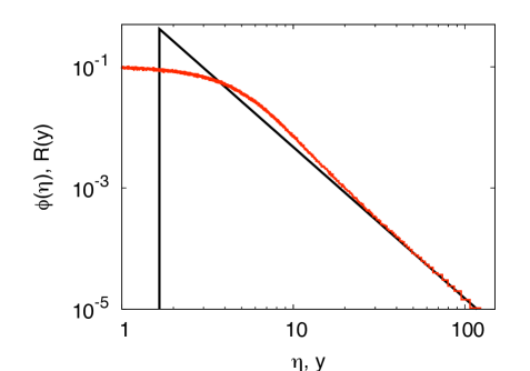
Figure 2: Case α=1.5𝛼1.5\alpha=1.5. Behavior of the right tail for ϕ(η)italic-ϕ𝜂\phi(\eta) (Black) and the the rescaled final position, y𝑦y, of free random walks of n=1000𝑛1000n=1000 step (Red). Histograms are performed using 107superscript10710^{7} samples.

We consider the case where the increments distribution ϕ(η)italic-ϕ𝜂\phi(\eta) is the symmetric Pareto distribution:

ϕ(η)={α|η|α+1,for|η|>21α0,otherwise.italic-ϕ𝜂casesotherwise𝛼superscript𝜂𝛼1for𝜂superscript21𝛼otherwise0otherwise\displaystyle\phi(\eta)=\begin{cases}&\frac{\alpha}{|\eta|^{\alpha+1}}\;,{\rm for}\;|\eta|>2^{\frac{1}{\alpha}}\\ &0\;,{\rm otherwise}.\end{cases} (56)

This distribution can be sampled efficiently using random number drawn from a uniform distribution:

η={[ran(0,12)]1α,withprobability12[ran(0,12)]1α,withprobability12;𝜂casesotherwisesuperscriptdelimited-[]ran0121𝛼withprobability12otherwisesuperscriptdelimited-[]ran0121𝛼withprobability12\displaystyle\eta=\begin{cases}&\left[\rm{ran}(0,\frac{1}{2})\right]^{-\frac{1}{\alpha}}\;,{\rm with}\,{\rm probability}\;\frac{1}{2}\\ &-\left[\rm{ran}(0,\frac{1}{2})\right]^{-\frac{1}{\alpha}}\;,{\rm with}\,{\rm probability}\;\frac{1}{2};\end{cases} (57)

where ran(0,12)ran012\rm{ran}(0,\frac{1}{2}) is a random number in the interval (0,12)012(0,\frac{1}{2}). We construct a large number of random walks, for each random walk we record the final position x(n)𝑥𝑛x(n) after n𝑛n steps and compute the correspondent rescaled variable y=xn/n1/α𝑦subscript𝑥𝑛superscript𝑛1𝛼y=x_{n}/n^{1/\alpha}. We first present our data for α=1.5𝛼1.5\alpha=1.5, for which ϕ(η)=1.5/|η|5/2italic-ϕ𝜂1.5superscript𝜂52\phi(\eta)=1.5/|\eta|^{5/2} for |η|>22/3𝜂superscript223|\eta|>2^{2/3}. For large n𝑛n the distribution of y𝑦y should converge to the a stable distribution centered around 00 and with an asymptotic tail

R(y)=32y5/2+24y4+o(y4).𝑅𝑦32superscript𝑦5224superscript𝑦4𝑜superscript𝑦4\displaystyle R(y)=\frac{3}{2\,y^{5/2}}+\frac{24}{y^{4}}+o(y^{-4})\;. (58)

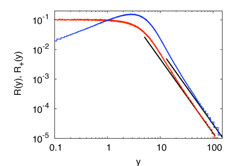
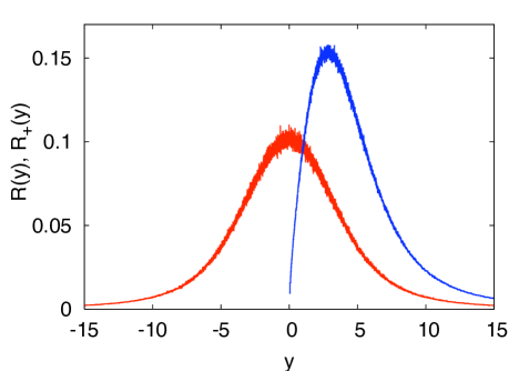
This prediction is confirmed by our direct simulation, in Fig. 2 we show that the tail of ϕ(η)italic-ϕ𝜂\phi(\eta) and R(y)𝑅𝑦R(y) coincide when η,y𝜂𝑦\eta,y\to\infty. The symmetric distribution R(y)𝑅𝑦R(y) is also plotted in Fig. 3 where we also show R+(y)subscript𝑅𝑦R_{+}(y), the histogram of the rescaled final position of the random walks constrained to be positive. R+(y)subscript𝑅𝑦R_{+}(y) is clearly defined only for positive y𝑦y, vanishes at y=0𝑦0y=0 and, when y𝑦y\to\infty, decays as c+/y5/2subscript𝑐superscript𝑦52c_{+}/y^{5/2}. One of our main prediction is that, for large y𝑦y, R+(y)/R(y)=2subscript𝑅𝑦𝑅𝑦2R_{+}(y)/R(y)=2 which means c+=3subscript𝑐3c_{+}=3 for our model. This is verified in Fig.4.
Refer to caption
Figure 3: Case α=1.5𝛼1.5\alpha=1.5. Free random walks of n=1000𝑛1000n=1000 steps (Red) and random walks constrained to be positive (Blue). Histogram are performed using 108superscript10810^{8} samples.
Refer to caption
Figure 4: Case α=1.5𝛼1.5\alpha=1.5. Free random walks of n=1000𝑛1000n=1000 steps (Red) and random walks constrained to be positive (Blue). Study of the tails. Histogram are performed using 108superscript10810^{8} samples. The expected tails: 1.5/y5/21.5superscript𝑦521.5/y^{5/2} and 3/y5/23superscript𝑦523/y^{5/2} are also drawn (Solid Line).
Refer to caption
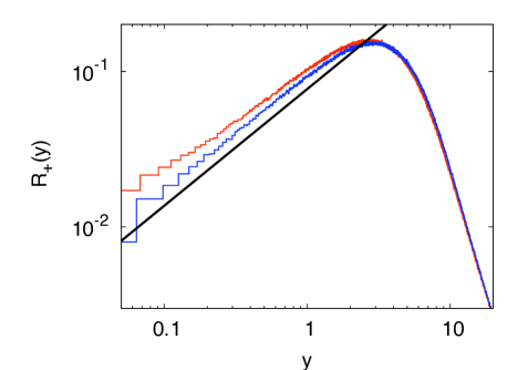
Figure 5: Case α=1.5𝛼1.5\alpha=1.5. Finite size effects for random walks constrained to be positive. Long random walks (n=5000𝑛5000n=5000 -Blue) vs short ranomd walks (n=250𝑛250n=250 - Red). Histograms are perfomed over 107superscript10710^{7} samples. The slope yα2superscript𝑦𝛼2y^{\frac{\alpha}{2}} is plotted as a guide of the eye (Black line).

III.1 Finite size effect and different values of α𝛼\alpha

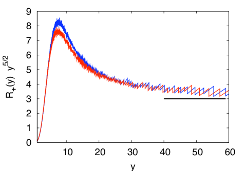
Stable distributions and universal behavior are expected in the limit of a large number of steps (i.e. n𝑛n\to\infty). In our numerical simulation the asymptotic behavior of R(y)𝑅𝑦R(y) and R+(y)subscript𝑅𝑦R_{+}(y) is studied for n=1000𝑛1000n=1000. Is this number enough to capture universality? In Fig. 5 and Fig. 6 we study how the finite number of steps affect the function R+(y)subscript𝑅𝑦R_{+}(y). Finite size effects are visible close to the boundary y=0𝑦0y=0 where, only for very large size, the distribution vanishes with the predicted exponent α/2=0.75𝛼20.75\alpha/2=0.75. For y10similar-to-or-equals𝑦10y\simeq 10 the convergence with the size n𝑛n becomes faster and the constant

c+=limyR+(y)yα+1subscript𝑐subscript𝑦subscript𝑅𝑦superscript𝑦𝛼1c_{+}=\lim_{y\to\infty}R_{+}(y)\,y^{\alpha+1} (59)

can be correctly estimated even with a moderate number of steps (see Fig.6).
Refer to caption
Figure 6: Case α=1.5𝛼1.5\alpha=1.5. Finite size effects for random walks constrained to be positive. Long random walks (n=5000𝑛5000n=5000 -Blue) vs short ranomd walks (n=250𝑛250n=250 - Red). The constant c+=3subscript𝑐3c_{+}=3 is recovered.

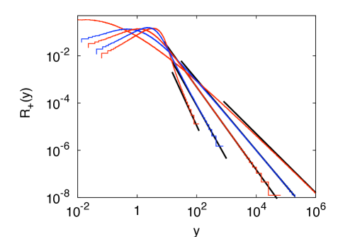
Finally we have checked that our result for c+subscript𝑐c_{+} apply to all range of 0<α<20𝛼20<\alpha<2 for symmetric Lévy flights. The asymptotic tail is more and more pronounced as α2much-less-than𝛼2\alpha\ll 2. This means that the insights given by our perturbative calculation are actually valid for all Lévy flights (see Fig.7).
Refer to caption
Figure 7: Random walks constrained to be positive for n=1000𝑛1000n=1000 steps and α=1.75,1.25,0.75,0.5,0.25𝛼1.751.250.750.50.25\alpha=1.75,1.25,0.75,0.5,0.25 (from left to right). Histograms are perfomed over 107superscript10710^{7} samples. The asymptotic behavior c+/yα+1subscript𝑐superscript𝑦𝛼1c_{+}/y^{\alpha+1} is also plotted (Black line).

III.2 Subleading corrections

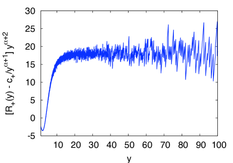
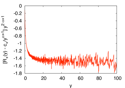
We also check the behavior of the sub-leading correction (55). For α>1𝛼1\alpha>1 this correction is expected to behave like d+yα1subscript𝑑superscript𝑦𝛼1d_{+}y^{-\alpha-1}, while for α<1𝛼1\alpha<1 we expect that it decays as d+y2α1similar-toabsentsubscript𝑑superscript𝑦2𝛼1\sim d_{+}y^{-2\alpha-1}. This prediction is confirmed in Fig. 8 for α>1𝛼1\alpha>1 and Fig. 9 for α<1𝛼1\alpha<1.

Refer to caption
Figure 8: Sub-leading correction for α=1.25>1𝛼1.251\alpha=1.25>1. Random walks constrained to be positive for n=1000𝑛1000n=1000 steps. Histograms are performed over 108superscript10810^{8} samples. The plateau reached at large y𝑦y gives a numerical estimation of d+subscript𝑑d_{+}.
Refer to caption
Figure 9: Sub-leading correction for α=0.5<1𝛼0.51\alpha=0.5<1. Random walks constrained to be positive for n=1000𝑛1000n=1000 steps. Histograms are performed over 107superscript10710^{7} samples. The plateau reached at large y𝑦y gives a numerical estimation of d+subscript𝑑d_{+}.

IV Conclusion

To conclude, we have presented a perturbative approach to the study of a Lévy flight, of index 0<α<20𝛼20<\alpha<2 on a half-line, where the perturbative parameter is ϵ=2αitalic-ϵ2𝛼\epsilon=2-\alpha. This approach, following the work of Zoia, Rosso and Kardar ZRK07 , amounts to construct a perturbative solution of the fractional Fokker-Planck equation (9) with appropriate (non-local) boundary conditions. Here, at variance with Ref. ZRK07 the perturbation theory is carried out directly for a process which is continuous both in space and time.

We have then used this perturbative method to compute, to order 𝒪(ϵ)𝒪italic-ϵ{\cal O}(\epsilon), the probability density function, R+subscript𝑅R_{+}, of the position of such a walker with an absorbing wall at the origin. A different perturbation scheme (based on path integral) was used recently WMR11 to compute the same quantity for the fractional Brownian motion, a non-Markovian process displaying anomalous diffusion. Our main result here is to give a precise conjecture, valid for any value of α𝛼\alpha, on the relation between the tail of this distribution and the tail of the steps of the random walk. Numerical simulation confirm our conjecture.

This perturbative scheme opens the way to an analytical study and can be used for any confined domain for which the Brownian solution, corresponding to α=2𝛼2\alpha=2, is known. More realistic confined geometry, like the one relevant to the scattering of solar photons, can be studied along these lines. Here we have proposed the simplest of these geometries. A first extension of the present study concerns the study of the extreme statistics of a Lévy bridge, which is a Lévy random walk on the time interval [0,t]0𝑡[0,t] constrained to start and end at the origin. Such a constrained Lévy random walk, for which little is known, has recently received some attention in statistical physics schehr_levyarea – in relation with some real-space condensation phenomena –, as well as in finance levybridge_finance . Another interesting application of such a perturbative calculation could be the study of non-intersecting Lévy walkers, the so-called ”vicious” Lévy walkers, which were recently introduced in Ref. vicious_levy .

Acknowledgements.
This work was supported by the France-Argentina MINCYT-ECOS A08E03. R. G.-G. acknowledges the hospitality at LPT and LPTMS in Orsay, A. R. and G. S acknowledge the hospitality at the Centro Atomico in Bariloche where part of this work was done. A. R. acknowledges support by ANR grant 09-BLAN-0097-02. G. S. acknowledges support by ANR grant 2011-BS04-013-01 WALKMAT.

Appendix A Perturbative scheme to order 𝒪(ϵ)𝒪italic-ϵ{\cal O}(\epsilon)

In this appendix we give a short derivation of the expression for the first correction P(1)(x,x0,t)superscript𝑃1𝑥subscript𝑥0𝑡P^{(1)}(x,x_{0},t) (II) given in Eq. (21). The equation for P(1)(x,x0,t)superscript𝑃1𝑥subscript𝑥0𝑡P^{(1)}(x,x_{0},t) reads, see Eqs. (15, II):

tP(1)(x,x0,t)=0P(1)(x,x0,t)+1P(0)(x,x0,t),subscript𝑡superscript𝑃1𝑥subscript𝑥0𝑡subscript0superscript𝑃1𝑥subscript𝑥0𝑡subscript1superscript𝑃0𝑥subscript𝑥0𝑡\partial_{t}P^{(1)}(x,x_{0},t)={\cal H}_{0}P^{(1)}(x,x_{0},t)+{\cal H}_{1}P^{(0)}(x,x_{0},t)\;, (60)

with the initial conditions P(1)(x,x0,t=0)=0superscript𝑃1𝑥subscript𝑥0𝑡00P^{(1)}(x,x_{0},t=0)=0 and P(0)(x,x0,t)superscript𝑃0𝑥subscript𝑥0𝑡P^{(0)}(x,x_{0},t) is given in (17). Eq. (60) is inhomogeneous and we can obtain its solution using the method of variation of constants. We look for a solution under the form

P(1)(x,x0,t)=cq(1)(t)ψq(x)eE(q)t𝑑q,superscript𝑃1𝑥subscript𝑥0𝑡subscriptsuperscript𝑐1𝑞𝑡subscript𝜓𝑞𝑥superscript𝑒𝐸𝑞𝑡differential-d𝑞\displaystyle P^{(1)}(x,x_{0},t)=\int c^{(1)}_{q}(t)\psi_{q}(x)e^{E(q)t}dq\;, (61)

where ψqsubscript𝜓𝑞\psi_{q} and E(q)𝐸𝑞E(q) are the eigenvectors and eigenvalues of 0subscript0{\cal H}_{0}, while the coefficient cq(1)(t)subscriptsuperscript𝑐1𝑞𝑡c^{(1)}_{q}(t) depends explicitly on time t𝑡t. Plugging Eqs. (61) and (17) into (60) one finds

𝑑qeE(q)tψq(x)tcq(1)(t)differential-dsuperscript𝑞superscript𝑒𝐸superscript𝑞𝑡subscript𝜓superscript𝑞𝑥subscript𝑡subscriptsuperscript𝑐1superscript𝑞𝑡\displaystyle\int\,dq^{\prime}\,e^{E(q^{\prime})t}\psi_{q^{\prime}}(x)\partial_{t}c^{(1)}_{q^{\prime}}(t) (62)
=𝑑qeE(q)tψq(x0)1ψq(x).absentdifferential-dsuperscript𝑞superscript𝑒𝐸superscript𝑞𝑡superscriptsubscript𝜓superscript𝑞subscript𝑥0subscript1subscript𝜓superscript𝑞𝑥\displaystyle=\int dq^{\prime}e^{E(q^{\prime})t}\psi_{q^{\prime}}^{*}(x_{0}){\cal H}_{1}\psi_{q^{\prime}}(x)\;. (63)

We multiply the left and right hand sides of Eq. (62) by ψq(x)superscriptsubscript𝜓𝑞𝑥\psi_{q}^{*}(x) and we then integrate both sides over x𝑥x. Using the normalization relation 𝑑xψq(x)ψq(x)=δ(qq)differential-d𝑥superscriptsubscript𝜓𝑞𝑥subscript𝜓superscript𝑞𝑥𝛿𝑞superscript𝑞\int\,dx\,\psi_{q}^{*}(x)\psi_{q^{\prime}}(x)=\delta(q-q^{\prime}) we obtain

eE(q)ttcq(1)(t)=𝑑qq|1|qψq(x0)eE(q)t,superscript𝑒𝐸𝑞𝑡subscript𝑡subscriptsuperscript𝑐1𝑞𝑡differential-dsuperscript𝑞quantum-operator-product𝑞subscript1superscript𝑞superscriptsubscript𝜓superscript𝑞subscript𝑥0superscript𝑒𝐸superscript𝑞𝑡\displaystyle e^{E(q)t}\partial_{t}c^{(1)}_{q}(t)=\int dq^{\prime}\langle q|{\cal H}_{1}|q^{\prime}\rangle\psi_{q^{\prime}}^{*}(x_{0})e^{E(q^{\prime})t}\;, (64)

where we have used the bra-ket notation, borrowed from Quantum Mechanics, and such that x|q=ψq(x)inner-product𝑥𝑞subscript𝜓𝑞𝑥\langle x|q\rangle=\psi_{q}(x). This can be straightforwardly integrated, using the boundary condition at time t=0𝑡0t=0

cq(1)(t)=𝑑qq|1|qψq(x0)eE(q)teE(q)tE(q)E(q).subscriptsuperscript𝑐1𝑞𝑡differential-dsuperscript𝑞quantum-operator-product𝑞subscript1superscript𝑞superscriptsubscript𝜓superscript𝑞subscript𝑥0superscript𝑒𝐸superscript𝑞𝑡superscript𝑒𝐸𝑞𝑡𝐸𝑞𝐸superscript𝑞c^{(1)}_{q}(t)=\int dq^{\prime}\langle q|{\cal H}_{1}|q^{\prime}\rangle\psi_{q^{\prime}}^{*}(x_{0})\frac{e^{E(q^{\prime})t}-e^{E(q)t}}{E(q)-E(q^{\prime})}\;. (65)

Combining (65) and (61) one obtains Eq. (II) given in the text.

Appendix B Evaluation of an integral

Here we compute the principal value of the integral entering the matrix element in Eq. (40):

I(q,q)𝐼𝑞superscript𝑞\displaystyle I(q,q^{\prime}) =\displaystyle= PV𝑑kqqk2ln|k|π2(k2q2)(k2q2)PVsuperscriptsubscriptdifferential-d𝑘𝑞superscript𝑞superscript𝑘2𝑘superscript𝜋2superscript𝑘2superscript𝑞2superscript𝑘2superscript𝑞2\displaystyle\text{PV}\int_{-\infty}^{\infty}dk\frac{qq^{\prime}k^{2}\ln|k|}{\pi^{2}(k^{2}-q^{2})(k^{2}-q^{\prime 2})} (66)
=\displaystyle= 2qqπ2PV0𝑑kk2lnk(k2q2)(k2q2).2𝑞superscript𝑞superscript𝜋2PVsuperscriptsubscript0differential-d𝑘superscript𝑘2𝑘superscript𝑘2superscript𝑞2superscript𝑘2superscript𝑞2\displaystyle\frac{2qq^{\prime}}{\pi^{2}}\text{PV}\int_{0}^{\infty}dk\frac{k^{2}\ln k}{(k^{2}-q^{2})(k^{2}-q^{\prime 2})}\;.

Without any loss of generality, since I(q,q)=I(q,q)𝐼𝑞superscript𝑞𝐼superscript𝑞𝑞I(q,q^{\prime})=I(q^{\prime},q), we assume qqsuperscript𝑞𝑞q^{\prime}\geq q. Performing the change of variable k=sq𝑘𝑠𝑞k=s\,q, one obtains straightforwardly

I(q,q)=2qπ2f1(qq)lnq+2qπ2f2(qq),𝐼𝑞superscript𝑞2superscript𝑞superscript𝜋2subscript𝑓1superscript𝑞𝑞𝑞2superscript𝑞superscript𝜋2subscript𝑓2superscript𝑞𝑞\displaystyle I(q,q^{\prime})=\frac{2q^{\prime}}{\pi^{2}}f_{1}\left(\frac{q^{\prime}}{q}\right)\ln{q}+\frac{2q^{\prime}}{\pi^{2}}f_{2}\left(\frac{q^{\prime}}{q}\right)\;, (67)

where

f1(x)=PV0𝑑ss2(s21)(s2x2),subscript𝑓1𝑥PVsuperscriptsubscript0differential-d𝑠superscript𝑠2superscript𝑠21superscript𝑠2superscript𝑥2\displaystyle f_{1}(x)=\text{PV}\int_{0}^{\infty}ds\frac{s^{2}}{(s^{2}-1)(s^{2}-x^{2})}\;, (68)
f2(x)=PV0𝑑ss2lns(s21)(s2x2).subscript𝑓2𝑥PVsuperscriptsubscript0differential-d𝑠superscript𝑠2𝑠superscript𝑠21superscript𝑠2superscript𝑥2\displaystyle f_{2}(x)=\text{PV}\int_{0}^{\infty}ds\frac{s^{2}\ln s}{(s^{2}-1)(s^{2}-x^{2})}\;. (69)

We notice that f2(x)subscript𝑓2𝑥f_{2}(x) can be written as

f2(x)=f1(x)lnx+PV0𝑑ss2ln(s/x)(s21)(s2x2).subscript𝑓2𝑥subscript𝑓1𝑥𝑥PVsuperscriptsubscript0differential-d𝑠superscript𝑠2𝑠𝑥superscript𝑠21superscript𝑠2superscript𝑥2f_{2}(x)=f_{1}(x)\ln x+\text{PV}\int_{0}^{\infty}ds\,s^{2}\frac{\ln(s/x)}{(s^{2}-1)(s^{2}-x^{2})}\;. (70)

The purpose of this trick (70) is that the integrand has now only a simple pole in s=1𝑠1s=1 so that, taking the principal value, yields a perfectly smooth function of x𝑥x. This integral can then be evaluated to yield:

f2(x)=f1(x)lnx+π24(1+x),subscript𝑓2𝑥subscript𝑓1𝑥𝑥superscript𝜋241𝑥\displaystyle f_{2}(x)=f_{1}(x)\ln x+\frac{\pi^{2}}{4(1+x)}\;, (71)

so that one has

I(q,q)=2qπ2f1(qq)lnq+qq2(q+q).𝐼𝑞superscript𝑞2superscript𝑞superscript𝜋2subscript𝑓1superscript𝑞𝑞superscript𝑞𝑞superscript𝑞2𝑞superscript𝑞\displaystyle I(q,q^{\prime})=\frac{2q^{\prime}}{\pi^{2}}f_{1}\left(\frac{q^{\prime}}{q}\right)\ln{q^{\prime}}+\frac{q\,q^{\prime}}{2(q+q^{\prime})}\;. (72)

Looking at the expression of f1(x)subscript𝑓1𝑥f_{1}(x) above (68), one sees that for x=1𝑥1x=1, the integrand has a double pole in s=1𝑠1s=1 and one thus expects f1(x)subscript𝑓1𝑥f_{1}(x) to be highly singular in x=1𝑥1x=1. To characterize it, we compute its Fourier transform

f^1(p)=20𝑑xf1(x)cos(px),subscript^𝑓1𝑝2superscriptsubscript0differential-d𝑥subscript𝑓1𝑥𝑝𝑥\displaystyle\hat{f}_{1}(p)=2\int_{0}^{\infty}dxf_{1}(x)\cos{(px)}\;, (73)

which yields after straightforward manipulations of Eq. (68) (which can be done e.g. with Mathematica)

f^1(p)=π22cosp,subscript^𝑓1𝑝superscript𝜋22𝑝\displaystyle\hat{f}_{1}(p)=\frac{\pi^{2}}{2}\cos{p}\;, (74)

which yields

f1(qq)=π2q4δ(qq),subscript𝑓1superscript𝑞𝑞superscript𝜋2𝑞4𝛿𝑞superscript𝑞\displaystyle f_{1}\left(\frac{q^{\prime}}{q}\right)=\frac{\pi^{2}q}{4}\delta(q-q^{\prime})\;, (75)

and finally

I(q,q)=δ(qq)12q2lnq+qq2(q+q),𝐼𝑞superscript𝑞𝛿𝑞superscript𝑞12superscript𝑞2𝑞𝑞superscript𝑞2𝑞superscript𝑞\displaystyle I(q,q^{\prime})=\delta(q-q^{\prime})\frac{1}{2}q^{2}\ln q+\frac{q\,q^{\prime}}{2(q+q^{\prime})}\;, (76)

which is used in the Eq. (40) in the text.

Appendix C Details about the perturbative calculation of the propagator with an absorbing wall

This appendix is devoted to the analysis of Z(1)(y,y0)superscript𝑍1𝑦subscript𝑦0Z^{(1)}(y,y_{0}) given by the sum of the two terms in Eqs. (41, 42, 43) in the limit y00subscript𝑦00y_{0}\to 0. The first term ZA(y,y0)subscript𝑍𝐴𝑦subscript𝑦0Z_{A}(y,y_{0}) is easy to analyse and yields

ZA(y,y0)=2y0yR(1)(y)+𝒪(y02),subscript𝑍𝐴𝑦subscript𝑦02subscript𝑦0subscript𝑦superscript𝑅1𝑦𝒪superscriptsubscript𝑦02\displaystyle Z_{A}(y,y_{0})=-2y_{0}\partial_{y}R^{(1)}(y)+{\cal O}(y_{0}^{2})\;, (77)

where R(1)(y)superscript𝑅1𝑦R^{(1)}(y) admits the integral representation given in Eq. (32).

The analysis of the small y0subscript𝑦0y_{0} behavior of ZB(y,y0)subscript𝑍𝐵𝑦subscript𝑦0Z_{B}(y,y_{0}) given in Eq. (43) is more subtle. To deal with this double integral over k1subscript𝑘1k_{1} and k2subscript𝑘2k_{2}, we first make the change of variable k1=usubscript𝑘1superscript𝑢k_{1}=u^{\prime} and k2=uusubscript𝑘2𝑢superscript𝑢k_{2}=uu^{\prime} and observe that the integral over usuperscript𝑢u^{\prime} can then be performed to yield

ZB(y,y0)=14π0duu(u1)(u+1)2[e(y+uy0)24\displaystyle Z_{B}(y,y_{0})=\frac{1}{4\sqrt{\pi}}\int_{0}^{\infty}du\frac{u}{(u-1)(u+1)^{2}}\Bigg{[}e^{-\frac{(y+uy_{0})^{2}}{4}}
e(yuy0)24+1u(e(yuy0)24u2e(y+uy0)24u2)].\displaystyle-e^{-\frac{(y-uy_{0})^{2}}{4}}+\frac{1}{u}\left(e^{-\frac{(y-uy_{0})^{2}}{4u^{2}}}-e^{-\frac{(y+uy_{0})^{2}}{4u^{2}}}\right)\Bigg{]}\;. (78)

Using now the identity

u(u1)(u+1)2=1(u+1)2+1(u1)(u+1)2,𝑢𝑢1superscript𝑢121superscript𝑢121𝑢1superscript𝑢12\displaystyle\frac{u}{(u-1)(u+1)^{2}}=\frac{1}{(u+1)^{2}}+\frac{1}{(u-1)(u+1)^{2}}\;, (79)

we split ZB(y,y0)subscript𝑍𝐵𝑦subscript𝑦0Z_{B}(y,y_{0}) into two parts:

ZB(y,y0)=14π(1(y,y0)+2(y,y0)),subscript𝑍𝐵𝑦subscript𝑦014𝜋subscript1𝑦subscript𝑦0subscript2𝑦subscript𝑦0\displaystyle Z_{B}(y,y_{0})=\frac{1}{4\sqrt{\pi}}({\cal I}_{1}(y,y_{0})+{\cal I}_{2}(y,y_{0}))\;, (80)

where

1(y,y0)subscript1𝑦subscript𝑦0\displaystyle{\cal I}_{1}(y,y_{0}) =\displaystyle= 0du(u+1)2[e(y+uy0)24e(yuy0)24\displaystyle\int_{0}^{\infty}\frac{du}{(u+1)^{2}}\Bigg{[}e^{-\frac{(y+uy_{0})^{2}}{4}}-e^{-\frac{(y-uy_{0})^{2}}{4}} (81)
+\displaystyle+ 1u(e(yuy0)24u2e(y+uy0)24u2)],\displaystyle\frac{1}{u}\left(e^{-\frac{(y-uy_{0})^{2}}{4u^{2}}}-e^{-\frac{(y+uy_{0})^{2}}{4u^{2}}}\right)\Bigg{]}\;,
2(z,w)subscript2𝑧𝑤\displaystyle{\cal I}_{2}(z,w) =\displaystyle= 0du(u1)(u+1)2[e(y+uy0)24e(yuy0)24\displaystyle\int_{0}^{\infty}\frac{du}{(u-1)(u+1)^{2}}\Bigg{[}e^{-\frac{(y+uy_{0})^{2}}{4}}-e^{-\frac{(y-uy_{0})^{2}}{4}} (82)
+\displaystyle+ 1u(e(yuy0)24u2e(u+uy0)24u2)].\displaystyle\frac{1}{u}\left(e^{-\frac{(y-uy_{0})^{2}}{4u^{2}}}-e^{-\frac{(u+uy_{0})^{2}}{4u^{2}}}\right)\Bigg{]}\;.

In 2(y,y0)subscript2𝑦subscript𝑦0{\cal I}_{2}(y,y_{0}) (82) the small y0subscript𝑦0y_{0} limit can be taken easily. It yields

2(y,y0)subscript2𝑦subscript𝑦0\displaystyle{\cal I}_{2}(y,y_{0}) =\displaystyle= yy00du(u1)(u+1)2(1u2ey24u2uey24)𝑦subscript𝑦0superscriptsubscript0𝑑𝑢𝑢1superscript𝑢121superscript𝑢2superscript𝑒superscript𝑦24superscript𝑢2𝑢superscript𝑒superscript𝑦24\displaystyle y\,y_{0}\int_{0}^{\infty}\frac{du}{(u-1)(u+1)^{2}}\left(\frac{1}{u^{2}}e^{-\frac{y^{2}}{4u^{2}}}-ue^{-\frac{y^{2}}{4}}\right) (83)
+\displaystyle+ 𝒪(y02).𝒪superscriptsubscript𝑦02\displaystyle{\cal O}(y_{0}^{2})\;.

We now decompose 1(y,y0)subscript1𝑦subscript𝑦0{\cal I}_{1}(y,y_{0}) (82) into two parts

1(y,y0)=11(y,y0)+12(y,y0),subscript1𝑦subscript𝑦0subscript11𝑦subscript𝑦0subscript12𝑦subscript𝑦0\displaystyle{\cal I}_{1}(y,y_{0})={\cal I}_{11}(y,y_{0})+{\cal I}_{12}(y,y_{0})\;, (84)
11(y,y0)=0du(u+1)2(e(y+uy0)24e(yuy0)24),subscript11𝑦subscript𝑦0superscriptsubscript0𝑑𝑢superscript𝑢12superscript𝑒superscript𝑦𝑢subscript𝑦024superscript𝑒superscript𝑦𝑢subscript𝑦024\displaystyle{\cal I}_{11}(y,y_{0})=\int_{0}^{\infty}\frac{du}{(u+1)^{2}}\left(e^{-\frac{(y+uy_{0})^{2}}{4}}-e^{-\frac{(y-uy_{0})^{2}}{4}}\right)\;,
12(y,y0)=0duu(u+1)2(e(yuy0)24u2e(y+uy0)24u2).subscript12𝑦subscript𝑦0superscriptsubscript0𝑑𝑢𝑢superscript𝑢12superscript𝑒superscript𝑦𝑢subscript𝑦024superscript𝑢2superscript𝑒superscript𝑦𝑢subscript𝑦024superscript𝑢2\displaystyle{\cal I}_{12}(y,y_{0})=\int_{0}^{\infty}\frac{du}{u(u+1)^{2}}\left(e^{-\frac{(y-uy_{0})^{2}}{4u^{2}}}-e^{-\frac{(y+uy_{0})^{2}}{4u^{2}}}\right)\;.

In 12(y,y0)subscript12𝑦subscript𝑦0{\cal I}_{12}(y,y_{0}), it is straightforward to obtain the small y0subscript𝑦0y_{0} behavior as

12(y,y0)=yy00duu2(u+1)2ey24u2+𝒪(y02).subscript12𝑦subscript𝑦0𝑦subscript𝑦0superscriptsubscript0𝑑𝑢superscript𝑢2superscript𝑢12superscript𝑒superscript𝑦24superscript𝑢2𝒪superscriptsubscript𝑦02{\cal I}_{12}(y,y_{0})=y\,y_{0}\int_{0}^{\infty}\frac{du}{u^{2}(u+1)^{2}}e^{-\frac{y^{2}}{4u^{2}}}+{\cal O}(y_{0}^{2})\;. (85)

The integral in 11(y,y0)subscript11𝑦subscript𝑦0{\cal I}_{11}(y,y_{0}) contains a logarithmic singularity when y00subscript𝑦00y_{0}\to 0, which is a bit tricky to extract. To do so, we first perform a change of variable s=y0u𝑠subscript𝑦0𝑢s=y_{0}\,u and then add and substract the term y00𝑑s(ey2/4ey2/4ys)/(s+y0)2subscript𝑦0superscriptsubscript0differential-d𝑠superscript𝑒superscript𝑦24superscript𝑒superscript𝑦24𝑦𝑠superscript𝑠subscript𝑦02y_{0}\int_{0}^{\infty}ds(e^{-y^{2}/4}-e^{-y^{2}/4-ys})/(s+y_{0})^{2}. Now using

0𝑑s1(s+y0)2(eys1)superscriptsubscript0differential-d𝑠1superscript𝑠subscript𝑦02superscript𝑒𝑦𝑠1\displaystyle\int_{0}^{\infty}ds\frac{1}{(s+y_{0})^{2}}\left(e^{-ys}-1\right) =\displaystyle= y(logy0+logy+γE)𝑦subscript𝑦0𝑦subscript𝛾𝐸\displaystyle y(\log{y_{0}}+\log{y}+\gamma_{E}) (86)
+\displaystyle+ 𝒪(y0logy0),𝒪subscript𝑦0subscript𝑦0\displaystyle{\cal O}(y_{0}\log y_{0})\;,

one obtains, for y00subscript𝑦00y_{0}\to 0:

11(y,y0)subscript11𝑦subscript𝑦0\displaystyle{\cal I}_{11}(y,y_{0}) =\displaystyle= (y0logy0)yey24+y0yey2/4(γE+logy)subscript𝑦0subscript𝑦0𝑦superscript𝑒superscript𝑦24subscript𝑦0𝑦superscript𝑒superscript𝑦24subscript𝛾𝐸𝑦\displaystyle(y_{0}\log{y_{0}})\,ye^{-\frac{y^{2}}{4}}+y_{0}ye^{-y^{2}/4}\left(\gamma_{E}+\log{y}\right) (87)
\displaystyle- y0ey2/4𝒬(y)+𝒪(y02logy0),subscript𝑦0superscript𝑒superscript𝑦24𝒬𝑦𝒪superscriptsubscript𝑦02subscript𝑦0\displaystyle y_{0}e^{-y^{2}/4}{\cal Q}(y)+{\cal O}(y_{0}^{2}\log y_{0})\;,

where

𝒬(y)=0dss2(eys1+2es24sinh(ys2)),𝒬𝑦superscriptsubscript0𝑑𝑠superscript𝑠2superscript𝑒𝑦𝑠12superscript𝑒superscript𝑠24𝑦𝑠2{\cal Q}(y)=\int_{0}^{\infty}\frac{ds}{s^{2}}\left(e^{-ys}-1+2\,e^{-\frac{s^{2}}{4}}\sinh{\left(\frac{y\,s}{2}\right)}\right)\;, (88)

Finally combining Eqs. (83), (85) and (87) one obtains the small y0subscript𝑦0y_{0} behavior of ZB(y,y0)subscript𝑍𝐵𝑦subscript𝑦0Z_{B}(y,y_{0}) in Eq. (80) as

ZB(y,y0)=yey244π[(y0lny0)\displaystyle Z_{B}(y,y_{0})=\frac{ye^{-\frac{y^{2}}{4}}}{4\sqrt{\pi}}\Bigg{[}(y_{0}\ln{y_{0}})
\displaystyle- y0(𝒬(y)yγEln(y)𝒜(y))]+𝒪(y02lny0),\displaystyle y_{0}\left(\frac{{\cal Q}(y)}{y}-\gamma_{E}-\ln{(y)}-{\cal A}(y)\right)\Bigg{]}+{\cal O}(y_{0}^{2}\ln y_{0})\;,

where 𝒜(y)𝒜𝑦{\cal A}(y) is given by

𝒜(y)=0𝑑u1(u1)(u+1)2[1uey24(1u21)u].𝒜𝑦superscriptsubscript0differential-d𝑢1𝑢1superscript𝑢12delimited-[]1𝑢superscript𝑒superscript𝑦241superscript𝑢21𝑢{\cal A}(y)=\int_{0}^{\infty}du\frac{1}{(u-1)(u+1)^{2}}\left[\frac{1}{u}e^{-\frac{y^{2}}{4}\left(\frac{1}{u^{2}}-1\right)}-u\right]\;. (90)

One can then obtain Z(y,y0)=Z(0)(y,y0)ϵ(ZA(y,y0)+ZB(y,y0))𝑍𝑦subscript𝑦0superscript𝑍0𝑦subscript𝑦0italic-ϵsubscript𝑍𝐴𝑦subscript𝑦0subscript𝑍𝐵𝑦subscript𝑦0Z(y,y_{0})=Z^{(0)}(y,y_{0})-\epsilon(Z_{A}(y,y_{0})+Z_{B}(y,y_{0})) in the limit y00subscript𝑦00y_{0}\to 0 from the Eqs. (45), (77) and (C) as:

Z(y,y0)=y0(1ϵ2lny0)y2πey24ϵy0Z~1(y),𝑍𝑦subscript𝑦0subscript𝑦01italic-ϵ2subscript𝑦0𝑦2𝜋superscript𝑒superscript𝑦24italic-ϵsubscript𝑦0subscript~𝑍1𝑦Z(y,y_{0})=y_{0}(1-\frac{\epsilon}{2}\ln{y_{0}})\frac{y}{2\sqrt{\pi}}e^{-\frac{y^{2}}{4}}-\epsilon y_{0}\tilde{Z}_{1}(y)\;, (91)

where Z~1(z)subscript~𝑍1𝑧\tilde{Z}_{1}(z) can be read off straightfowardly from Eqs. (77) and (C):

Z~1(y)=2yR(1)(y)subscript~𝑍1𝑦2subscript𝑦superscript𝑅1𝑦\displaystyle\tilde{Z}_{1}(y)=-2\partial_{y}R^{(1)}(y) (92)
y4πey2/4(𝒬(y)yγElny𝒜(y)).𝑦4𝜋superscript𝑒superscript𝑦24𝒬𝑦𝑦subscript𝛾𝐸𝑦𝒜𝑦\displaystyle-\frac{\,y}{4\sqrt{\pi}}e^{-y^{2}/4}\left(\frac{{\cal Q}(y)}{y}-\gamma_{E}-\ln{y}-{\cal A}(y)\right)\;.

This perturbative expansion (91) is fully consistent with the expected behavior ZK95 ; zoia_semi_inf

Z(y,y0)y0α2Z~(y),y00,Z~(y)=Z~(0)(y)ϵZ~(1)(y),formulae-sequencesimilar-to𝑍𝑦subscript𝑦0superscriptsubscript𝑦0𝛼2~𝑍𝑦formulae-sequencesubscript𝑦00~𝑍𝑦superscript~𝑍0𝑦italic-ϵsuperscript~𝑍1𝑦Z(y,y_{0})\sim y_{0}^{\frac{\alpha}{2}}\tilde{Z}(y)\;,\;y_{0}\to 0\;,\tilde{Z}(y)=\tilde{Z}^{(0)}(y)-\epsilon\tilde{Z}^{(1)}(y)\;, (93)

where Z~(1)(y)superscript~𝑍1𝑦\tilde{Z}^{(1)}(y) is given in Eq. (92). These integrals that enter the definition of Z~(1)(y)superscript~𝑍1𝑦\tilde{Z}^{(1)}(y) can then be computed, for instance using Mathematica, to yield the following expression of R+(y)subscript𝑅𝑦R_{+}(y) from Eq. (44):

R+(y)=R+(0)(y)(1+ϵW+(y)+𝒪(ϵ2)),subscript𝑅𝑦superscriptsubscript𝑅0𝑦1italic-ϵsubscript𝑊𝑦𝒪superscriptitalic-ϵ2\displaystyle R_{+}(y)=R_{+}^{(0)}(y)\left(1+\epsilon W_{+}(y)+{\cal O}(\epsilon^{2})\right)\;, (94)
W+(y)=148[6024γE48log2y2(186γE12log2)6(2πy)ey24\displaystyle W_{+}(y)=\frac{1}{48}\Bigg{[}60-24\gamma_{E}-48\log{2}-y^{2}(18-6\gamma_{E}-12\log{2})-6(2-\sqrt{\pi}y)e^{\frac{y^{2}}{4}}
+y2(y24)y422F2(1,1;52,3;y24)24πyey24Erf(y2)3π(y22)Erfi(y2)+3(y24)Ei(y24)],\displaystyle+y^{2}(y^{2}-4)\frac{y^{4}}{2}\,_{2}F_{2}\left({1,1};{\frac{5}{2},3};\frac{y^{2}}{4}\right)-\frac{24\sqrt{\pi}}{y}e^{\frac{y^{2}}{4}}{\rm Erf}\left(\frac{y}{2}\right)-3\pi(y^{2}-2){\rm Erfi}\left(\frac{y}{2}\right)+3(y^{2}-4){\rm Ei}\left(\frac{y^{2}}{4}\right)\Bigg{]}\;,

where R+(0)(y)superscriptsubscript𝑅0𝑦R_{+}^{(0)}(y) is given in Eq. (46) and F22(1,1;52,3;u)subscriptsubscript𝐹2211523𝑢\,{}_{2}F_{2}\left({1,1};{\frac{5}{2},3};u\right) is a hypergeometric series abramowitz . From this expression (94) it is straightforward to obtain the asymptotic behaviors given in the text (48, 49).

References

  • (1) E. Sparre-Andersen, Math. Scand. 1, 263 (1953); Math. Scand. 2, 195 (1954).
  • (2) W. Feller, An introduction to Probability Theory and its Applications (Wiley), New York (1968).
  • (3) B. D. Hughes, Random Walks and Random Environments, Vol. 1, Clarendon Press, Oxford, (1996).
  • (4) E. W. Montroll, G. H. Weiss, J. Math. Phys. 6, 167 (1965).
  • (5) J.-P. Bouchaud, A. Georges, Phys. Rep. 195, 127 (1990).
  • (6) R. Metzler, J. Klafter, Phys. Rep. 339, 1 (2000).
  • (7) S. N. Majumdar, Physica A 389 (20), 4299 (2010), arXiv:0912.2586.
  • (8) V. Pareto, Cours d’économie politique. Reprinted as a volume of Oeuvres complètes. (Droz, Geneva, 1896-1965).
  • (9) B. B. Mandelbrot, Journal of Business, 36 394 (1963).
  • (10) M. F. Shlesinger, G. M. Zaslavsky, U. Frisch Eds., Lévy Flights and Related Topics in Physics (Proc. Nice, France; Springer Verlag, 1994).
  • (11) G. Biroli, J.-P. Bouchaud, M. Potters, Europhys. Lett. 78, 10001 (2007).
  • (12) N. Mercadier, W. Guérin, M. Chevallier, R. Kaiser, Nature Physics 5, 602 (2009).
  • (13) A. Davis, A. Marshak, in M. M. Novak, T. G. Dewey (Eds.), Fractal frontiers, World Science, River Edge, N J, p. 63 (1997).
  • (14) K. Pfeilsticker, J. Geophys. Res. D 104, 4101 (1999).
  • (15) A. Davis, K. Pfeilsticker, A. Marshak, in Proceedings of 10th AMS Conference on Atmospheric Radiation, pp. 575-578, American Meteorological Society, Boston, Massachusetts.
  • (16) E. P. Raposo, S. V. Buldyrev, M. G. E. da Luz, G. M. Vishwanathan, J. Phys. A: Math. Theor. 42, 434003 (2009).
  • (17) M. Yor, Exponential functionals of Brownian motion and related processes (Springer), Berlin (2001).
  • (18) S. N. Majumdar, Current Science 89, 2076 (2005).
  • (19) I. Podlubny, Fractional Differential Equations (Academic Press, London, 1999).
  • (20) S. G. Samko, A. A. Kilbas and O. I. Maritchev, Fractional Integrals and Derivatives (Gordon and Breach, New York, 1993).
  • (21) G. Zumofen, J. Klafter, Phys. Rev. E 51, 2805 (1995).
  • (22) A. V. Chechkin, R. Metzler, V. Y. Gonchar, J. Klafter, L. V. Tanatarov, J. Phys. A.: Math. Gen. 36, L537 (2003).
  • (23) A. Zoia, A. Rosso, M. Kardar, Phys. Rev. E 76, 021116 (2007).
  • (24) V. V. Ivanov, Astron. Astroph. 286, 328 (1994).
  • (25) A. Zoia, A. Rosso, S. N. Majumdar, Phys. Rev. Lett. 102, 120602 (2009).
  • (26) D. A. Darling, Trans. Am. Math. Soc., 83, 164 (1956).
  • (27) V. B. Nevzorov, J. Soviet Math. 20, 2221 (1982).
  • (28) K. J. Wiese, S. N. Majumdar, A. Rosso, Phys. Rev. E 83, 061141 (2011).
  • (29) G. Schehr, S. N. Majumdar, J. Stat. Mech. P08005 (2010).
  • (30) E. Hoylea, L. P. Hughstona, A. Macrina, Stoch. Proc. Appl. 121(4), 856 (2011), arXiv:0912.3652.
  • (31) I. Goncharenko, A. Gopinathan, Phys. Rev. Lett. 105, 190601 (2010).
  • (32) M. Abramowitz, I. A. Stegun in Handbook of Mathematical Functions (Dover, New York, 1973).