Radio observations of the first three-month $\it{Fermi}$-AGN at 4.8 GHz

Abstract

Using the Urumqi 25 m radio telescope, sources from the first three-month $\it{Fermi}$-LAT detected AGN catalog with declination $>0^{\circ}$ were observed in 2009 at 4.8 GHz. The radio flux density appears to correlate with the $\gamma$-ray intensity. Intra-day variability (IDV) observations were performed in March, April and May in 2009 for selected 42 $\gamma$-ray bright blazars, and $\sim$60% of them show evident flux variability at 4.8 GHz during the IDV observations, the IDV detection rate is higher than that in previous flat-spectrum AGN samples. The IDV appears more often in the VLBI-core dominant blazars, and the non-IDV blazars show relatively ‘steeper’ spectral indices than the IDV blazars. Pronounced inter-month variability has been found in two BL Lac objects: J0112+2244 and J0238+1636.

1 Introduction

In the 1990s the space $\gamma$-ray telescope EGRET (the Energetic Gamma Ray Experiment Telescope) identified 66 blazars during its mission (Hartman et al. 1999). $\it{Fermi}$ (the Fermi Gamma Ray Space Telescope spacecraft), the successor of EGRET, launched in 2008, is now in all-sky survey mission. $\it{Fermi}$ has a much higher sensitivity and pointing accuracy than EGRET, and has already detected more AGN (Active Galactic Nuclei), see Abdo et al. (2010). The first three-month observations of the $\it{Fermi}$-LAT (Large Area Telescope on board the Fermi Gamma Ray Space Telescope spacecraft) detected 132 bright $\gamma$-ray sources in which 104 are blazars (Abdo et al. 2009). Some of the $\it{Fermi}$-LAT detected AGN exhibit $\gamma$-ray variability on timescales of days.

Blazars are either flat-spectrum radio quasars or BL Lac objects, and they are extremely variable at all observable wavelengths on timescales ranging from less than an hour to many years, both in total power and linear polarization. The apparent motions of VLBI (Very long Baseline Interferometry) components along their jets are often highly superluminal with brightness temperatures being close to the inverse-Compton limit. Such violent behaviour in blazars is attributed to relativistic jets oriented very close to the line of sight (Rees 1966; Urry & Padovani 1995). The relationship of variability at different wavelengths is a crucial test for theoretical models of these outbursts/flares in $\gamma$-ray AGN.

Although it is generally accepted that the $\gamma$-rays detected from blazars are emitted from collimated jets of charged particles moving at relativistic speeds (Maraschi et al. 1992), open questions remain. The mechanisms by which the particles are accelerated, the precise site of the $\gamma$-ray production, the origin of AGN variability and the $\gamma$-ray duty cycle of blazars are still not well understood.

IDV (Intra-Day Variability, rapid variability on timescales of few hours to few days) observation and radio monitoring can provide the variability characteristics of AGN in radio, allowing us to search for correlations between radio and $\gamma$-ray luminosities and to study the connection between the emission mechanisms.

Intraday variability of radio flux density has been found in about 30% to 50% of the flat-spectrum radio sources (Quirrenbach et al. 1992; Lovell et al. 2008). If interpreted as being source intrinsic, the rapid variability would imply micro-arcsecond scale sizes of the emitting regions, which would result in excessively large apparent brightness temperatures far in excess of the inverse-Compton limit of $\sim\rm 10^{12}K$ (Kellermann & Pauliny-Toth 1969; Readhead 1994). Thus, theories which explain IDV with variations intrinsic to the blazars, require either excessively large Doppler boosting factors or special source geometries (such as non-spherical relativistic emission models, e.g. Qian et al. 1996) or coherent and collective plasma emission (Benford 1992; Lesch & Pohl 1992) to avoid the inverse-Compton catastrophe. Alternatively, IDV was explained by interstellar scintillation (ISS), especially for very rapid variables such as PKS 0405$-$385, J1819+384, PKS 1257$-$326 and J1128+592 (Kedziora-Chudczer et al. 1997; Dennett-Thorpe & de Bruyn 2000; Bignall et al. 2003; Gabanyi et al. 2009 respectively).

Almost all the $\it{Fermi}$-LAT detected AGN are blazars. There appears a significant correlation between the radio flux density at 15 GHz and $\gamma$-ray flux density of the $\it{Fermi}$-LAT AGN (Ackermann et al. 2011). It is expected that the $\it{Fermi}$-AGN are more IDV-active than non $\gamma$-ray AGN. Dedicated IDV and flux density monitoring observations are needed to study the variability on different timescales and to correlate the occurrence of IDV with the $\gamma$-ray activity of the $\it{Fermi}$-AGN. In March 2009, we launched a program with the 25-m Urumqi radio telescope at 4.8 GHz to investigate the intra-day to inter-month variability of the first three-month $\it{Fermi}$-detected AGN. We aim at searching for new IDV sources, and for a statistical comparison of the radio and the $\gamma$-ray emission of $\it{Fermi}$-detected AGN.

In this paper, we present the results from our single dish radio observations of the $\it{Fermi}$-LAT detected AGN with declination $>0^{\circ}$. We adopt $S\propto\nu^{\alpha}$ to define a spectral index throughout the paper.

2 The sample and observations

Our sample is selected from the first three-month $\it{Fermi}$-LAT detected AGN catalog (Abdo et al. 2009). We originally observed 63 sources with declination $>0^{\circ}$ from the catalog as our pilot ‘cross-scan’ observations in March 2009. Thirteen sources were rejected due to poor data quality in the pilot run. Flux densities of 50 sources were obtained in the pilot observation at 4.8 GHz, including the galaxy NGC1275 (3C84). We selected the sources for IDV observation from the 50 sources by following criteria:

1. Blazars with source brightness: $S_{4.8GHz}>$ 0.3 Jy.

2. Source compactness: measured full-width-half-maximum (FWHM) of source brightness profile $<$ 700''  which is $\sim$1.2 times the antenna beam size at 4.8 GHz. Extended source brightness profile may indicate a confusion between the target and its nearby sources which cannot be resolved by the 25-m radio telescope at 4.8 GHz.

The criteria restrict the number of the sources for IDV observation to be 45, unfortunately 3 of them, namely J0920+4441, J1229+0203 (3C273) and J1253+5301 were not involved in afterwards IDV campaign by mistake. Therefore, the sources which IDV observations were carried out are 42, which consists of 24 flat-spectrum radio quasars and 18 BL Lac objects.

The IDV observations were carried out in order to study the short time-scale variability of the $\gamma$-ray bright blazars. These sources were also planned to monitor monthly from March to December in 2009 at 4.8 GHz. Since all of the selected sources are strong and compact, both the IDV observations and the flux monitoring were performed in ‘cross-scan’ mode.

2.1 IDV observations

The three IDV observing sessions performed with the Urumqi telescope are summarized in Table 1; column 1 the symbols for different epochs; column 2 the starting and ending dates of the experiments; column 3 the duration; column 4 the mean number of flux density measurements per hour; column 5 the number of observed sources (including the calibrators, usually we use 3C286, 3C48 and NGC7027 as primary calibrators, B0836+710 and B0951+699 etc as secondary calibrators); column 6 the average number of measurements per hour for each $\it Fermi$ blazar (duty cycle, which represents the shortest time scale on which we can search for variability); column 7 the average modulation index of calibrators, which is probably the most important since it reflects the conditions of the observation (the lower the $m_{0}$ the better the weather, and/or the more stable the receiver) and will be described in the following sections.

Table 1: Summary of the IDV observations for the 42 selected $\it Fermi$ blazars

Epoch	Date	Duration	Average	Number of	Duty cycle for	$m_{0}$
		[$d$]	sampling [$h^{-1}$]	observed sources	$\it Fermi$ blazars [$h^{-1}$]	[%]
(1)	(2)	(3)	(4)	(5)	(6)	(7)
A	21/03/09 - 25/03/09	4.8	11.2	49	0.3	0.6
B	19/04/09 - 24/04/09	5.3	10.8	37	0.4	0.7
C	06/05/09 - 09/05/09	3.8	10.1	17	0.8	0.6

2.2 Inter-month observations

The 42-blazar sample was also planned to be monitored monthly from March to December in 2009 at 4.8 GHz. Each source was at least measured once in an individual observation. Sometimes the flux density measurements were repeated for sources whose observations were affected by adverse conditions such as bad weather and low elevation. Actually, not all sources were observed every month due to time limitation, so that some sources have no data in some months. In fact no data in June 2009 for all sources.

3 Data calibration

All observations have been done in ‘cross-scan’ mode with a central frequency of 4800 MHz and a bandwidth of 600 MHz, see Sun et al. (2007) for a description of the observing system. Each scan consists of 8 sub-scans in azimuth and elevation over the source position, fourfold in each coordinate. This enables us to check the pointing offsets in both coordinates. After applying a correction for small pointing offsets, the amplitudes of both azimuth and elevation are averaged. Then, we correct the measurements for the elevation dependent antenna gain and the remaining systematic time-dependent effects by using a number of steep spectrum and non-variable secondary calibrators. Finally, we convert our measurements to absolute flux density. The conversion factor is determined as the average scale of the frequently observed primary calibrator’s assumed flux densities (Baars et al. 1977; Ott et al. 1994) by the measured temperatures, where we use the assumed flux density of 7.53 Jy, 5.53 Jy and 5.47 Jy at 4.8 GHz for the primary calibrators 3C286, 3C48 and NGC7027 respectively in our data reduction.

The overall typical error on a single measurement is around 0.3-1.5% of source flux density depending e.g. on weather conditions and source intensity, usually weaker sources have larger errors in individual measurements. Our data reduction of the radio flux density has an essentially similar procedure to the Effelsberg data reduction (e.g. Kraus et al. 2003). Actually we have made simultaneous IDV observations with Urumqi and Effelsberg telescopes as early as April 2006, we obtained consistent results between the two telescopes.

After the data reduction described above, the light curves of the sources were obtained. In Fig. 1 we give an example of the variability curve after data calibration, we can see that the scatter of the calibrator is really small.

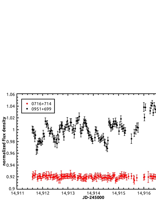
Figure 1: The variability curve (normalized flux density $S/\langle\,S\,\rangle$ versus time) of J0721+7120 (B0716+714, upper), together with a nearby secondary calibrator B0951+699 (lower) in epoch A. The offset of the two curves is arbitrary, for better visualization.

In addition, 11 sources have been measured for flux densities while they were not involved in the IDV observations, the flux densities are useful in the correlation analysis between radio flux density and $\it{Fermi}$ $\gamma$-ray intensity. So we list the source name/type (Q-quasar, BL-BL Lac object), flux density and observing epoch in Table 2, although three sources were measured for flux densities in July, August and September 2009. The radio galaxy 3C84 has the flux density of 16.174$\pm$0.065 Jy measured in March 9, 2009, which is not listed in Table 2.

Table 2: Flux densities measured for 10 blazars while they were not involved in IDV observations

Name/type	J0144+2705/BL	J0654+4514/Q	J0920+4441/Q	J0948+0022/Q	J1058+5628/BL
S(Jy)	0.240$\pm$0.003	0.449$\pm$0.003	1.058$\pm$0.006	0.191$\pm$0.006	0.189$\pm$0.007
Epoch	20090309	20090723	20090311	20090311	20090311
Name/type	J1229+0203/Q	J1253+5301/BL	J1542+6129/BL	J1959+6508/BL	J2325+3957/BL
S(Jy)	40.174$\pm$0.165	0.345$\pm$0.009	0.142$\pm$0.005	0.228$\pm$0.004	0.200$\pm$0.005
Epoch	20090311	20090311	20090919	20090309	20090819

4 Statistical analysis and results

For the data analysis, we use several quantities such as the modulation index, the variability amplitude and so forth. Here we just give a brief summary, a detailed description of these parameters can be found in Kraus et al. (2003).

1. The modulation index $m$

   $m$ is defined as the standard deviation of the flux density divided by the mean flux density of source.

   $$m[\%]=100\cdot\frac{\sigma_{S}}{\langle\,S\,\rangle},$$

   $m$ provides a measure of the strength of the variations observed. One should notice that it does not account for the intrinsic noise in the data.

2. The variability amplitude $Y$

   The noise-bias corrected variability amplitude $Y$ is defined as

   $$Y[\%]=3\sqrt{m^{2}-m_{0}^{2}},$$

   where $m_{0}$ is the mean modulation index of all non-variable sources (see Heeschen et al. 1987), so, it corresponds to the average residual noise and possibly even systematic scatter in the calibrators. Thus, compared to $m_{0}$, $Y$ works as a more uniform estimator of the variability strength, and it is useful for comparing data of different epochs.

3. $\chi^{2}$ and reduced $\chi^{2}$

   As a criterion for the source variability, the hypothesis of a constant function is examined and the calibrated data is fitted by a $\chi^{2}$ test of the kind

   $$\chi^{2}=\sum(\frac{S_{i}-\langle\,S\,\rangle}{\Delta\,S_{i}})^{2},$$

   with the reduced $\chi^{2}$

   $$\chi_{r}^{2}=\frac{1}{N-1}\cdot\sum(\frac{S_{i}-\langle\,S\,\rangle}{\Delta\,S_{i}})^{2},$$

   where $S_{i}$ denotes the individual flux densities, $\langle\,S\,\rangle$ their average in time, $\Delta\,S_{i}$ their errors and N the number of measurements (e.g. Bevington & Robertson 1992). Only those sources for which the probability that they can be fitted by a constant function is $\leq$ 0.1%, are considered to be variable.

We define the modulation index $M$ for the inter-month flux density variations similar as $m$ for the IDV. For the calibrators we obtain $M_{0}\sim$2 [%]. Because the inter-month data are sparse and unevenly sampled, we just treat the $M_{0}$ as the error of $M$, and did not define a noise-bias corrected $Y$ for the inter-month data.

Here, we present the basic information of the sources, and the statistical results of the IDV and inter-month observations at 4.8 GHz in Table LABEL:table:flux. The different columns are assigned as follows: column (1) source J2000 name; (2) optical identification (Q: quasar, BL: BL Lac object) and VLBI structure (c: extremely core dominated, cj: core with a mild jet); (3) the spectral index from the SPECFIND V2.0 catalog of broad band radio spectra (Vollmer et al. 2010), by using a least squares fit of the broad band [70-10500] MHz data for the majority of sources, and that the spectral index from two frequencies 1.4 and 8.4 GHz which is from the CRATES catalog (Combined Radio All-Sky Targeted Eight GHz Survey, Healey et al. 2007) except for three sources where the information is from NED; (4) symbols for different epochs (see Table 1); (5) effective number of flux measurements in IDV observation; (6) mean flux density in IDV observation; (7) the modulation index of IDV; (8) the reduced $\chi^{2}$ of IDV; (9) the variability amplitude of IDV, a zero is given if $m\leq m_{0}$; (10) IDV identification, a ‘$+$’ is given if the source shows IDV; (11) the mean flux density of the inter-month observations and the modulation index of inter-month variability; (12) the effective number of measurements for inter-month variability.

Table 3: The results of IDV and inter-month radio observations

Source	Id/vlbi	$\alpha 1^{0}/\alpha 2$	Ep	N	$\overline{S}$[Jy]	$m$[%]	$\chi_{r}^{2}$	$Y$[%]	IDV	$\overline{S_{M}}$[Jy]/$M$[%]	No.
(1)	(2)	(3)	(4)	(5)	(6)	(7)	(8)	(9)	(10)	(11)	(12)
J0112+2244	BL/c	0.18a/0.12	A	10	0.756	3.02	16.42	8.89	$+$	0.508/37.1	7
			B	10	0.674	6.21	30.56	18.51	$+$
J0136+4751	Q/c	0.10/0.19	A	13	4.320	1.18	9.93	3.04	$+$	4.044/6.6	8
J0217+0144	Q/c	0.16/0.24	A	7	1.298	2.17	12.74	6.24	$+$	1.284/7.0	7
			B	14	1.288	3.75	23.88	11.06	$+$
J0238+1636	BL/c	0.26/0.56	A	10	3.331	1.00	7.03	2.40	$+$	2.225/42.7	7
J0530+1331	Q/cj	0.44a/0.24	A	9	3.490	0.34	0.75	0.00		3.121/9.9	8
			B	15	3.587	2.95	34.38	8.61	$+$
J0654+5042	Q/cj	0.30a/0.23	A	9	0.315	1.57	1.23	4.37		0.313/10.2	7
			B	20	0.303	2.76	2.98	8.01	$+$
J0712+5033	BL/c	0.37a/0.40	A	12	0.313	2.79	4.13	8.17	$+$	0.315/9.4	2
			B	25	0.349	3.39	5.01	9.94	$+$
J0713+1935	Q/c	0.16b/0.35	A	9	0.276	6.81	17.04	20.34	$+$	0.254/19.1	2
			B	15	0.451	6.99	34.75	20.87	$+$
J0719+3307	Q/c	-0.20/-0.15	A	10	0.509	2.17	4.98	6.26	$+$	0.546/6.9	2
			B	24	0.595	3.83	13.53	11.30	$+$
J0721+7120	BL/c	-0.43c/-0.13	A	117	1.241	1.61	8.34	4.48	$+$	1.305/18.4	9
			B	92	1.361	3.66	37.68	10.77	$+$
			C	85	1.134	3.35	25.11	9.90	$+$
J0738+1742	BL/cj	-0.01/0.27	A	8	0.902	0.54	0.68	0.00		0.915/2.0	2
			B	16	0.935	2.75	14.26	7.97	$+$
J0818+4222	BL/cj	-0.10/-0.04	A	10	1.503	1.90	15.73	5.40	$+$	1.660/11.9	8
			B	24	1.522	2.03	8.07	5.71	$+$
J0824+5552	Q/cj	-0.08/0.10	A	13	1.049	0.59	0.92	0.00		1.083/6.7	7
			B	28	1.048	0.66	0.66	0.00
J0854+2006	BL/cj	0.35/0.44	A	8	1.952	1.56	12.16	4.31	$+$	1.911/5.1	2
J0957+5522	Q/cj	-0.34c/-0.41	A	13	1.939	0.15	0.08	0.00		1.980/4.6	8
			B	26	1.937	0.30	0.28	0.00
J1015+4926	BL/cj	-0.21/-0.24	A	10	0.358	1.48	1.15	4.04		0.352/4.0	4
			B	19	0.356	1.50	1.06	3.99
J1016+0513	Q/cj	-0.07a/-0.18	A	4	0.533	1.43	2.56	3.90		0.593/5.9	3
J1033+6051	Q/cj	-0.21c/-0.05	A	17	0.427	2.99	5.22	8.77	$+$	0.382/16.7	7
			B	34	0.412	2.89	4.61	8.41	$+$
J1104+3812	BL/cj	-0.25/-0.11	A	8	0.590	1.03	1.36	2.51		0.596/3.0	5
J1159+2914	Q/c	-0.29/-0.29	A	62	2.733	1.86	14.31	5.29	$+$	2.702/2.6	2
			B	55	2.627	1.30	4.69	3.29	$+$
J1217+3007	BL/cj	-0.33/-0.30	A	10	0.443	1.41	1.39	3.82		0.452/7.8	5
			B	19	0.441	1.55	1.54	4.13
J1221+2813	BL/cj	0.07/0.19	A	11	0.481	1.82	2.58	5.17		0.491/2.0	2
J1310+3220	Q/cj	0.09/0.30	A	9	1.054	2.00	7.06	5.73	$+$	1.222/8.7	6
			B	18	1.092	1.24	2.73	3.06	$+$
J1427+2348	BL/cj	-0.33/-0.34	A	10	0.362	2.20	2.38	6.36		0.340/1.5	3
			B	19	0.355	1.83	1.47	5.07
			C	2	0.359	1.16	0.27	2.96
J1504+1029	Q/cj	0.06/-0.03	A	8	1.524	0.63	0.77	0.54		1.601/8.2	9
			B	14	1.611	0.86	1.58	1.50
			C	31	1.725	0.94	1.98	2.17
J1522+3144	Q/c	-0.14/0.18	A	9	0.536	0.55	0.39	0.00		0.528/7.9	8
			C	33	0.512	2.60	4.61	7.60	$+$
J1553+1256	Q/cj	-0.26/-0.47	A	8	0.703	0.48	0.10	0.00		0.723/9.3	8
			C	29	0.721	1.37	2.40	3.71	$+$
J1555+1111	BL/c	0.04/0.26	C	13	0.315	2.79	1.46	8.18		0.298/4.8	4
J1635+3808	Q/cj	-0.01/-0.09	A	11	2.894	0.33	0.53	0.00		3.165/10.6	8
			B	21	2.931	0.38	0.55	0.00
			C	33	3.013	0.45	0.76	0.00
J1653+3945	BL/cj	-0.12/-0.19	A	10	1.535	0.58	0.95	0.00		1.573/7.7	8
			C	32	1.539	0.60	0.73	0.00
J1719+1745	BL/cj	0.21a/0.03	A	10	0.592	2.64	5.12	7.72	$+$	0.621/8.5	7
			B	19	0.590	1.77	3.16	4.87	$+$
			C	27	0.603	1.48	2.11	4.06	$+$
J1751+0939	BL/c	0.41a/0.64	A	10	2.872	1.37	9.51	3.69	$+$	3.204/16.8	3
			C	27	2.572	1.36	7.32	3.67	$+$
J1800+7828	BL/cj	0.07c/0.13	A	23	2.233	0.42	0.74	0.00		2.208/4.3	3
			B	42	2.128	0.50	0.68	0.00
			C	83	2.183	0.72	1.34	1.21
J1848+3219	Q/cj	-0.16a/0.11	A	9	0.557	1.73	2.83	4.87		0.619/8.2	3
			B	21	0.600	1.41	2.31	3.66	$+$
			C	30	0.623	1.15	1.48	2.93
J1849+6705	Q/c	-0.20c/-0.06	A	22	1.240	0.83	2.07	1.71		1.280/7.4	8
			B	40	1.272	1.79	7.69	4.95	$+$
			C	77	1.282	1.90	9.12	5.41	$+$
J2147+0929	Q/c	-0.09/0.03	A	11	0.782	2.25	7.83	6.49	$+$	0.983/16.3	5
			B	15	0.891	2.96	13.61	8.64	$+$
J2157+3127	Q/c	-0.16/0.07	A	7	0.399	1.19	1.03	3.09		0.480/17.5	7
J2202+4216	BL/cj	0.17/0.31	A	10	2.950	1.16	15.04	2.99	$+$	3.506/21.8	3
			B	24	3.125	0.57	1.25	0.00
J2203+1725	Q/c	0.00/0.32	A	12	1.022	2.15	14.05	6.21	$+$	0.972/5.0	2
			B	18	0.953	2.27	9.99	6.48	$+$
J2232+1143	Q/cj	-0.14/-0.42	A	7	4.605	0.53	1.48	0.00		4.794/2.4	2
			B	17	4.663	0.35	0.44	0.00
J2253+1608	Q/cj	-0.04/-0.11	A	12	10.417	0.54	2.11	0.00		10.390/6.1	7
J2327+0940	Q/cj	-0.03a/-0.08	A	7	1.372	9.35	125.19	27.98	$+$	1.379/2.5	2
			B	18	1.419	1.02	2.35	2.23

As shown in Table LABEL:table:flux, 26 sources (16 QSOs and 10 BL Lacs) show intra-day variability at a confidence level of larger than 99.9% at least once in IDV observations, according to $\chi^{2}$ test. Thus the IDV occurrence is 26 out of 42 $\it{Fermi}$-blazars, indicating the IDV detection rate is $\sim$60%, which is higher than that in previous flat-spectrum AGN samples (e.g. Quirrenbach et al. 1992; Lovell et al. 2008). This high rate could be caused by a higher compactness of $\it{Fermi}$ blazars relative to sources in other samples.

We find very pronounced inter-month variability in two BL Lac objects: J0112+2244 and J0238+1636, with modulation index 37.1% and 42.7%, respectively. Because the inter-month observation data are sparse and unevenly sampled, we will use only the 24 sources which have been observed at least in 5 months, for statistics in the following.

4.1 $\gamma$-ray and radio flux density

Combined radio and $\gamma$-ray data can be used to study the relationship between radio and $\gamma$-ray emission. We find that there is a correlation between the 4.8 GHz radio flux density of 52 sources and their $\gamma$-ray intensity (Fig. 2) with a Spearman correlation coefficient of 0.48 (significance 2.8$\times 10^{-4}$) in total, 0.37 (significance 0.06) for QSOs, and 0.61 (significance 0.001) for BL Lacs, respectively. For quasars the correlation seems not significant, especially when removing the two strong quasars 3C273 and 3C454.3. However there still has a correlation coefficient of 0.42 (significance 0.02) for 50 sources after dropping the 2 strong quasars. It is notable that our sample is incomplete and the radio-$\gamma$ data are not simultaneous. The 15 GHz simultaneous radio-$\gamma$ result obtained in Caltech group (Readhead, private communication) shows a more significant correlation, where a new Monte-Carlo method was applied and an intrinsic correlation was found (also see Ackermann et al. 2011).

The correlation between the radio and the $\gamma$-ray emission in the blazars can shed light on the physical link between the emission processes in the two energy bands. It is suggested that the $\it{Fermi}$-LAT detected blazars have on average higher Doppler factors than non-$\it{Fermi}$-LAT detected blazars (Savolainen et al. 2010). It is possible that the $\gamma$-ray emission (via synchrotron self-Compton and/or inverse-Compton scattering by the relativistic electrons in radio jet) from the $\it{Fermi}$-LAT detected blazars could also be Doppler-boosted.

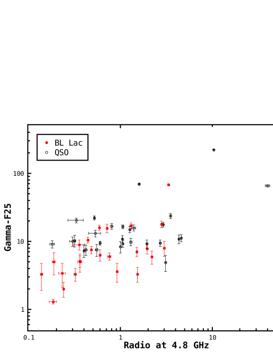
Figure 2: The mean flux densities (averaged over all IDV sessions) and those from Table 2 at 4.8 GHz vs. the gamma-ray intensities ($\geq$100 MeV, in $10^{-8}ph\,cm^{-2}s^{-1}$, from Abdo et al. 2009) of 52 $\it{Fermi}$-blazars; black: QSO, red: BL Lac.

4.2 Spectral index and flux density variability

It is possible that the 4.8 GHz flux density variability is related to the source spectral index. In order to obtain a more realistic estimate of the spectrum from broad-band radio data, we checked our 42 blazars in SPECFIND V2.0 catalog of broad band [30-10500] MHz radio continuum spectra (Vollmer et al. 2010), and obtained their indices, as the $\alpha 1$ shown in Table LABEL:table:flux. The frequency ranges of the spectra are [70-10500] MHz for 27 sources, [300-10500] MHz for 9 sources, [30-10500] MHz for 5 sources, and [1000-10000] MHz for 1 source, respectively. Although the spectral indices are from relatively low frequency ranges, the 42 blazars still show flat spectral indices $\alpha 1>-0.5$ from the SPECFIND V2.0 catalog. We also list the spectral index $\alpha 2$ calculated with 1.4 GHz and 8.4 GHz flux density from the CRATES catalog in Table LABEL:table:flux.

We plot the variability strength versus the spectral index for 42 blazars in Fig. 3. No obvious correlation was found between the spectral index $\alpha$ (from either the SPECFIND V2.0 catalog or the CRATES catalog) and variability amplitude $\langle\,Y\,\rangle$ of intra-day variability. The same results were obtained for inter-month variability (plot not shown here). However, it appears that the non-IDV blazars have the spectral indices $\alpha<0.1$ for the SPECFIND V2.0 and $\alpha<0.2$ (except one source with 0.26) for the CRATES 1.4/8.4 GHz spectral indices in Fig. 3, suggesting that the non-IDV blazars have relatively ‘steeper’ spectral indices than the IDV blazars in general.

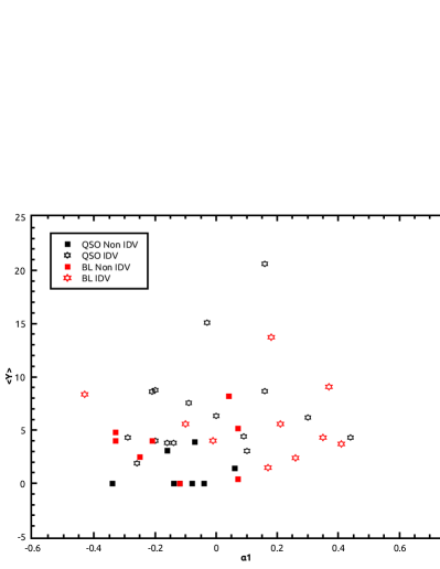
(a)

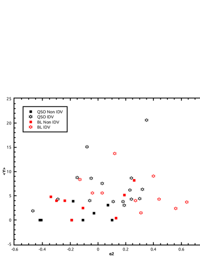
(b)

Figure 3: Intra-day variability amplitude $\langle\,Y\,\rangle$ (averaged over all IDV sessions, except when Y = 0) versus spectral index ($\alpha 1$ from SPECFIND V2.0 and $\alpha 2$ from CRATES); black: QSO, red: BL Lac; star: IDV, filled square: non-IDV.

4.3 IDV and inter-month variability

We tried to check whether there is a relationship between intra-day and inter-month variability. We use only the inter-month data which have been observed at least in 5 months. No significant correlation was found for the sub-sample of 24 sources, however, better results could be expected for more sophisticated observations on a larger sample of sources in future.

4.4 Variability strength of QSOs and BL Lacs

We studied the different variability strength $Y$ of IDV between QSOs and BL Lacs. Due to our incomplete sample, we calculate a median rather than a mean of the variability index. The result shows that the median is 3.96$\pm$4.92 for QSOs, and the median is 4.16$\pm$3.35 for BL Lacs. So there is no significant difference between QSO and BL Lac variability strength of IDV.

All the 42 sources have been observed by VLBI techniques, e.g. in MOJAVE project (Monitoring Of Jets in Active galactic nuclei with VLBA Experiments, see Lister et al. 2009), and in the VCS project (VLBA Calibrator Survey, http://astrogeo.org/vcs/). We roughly checked that the VLBI structures of the 42 blazars, found that 14 out of 16 the type ‘c’ blazars in Table LABEL:table:flux are IDV sources, suggesting that IDV occurs more often in the VLBI-core dominant blazars. There is no correlation between the IDV variability and the source redshift.

5 Summary and outlook

With the Urumqi telescope at 4.8 GHz, we have measured flux densities of 52 blazars, carried out IDV observations and inter-month flux monitoring for 42 blazars, from the first three-month $\it{Fermi}$-detected AGN list. We summary the results as follows:

1. 26 IDV sources are detected at a high confidence level, and the IDV detection rate of $\sim 60\%$ in the $\it{Fermi}$-blazar sample is higher than that in previous flat-spectrum AGN samples. The IDV appears more often in the VLBI-core dominant blazars.

2. There is a correlation between the 4.8 GHz radio flux density and the $\gamma$-ray intensity for the 42 blazars as a whole, in which the correlation confidence is higher for BL Lacs than that for quasars.

3. Pronounced inter-month variability was found in two BL Lac objects: J0112+2244 and J0238+1636.

4. No obvious correlation was found between the spectral indices and modulation indices of either intra-day or inter-month variability of the blazars. However, the non-IDV blazars tend to have relatively ‘steeper’ spectral indices than the IDV blazars in general.

5. No significant correlation between the intra-day and inter-month variability was found in the data.

6. No significant difference was found between QSO and BL Lac variability strength of IDV in the current sample.

We are aware of the fact that this sample is small. Following the pilot studies presented in this paper, we have launched a program to search for rapid variability in a large sample of radio sources with the Urumqi telescope in 2010, which uses the CRATES catalog as the parent sample to further investigate our findings. With this new project we plan to study in detail the statistics of IDV, a possible correlation between the occurrence of IDV and the presence of strong $\gamma$-ray emission, and the properties of $\gamma$-ray AGN and non-$\gamma$-ray AGN.

- (1) Abdo, A. A., Ackermann, M., Ajello, M. et al. 2010, ApJ, 715, 429
- (2) Abdo, A. A., Ackermann, M., Atwood, W. B., et al. 2009, ApJ, 700, 597
- (3) Ackermann, M., Ajello, M., Allafort, A., et al. 2011, arXiv:1108.0501
- (4) Baars, J. W. M., Genzel, R., Pauliny-Toth, I. I. K., Witzel, A. 1977, A&A, 61, 99
- (5) Benford, G. 1992, ApJ, 391, L59
- (6) Bevington, P. R., & Robinson, D. K. 1992, Data reduction and error analysis for the physical sciences (New York: McGraw-Hill)
- (7) Bignall, H. E., Jauncey, D. L., Lovell, J. E., et al. 2003, ApJ, 585, 653
- (8) Dennett-Thorpe, J., & de Bruyn, A. G. 2000, ApJ, 529, L65
- (9) Gabanyi, K. E., Marchili, N., Krichbaum, T. P., et al. 2009, A&A, 508, 161
- (10) Hartman, R. C., Bertsch, D. L., Bloom, S. D., et al. 1999, ApJS, 123, 79
- (11) Healey, S. E., Roger, Romani, R. W., Taylor, G. B., et al. 2007, ApJS, 171, 61
- (12) Heeschen, D. S., Krichbaum, T. P., Schalinski, C. J., & Witzel, A. 1987, AJ, 94, 1493
- (13) Kedziora-Chudczer, L., Jauncey, D. L., Wieringa, M. H., et al. 1997, ApJ, 490, L9
- (14) Kraus, A., Krichbaum, T.P., Wegner, R., et al. 2003, A&A, 401, 161
- (15) Kellermann, K. I., & Pauliny-Toth, I. I. K. 1969, ApJ, 155, L71
- (16) Lesch, H. & Pohl, M. 1992, A&A, 254, 29
- (17) Lister, M. L., Aller, H. D., Aller, M. F., et al. 2009, AJ, 137, 3718
- (18) Lovell, J. E. J., Rickett, B. J., Macquart, J.-P., et al. 2008, ApJ, 689, 108
- (19) Maraschi, L., Ghisellini, G., & Celotti, A. 1992, ApJ, 397, L5
- (20) Ott, M., Witzel, A., Quirrenbach, A., et al. 1994, A&A, 284, 331
- (21) Qian, S. -J., Li, X. -C., Wegner, R., et al. 1996, Chinese Astronomy and Astrophysics 20, 15
- (22) Quirrenbach, A., Witzel, A., Kirchbaum, T. P., et al. 1992, A&A, 258, 279
- (23) Readhead, A. C. S. 1994, ApJ, 426, 51
- (24) Rees, M. J. 1966, Nature, 211, 468
- (25) Savolainen, T., Homan, D. C., Hovatta, T. 2010, A&A, 512, A24
- (26) Sun, X. H., Han, J. L., Reich, W., et al. 2007, A&A, 463, 993
- (27) Urry, C. M., & Padovani, P. 1995, PASP, 107, 803
- (28) Vollmer, B., Gassmann, B., Derriere, S., et al. 2010, A&A,511, A53