Stationary distribution of a two-dimensional SRBM: geometric views and boundary measures

Abstract

We present three sets of results for the stationary distribution of a two-dimensional semimartingale reflecting Brownian motion (SRBM) that lives in the nonnegative quadrant. The SRBM data can equivalently be specified by three geometric objects, an ellipse and two lines, in the two-dimensional Euclidean space. First, we revisit the variational problem (VP) associated with the SRBM. Building on Avram, Dai and Hasenbein (2001), we show that the value of the VP at a point in the quadrant is equal to the optimal value of a linear function over a convex domain. Depending on the location of the point, the convex domain is either ${\cal D}^{(1)}$ or ${\cal D}^{(2)}$ or ${\cal D}^{(1)}\cap{\cal D}^{(2)}$, where each ${\cal D}^{(i)}$, $i=1,2$, can easily be described by the three geometric objects. Our results provide a geometric interpretation for the value function of the VP and allow one to see geometrically when one edge of the quadrant has influence on the optimal path traveling from the origin to a destination point. Second, we provide a geometric condition that characterizes the existence of a product form stationary distribution. Third, we establish exact tail asymptotics of two boundary measures that are associated with the stationary distribution; a key step in our proof is to sharpen two asymptotic inversion lemmas in Dai and Miyazawa (2011) that allow one to infer the exact tail asymptotic of a boundary measure from the singularity of its moment generating function.

1 Introduction

Multidimensional semimartingale reflecting Brownian motions (SRBMs) have been extensively studied in literature. They serve as diffusion models of multiclass queueing networks. See [16] for a survey on SRBMs and [17] on diffusion approximations. In this paper, we focus on a two-dimensional SRBM $Z=\{Z(t);t\geq 0\}$ that lives on the state space $\mathbb{R}_{+}^{2}$. We adopt the definition of an SRBM used in Dai and Miyazawa [5] and follow the notational system there. In particular, the data for the SRBM consists of a covariance matrix $\Sigma$, a drift vector $\mu$, and a reflection matrix $R$. They are written as

$$\mu=\left(\begin{array}[]{cc}\mu_{1}\\ \mu_{2}\end{array}\right),\qquad\Sigma=\left(\begin{array}[]{cc}\Sigma_{11}&\Sigma_{12}\\ \Sigma_{21}&\Sigma_{22}\end{array}\right),\qquad R=\left(\begin{array}[]{cc}r_{11}&r_{12}\\ r_{21}&r_{22}\end{array}\right).$$

In short, $Z$ is said to be a $(\Sigma,\mu,R)$-SRBM on $\mathbb{R}^{2}_{+}$. The covariance matrix $\Sigma$ and drift vector $\mu$ uniquely determine the following ellipse passing through the origin in $\mathbb{R}^{2}$:

$$\frac{1}{2}\left\langle\theta,\Sigma\theta\right\rangle+\left\langle\mu,\theta\right\rangle=0,\qquad\theta\in\mathbb{R}^{2},$$

where $\left\langle x,y\right\rangle$ denotes the usual inner product for vectors $x,y\in\mathbb{R}^{2}$ (see its definition at the end of this section). The first column $R^{1}$ of the reflection matrix $R$ determines a line, called line 1 in this paper, that passes through the origin and is orthogonal to direction $R^{1}$. In addition to the origin, the line intersects the ellipse at point $\theta^{(2,\rm r)}\neq 0$. Similarly, the second column $R^{2}$ of $R$ defines line 2 with intersection $\theta^{(1,\rm r)}\neq 0$ on the ellipse. These three geometric objects, the ellipse and two lines, uniquely determine the SRBM data $(\Sigma,\mu,R)$. See Figure 1 for an example of these three geometric objects and Section 3 for a precise definition of these objects. All results in this paper will have a geometric interpretation in terms of these three objects.

Throughout this paper, we assume conditions (2.1) and (2.2) in Section 2 on the SRBM data. These two conditions are necessary and sufficient for a two-dimensional SRBM to have a unique stationary distribution. Section 3.1 will give a geometric interpretation of these two conditions. In this paper, we present three sets of results for a two-dimensional SRBM. We first give a geometric interpretation for the value function of the variational problem that is associated with the SRBM. The value function has been conjectured to be the large deviations rate function of the stationary distribution. See inequalities (2.6), (2.7), and the text immediately following these inequalities for discussion on large deviations rate functions. We next give a geometric condition for the SRBM to have a product form stationary distribution. We finally present exact tail asymptotics of two boundary measures that are associated with the stationary distribution.

Closely related to the first set of our results, Avram et al. [1] studied the variational problem that is associated with a multidimensional SRBM. In the two-dimensional case, they obtained explicit expressions for the value function $I(v)$ for each point $v$ in the state space $\mathbb{R}^{2}_{+}$. In particular, they proved that $I(v)=\min(I^{(1)}(v),I^{(2)}(v))$, where $I^{(i)}(v)$ is the value function of a constrained variational problem with constrained path being restricted not to touch boundary

$$F_{i}=\{x\in\mathbb{R}^{2}_{+}:x_{i}=0\}$$

of the state space, $i=1,2$. To compute $I^{(i)}(v)$, they showed that an optimal path from the origin to $v$ is either a straight line through the interior of the state space or a broken path whose first segment travels on boundary $F_{3-i}$. In either case, they give an explicit algebraic expression for $I^{(i)}(v)$. Central in their analysis is a notion of “exit velocity” that dictates the direction for the broken path to follow when it exits the boundary $F_{3-i}$. Theorem 3.1 and Lemma 3.2 of this paper give a geometric interpretation of $I^{(i)}(v)$. In particular, we show that the exit velocity $\tilde{a}^{1}$ on boundary $F_{1}$ and the exit velocity $\tilde{a}^{2}$ on boundary $F_{2}$ have the following expressions

$$\tilde{a}^{1}=n^{\Gamma}(\tilde{\theta}^{(2,r)})\quad\text{ and }\quad\tilde{a}^{2}=n^{\Gamma}(\tilde{\theta}^{(1,r)}),$$ (1.2)

respectively, where $n^{\Gamma}(\theta)$, defined in (3.18) in Section 3, is the normal direction of the ellipse at point $\theta$ on the ellipse and $\tilde{\theta}^{(i,r)}$ is the “symmetry” of $\theta^{(i,\rm r)}$ on the ellipse; see Figure 6 for an illustration of $n^{\Gamma}(\theta)$ and Figure 3 for an illustration of symmetry points. Theorem 3.2 gives a geometric interpretation of $I(v)$. Harrison and Hasenbein [8] re-express the solution in [1] for $I(v)$ in an alternative form that is somewhat more explicit, and offer further elaboration on the structure of that solution.

A key step in our analysis is to connect the variational problem with the optimization problems of a linear function over certain convex domains. Those convex domains are closely related to the convergence domain of the two-dimensional moment generating function of the stationary distribution. Dai and Miyazawa [5] studied the exact tail asymptotics of the stationary marginal distribution for the two dimensional SRBM. In particular, they characterized the convergence domain through the three geometric objects. In this paper, we show that the convergence domain is the intersection of two convex domains and the rate function $I(v)$ can be uniquely determined by these two convex domains. Each of these convex domains can easily be determined by the three geometric objects. In this way, we provide a geometric interpretation of the large deviations rate function $I(v)$ (see Theorems 3.1 and 3.2).

Our second set of results is to characterize geometrically the existence of the product form stationary distribution. We prove in 5.1 that the stationary distribution of a two-dimensional SRBM has a product form if and only if

$$\tilde{\theta}^{(1,\rm r)}=\tilde{\theta}^{(2,\rm r)}.$$

See Figure 9 for examples. This geometric characterization contrasts with the algebraic characterization developed in Harrison and Williams [10]. Their characterization, in terms of a skew symmetry condition, is valid for an SRBM in an arbitrary dimension.

Our last set of results (Theorem 6.1) concerns the exact tail asymptotics for two boundary measures $\nu_{1}$ and $\nu_{2}$ that are associated with the stationary distribution. This set of results is closely related to the recent paper [5] in which moment generating functions are used to obtain the exact tail asymptotic for stationary marginal distributions. Their analysis relies on two asymptotic inversion lemmas to obtain the exact tail asymptotics from the singularity of the moment generating functions. Unfortunately, these inversion lemmas are not sharp enough for us to study exact tail asymptotics for boundary measures. In this paper, we develop a series of three lemmas, Lemmas 6.1, 6.2 and 6.3, to sharpen the asymptotic inversion lemmas. These lemmas should also be useful for other problems; see Section 6 for more discussions.

This paper consists of six sections. In Section 2, we discuss the variational problem of an SRBM and its relation to the large deviations rate function for the stationary distribution. In Section 3, we first define three geometric objects and two convex domains ${\cal D}^{(1)}$ and ${\cal D}^{(2)}$. We then state the first set of results, Theorems 3.1 and 3.2. In Section 4, we review some results in Avram et al. [1] and prove Theorem 3.1. In Section 5, we give a geometric characterization for the existence of a product form stationary distribution. In Section 6, we study exact tail asymptotics of two boundary measures. In the rest of this section, we summarize the notation used in this paper for the convenience of readers.

Notation: Let $\mathbb{R}$ and $\mathbb{C}$ be the sets of all real and complex numbers, respectively, and let $\mathbb{R}_{+}$ be the set of all nonnegative real numbers. All vectors are envisioned as column vectors, and $x^{{\mbox{\scriptsize\sc t}}}$ is the transpose of vector $x$. In this paper, we adopt the standard inner product, that is,

$$\left\langle x,y\right\rangle=x^{{\mbox{\scriptsize\sc t}}}y\quad\text{ for }x,y\in\mathbb{R}^{2}$$

with the corresponding standard norm $\|x\|=\sqrt{\left\langle x,x\right\rangle}$ for each $x\in\mathbb{R}^{2}$. We list the notation for the primitive data and the stationary distribution of SRBM in Tables 1 and 2 below.

Table 1: Notation associated with the primitive data ($i=1,2$)

$\mu$	drift vector of SRBM	$\Sigma$	covariance matrix of SRBM
$R$	reflection matrix	$R^{i}$	the $i$-th column of $R$
$\gamma(\theta)$	$-\frac{1}{2}\left\langle\theta,\Sigma\theta\right\rangle-\left\langle\mu,\theta\right\rangle$ for $\theta\in\mathbb{R}^{2}$	$\gamma_{i}(\theta)$	$\left\langle R^{i},\theta\right\rangle$ for $\theta\in\mathbb{R}^{2}$
$\Gamma$	$\{\theta\in\mathbb{R}^{2};\gamma(\theta)>0\}$	$\Gamma_{i}$	$\{\theta\in\Gamma;\gamma_{3-i}(\theta)<0\}$
$\partial\Gamma$	$\{\theta\in\mathbb{R}^{2};\gamma(\theta)=0\}$	$\partial\Gamma_{i}$	$\{\theta\in\Gamma;\gamma_{3-i}(\theta)=0\}$
$\Gamma_{\max}$	$\{\theta\in\mathbb{R}^{2};\exists\,\theta^{\prime}\in\Gamma,\theta<\theta^{\prime}\}$	$\theta^{(i,\max)}$	$\arg\max_{\theta\in\partial\Gamma}\theta_{i}$
$\theta^{(i,{\rm r})}$	the nonzero intersection	$\tilde{\theta}^{(i,{\rm r})}$	$\theta^{(i,\max)}$ if $\theta^{(i,{\rm r})}=\theta^{(i,\max)}$,
	of $\gamma(\theta)=0$ and $\gamma_{3-i}(\theta)=0$		otherwise, $\theta$ on $\partial\Gamma$ such that
			$\theta_{i}=\theta^{(i,{\rm r})}_{i}$ and $\theta_{3-i}\neq\theta^{(i,{\rm r})}_{3-i}$
$\theta^{(i,\Gamma)}$	$\arg\max_{\theta\in\partial\Gamma_{i}}\theta_{i}$	$\theta^{(v,\Gamma)}$	$\arg\max_{\theta\in\partial\Gamma}\left\langle v,\theta_{i}\right\rangle$ for $v\in\mathbb{R}_{+}^{2}$
$p^{(i)}$	the $i$-th row of $(\det{R})R^{-1}$	${\rm n}^{\Gamma}(\theta)$	$\Sigma\theta+\mu$
$a^{i}$	${\rm n}^{\Gamma}(\theta^{(3-i,{\rm r})})$	$\tilde{a}^{i}$	${\rm n}^{\Gamma}(\tilde{\theta}^{(3-i,{\rm r})})$

Let $Z(\infty)$ be a random variable following the stationary distribution $\pi$ of the SRBM, and let $\nu_{i}$ be the measure on the boundary face $F_{3-i}\equiv\{x\in\mathbb{R}_{+}^{2};x_{3-i}=0\}$ associated with $\pi$ as defined in Section 2 of [5].

Table 2: Notation associated with the stationary distribution of SRBM $(i=1,2)$

$\varphi(\theta)$	$\mathbb{E}(e^{\left\langle\theta,Z(\infty)\right\rangle})$	$\varphi_{i}(\theta_{3-i})$	the moment generating function of $\nu_{i}$
${\cal D}$	the interior of $\{\theta\in\mathbb{R}^{2};\varphi(\theta)<\infty\}$	${\cal D}^{(i)}$	$\{\theta\in\mathbb{R}^{2};\exists\,\theta^{\prime}\in\Gamma,\theta<\theta^{\prime},\theta^{\prime}_{i}<\theta_{i}^{(i,\Gamma)}\}$
$\tau_{i}$	$\sup\{\theta_{i}>0;\theta\in{\cal D}\}$	${\rm e}^{(i)}$	the unit vector for the $i$-th axis
${\rm e}^{i}$	${\rm e}^{(3-i)}$	${\rm n}^{i}$	${\rm e}^{(i)}$
$\zeta$	the joint density of $\pi$	$\zeta_{i}$	the marginal density of $\pi$
VP	variational problem	$I(v)$	the value function of VP

2 Variational problem and large deviations principle

In Section 4, we recover results obtained by Avram et al. [1], leveraging recent results of Dai and Miyazawa [5]. Those two papers use different sets of notation. For example, Avram et al. [1] used $\Gamma$ for covariance matrix and $\theta$ for drift vector instead of $\Sigma$ and $\mu$ in this paper. Furthermore, $R$ in [1] is normalized in such a way that $r_{11}=r_{22}=1$. Following [5], we will not use any normalization in this paper. In Avram et al. [1], the inner product $\left\langle x,y\right\rangle$ for vectors $x,y\in\mathbb{R}^{2}$ is defined as $x^{{\mbox{\scriptsize\sc t}}}\Sigma^{-1}y$. Their inner product certainly simplifies computation, but is also potentially confusing because there is no indication of $\Sigma^{-1}$.

As in [5], we assume that $\Sigma$ is non-singular and the SRBM data $(\Sigma,\mu,R)$ satisfy

$$r_{11}>0,\quad r_{22}>0,\quad r_{11}r_{22}-r_{12}r_{21}>0,$$ (2.1)

$$r_{22}\mu_{1}-r_{12}\mu_{2}<0,\quad r_{11}\mu_{2}-r_{21}\mu_{1}<0.$$ (2.2)

Under conditions (2.1) and (2.2), the $(\Sigma,\mu,R)$-SRBM is well defined, and its stationary distribution exists and is unique; see, for example, [8, 11].

We are going to introduce the variational problem associated with the SRBM shortly. For that, we first define the Skorohod problem associated with the reflection matrix $R$. Let $\mathbb{D}^{2}=\mathbb{D}(\mathbb{R}_{+},\mathbb{R}^{2})$ be the set of functions from $\mathbb{R}_{+}$ to $\mathbb{R}^{2}$ that are right continuous on $[0,\infty)$ and have left limits in $(0,\infty)$. Assume that the reflection matrix $R$ satisfies condition (2.1). Then, $R$ is a completely-${\cal S}$ matrix (for a definition see, for example, the second paragraph of the introduction in [5]). Therefore, for each $x(\cdot)\in\mathbb{D}^{2}$, there exists a $z(\cdot)\in\mathbb{D}^{2}$ such that $z(\cdot)$, together with some $y(\cdot)\in\mathbb{D}^{2}$, satisfies the following three conditions

$$z(t)=x(t)+Ry(t)\geq 0,\qquad t\geq 0,$$ (2.3)

$$y(0)=0\text{ and each component of $y$ is non-decreasing},$$ (2.4)

$$\int_{0}^{\infty}z_{i}(t)dy_{i}(t)=0,\quad i=1,2.$$ (2.5)

The path $z$ is called an $R$-regulation of $x$. It is not unique in general (e.g., see [12]). Conditions (2.3)-(2.5) define the Skorohod problem associated with $R$.

Assume conditions (2.1) and (2.2) so that the stationary distribution is uniquely determined. Let $Z(\infty)$ be a random vector whose distribution is the stationary distribution. If there is a lower semi-continuous function $I(\cdot)$ from $\mathbb{R}_{+}^{2}$ to $\mathbb{R}_{+}$ that satisfies

$$\limsup_{u\to\infty}\frac{1}{u}\log\mathbb{P}(Z(\infty)\in uB)\leq-\inf_{v\in\overline{B}}I(v),$$ (2.6)

$$\liminf_{u\to\infty}\frac{1}{u}\log\mathbb{P}(Z(\infty)\in uB)\geq-\inf_{v\in B^{\rm o}}I(v)$$ (2.7)

for any measurable $B\subset\mathbb{R}_{+}^{2}$, where $\overline{B}$ and $B^{\rm o}$ are closure and interior of $B$, respectively, it is said that the large deviations principle (LDP) holds for the stationary distribution, and $I(v)$ is called a large deviations rate function.

The LDP for the stationary distribution is verified by Majewski [13, Theorem 4] for a multidimensional SRBM whose reflection matrix $R$ is an ${\cal M}$ matrix and the stability condition $R^{-1}\mu<0$ holds. Specializing his result to two dimensions, we see that, under condition (2.1), $R^{-1}\mu<0$ is equivalent to (2.2). Furthermore, again specializing to two-dimensional case, for each $v\in\mathbb{R}_{+}^{2}$, he identifies the rate function $I(v)$ as the value function of the following variational problem (VP)

$$I(v)=\inf_{T\geq 0}\inf_{x\in{\cal H},z(T)=v}\frac{1}{2}\int_{0}^{T}\langle\dot{x}(t)-\mu,\Sigma^{-1}(\dot{x}(t)-\mu)\rangle dt,$$ (2.8)

where each $x(\cdot)\in{\cal H}\subset\mathbb{D}^{2}$ is an absolutely continuous function on $\mathbb{R}_{+}$ such that its derivative function is locally square integrable with respect to the Lebesgue measure, and $z(\cdot)\in\mathbb{D}^{2}$ is an $R$-regulation of $x(\cdot)$. In general, an $R$-regulation $z$ in (2.8) is not unique, and the inner inf is taken over all such $z$. Dupuis and Ramanan [7] proved an LDP when the ${\cal M}$ matrix condition in [13] was relaxed. However, an LDP for a general SRBM remains unproven. Despite the lack of such a general LDP, the VP (2.8) is well defined for a general SRBM. The focus of this paper is VP (2.8). We use terms value function of the VP and large deviations rate function interchangeably even though the latter term does not make sense when the corresponding LDP has not been proven.

For two-dimensional SRBMs, Avram et al. [1] solved VP (2.8) completely. In particular, they proved that the value $I(v)$ of (2.8) can be obtained by restricting paths $x$ to one of the three types. For each $T>0$ and $v\in\mathbb{R}_{+}^{2}$, define ${\cal H}^{(0)}(v,T)$ to be the set of linear paths $x\in\mathbb{D}^{2}$ from $0$ to $v$ such that $x(T)=v$. Define ${\cal H}^{(1)}(v,T)$ to be the set of continuous paths $x$ that have two linear segments: during the first segment, a regulated path $z$ of $x$ stays on the boundary $F_{2}$ of the state space $\mathbb{R}^{2}_{+}$ and during the second segment, the regulated path travels linearly from the boundary to the end point $v$ at time $T$. Namely,

$${\cal H}^{(1)}(v,T)=\biggl{\{}x\in{\cal H};x(t)=tc\text{ for }t\in[0,s]\text{ and }x(t)=\frac{t-s}{T-s}(v-z(s))+sc\text{ for }$$

$$\hskip 47.36096ptt\in(s,T]\text{ for some }s\in[0,T)\text{ and some }c\in\mathbb{R}^{2}\text{ with }c_{1}>0\text{ and }c_{2}<0\biggr{\}}.$$

Similarly, define ${\cal H}^{(2)}(v,T)$ to be the set of two segment paths so that during the first segment, an regulated path $z$ stays on boundary $F_{1}$ of the state space.

Using these sets, let

$$I^{(i)}(v)=\inf_{T>0}\inf_{x\in{\cal H}^{(i)}(v,T),z(T)=v}\frac{1}{2}\int_{0}^{T}\langle\dot{x}(t)-\mu,\Sigma^{-1}(\dot{x}(t)-\mu)\rangle dt,\qquad i=0,1,2.$$ (2.9)

Remark 2.1.

We here slightly changed the notation of Avram et al. [1]. Namely, $I^{(1)}(v)$ and $I^{(2)}(v)$ are $\tilde{I}^{2}(v)$ and $\tilde{I}^{1}(v)$ of [1], respectively, while $I^{(0)}(v)$ is the same as $\tilde{I}^{0}(v)$ in [1].

We now present the following well known fact (see Theorem 5.1 of Avram et al. [1] for its proof).

Lemma 2.1.

For an SRBM that satisfies (2.1) and (2.2), the rate function $I(v)$ is obtained as

$$I(v)=\min(I^{(1)}(v),I^{(2)}(v)),\qquad v\in\mathbb{R}_{+}^{2}.$$ (2.10)

Remark 2.2.

$I(v)$ is often written as

$$I(v)=\min(I^{(0)}(v),I^{(1)}(v),I^{(2)}(v)),\qquad v\in\mathbb{R}_{+}^{2}.$$

However, ${\cal H}^{(0)}\subset{\cal H}^{(1)}\cap{\cal H}^{(2)}$, and therefore (2.10) is also valid.

Avram et al. [1] explicitly obtained expressions for $I(v)$ in (2.10) in their Theorem 3.1 and Lemma 6.1. However, it is difficult to see how the rate function $I(v)$ depends on the SRBM data $(\Sigma,\mu,R)$ from their results. In the next section, we use a geometric method to compute $I(v)$ directly. In Section 4 we will show that the computation in Section 3 recovers the results in [1].

3 Geometrical view

Recall that $Z(\infty)$ is the random vector whose distribution is the stationary distribution of the two-dimensional SRBM. Denote the moment generating function of $Z(\infty)$ by $\varphi$, that is,

$$\varphi(\theta)=\mathbb{E}\left(e^{\left\langle\theta,Z(\infty)\right\rangle}\right),\quad\text{ for }\theta\in\mathbb{R}^{2}$$ (3.1)

as long as $\varphi(\theta)<\infty$. Dai and Miyazawa [5] identified the convergence domain ${\cal D}$, which is defined to be

$${\cal D}=\mbox{the interior of }\{\theta\in\mathbb{R}^{2};\varphi(\theta)<\infty\}.$$

In this paper, we provide an alternative characterization of the convergence domain ${\cal D}$; see Theorem 3.2 below in this section. The characterization allows us to compute the value functions $I^{(1)}(v)$ and $I^{(2)}(v)$ geometrically for variational problem (2.9)

3.1 SRBM data and conditions for existence and stability

To describe the convergence domain ${\cal D}$ and its alternative characterization, we first introduce three functions on $\mathbb{R}^{2}$. They are

$$\gamma(\theta)=-\frac{1}{2}\left\langle\theta,\Sigma\theta\right\rangle-\left\langle\mu,\theta\right\rangle,$$ (3.2)

$$\gamma_{i}(\theta)=\langle R^{i},\theta\rangle=\theta_{1}r_{1i}+\theta_{2}r_{2i},\qquad i=1,2,$$ (3.3)

where $R^{i}$ is again the $i$th column of the reflection matrix $R$. These three functions determine three geometric objects on the plane $\mathbb{R}^{2}$. Because we assume $\Sigma$ is nondegenerate, the quadratic equation $\gamma(\theta)=0$ determines an ellipse that passes through the origin. Two linear equations $\gamma_{1}(\theta)=0$ and $\gamma_{2}(\theta)=0$ determine two lines that pass through the origin. See Figure 1 for an example.

Let

$$p^{(1)}=\left(\begin{array}[]{c}r_{22}\\ -r_{12}\end{array}\right),\qquad p^{(2)}=\left(\begin{array}[]{c}-r_{21}\\ r_{11}\end{array}\right).$$

One can check that the transpose of $p^{(i)}$ is the $i$th row of the matrix $R^{-1}\det(R)$, where $\det(R)$ is the determinant of $R$. Thus, $p^{(1)}$ and $p^{(2)}$ are orthogonal to the second and first columns, respectively, of $R$. Note that $p^{(1)}=p^{2}$ and $p^{(2)}=p^{1}$, where $p^{i}$ is defined in [1] for $i=1,2$. Clearly, line $\gamma_{1}(\theta)=0$ parallels directional vector $p^{(2)}$ and line $\gamma_{2}(\theta)=0$ parallels directional vector $p^{(1)}$. It is convenient to assign a direction for each line and from now on a directional line is called a ray. We assume ray $\gamma_{1}(\theta)=0$ points in the direction of $p^{(2)}$ and ray $\gamma_{2}(\theta)=0$ points in the direction of $p^{(1)}$. In Figure 1, these directions are denoted by arrows on two lines.

Specifying the three geometric objects in Figure 1 is equivalent to specifying the SRBM data $(\Sigma,\mu,R)$.

Figure 1: Specifying the SRBM data $(\Sigma,\mu,R)$ is equivalent to specifying an ellipse and two rays, all passing through the origin. The ellipse has normal direction $\mu$ at the origin. Ray $\gamma_{3-i}(\theta)=0$ has direction $p^{(i)}$ that intersects with the ellipse at a point $\theta^{(i,r)}\neq 0$, $i=1,2$. Stability condition (3.5) is satisfied for the left figure and not satisfied for the right figure

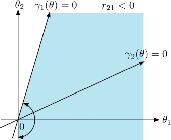
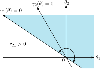
Figure 2: The ${\cal P}$ matrix condition (2.1) is equivalent to that ray $\gamma_{2}(\theta)=0$ must lie in the shaded region

A ray passing through the origin can be uniquely determined by its angle in $(-\pi,\pi]$, measured counter-clockwise against the $\theta_{1}$ axis; the angle is positive if the ray points above the axis, and is negative if it points below the axis. Ray one is said to be above (below) ray two if angle one is strictly larger (smaller) than angle two. Ray one is said to be on ray two if the two angles are equal.

Geometrically, the ${\cal P}$ matrix condition (2.1) is equivalent to ray $\gamma_{2}(\theta)=0$ being below ray $\gamma_{1}(\theta)=0$; see Figure 2 for an example. With the definition of $p^{(i)}$ for $i=1,2$, the stability condition (2.2) can be written as

$$\left\langle\mu,p^{(1)}\right\rangle<0,\quad\left\langle\mu,p^{(2)}\right\rangle<0.$$ (3.5)

As discussed in [5], this is an important observation in the geometrical view of the stability condition. Condition (3.5) is equivalent to the angle between vector $\mu$ and each ray being more than $\pi/2$. In Figure 1, the left panel corresponds a stable SRBM and the right panel an unstable SRBM. Since $\mu$ is the normal direction of the ellipse at the origin, condition (3.5) ensures that ray $\gamma_{i}(\theta)=0$ is not tangent to the ellipse, and therefore it must intersect with the ellipse at a point other than the origin.

3.2 Convergence domain and rate function

Let

$$\Gamma=\{\theta\in\mathbb{R}^{2};\gamma(\theta)>0\}$$

denote the interior of the ellipse. Its boundary $\partial\Gamma$ is the ellipse itself. Since $\gamma(\theta)$ is a convex function, $\Gamma$ is a convex set. We use $\theta^{(1,\max)}$ to denote the right-most point on $\partial\Gamma$ and $\theta^{(2,\max)}$ the highest point; namely,

$$\theta^{(i,\max)}=\arg\max_{\theta\in\partial\Gamma}\theta_{i},\quad i=1,2.$$

We also define two subsets $\Gamma_{1}$ and $\Gamma_{2}$ of $\Gamma$ via

$$\Gamma_{i}=\{\theta\in\Gamma;\gamma_{3-i}(\theta)<0\}\quad\text{ for }i=1,2.$$ (3.6)

Clearly, $\Gamma_{1}$ is the region inside the ellipse and is below ray $\gamma_{2}(\theta)=0$ and $\Gamma_{2}$ is the region inside the ellipse and is above ray $\gamma_{1}(\theta)=0$. Similar to $\partial\Gamma$, the boundary of $\Gamma_{i}$ is denoted by $\partial\Gamma_{i}$ for $i=1,2$. Following [5], we use $\theta^{(1,\rm r)}$ to denote the intersection of ray $\gamma_{2}(\theta)=0$ with the ellipse (other than the origin), and $\theta^{(2,\rm r)}$ the intersection of ray $\gamma_{1}(\theta)=0$ with the ellipse; see Figure 1. We note that $\theta^{(1,\rm r)}$ is proportional to $p^{(1)}$ and therefore $\theta^{(1,\rm r)}_{1}p^{(1)}=r_{22}\theta^{(1,\rm r)}$. Hence, $\gamma(\theta^{(1,\rm r)})=0$ implies that

$$\theta^{(1,\rm r)}_{1}=-\frac{2r_{22}\left\langle\mu,p^{(1)}\right\rangle}{\left\langle p^{(1)},\Sigma p^{(1)}\right\rangle}\quad\text{ and }\quad\theta^{(1,\rm r)}_{2}=\frac{2r_{12}\left\langle\mu,p^{(1)}\right\rangle}{\left\langle p^{(1)},\Sigma p^{(1)}\right\rangle}.$$

One can similarly compute $\theta^{(2,\rm r)}_{1}$ and $\theta^{(2,\rm r)}_{2}$. Thus, we have

$$\theta^{(i,r)}=-\frac{2\left\langle\mu,p^{(i)}\right\rangle}{\left\langle p^{(i)},\Sigma p^{(i)}\right\rangle}p^{(i)},\quad i=1,2.$$ (3.7)

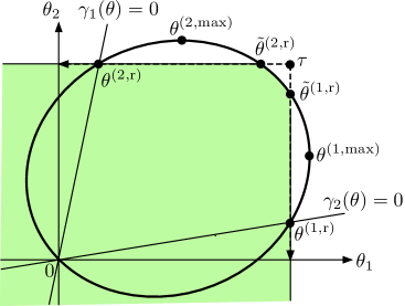
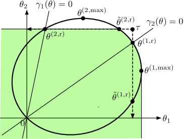
Figure 3: Three pairs of points: $\theta^{(i,r)}$, $\tilde{\theta}^{(i,r)}$ and $\theta^{(i,\max)}$ on the ellipse

Condition (2.2) or condition (3.5) is equivalent to

$$\theta^{(i,r)}_{i}>0\quad\text{ for }i=1,2.$$ (3.8)

Now we define a pair of points $\tilde{\theta}^{(1,\rm r)}$ and $\tilde{\theta}^{(2,\rm r)}$ on $\partial\Gamma$. The point $\tilde{\theta}^{(1,\rm r)}$ is defined to be the “symmetry” of $\theta^{(1,r)}$ on $\partial\Gamma$. When $\theta^{(1,\rm r)}=\theta^{(1,\max)}$, we define $\tilde{\theta}^{(1,\rm r)}$ to be $\theta^{(1,\max)}$ itself. When $\theta^{(1,\rm r)}\neq\theta^{(1,\max)}$, we define $\tilde{\theta}^{(1,\rm r)}$ to be the unique point on $\partial\Gamma$ such that

$$\tilde{\theta}^{(1,r)}_{1}=\theta^{(1,\rm r)}_{1}\quad\text{ and }\quad\tilde{\theta}^{(1,r)}_{2}\not=\theta^{(1,\rm r)}_{2}.$$ (3.9)

Similarly, we can define $\tilde{\theta}^{(2,\rm r)}$. See Figure 3 for examples of three pairs of points $\theta^{(i,r)}$, $\tilde{\theta}^{(i,r)}$ and $\theta^{(i,\max)}$, $i=1,2$. As illustrated in the figure, $\tilde{\theta}^{(1,\rm r)}$ can be higher or lower than $\theta^{(1,\rm r)}$.

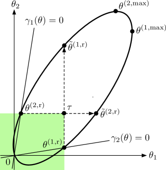
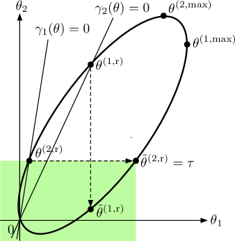
Figure 4: An example in which both $\theta^{(1,\rm r)}$ and $\tilde{\theta}^{(1,\rm r)}$ are lower than $\theta^{(1,\max)}$

The following is an important condition for the SRBM data:

$$\theta^{(1,\max)}\in\partial\Gamma_{1}$$ (3.10)

In the right panel of Figure 3, condition (3.10) is satisfied, while in the left panel, the condition is not satisfied. As it will be explained in Section 4, condition (3.10) is equivalent to the fact that the face $F_{2}=\{x\in\mathbb{R}^{2}_{+};x_{2}=0\}$ is not reflective, an important term introduced in [1]. Its meaning is explained in [1, page 264]; “When $F_{i}$ is not reflective, …, the face $F_{i}$ has no boundary influence on solutions to the VP [in (2.8)] for any $v\in\mathbb{R}^{2}_{+}$”.

Under condition (3.10), $\tilde{\theta}^{(1,\rm r)}$ is always at most as high as $\theta^{(1,\rm r)}$. Readers are warned that condition (3.10) is not equivalent to

$$\theta^{(1,\rm r)}_{2}\geq\theta^{(1,\max)}_{2}.$$ (3.11)

The right panel of Figure 4 gives an example that satisfies condition (3.10), but not condition (3.11). Conditions (3.10) and (3.11) are equivalent if and only if $\theta^{(1,\rm r)}$ or $\tilde{\theta}^{(1,\rm r)}$ is on the right side of $\theta^{(2,\max)}$, namely,

$$\theta^{(1,\rm r)}_{1}=\tilde{\theta}^{(1,\rm r)}_{1}\geq\theta^{(2,\max)}_{1}.$$ (3.12)

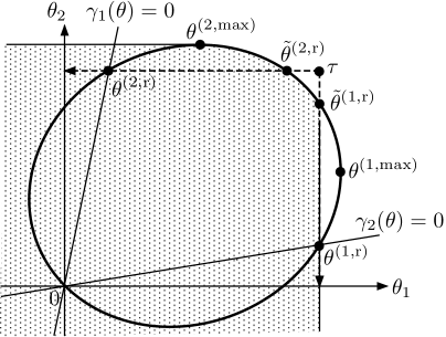
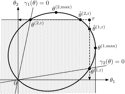
Figure 5: An example of ${\cal D}^{(1)}$ (left) and ${\cal D}^{(2)}$ (right)

Now we define two subsets ${\cal D}^{(1)}$ and ${\cal D}^{(2)}$ of $\mathbb{R}^{2}$. For this, the following points on the ellipse $\partial\Gamma$ are convenient:

$$\theta^{(i,\Gamma)}=\left\{\begin{array}[]{ll}\theta^{(i,\rm r)},&\mbox{if }\theta^{(i,\max)}\not\in\partial\Gamma_{i},\\ \theta^{(i,\max)},&\mbox{if }\theta^{(i,\max)}\in\partial\Gamma_{i},\end{array}\right.\qquad i=1,2.$$

We define

$${\cal D}^{(i)}=\Bigl{\{}\theta\in\mathbb{R}^{2};\text{ there exists a }\theta^{\prime}\in\Gamma\text{ such that }\theta<\theta^{\prime}\text{ and }\theta_{i}^{\prime}<\theta^{(i,\Gamma)}_{i}\Bigr{\}},\quad i=1,2.$$ (3.14)

In what follows, we mainly consider ${\cal D}^{(1)}$ because results for ${\cal D}^{(2)}$ are symmetric. Note that the definition of ${\cal D}^{(1)}$ depends on whether condition (3.10) is satisfied. We have the following lemma.

Lemma 3.1.

The domain ${\cal D}^{(1)}$ has the following form:

$${\cal D}^{(1)}=\begin{cases}\bigl{\{}\theta\in\mathbb{R}^{2};\theta<\tilde{\theta}^{(1,\rm r)}\bigr{\}}&\mbox{if }\theta^{(1,\max)}\not\in\partial\Gamma_{1}\mbox{ and if }\theta^{(1,\rm r)}_{1}\leq\theta^{(2,\max)}_{1},\\ \Gamma_{\max}\cap\bigl{\{}\theta\in\mathbb{R}^{2};\theta_{1}<\tilde{\theta}^{(1,\rm r)}_{1}\bigr{\}}&\mbox{if }\theta^{(1,\max)}\not\in\partial\Gamma_{1}\mbox{ and if }\theta^{(1,\rm r)}_{1}>\theta^{(2,\max)}_{1},\\ \Gamma_{\max},&\text{if }\theta^{(1,\max)}\in\partial\Gamma_{1},\end{cases}$$ (3.15)

where

$$\Gamma_{\max}=\{\theta\in\mathbb{R}^{2};\text{ there exists a $\theta^{\prime}\in\Gamma$ such that $\theta<\theta^{\prime}$}\}.$$ (3.16)

Proof.

Assume that condition (3.10) is satisfied. Then, $\theta^{(1,\Gamma)}=\theta^{(1,\max)}$, and therefore ${\cal D}^{(1)}=\Gamma_{\max}$ (see the right panel of Figure 5). We next assume that (3.10) is not satisfied. Then, $\tilde{\theta}^{(1,\rm r)}$ higher than $\theta^{(1,\rm r)}$. If $\tilde{\theta}^{(1,\rm r)}$ is on the left side of $\theta^{(2,\max)}$, all points $\theta\in{\cal D}^{(1)}$ are dominated by $\tilde{\theta}^{(1,\rm r)}$; see the left panel of Figure 4. Otherwise, $\tilde{\theta}^{(1,\rm r)}$ must be higher than $\theta^{(1,\max)}$, and $\tilde{\theta}^{(1,\rm r)}$ is the lowest point on $\partial\Gamma\cap\partial{\cal D}^{(1)}$; see the left panel of Figure 5. Thus, (3.15) is obtained. ∎

Figure 5 illustrates the domains ${\cal D}^{(1)}$ and ${\cal D}^{(2)}$. We are ready to present the first theorem on the value function $I^{(i)}(v)$. It will proved in Section 4.

Theorem 3.1.

Assume conditions (2.1) and (2.2). For $v\in\mathbb{R}^{2}_{+}$,

$$I^{(i)}(v)=\sup\{\left\langle v,\theta\right\rangle;\theta\in{\cal D}^{(i)}\},\qquad i=1,2.$$ (3.17)

Corollary 3.1.

The value function $I^{(i)}(v)$ is a convex function of $v\in\mathbb{R}^{2}_{+}$.

Remark 3.1.

Equality (3.17) corresponds to (44) in Theorem 5.1 of [15] for the two-dimensional reflecting random walk studied in [2].

Figure 6: The normal vector $n^{\Gamma}(\theta)$ that is orthogonal to the tangent line of the ellipse at $\theta\in\partial\Gamma$

For each $\theta\in\mathbb{R}^{2}$, define

$${\rm n}^{\Gamma}(\theta)=\Sigma\theta+\mu.$$ (3.18)

It is easy to see that ${\rm n}^{\Gamma}(\theta)$ is the outward normal direction of the ellipse at $\theta\in\partial\Gamma$. Clearly, ${\rm n}^{\Gamma}(\theta)$ is orthogonal to the tangent line of the ellipse $\partial\Gamma$ at $\theta$. The normal vector is illustrated in Figure 6. We now explain how to evaluate

$$\sup\{\langle v,\theta\rangle;\theta\in\Gamma\}$$ (3.19)

that will be used Lemma 3.2 below.

Recall the normal vector $n^{\Gamma}(\theta)$ for a point $\theta\in\partial\Gamma$. The first component of $n^{\Gamma}(\theta^{(1,\max)})$ is zero and the second component of $n^{\Gamma}(\theta^{(2,\max)})$ is zero. Namely, the normal at $\theta^{(1,\max)}$ is vertical and the normal at $\theta^{(2,\max)}$ is horizontal. Thus, for any $v\in\mathbb{R}^{2}_{+}$, there exists a unique $\theta^{(v,\Gamma)}\in\partial\Gamma$ in the segment between $\theta^{(1,\max)}$ and $\theta^{(2,\max)}$ such that $n^{\Gamma}(\theta^{(v,\Gamma)})$ parallels $v$. Since $\left\langle v,\theta\right\rangle$ is the distance from the origin to the point that is projected from $\theta$ onto ray $\{tv,t\geq 0\}$, we have

$$\langle v,\theta^{(v,\Gamma)}\rangle=\sup\{\left\langle v,\theta\right\rangle;{\theta\in\Gamma}\}.$$ (3.20)

Since ${\cal D}^{(i)}$ is convex and upper bounded, the supremum

$$\sup\{\langle v,\theta\rangle;\theta\in{\cal D}^{(i)}\}$$

is finite and is achieved at an extreme point $\theta^{(v,{\cal D}^{(i)})}$ on the boundary of ${\cal D}^{(i)}$. Namely,

$$\sup\{\langle v,\theta\rangle;\theta\in{\cal D}^{(i)}\}=\langle v,\theta^{(v,{\cal D}^{(i)})}\rangle.$$ (3.21)

Theorem 3.1 and Lemma 3.2 below give a geometric interpretation of $I^{(1)}(v)$.

Lemma 3.2.

For each $v\in\mathbb{R}^{2}_{+}$,

$$\sup\{\langle v,\theta\rangle;\theta\in{\cal D}^{(1)}\}$$

$$= \begin{cases}\langle v,\tilde{\theta}^{(1,\rm r)}\rangle&\text{if $\theta^{(1,\max)}\not\in\partial\Gamma_{1}$, $\tilde{\theta}^{(1,\rm r)}_{1}\leq\theta^{(2,\max)}_{1}$},\\ \langle v,\tilde{\theta}^{(1,\rm r)}\rangle&\text{if $\theta^{(1,\max)}\not\in\partial\Gamma_{1}$, $\tilde{\theta}^{(1,\rm r)}_{1}>\theta^{(2,\max)}_{1}$, $v$ is below or on $n^{\Gamma}(\tilde{\theta}^{(1,\rm r)})$ },\\ \sup\{\langle v,\theta\rangle;\theta\in\Gamma\}&\text{if $\theta^{(1,\max)}\not\in\partial\Gamma_{1}$, $\tilde{\theta}^{(1,\rm r)}_{1}>\theta^{(2,\max)}_{1}$, $v$ is above $n^{\Gamma}(\tilde{\theta}^{(1,\rm r)})$ },\\ \sup\{\langle v,\theta\rangle;\theta\in\Gamma\}&\text{if }\theta^{(1,\max)}\in\partial\Gamma_{1}.\end{cases}$$

Proof.

Lemma 3.1 characterizes the set ${\cal D}^{(1)}$ in three separate cases. We now prove the lemma for each of the three cases; (i) $\theta^{(1,\max)}\not\in\partial\Gamma_{1}$, $\tilde{\theta}^{(1,\rm r)}_{1}\leq\theta^{(2,\max)}_{1}$, (ii) $\theta^{(1,\max)}\not\in\partial\Gamma_{1}$, $\tilde{\theta}^{(1,\rm r)}_{1}>\theta^{(2,\max)}_{1}$ and (iii) $\theta^{(1,\max)}\in\partial\Gamma_{1}$. In the first case, $\theta^{(v,{\cal D}^{(1)})}$ in (3.21) is equal to $\tilde{\theta}^{(1,r)}$ because the boundary of ${\cal D}^{(1)}$ consists of two straight lines with $\tilde{\theta}^{(1,r)}$ as the unique extreme point. This proves (3.2) for the first case. For the third case, (3.2) holds because ${\cal D}^{(1)}=\Gamma_{\max}$ and one can argue that

$$\langle v,\theta^{(v,\Gamma)}\rangle=\sup\{\left\langle v,\theta\right\rangle;{\theta\in\Gamma_{\max}}\}$$

just as proving (3.20). Now consider the second case, which is illustrated in the left panel of Figure 5. One can check that

$$\langle v,\theta^{(v,\Gamma)}\rangle\leq\langle v,\tilde{\theta}^{(1,r)}\rangle$$ (3.23)

if and only if $v$ is below or on $n^{\Gamma}(\tilde{\theta}^{(1,\rm r)})$. Therefore,

$$\theta^{(v,{\cal D}^{(1)})}=\begin{cases}\tilde{\theta}^{(1,r)}&\text{ if $v$ is below or on $n^{\Gamma}(\tilde{\theta}^{(1,\rm r)})$},\\ \tilde{\theta}^{(v,\Gamma)}&\text{ if $v$ is above $n^{\Gamma}(\tilde{\theta}^{(1,\rm r)})$},\end{cases}$$ (3.24)

from which (3.2) holds for the two subcases of the second case. ∎

The following characterization of the convergence domain ${\cal D}$ is in a form different from the one in [5]. See Figure 7 for an illustration of a convergence domain.

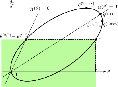
Figure 7: ${\cal D}={\cal D}^{(1)}\cap{\cal D}^{(2)}$ (left), where ${\cal D}^{(1)}$ and ${\cal D}^{(2)}$ are in Figure 5, and ${\cal D}={\cal D}^{(2)}$ (right)

Define

$$\tau_{i}=\sup\{\theta_{i}>0;\theta\in{\cal D}_{1}\cap{\cal D}_{2}\},\qquad i=1,2.$$ (3.25)

Theorem 3.2.

Assume conditions (2.1) and (2.2). Then, (a)

$${\cal D}={\cal D}^{(1)}\cap{\cal D}^{(2)}.$$ (3.26)

(b) The large deviations rate function $I$ is obtained as

$$I(v)=\left\{\begin{array}[]{ll}\min(\big{\langle}v,\tilde{\theta}^{(1,\rm r)}\big{\rangle},\big{\langle}v,\tilde{\theta}^{(2,\rm r)}\big{\rangle}),&\tau\in\Gamma,\\ \sup\{\left\langle v,\theta\right\rangle;\theta\in{\cal D}\},&\tau\not\in\Gamma,\end{array}\right.$$ (3.29)

In particular,

$$I({\rm e}^{(i)})=\tau_{i},\qquad i=1,2,$$ (3.30)

where

$${\rm e}^{(1)}=\begin{pmatrix}1\\ 0\end{pmatrix}\quad\text{ and }\quad{\rm e}^{(2)}=\begin{pmatrix}0\\ 1\end{pmatrix}.$$

Remark 3.2.

Theorems 3.1 and 3.2 provide a geometrical interpretation for Theorem 3.1 of [1]. The latter is algebraic. This interpretation does not mean that the value function $I(v)$ is analytically easier to compute. However, it enables us to see how $I(v)$ is changing with $v$ and how $I(v)$ is influenced by the primitive data through the domain ${\cal D}$ and two points $\theta^{(1,{\rm r})}$ and $\theta^{(2,{\rm r})}$.

Figure 8 gives an illustration of the rate function given in (3.29). The following corollary is immediate. Inequality (3.31) below is also proved in [5, Section 8].

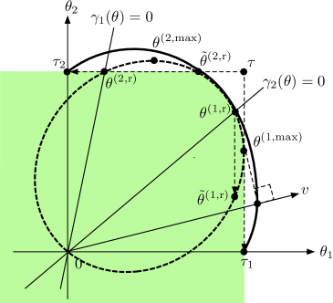
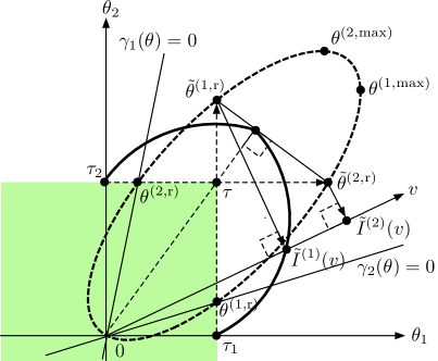
Figure 8: The shapes of the rate functions $I(v)$ with $\|v\|=1$ are drawn by thick curves; $\tau$ is inside the ellipse in the right panel and is outside in the left panel

Corollary 3.2.

For each $v\in\mathbb{R}^{2}_{+}$,

$$I(v)\geq\sup\{\left\langle v,\theta\right\rangle;\theta\in{\cal D}\}.$$ (3.31)

Proof of Theorem 3.2.

We first prove (a). Here, we adopt the following three categories, which are introduced in [5].

$$\text{Category I:\ \ }\quad\theta^{(2,\Gamma)}_{1}<\theta^{(1,\Gamma)}_{1}\mbox{ and }\theta^{(1,\Gamma)}_{2}<\theta^{(2,\Gamma)}_{2},$$ (3.32)

$$\text{Category II: }\quad\theta^{(2,\Gamma)}\leq\theta^{(1,\Gamma)},$$ (3.33)

$$\text{Category III:}\quad\theta^{(1,\Gamma)}\leq\theta^{(2,\Gamma)}.$$ (3.34)

It is immediate from the definitions of ${\cal D}^{(1)}$ and ${\cal D}^{(2)}$ that

$${\cal D}^{(1)}\cap{\cal D}^{(2)}$$

$$=\Bigl{\{}\theta\in\mathbb{R}^{2};\text{ there exists a }\theta^{\prime}\in\Gamma\text{ such that }\theta<\theta^{\prime},\theta_{1}^{\prime}<\theta^{(1,\Gamma)}_{1}\text{ and }\theta_{2}^{\prime}<\theta^{(2,\Gamma)}_{2}\Bigr{\}}.$$

Hence, $\theta\in{\cal D}^{(1)}\cap{\cal D}^{(2)}$ implies that

$$\theta<\bigl{(}\theta^{(1,\Gamma)}_{1},\theta^{(2,\Gamma)}_{2}\bigr{)}^{T}$$ (3.35)

for all categories. For Category I, (3.35) and $\theta\in\Gamma_{\max}$ implies $\theta\in{\cal D}^{(1)}\cap{\cal D}^{(2)}$. For Category II, $\theta^{(2,\Gamma)}\leq\theta^{(1,\Gamma)}$ implies that $\theta^{(2,\Gamma)}_{2}<\theta^{(2,\max)}_{2}$, and therefore $\theta^{(2,\max)}\not\in\Gamma_{2}$. Hence, ${\cal D}^{(1)}\cap{\cal D}^{(2)}$ is equal to $\{\theta\in\mathbb{R}^{2};\theta<\tilde{\theta}^{(2,\rm r)}\}$ by Lemma 3.1. Thus, we have the following expression by the symmetry of Categories II and III.

$${\cal D}^{(1)}\cap{\cal D}^{(2)}=\left\{\begin{array}[]{ll}\Bigl{\{}\theta\in\Gamma_{\max};\theta<\bigl{(}\theta^{(1,\Gamma)}_{1},\theta^{(2,\Gamma)}_{2}\bigr{)}^{T}\Bigr{\}},&\mbox{for Category I},\\ \{\theta\in\mathbb{R}^{2};\theta<\tilde{\theta}^{(2,\rm r)}\},&\mbox{for Category II},\\ \{\theta\in\mathbb{R}^{2};\theta<\tilde{\theta}^{(1,\rm r)}\},&\mbox{for Category III}.\end{array}\right.$$

This implies that

$$\tau=\left\{\begin{array}[]{ll}\bigl{(}\theta^{(1,\Gamma)}_{1},\theta^{(2,\Gamma)}_{2}\bigr{)}^{T},&\mbox{for in Category I},\\ \tilde{\theta}^{(2,\rm r)},&\mbox{for Category II},\\ \tilde{\theta}^{(1,\rm r)},&\mbox{for Category III}.\end{array}\right.$$ (3.40)

Thus, the $\tau$ is identical with the one that is obtained in [5]. Since Theorem 2.1 of [5] says that

$${\cal D}=\{\theta\in\Gamma_{\max};\theta<\tau\},$$ (3.41)

(3.26) is proved. We next prove part (b). For this, we consider the two cases, $\tau\in\Gamma$ and $\tau\not\in\Gamma$, separately. First assume that $\tau\in\Gamma$ (see, e.g., the left picture of Figure 4). In this case, ${\rm n}^{\Gamma}(\tilde{\theta}^{(1,\rm r)})$ is above ${\rm n}^{\Gamma}(\tilde{\theta}^{(2,\rm r)})$, and therefore we have the following three cases for nonzero $v\in\mathbb{R}_{+}^{2}$ by Lemma 3.2 and its symmetric version for ${\cal D}^{(2)}$. If $v$ is below ${\rm n}^{\Gamma}(\tilde{\theta}^{(2,\rm r)})$ or on ${\rm n}^{\Gamma}(\tilde{\theta}^{(2,\rm r)})$, then

$$I^{(1)}(v)=\big{\langle}v,\tilde{\theta}^{(1,\rm r)}\big{\rangle}\mbox{ and }I^{(2)}(v)=\sup\{\big{\langle}v,\theta\big{\rangle};\theta\in\Gamma\}.$$

If $v$ is between ${\rm n}^{\Gamma}(\tilde{\theta}^{(2,\rm r)})$ and ${\rm n}^{\Gamma}(\tilde{\theta}^{(1,\rm r)})$, then

$$I^{(1)}(v)=\big{\langle}v,\tilde{\theta}^{(1,\rm r)}\big{\rangle}\mbox{ and }I^{(2)}(v)=\big{\langle}v,\tilde{\theta}^{(2,\rm r)}\big{\rangle}.$$

If $v$ is above ${\rm n}^{\Gamma}(\tilde{\theta}^{(1,\rm r)})$ or on ${\rm n}^{\Gamma}(\tilde{\theta}^{(1,\rm r)})$, then

$$I^{(1)}(v)=\sup\{\big{\langle}v,\theta\big{\rangle};\theta\in\Gamma\}\mbox{ and }I^{(2)}(v)=\big{\langle}v,\tilde{\theta}^{(2,\rm r)}\big{\rangle}.$$

Thus, we have (3.29) for $\tau\in\Gamma$ because $I^{(1)}(v)\leq I^{(2)}(v)$ for the first case, and $I^{(2)}(v)\leq I^{(1)}(v)$ for the third case.

We next suppose that $\tau\not\in\Gamma$ (see, e.g., Figure 5). In this case, ${\rm n}^{\Gamma}(\tilde{\theta}^{(1,\rm r)})$ is not above ${\rm n}^{\Gamma}(\tilde{\theta}^{(2,\rm r)})$, and we similarly have the following three cases. If $v$ is below ${\rm n}^{\Gamma}(\tilde{\theta}^{(1,\rm r)})$ or on ${\rm n}^{\Gamma}(\tilde{\theta}^{(1,\rm r)})$, then

$$I^{(1)}(v)=\big{\langle}v,\tilde{\theta}^{(1,\rm r)}\big{\rangle}\mbox{ and }I^{(2)}(v)=\sup\{\big{\langle}v,\theta\big{\rangle};\theta\in\Gamma\}.$$

If $v$ is between ${\rm n}^{\Gamma}(\tilde{\theta}^{(1,\rm r)})$ and ${\rm n}^{\Gamma}(\tilde{\theta}^{(2,\rm r)})$, then

$$I^{(1)}(v)=I^{(2)}(v)=\sup\{\big{\langle}v,\theta\big{\rangle};\theta\in\Gamma\}.$$

If $v$ is above ${\rm n}^{\Gamma}(\tilde{\theta}^{(2,\rm r)})$ or on ${\rm n}^{\Gamma}(\tilde{\theta}^{(2,\rm r)})$, then

$$I^{(1)}(v)=\sup\{\big{\langle}v,\theta\big{\rangle};\theta\in\Gamma\}\mbox{ and }I^{(2)}(v)=\big{\langle}v,\tilde{\theta}^{(2,\rm r)}\big{\rangle}.$$

In the first case, $I^{(1)}(v)\leq I^{(2)}(v)$, and $I^{(1)}(v)=\sup\{\big{\langle}v,\theta\big{\rangle};\theta\in{\cal D}\}$, while in the third case $I^{(2)}(v)\leq I^{(1)}(v)$, and $I^{(2)}(v)=\sup\{\big{\langle}v,\theta\big{\rangle};\theta\in{\cal D}\}$. Hence, we always have

$$\min(I^{(1)}(v),I^{(2)}(v))=\sup\{\big{\langle}v,\theta\big{\rangle};\theta\in{\cal D}\}.$$

Thus, we obtain (3.29) for $\tau\not\in\Gamma$.

We finally prove (3.30). This is immediate from (3.29), (3.25) and (3.26) if $\tau\not\in\Gamma$. Otherwise, $I(v)=\min(\big{\langle}v,\tilde{\theta}^{(1,\rm r)}\big{\rangle},\big{\langle}v,\tilde{\theta}^{(2,\rm r)}\big{\rangle})$ by (3.29). This implies (3.30) since $\big{\langle}{\rm e}^{(1)},\tilde{\theta}^{(1,\rm r)}\big{\rangle}<\big{\langle}{\rm e}^{(1)},\tilde{\theta}^{(2,\rm r)}\big{\rangle}$ and $\big{\langle}{\rm e}^{(2)},\tilde{\theta}^{(2,\rm r)}\big{\rangle}<\big{\langle}{\rm e}^{(2)},\tilde{\theta}^{(1,\rm r)}\big{\rangle}$ for $\tau\in\Gamma$. This completes the proof. ∎

4 Characterization by Avram, Dai and Hasenbein

Theorem 6.3 of [1] gives explicit expressions for $I^{(i)}(v)$ for each $v\in\mathbb{R}^{2}_{+}$. We will use these expressions to prove Theorem 3.1. For concreteness, we will prove Theorem 3.1 for $i=1$. Recall $\theta^{(v,\Gamma)}$ defined in (3.20). The next lemma gives an analytical expression for $\langle v,\theta^{(v,\Gamma)}\rangle$.

Lemma 4.1.

For each $v\in\mathbb{R}^{2}_{+}$,

$$\left\langle v,\theta^{(v,\Gamma)}\right\rangle=\sqrt{\left\langle\mu,\Sigma^{-1}\mu\right\rangle\left\langle v,\Sigma^{-1}v\right\rangle}-\left\langle\mu,\Sigma^{-1}v\right\rangle.$$ (4.1)

Proof.

Obviously, the right side of (3.20) is attained by the $\theta$ on the ellipse $\partial\Gamma$ such that $v$ parallels the normal $n^{\Gamma}(\theta)$ at the $\theta$. That is, $v$ is proportional to ${\rm n}^{\Gamma}(\theta)$. Thus, following (3.18), we have for some $\alpha>0$,

$$\Sigma\theta+\mu=\alpha v.$$

Substituting $\theta=\Sigma^{-1}(\alpha v-\mu)$ in $\gamma(\theta)=0$, we have

$$\alpha=\sqrt{\frac{\left\langle\Sigma^{-1}\mu,\mu\right\rangle}{\left\langle\Sigma^{-1}v,v\right\rangle}}.$$

Hence,

$$\left\langle v,\theta\right\rangle=\left\langle\Sigma^{-1}(\alpha v-\mu),v\right\rangle=\sqrt{\left\langle\mu,\Sigma^{-1}\mu\right\rangle\left\langle v,\Sigma^{-1}v\right\rangle}-\left\langle\Sigma^{-1}\mu,v\right\rangle.$$

This proves (4.1). ∎

Central in the proofs of Avram et al. [1] is two vectors $a^{2}$ and $\tilde{a}^{2}$ defined in (3.2) and (3.4), respectively, of their paper. They call $\tilde{a}^{2}$ the symmetry of $a^{2}$ around face $F_{2}=\{z=(z_{1},z_{2})\in\mathbb{R}^{2}_{+};z_{2}=0\}$, namely the nonnegative horizontal axis. (Readers are warned again the swap of indexes between [1] and this paper. Anything pertaining to the horizontal axis is indexed as $1$, with a pair of parentheses, in this paper, and is indexed as $2$ in [1].)

It follows from (3.7) and (3.18) of this paper and (3.2) of [1] that one immediately has the following geometric interpretation

$$a^{2}=n^{\Gamma}(\theta^{(1,\rm r)}).$$ (4.2)

(Note that our $\theta^{(1,\rm r)}$ in (3.7) has denominator $\langle p^{(1)},\Sigma p^{(1)}\rangle$ because our $p^{(1)}$ is not normalized.) To introduce their symmetry $\tilde{a}^{2}$ using their (3.4) in [1], we introduce

$${\rm e}^{2}=\begin{pmatrix}1\\ 0\end{pmatrix}\quad\text{ and }n^{2}=\begin{pmatrix}0\\ 1\end{pmatrix}.$$ (4.3)

One can check that the vector $a^{2}$ (or any other vector) has the following orthogonal decomposition under inner product $\langle\Sigma^{-1}x,y\rangle$ for $x,y\in\mathbb{R}^{2}$.

$$a^{2}=\frac{\langle\Sigma^{-1}a^{2},{\rm e}^{2}\rangle}{\langle\Sigma^{-1}{\rm e}^{2},{\rm e}^{2}\rangle}{\rm e}^{2}+\frac{\langle a^{2},n^{2}\rangle}{\langle\Sigma n^{2},n^{2}\rangle}\Sigma n^{2}.$$ (4.4)

The dominators in (4.4) are due to the lacking of normalization in (4.3). Their (3.4) defines $\tilde{a}^{2}$ via

$$\tilde{a}^{2}=\frac{\langle\Sigma^{-1}a^{2},{\rm e}^{2}\rangle}{\langle\Sigma^{-1}{\rm e}^{2},{\rm e}^{2}\rangle}{\rm e}^{2}-\frac{\langle a^{2},n^{2}\rangle}{\langle\Sigma n^{2},n^{2}\rangle}\Sigma n^{2}.$$ (4.5)

The following equation gives the geometric interpretation of $\tilde{a}^{2}$.

$$\tilde{a}^{2}=n^{\Gamma}(\tilde{\theta}^{(1,\rm r)}).$$ (4.6)

We leave the proof of (4.6) to the end of this section.

Following Definition 3.2 and equation (3.5) of [1], the face $F_{2}$ is reflective if and only if

$$\tilde{a}^{2}_{2}>0.$$ (4.7)

The following lemma is immediate.

Lemma 4.2.

Face $F_{2}$ is reflective if and only if condition (3.10) is not satisfied.

Now we are ready to prove Theorem 3.1.

Proof of Theorem 3.1.

We prove Theorem 3.1 for $i=1$. First assume that condition (3.10) is satisfied. In this case, $\tilde{a}_{2}^{2}\leq 0$ and the face $F_{2}$ is not reflective. It follows from part (b) of Theorem 6.3 in [1], for any $v\in\mathbb{R}^{2}_{+}$, $I^{(1)}(v)$ is given by the expression (3.6) of [1], which is the right side of (4.1). Thus, in this case,

$$I^{(1)}(v)=\langle v,\theta^{(v,\Gamma)}\rangle=\sup\{\langle v,\theta\rangle;\theta\in\Gamma\}=\sup\{\langle v,\theta\rangle;\theta\in\Gamma_{\max}\},$$

which is $\sup\{\langle v,\theta\rangle;\theta\in{\cal D}^{(1)}\}$ because ${\cal D}^{(1)}=\Gamma_{\max}$.

Now assume that condition (3.10) is not satisfied. In this case, $\tilde{a}_{2}^{2}>0$ and the face $F_{2}$ is reflective. If $\tilde{\theta}^{(1,\rm r)}$ is to the left of $\theta^{(2,\max)}$, then $\tilde{a}^{2}_{1}<0$. Thus, for any $v\in\mathbb{R}^{2}_{+}$, $v$ is below $\tilde{a}^{2}$. It follows from part (a) in Theorem 6.3 of [1], for any $v\in\mathbb{R}^{2}_{+}$, $I^{(1)}(v)$ is given by

$$\langle v,\tilde{\theta}^{(1,\rm r)}\rangle,$$

which is equal to $\sup\{\langle v,\theta\rangle;\theta\in{\cal D}^{(1)}\}$ by Lemma 3.2. Otherwise, we have that $\tilde{\theta}^{(1,\rm r)}$ is to the right of or equal to $\theta^{(2,\max)}$. Thus, $\tilde{a}^{2}_{1}\geq 0$. It follows from part (b) in Theorem 6.3 of [1] for any $v\in\mathbb{R}^{2}_{+}$ that is on or above $\tilde{a}^{2}$, $I^{(1)}(v)$ is again given by the right side of (4.1), which is equal to $\langle v,\theta^{(v,\Gamma)}\rangle$, and therefore to $\sup\{\langle v,\theta\rangle;\theta\in{\cal D}^{(1)}\}$ by Lemma 3.2. When $v\in\mathbb{R}^{2}_{+}$ is below $\tilde{a}^{2}$, it follows again from part (a) in Theorem 6.3 of [1] that $I^{(1)}(v)$ is given by

$$\langle v,\tilde{\theta}^{(1,\rm r)}\rangle,$$

which is equal to $\sup\{\langle v,\theta\rangle;\theta\in{\cal D}^{(1)}\}$ by Lemma 3.2. ∎

Proof of equation (4.6).

Because $\gamma(\theta^{(1,\rm r)})=0$, we have by (4.2)

$$\left\langle\Sigma^{-1}(a^{2}-\mu),(a^{2}-\mu)\right\rangle+2\left\langle\mu,\Sigma^{-1}(a^{2}-\mu)\right\rangle=0,$$

and therefore

$$\left\langle a^{2},\Sigma^{-1}a^{2}\right\rangle=\left\langle\mu,\mu\right\rangle.$$ (4.8)

From (4.5), we have

$$\left\langle\tilde{a}^{2},\Sigma^{-1}{\rm e}^{2}\right\rangle=\left\langle\Sigma^{-1}\tilde{a}^{2},{\rm e}^{2}\right\rangle=\frac{\left\langle\Sigma^{-1}a^{2},{\rm e}^{2}\right\rangle}{\left\langle\Sigma^{-1}{\rm e}^{2},{\rm e}^{2}\right\rangle}\left\langle\Sigma^{-1}{\rm e}^{2},{\rm e}^{2}\right\rangle=\left\langle\Sigma^{-1}a^{2},{\rm e}^{2}\right\rangle.$$ (4.9)

Hence,

$$\left\langle\tilde{a}^{2},\Sigma^{-1}\tilde{a}^{2}\right\rangle = \frac{\left\langle\Sigma^{-1}a^{2},{\rm e}^{2}\right\rangle\left\langle\tilde{a}^{2},\Sigma^{-1}{\rm e}^{2}\right\rangle}{\left\langle\Sigma^{-1}{\rm e}^{2},{\rm e}^{2}\right\rangle}-\frac{\left\langle a^{2},{n}^{2}\right\rangle\left\langle\tilde{a}^{2},{n}^{2}\right\rangle}{\left\langle\Sigma n^{2},n^{2}\right\rangle}$$

$$= \frac{\left\langle\Sigma^{-1}a^{2},{\rm e}^{2}\right\rangle^{2}}{\left\langle\Sigma^{-1}{\rm e}^{2},{\rm e}^{2}\right\rangle}+\frac{\left\langle a^{2},{n}^{2}\right\rangle^{2}}{\left\langle\Sigma n^{2},n^{2}\right\rangle}$$

$$= \left\langle a^{2},\Sigma^{-1}a^{2}\right\rangle.$$

This and (4.8) imply

$$\left\langle\tilde{a}^{2},\Sigma^{-1}\tilde{a}^{2}\right\rangle=\left\langle\mu,\mu\right\rangle,$$

which is equivalent to $\gamma(\Sigma^{-1}(\tilde{a}^{2}-\mu))=0$. Thus, the point

$$\Sigma^{-1}(\tilde{a}^{2}-\mu)$$

is on the ellipse. From equations (4.4) and (4.5), the first component of

$$\Sigma^{-1}(\tilde{a}^{2}-\mu)$$

is equal to the first component of $\Sigma^{-1}({a}^{2}-\mu)$, which is $\theta^{(1,\rm r)}_{1}$. Also, from (4.4) and (4.5), $\tilde{a}^{2}=a^{2}$ if and only if $\langle a^{2},n^{2}\rangle=0$. The latter is equivalent to the normal direction $a^{2}$ at $\theta^{(1,\rm r)}$ being horizontal or $\theta^{(1,\rm r)}=\theta^{(1,\max)}$. Thus, we have either $\Sigma^{-1}(\tilde{a}^{2}-\mu)\neq\theta^{(1,\rm r)}$ or $\Sigma^{-1}(\tilde{a}^{2}-\mu)=\theta^{(1,\rm r)}=\theta^{(1,\max)}$. Therefore, we have proved that

$$\Sigma^{-1}(\tilde{a}^{2}-\mu)=\tilde{\theta}^{(1,\rm r)},$$

which is equivalent to (4.6). ∎

5 Product form stationary distribution

Harrison and Williams [10] proved that a multi-dimensional SRBM has a product form stationary distribution if and only if the SRBM data $(\Sigma,\mu,R)$ satisfies $R^{-1}\mu<0$ and the skew symmetry condition

$$2\Sigma=R\Delta_{R}^{-1}\Delta_{\Sigma}+\Delta_{\Sigma}\Delta_{R}^{-1}R^{{\mbox{\scriptsize\sc t}}}$$ (5.1)

is satisfied, where, for a matrix $A$, $\Delta_{A}$ is the diagonal matrix whose diagonal entries are that of $A$. In this section, we prove the following theorem.

Theorem 5.1.

Assume that (2.1) and (2.2) hold. The two-dimensional SRBM has a product form stationary distribution if and only if

$$\tilde{\theta}^{(1,\rm r)}=\tilde{\theta}^{(2,\rm r)},$$ (5.2)

holds, where $\tilde{\theta}^{(i,r)}$ is the symmetry of $\theta^{(i,r)}$ defined in (3.9).

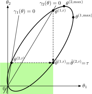
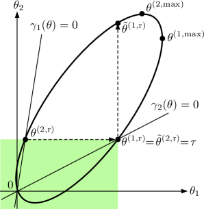
Figure 9: The locations $\theta^{(1,\rm r)}$ and $\theta^{(2,\rm r)}$; left panel is for product form; the right panel is for non-product form

Figure 9 gives examples for the locations of $\tilde{\theta}^{(1,\rm r)}$ and $\tilde{\theta}^{(2,\rm r)}$; left panel illustrates an SRBM whose data satisfies (5.2), and the right panel illustrates an SRBM whose data does not satisfy (5.2). Equation (5.2) provides a geometric condition on the SRBM data for the stationary distribution to have a product form. Of course, the algebraic condition (5.1) and geometric condition (5.2) must be equivalent although its verification is not obvious.

Remark 5.1.

Avram et al. [1] proved that the skew symmetry condition (5.1) implies

$$\tilde{a}^{1}=\tilde{a}^{2},$$ (5.3)

where $\tilde{a}^{2}$ is defined in (4.5) and $\tilde{a}^{1}$ is defined similarly. Because $\tilde{a}^{2}=n^{\Gamma}(\tilde{\theta}^{(1,\rm r)})$ and $\tilde{a}^{1}=n^{\Gamma}(\tilde{\theta}^{(2,\rm r)})$, where $n^{\Gamma}(\theta)$ is the outward normal of the ellipse at $\theta$, condition (5.3) is equivalent to condition (5.2). Thus, geometric condition (5.2) is necessary for the stationary distribution to have a product form.

We will provide a complete proof of Theorem 5.1 at the end of this section. Before that, we provide some background discussion on the product form stationary distribution. It is known that the stationary distribution has a density; see, for example, [9] and [3]. We use $\zeta(x,y)$ to denote the stationary density of the two-dimensional SRBM. Thus, the stationary distribution has a product form if and only if

$$\zeta(x,y)=\zeta_{1}(x)\zeta_{2}(y)\quad\text{ for }x,y\in\mathbb{R}_{+},$$ (5.4)

where $\zeta_{i}$’s are the marginal densities of $\zeta$. It follows from [10] that when the stationary density is of the product form in (5.4), each marginal density $\zeta_{i}$ must be exponential. Hence, the product form holds if and only if there exist some $\alpha_{1},\alpha_{2}>0$ such that

$$\zeta(x,y)=\alpha_{1}\alpha_{2}e^{-(\alpha_{1}x+\alpha_{2}y)}\quad\text{ for }x,y\geq 0.$$ (5.5)

Harrison and Williams [10] proved that when the stationary density is of the product form, $\alpha$ is given by

$$\alpha=-2\Delta_{\Sigma}^{-1}\Delta_{R}R^{-1}\mu.$$ (5.6)

Associated with the stationary distribution are two boundary measures $\nu_{1}$ and $\nu_{2}$. The measure $\nu_{i}$ has support on $F_{i}=\{z\in\mathbb{R}^{2}_{+};z_{i}=0\}$, $i=1,2$; see, for example, Section 2 of [5] for their definition. It is known that the stationary distribution, together with its associated boundary measures, satisfies the basic adjoint relationship (BAR). For a statement of BAR in two dimensions, see, for example, (4.1) of [5]. Harrison and Williams [9] proved the necessity of BAR when the reflection matrix $R$ is an ${\cal M}$ matrix and the stability condition $R^{-1}\mu<0$ is satisfied. Assuming the stationary distribution exists, Dai and Harrison [3] proved the necessity of BAR for a general reflection matrix $R$ that is completely-${\cal S}$.

Recall the two-dimensional moment generating function $\varphi(\theta)$ defined in (3.1) for the stationary distribution. We denote the moment generating functions of boundary measures $\nu_{1}$ and $\nu_{2}$ by $\varphi_{1}(\theta_{2})$ and $\varphi_{2}(\theta_{1})$, respectively. Then, Dai and Miyazawa [5] derived from the basic adjoint relationship the following key relationship among moment generating functions:

$$\gamma(\theta)\varphi(\theta)=\gamma_{1}(\theta)\varphi_{1}(\theta_{2})+\gamma_{2}(\theta)\varphi_{2}(\theta_{1})$$ (5.7)

for any $\theta\in\mathbb{R}^{2}$ as long as $\varphi(\theta)$ is finite.

Proof of Theorem 5.1.

Remark 5.1 proves the necessity of the theorem. Here, we provide a self-contained, alternative proof for the necessity. The technique used in our necessity proof will be useful in the sufficiency proof.

Assume that the stationary distribution has the product form stationary density given by (5.5). It follows from [9] that boundary measure $\nu_{1}$ has density

$$\zeta_{1}(y)=\frac{\Sigma_{11}}{2r_{11}}\zeta(0,y)=\frac{\Sigma_{11}}{2r_{11}}\alpha_{1}\alpha_{2}e^{-\alpha_{2}y}\quad\text{ for }y\geq 0$$ (5.8)

such that

$$\nu_{1}(\mathbb{R}_{+}\times B)=\int_{B}\zeta_{1}(y)dy\quad\text{ for any Borel set $B$ in $\mathbb{R}_{+}$}.$$ (5.9)

Similarly, boundary measure $\nu_{2}$ has density

$$\zeta_{2}(x)=\frac{\Sigma_{22}}{2r_{22}}\zeta(x,0)=\frac{\Sigma_{22}}{2r_{22}}\alpha_{1}\alpha_{2}e^{-\alpha_{2}x}\quad\text{ for }x\geq 0$$ (5.10)

such that

$$\nu_{2}(A\times\mathbb{R}_{+})=\int_{A}\zeta_{2}(y)dy\quad\text{ for any Borel set $A$ in $\mathbb{R}_{+}$}.$$ (5.11)

It follows from (5.5), (5.8) and (5.10) that

$$\varphi(\theta)=\frac{\alpha_{1}}{\alpha_{1}-\theta_{1}}\frac{\alpha_{2}}{\alpha_{2}-\theta_{2}}\quad\text{ for $\theta\in\mathbb{R}^{2}$ with }\theta<\alpha,$$ (5.12)

$$\varphi_{1}(\theta_{2})=\frac{\Sigma_{11}\alpha_{1}\alpha_{2}}{2r_{11}(\alpha_{2}-\theta_{2})}\quad\text{ for }\theta_{2}<\alpha_{2},$$ (5.13)

$$\varphi_{2}(\theta_{1})=\frac{\Sigma_{22}\alpha_{1}\alpha_{2}}{2r_{22}(\alpha_{1}-\theta_{1})}\quad\text{ for }\theta_{1}<\alpha_{1}.$$ (5.14)

Plugging these expressions for $\varphi(\theta)$, $\varphi_{1}(\theta_{2})$, and $\varphi_{2}(\theta_{1})$ into key relationship (5.7), we have

$$\gamma(\theta)=\frac{\Sigma_{22}}{2r_{22}}\gamma_{2}(\theta)(\alpha_{2}-\theta_{2})+\frac{\Sigma_{11}}{2r_{11}}\gamma_{1}(\theta)(\alpha_{1}-\theta_{1})\quad\text{ for any }\theta<\alpha.$$ (5.15)

Note that both sides of (5.15) are quadratic functions of $\theta$. Since (5.15) holds for any $\theta<\alpha$ and a quadratic function of two variables is uniquely determined by six points, it must hold for all $\theta\in\mathbb{R}^{2}$. In particular, we have

$$\gamma(\alpha)=0$$ (5.16)

That is, $\alpha$ must be on the ellipse $\partial\Gamma$. Plugging $\theta=\theta^{(1,\rm r)}$ into (5.15) implies that

$$\alpha_{1}=\theta^{(1,\rm r)}_{1}=\tilde{\theta}^{(1,\rm r)}_{1}$$ (5.17)

because $\gamma(\theta^{(1,\rm r)})=0$, $\gamma_{2}(\theta^{(1,r)})=0$ and $\gamma_{1}(\theta^{(1,\rm r)})\neq 0$; see Lemma 2.2 of [5] for the latter. Plugging $\theta=\tilde{\theta}^{(1,\rm r)}$ into (5.15), we have

$$\frac{\Sigma_{22}}{2r_{22}}\gamma_{2}(\tilde{\theta}^{(1,\rm r)})(\alpha_{2}-\tilde{\theta}^{(1,\rm r)}_{2})=0$$ (5.18)

because $\gamma(\tilde{\theta}^{(1,\rm r)})=0$ and $\alpha_{1}=\tilde{\theta}^{(1,\rm r)}_{1}$. If $\tilde{\theta}^{(1,\rm r)}=\theta^{(1,\rm r)}$, then $\theta^{(1,\rm r)}=\theta^{(1,\max)}$. This fact, together with (5.16) and (5.17), implies that

$$\alpha_{2}=\tilde{\theta}^{(1,\rm r)}_{2}.$$ (5.19)

If $\tilde{\theta}^{(1,\rm r)}\neq\theta^{(1,\rm r)}$, then $\gamma_{2}(\tilde{\theta}^{(1,\rm r)})\neq 0$, and (5.18) implies again (5.19). Equations (5.17) and (5.19) imply that

$$\alpha=\tilde{\theta}^{(1,\rm r)}.$$ (5.20)

Similarly, we can prove

$$\alpha=\tilde{\theta}^{(2,\rm r)}.$$ (5.21)

Equations (5.20) and (5.21) imply that (5.2) holds, proving the necessity of the theorem.

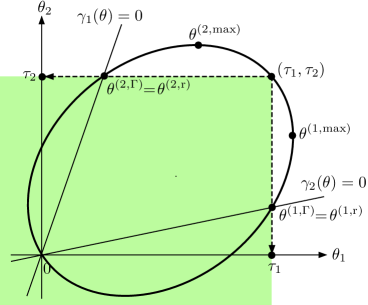
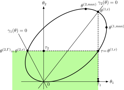
Figure 10: The locations of $\tau$, $\theta^{(1,\rm r)}$ and $\theta^{(2,\rm r)}$ for the product form

We now prove the sufficiency of the theorem. Assume (5.2) holds. Let

$$\alpha=\tilde{\theta}^{(1,\rm r)}=\tilde{\theta}^{(2,\rm r)}.$$

Then, $\alpha$ is on the ellipse, and thus $\gamma(\alpha)=0$. Therefore,

$$\gamma(\theta) = \gamma(\theta)-\gamma(\alpha)=\frac{1}{2}\Bigl{[}\langle\alpha,\Sigma\alpha\rangle-\langle\theta,\Sigma\theta\rangle\Bigr{]}+\langle\mu,\alpha\rangle-\langle\mu,\theta\rangle$$ (5.22)

$$= \Bigl{\langle}\alpha-\theta,\frac{1}{2}\Sigma(\theta+\alpha)+\mu\Bigr{\rangle}$$

$$= f_{1}(\theta)(\alpha_{1}-\theta_{1})+f_{2}(\theta)(\alpha_{2}-\theta_{2}),$$

where

$$\begin{pmatrix}f_{1}(\theta)\\ f_{2}(\theta)\end{pmatrix}=\frac{1}{2}\Sigma(\theta+\alpha)+\mu.$$

Also, $\gamma(0)=0$ gives

$$\alpha_{1}f_{1}(0)+\alpha_{2}f_{2}(0)=0.$$

Therefore, there exists a $k\in\mathbb{R}$ such that

$$\begin{pmatrix}f_{1}(0)\\ f_{2}(0)\end{pmatrix}=k\begin{pmatrix}\alpha_{2}\\ -\alpha_{1}\end{pmatrix}.$$ (5.23)

It follows from (5.22) that

$$\gamma(\theta) = \Bigl{(}f_{1}(\theta)-k(\alpha_{2}-\theta_{2})\Bigr{)}(\alpha_{1}-\theta_{1})+\Bigl{(}f_{2}(\theta)+k(\alpha_{1}-\theta_{1})\Bigr{)}(\alpha_{2}-\theta_{2})$$ (5.24)

$$= \tilde{f}_{1}(\theta)(\alpha_{1}-\theta_{1})+\tilde{f}_{2}(\theta)(\alpha_{2}-\theta_{2}),$$

where

$$\tilde{f}_{1}(\theta)=f_{1}(\theta)-k(\alpha_{2}-\theta_{2}),$$

$$\tilde{f}_{2}(\theta)=f_{2}(\theta)+k(\alpha_{1}-\theta_{1}).$$

Both functions $\tilde{f}_{1}(\theta)$ and $\tilde{f}_{2}(\theta)$ are linear in $\theta$ and (5.23) implies that $\tilde{f}_{1}(0)=0$ and $\tilde{f}_{2}(0)=0$. If $\alpha\neq\theta^{(1,\rm r)}$, substituting $\theta=\theta^{(1,\rm r)}$ into equation (5.24) yields

$$\tilde{f}_{2}(\theta^{(1,\rm r)})=0.$$ (5.25)

If $\alpha=\theta^{(1,\rm r)}$, we have $\theta^{(1,\rm r)}=\theta^{(1,\max)}$,

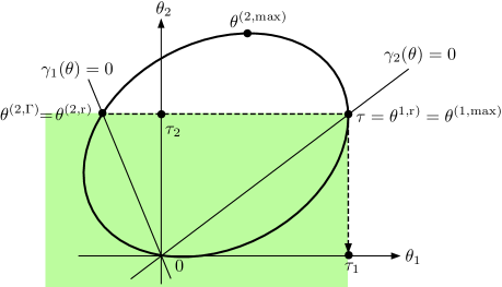
Figure 11: The case that $\theta^{(1,\rm r)}=\theta^{(1,\max)}$ for the product form

which implies

$$\left.\frac{\partial}{\partial\theta_{2}}\gamma(\theta)\right|_{\theta=\theta^{(1,\rm r)}}=0,$$

from which (5.25) follows again. Thus, we have proved that two linear equations, $\tilde{f}_{2}(\theta)=0$ and $\gamma_{2}(\theta)=0$, both have $0$ and $\theta^{(1,\rm r)}$ as their roots. Hence, $\tilde{f}_{2}(\theta)$ must be proportional to $\gamma_{2}(\theta)$. Namely, there exists a constant $c_{2}$ such that

$$\tilde{f}_{2}(\theta)=c_{2}\gamma_{2}(\theta)\quad\text{ for all }\theta\in\mathbb{R}^{2}.$$ (5.26)

Similarly, there exists a constant $c_{1}$ such that

$$\tilde{f}_{1}(\theta)=c_{1}\gamma_{1}(\theta)\quad\text{ for all }\theta\in\mathbb{R}^{2}.$$ (5.27)

It follows from (5.24), (5.26), and (5.27) that that $\gamma(\theta)$ can be written as

$$\gamma(\theta)=c_{1}\gamma_{1}(\theta)(\alpha_{1}-\theta_{1})+c_{2}\gamma_{2}(\theta)(\alpha_{2}-\theta_{2})\quad\text{ for all }\theta\in\mathbb{R}^{2}.$$ (5.28)

Comparing the coefficients of quadratic terms in (5.28), we find

$$c_{i}=\frac{\Sigma_{ii}}{2r_{ii}},\qquad i=1,2.$$

Hence, if we define $g(\theta)$, $g_{1}(\theta_{2})$ and $g_{2}(\theta_{1})$ as

$$g(\theta)=\frac{\alpha_{1}}{\alpha_{1}-\theta_{1}}\frac{\alpha_{2}}{\alpha_{2}-\theta_{2}},\qquad g_{2}(\theta_{2})=\frac{c_{1}\alpha_{1}\alpha_{2}}{\alpha_{2}-\theta_{2}},\qquad g_{1}(\theta_{1})=\frac{c_{2}\alpha_{1}\alpha_{2}}{\alpha_{1}-\theta_{1}}\quad\text{ for }\theta<\alpha,$$

then $g,g_{1},g_{2}$ are the solutions $\varphi,\varphi_{1},\varphi_{2}$ to the key relationship (5.7). Let $\pi$ be the probability measure on $\mathbb{R}^{2}_{+}$ with $\zeta(x,y)$ in (5.5) as its density function, and $\nu_{1}$ and $\nu_{2}$ be two boundary measures defined in (5.9) and (5.11). Thus, we have proved that $\pi$, $\nu_{1}$ and $\nu_{2}$ satisfy BAR (4.1) of [5] for all exponential functions

$$f(x,y)=e^{\theta_{1}x+\theta_{2}y}\quad x,y\geq 0$$

with $\theta<\alpha$. From this, one can argue that BAR is satisfied for all $f\in C^{2}_{b}(\mathbb{R}^{2})$, the set of functions which together with their first and second order partial derivatives are continuous and bounded. It follows from [4] that BAR uniquely determines the stationary distribution. Thus, the SRBM must have $\zeta(x,y)$ in (5.5) as its stationary density. ∎

6 Exact asymptotics for boundary measures

As before, we assume the SRBM satisfies conditions (2.1) and (2.2) so that it has a unique stationary distribution. In Section 5, immediately below (5.6), we introduced two boundary measures $\nu_{1}$ and $\nu_{2}$ associated with the stationary distribution of the SRBM. In this section, we study the exact asymptotics for the tail distribution of $\nu_{i}$.

The main result of this section is Theorem 6.1, which will be stated shortly. We emphasize that Lemmas 6.1, 6.2 and 6.3 that are used in the proof of Theorem 6.1 constitute a significant contribution of this paper as well. These lemmas can potentially be used for other related problems when conditions in asymptotic inversion lemmas such as Lemmas B.1 and B.2 are difficult to check.

For convenience, we write $f_{1}(x)\sim f_{2}(x)$ as $x\to\infty$ for two functions $f_{1},f_{2}$ on $[0,\infty)$ if

$$\lim_{x\to\infty}f_{1}(x)/f_{2}(x)=1.$$

Recall $\tau$ defined in (3.25) and the three categories defined through (3.32)-(3.34) in the proof of Theorem 3.2.

Theorem 6.1.

Under conditions (2.1) and (2.2), we have the exact asymptotic:

$$\lim_{x\to\infty}\frac{\nu_{2}((x,\infty))}{x^{\kappa}e^{-\tau_{1}x}}=b>0,$$ (6.1)

for some constant $b>0$, where $\kappa$ is given below.

(a) If $\tau_{1}<\theta^{(1,\max)}_{1}$, then for Category I and Category III, $\kappa=0$, and for Category II,

$$\kappa=\left\{\begin{array}[]{ll}0,&\tau_{1}\neq\theta^{(1,\rm r)}_{1},\\ 1,&\tau_{1}=\theta^{(1,\rm r)}_{1}.\end{array}\right.$$ (6.4)

(b) If $\tau_{1}=\theta^{(1,\max)}_{1}$, then for Category I,

$$\kappa=\left\{\begin{array}[]{ll}-\frac{1}{2},&\theta^{(1,\rm r)}=\theta^{(1,\max)},\\ -\frac{3}{2},&\theta^{(1,\rm r)}\neq\theta^{(1,\max)},\end{array}\right.$$ (6.7)

and for Category II,

$$\kappa=\left\{\begin{array}[]{ll}0,&\theta^{(1,\rm r)}=\theta^{(1,\max)},\\ -\frac{1}{2},&\theta^{(1,\rm r)}\neq\theta^{(1,\max)}.\end{array}\right.$$ (6.10)

We note that, in Category III, one must have $\tau_{1}<\theta^{(1,\max)}_{1}$. Thus, we do not need to consider Category III when $\tau_{1}=\theta^{(1,\max)}_{1}$. In Section 5, we introduced the moment generating functions $\varphi_{1}(\theta_{2})$ and $\varphi_{2}(\theta_{1})$ for boundary measures $\nu_{1}$ and $\nu_{2}$. Dai and Miyazawa [5] studied analytic behaviors of $\varphi_{1}(z)$ and $\varphi_{2}(z)$ as functions of complex variable $z$. In particular, they proved that $\varphi_{2}(z)$ is analytic if $\Re{z}<\tau_{1}$ and is singular at $z=\tau_{1}$. Furthermore, they characterized the nature of the singularities at $z=\tau_{1}$. See Lemmas 6.6, 6.7 and 6.8 of [5]. We will use the singularity of $\varphi_{2}(z)$ at $\tau_{1}$ to prove Theorem 6.1. Before proving the theorem, we first introduce a series of three lemmas.

For a nonnegative function $f:\mathbb{R}_{+}\to\mathbb{R}_{+}$ that is integrable on $\mathbb{R}_{+}$, let

$$g(z)=\int_{0}^{\infty}e^{zx}f(x)dx$$ (6.11)

be its moment generating function. Assume that $g$ is analytic for $\Re z<\alpha$ and is singular at $z=\alpha$ for some $\alpha>0$. Assuming $f$ is continuous, one can apply the complex inversion formula to represent $f$ as a contour integral of $g$. From this integral representation, one then uses the singular behavior of $g$ at $z=\alpha$ to obtain the exact tail asymptotic of $f$. Doetsch [6] is a good reference for the complex inversion formula. Dai and Miyazawa [5] have successfully applied this technique to study the exact asymptotic for tail distribution of $\langle c,Z(\infty)\rangle$ in an arbitrarily given direction $c\in\mathbb{R}_{+}^{2}$. In particular, they developed two asymptotic inversion lemmas, Lemmas C.1 and C.2 of [5], that allow one to directly infer the form of exact tail asymptotics of $f$ from the singular behavior of $g$ at $z=\alpha$. With these two lemmas, there is no need to get into contour integral and complex inversion formula. For convenience, these two lemmas are reproduced in the appendix of this paper.

In order to apply one of their asymptotic inversion lemmas, one needs to verify a certain set of conditions on the moment generating function $g$. For example, to apply Lemma B.1, one often needs to verify the sufficient condition (B.2). Namely, there are some positive constants $\beta$, $a$, $b$ and $\delta$ such that

$$|g(z)|<\frac{a}{|z|^{1+\delta}}\text{ for }\Re z\in[0,\beta]\text{ and }|\Im z|>b.$$ (6.12)

In the proof of our Theorem 6.1,

$$f(x)=\nu_{2}(x,\infty)\quad\text{ for }x\geq 0$$

and the corresponding moment generating function is

$$g(z)=\frac{1}{z}(\varphi_{2}(z)-\varphi_{2}(0))\quad\Re z<\tau_{1}.$$ (6.13)

When $\tau_{1}<\theta^{(1,\max)}_{1}$, one can prove that $\varphi_{2}(z)$ is bounded in a region given by $\Re z\in[0,\tau_{1}+\epsilon]$ and $|\Im z|>b$ for some $\epsilon>0$ and some $b>0$. Still we are unable to prove condition (6.12) for some positive $\delta$. Furthermore, we do not know how to check conditions (B1a)-(B1c) of Lemma B.1 directly.

To overcome the preceding difficulty, we introduce a new technique. We develop a series of three lemmas. These lemmas may have independent interest. Let

$$T(f)(x)=\int_{x}^{\infty}f(u)du,\qquad x>0,$$

be the tail distribution of $f$. Inductively, for $n\geq 1$, define

$$T^{n}(f)(x)=\int_{x}^{\infty}T^{(n-1)}(f)(u)du,\qquad x>0,$$

where $T^{0}(f)=f$. Denote the moment generating function of $T^{n}(f)$ by $\hat{T^{n}}(f)$. Then, it is easy to see that

$$\hat{T}(f)(z)=z^{-1}\bigl{(}g(z)-g(0)\bigr{)},$$ (6.14)

$$\hat{T^{2}}(f)(z)=z^{-2}\bigl{(}g(z)-g(0)-g^{\prime}(0)z\bigr{)},$$ (6.15)

where $g=\hat{T^{0}}(f)$ is the moment generating function of $f$ given in (6.11). Thus, it is easier to get asymptotics for $T^{n}(f)$ with $n\geq 1$ because it is easier for $\hat{T^{n}}(f)(z)$ to satisfy sufficient conditions such as (6.12). Thus, if $T^{n}(f)$ have the same asymptotics as $f$, it will be more convenient to work with ${T^{n}}(f)(z)$. We will show that $f$ and $T^{n}(f)$ indeed have the same asymptotics if the asymptotic is limited to a certain exponential type.

We call a function $f$ to be ultimately nonincreasing if there is an $x_{0}$ such that $f(x)$ is nonincreasing for $x\geq x_{0}$. We have the following lemma showing the equivalence of tail asymptotics. The lemma is a converse of Lemma D.5 of [5].

Lemma 6.1.

Assume that the nonnegative function $f$ is ultimately nonincreasing. For each integer $n\geq 1$, if

• $T^{n}(f)(x)\sim b\,x^{\kappa}e^{-\alpha x}$ as $x\to\infty$ for some real number $\kappa$, positive number $b$ and nonnegative number $\alpha$,

then $f(x)\sim\alpha^{n}b\,x^{\kappa}e^{-\alpha x}$ as $x\to\infty$. In particular, (6.1a) implies that $T(f)(x)\sim\alpha^{n-1}b\,x^{\kappa}e^{-\alpha x}$ as $x\to\infty$ for any nonnegative and integrable function $f$ on $[0,\infty)$.

We defer the proof of this lemma to Appendix A. We combine this lemma with the classical asymptotic inversion results in Appendix B. The idea is very simple. We just use the moment generating function $\hat{T}(f)$ of (6.14) or $\hat{T}^{2}(f)$ of (6.15) instead of the moment generating function $g$. For this, $g$ of (6.13) is redefined in the following lemma.

Lemma 6.2.

Let

$$g(z)=\int_{0}^{\infty}e^{zx}\nu(dx)$$ (6.16)

be the moment generating function of a finite measure on $[0,\infty)$. Assume that $g$ satisfies the following two conditions

• there is a complex variable function

  $$g_{0}(z)=\frac{b}{(\alpha-z)^{k}},$$

  for some positive integers $k$, some complex number $b$ and positive numbers $\alpha,\beta$ satisfying $0<\alpha<\beta$ such that $g(z)-g_{0}(z)$ is analytic for $\Re z<\beta$,

• there exists an $\epsilon_{0}>0$ such that $g(z)-g_{0}(z)$ is bounded for all $z\in\mathbb{C}$ such that $0\leq\Re z\leq\beta$ and $|z-\alpha|>\epsilon_{0}$.

Then, we have the following exact tail asymptotic for $\nu$.

$$\nu(x,\infty)\sim\frac{b\alpha^{-1}}{\Gamma(k)}x^{k-1}e^{-\alpha x}\quad\text{ as }x\to\infty,$$ (6.17)

where, $\Gamma(\lambda)$ is the gamma function as defined in Section 53 of Volume II of [14] (see also Theorem 10.14 in its Section 54 for its integral representation), and by convention $\frac{1}{\Gamma(\lambda)}=0$ when $\lambda=0,-1,-2,\ldots$.

The asymptotic of this lemma is less sharp than that of Lemma B.1 because the lower order term in Lemma B.1 has a precise exponential form. However, we do not require for $\nu(x,\infty)$ to be continuous in $x$. Before proving this lemma, we present similarly a version of Lemma B.2. In this case, the asymptotic results are the same, but we need to restrict $\lambda$ to be greater than $-1$.

Lemma 6.3.

Assume $\nu$ and $g$ as in Lemma 6.2. Assume that there are some $\alpha>0$ and some $\delta\in[0,\frac{\pi}{2})$ such that the following two conditions hold for $g$

• $g(z)$ is analytic on on ${\cal G}_{\delta}(\alpha)\equiv\{z\in\mathbb{C};z\neq\alpha,|\arg(z-\alpha)|>\delta\}$ and is bounded on ${\cal G}_{\delta}(\alpha)\cap\{z\in\mathbb{C};|z-\alpha|>\epsilon_{0}\}$ for some $\epsilon_{0}>0$, where for $z\in\mathbb{C}\setminus\{0\}$, $\arg(z)\in(-\pi,\pi)$ is the angle of $z$;

• for some complex numbers $a,b$ and some real number $\lambda$ satisfying $\lambda\neq 0$ and $\lambda>-1$,

  $$\lim_{z\to\alpha\atop z\in{\cal G}_{\delta}(\alpha)}(\alpha-z)^{\lambda}\bigl{(}g(z)-a\bigr{)}=b.$$ (6.18)

Then

$$\nu(x,\infty)\sim\frac{b\alpha^{-1}}{\Gamma(\lambda)}x^{\lambda-1}e^{-\alpha x},\quad\text{ as }x\to\infty.$$ (6.19)

In the reminder of this section, we first prove Theorem 6.1 using Lemmas 6.1, 6.2 and 6.3. We then prove the latter two lemmas, leaving the proof of Lemma 6.1 to Appendix A.

The proof of Theorem 6.1 We will use Lemmas 6.2 and 6.3 to prove the theorem. Recall that $\varphi_{2}(z)$ is the moment generating function of boundary measure $\nu_{2}$ and it will play the role of $g(z)$ in these two lemmas.

(a) For Categories I and III, we have $\tau_{1}=\theta^{(1,\rm r)}_{1}<\theta^{(1,\max)}_{1}$. By parts (a) and (c) of Lemma 6.6 of [5], all conditions of Lemma 6.2 with $k=1$ are satisfied, and hence the lemma implies the theorem with $\kappa=0$ for this case. For Category II, if $\tau_{1}\neq\theta^{(1,\rm r)}_{1}$, then $\varphi_{2}(z)$ has a simple pole at $z=\tau_{1}$, and all the conditions of Lemma 6.2 with $k=1$ are satisfied by parts (b) and (c) of Lemma 6.6 of [5]. Otherwise, $\varphi_{2}(z)$ has a double pole at $z=\tau_{1}$, all the conditions of Lemma 6.2 with $k=2$ are similarly satisfied. In either case, Lemma 6.2 implies the theorem with $\kappa$ being given in (6.4).

(b) We apply Lemma 6.8 of [5] because $\tau_{1}=\theta^{(1,\max)}_{1}$ in this case. We use parts (c) and (d) of this lemma for Category I and II, respectively. For Category I, it is not hard to see that all the conditions of Lemma 6.3 are satisfied with $\lambda=\frac{1}{2}$ for $\theta^{(1,\rm r)}_{1}=\theta^{(1,\max)}_{1}$ and $\lambda=-\frac{1}{2}$ for $\theta^{(1,\rm r)}_{1}\not=\theta^{(1,\max)}_{1}$. Therefore the theorem is proved in this case with $\kappa$ being given in (6.7). Similarly, for Category II, all conditions of Lemma 6.3 are satisfied with $\lambda=1$ for $\theta^{(1,\rm r)}_{1}=\theta^{(1,\max)}_{1}$ and $\lambda=\frac{1}{2}$ for $\theta^{(1,\rm r)}_{1}\not=\theta^{(1,\max)}_{1}$. Thus, the lemma implies the theorem with $\kappa$ being given by (6.10).

The proof of Lemma 6.2 Let

$$f(x)=\nu(x,\infty)\quad\text{ for }x\geq 0.$$ (6.20)

We apply Lemma B.1 to $T(f)$. Let

$$f_{0}(x)=\frac{b}{\Gamma(k)}x^{k-1}e^{-\alpha x}\qquad x\geq 0,$$

$$g_{0}(z)=\frac{b}{(\alpha-z)^{k}},\qquad z\in\mathbb{C}\setminus\{\alpha\}.$$

It is clear that the moment generating function of $f_{0}$ is $g_{0}$. Since $g_{0}(0)=b\alpha^{-k}$, we have, from (6.14),

$$\hat{T}(f_{0})(z)=z^{-1}\left(g_{0}(z)-g_{0}(0)\right)=\frac{b}{\alpha^{k+1}}\sum_{\ell=1}^{k}\frac{\alpha^{\ell}}{(\alpha-z)^{\ell}}$$

This and $g_{0}^{\prime}(0)=kb\alpha^{-(k+1)}$ yield

$$\hat{T^{2}}(f_{0})(z) = z^{-2}\left(g_{0}(z)-g_{0}(0)-zg^{\prime}(0)\right)$$

$$= z^{-1}\left(\hat{T}(f_{0})-g^{\prime}(0)\right)$$

$$= z^{-1}\frac{b}{\alpha^{k+1}}\sum_{\ell=1}^{k}\left(\frac{\alpha^{\ell}}{(\alpha-z)^{\ell}}-1\right)$$

$$= \frac{b}{\alpha^{k+2}}\sum_{\ell=1}^{k}\sum_{m=1}^{\ell}\frac{\alpha^{m}}{(\alpha-z)^{m}}$$

$$= \frac{b}{\alpha^{k+2}}\sum_{m=1}^{k}(k+1-m)\frac{\alpha^{m}}{(\alpha-z)^{m}}$$

$$= \frac{b}{\alpha^{2}}\frac{1}{(\alpha-z)^{k}}+\frac{b}{\alpha^{k+2}}\sum_{m=1}^{k-1}(k+1-m)\frac{\alpha^{m}}{(\alpha-z)^{m}}.$$

We check (B1a), (B1b) and (B1c) of Lemma B.1 for $\hat{T}(f)$ and $\hat{T^{2}}(f_{0})$. Note that the continuity of $f$ of Lemma B.1 is satisfied because $T(f)(x)$ is continuous in $x$ for $f$ of (6.20). (When Lemma B.1 is applied, $\hat{T}(f)$ and $\hat{T^{2}}(f_{0})$ serve the roles of $g$ and $g_{0}$, respectively, in that lemma.) It is clear that

$$\hat{T}^{2}(f)(z)-\hat{T^{2}}(f_{0})(z)=z^{-2}\left(g(z)-g_{0}(z)-(g(0)-g_{0}(0))-z(g^{\prime}(0)-g_{0}^{\prime}(0))\right)$$

has a removable singularity at $z=0$, and is analytic for $\Re z\leq\beta$ because of condition (6.2a). Thus (B1a) is satisfied. By (6.2b) and (6.15), (B1b) is also satisfied. It remains to check (B1c). From (B.2) and (6.15), we only need to check that

$$\int_{-\infty}^{+\infty}e^{-iyx}\frac{1}{\beta+iy}dy$$

uniformly converges for $x>T$ for some $T>0$, but this is already proved on page 237 of [6]. Hence, Lemma B.1 yields

$$T(f)(x)=\frac{b}{\alpha^{2}}\frac{1}{\Gamma(k)}x^{k-1}e^{-\alpha x}+\frac{b}{\alpha^{k+2}}\sum_{m=1}^{k-1}(k+1-m)\frac{\alpha^{m}}{\Gamma(m)}x^{m-1}e^{-\alpha x}+o(e^{-\beta x})$$

Since $k$ is a positive integer, this implies

$$T(f)(x)\sim\frac{b}{\alpha^{2}}\frac{1}{\Gamma(k)}x^{k-1}e^{-\alpha x},\quad\text{ as }x\to\infty.$$

Applying Lemma 6.1 with $n=1$, we conclude (6.17) and thus prove the lemma.

The proof of Lemma 6.3 Let $f$ be defined in (6.20). We first apply Lemma B.2 to $T(f)$ to obtain the exact tail asymptotic for $T(f)$. Because of (6.20), we have

$$\hat{T}(f)(z)=z^{-2}\bigl{(}g(z)-g(0)-g^{\prime}(0)z\bigr{)}$$ (6.21)

Obviously, this $\hat{T}(f)(z)$ satisfies the conditions (B2a) and (B2b) by (6.3a) of this lemma. Thus, we only need to verify (B2c).

We consider three cases separately, depending on $\lambda>0$, $\lambda<0$ or $\lambda=0$. We first assume that $\lambda>0$. In this case, we put $d=0$, then we have, by (6.18) and (6.21),

$$\lim_{z\to\alpha\atop z\in{\cal G}_{\delta}(\alpha)}(\alpha-z)^{\lambda}\hat{T}(f)(z)$$

$$=\lim_{z\to\alpha\atop z\in{\cal G}_{\delta}(\alpha)}z^{-2}(\alpha-z)^{\lambda}\left(g(z)-a+a-g(0)-g^{\prime}(0)z\right)$$

$$=\lim_{z\to\alpha\atop z\in{\cal G}_{\delta}(\alpha)}z^{-2}(\alpha-z)^{\lambda}\bigl{(}g(z)-a\bigr{)}=b\alpha^{-2}.$$

We next assume that $-1<\lambda<0$. Then, we must have, by (6.18),

$$a=g(\alpha).$$

and therefore it follows from (6.21) that

$$\hat{T}(f)(z)-\hat{T}(f)(\alpha)=z^{-2}\bigl{(}g(z)-g(0)-g^{\prime}(0)z\bigr{)}-\alpha^{-2}\bigl{(}g(\alpha)-g(0)-g^{\prime}(0)\alpha\bigr{)}$$

$$=z^{-2}\bigl{(}g(z)-a\bigr{)}+\frac{(\alpha-z)(\alpha+z)}{z^{2}\alpha^{2}}\bigl{(}g(\alpha)-g(0)\bigr{)}-\frac{\alpha-z}{z\alpha}g^{\prime}(0).$$

Hence, letting $d=\hat{T}(f)(\alpha)$, we have, by (6.18) and the fact that $\lambda>-1$,

$$\lim_{z\to\alpha\atop z\in{\cal G}_{\delta}(\alpha)}(\alpha-z)^{\lambda}\bigl{(}\hat{T}(f)(z)-d\bigr{)}=b\alpha^{-2},$$

We finally assume that $\lambda=0$. In this case, letting $d=\alpha^{-2}(a-g(0)-g^{\prime}(0)\alpha)$, (6.18) and (6.21) yield

$$\lim_{z\to\alpha\atop z\in{\cal G}_{\delta}(\alpha)}\bigl{(}\hat{T}(f)(z)-d\bigr{)}=\alpha^{-2}(b+a-g(0)-g^{\prime}(0)\alpha)-d=b\alpha^{-2}.$$

Thus, (B.3) is verified for $\hat{T}(f)$ and $c_{0}=b\alpha^{-2}$ in all cases. Hence, by Lemma B.2

$$T(f)(x)\sim\frac{b}{\alpha^{2}}\frac{1}{\Gamma(\lambda)}x^{\lambda-1}e^{-\alpha x},\quad\text{ as }x\to\infty.$$ (6.22)

(When Lemma B.2 is applied, $\hat{T}(f)$ serves the role of $g$ in that lemma.) Finally, (6.19) and thus the lemma follows from Lemma 6.1 and (6.22).

Appendix A Proof of Lemma 6.1

We only prove the claim for $n=1$ because the case for $n\geq 2$ is iteratively obtained. Since $f$ is ultimately nonincreasing, we can find $x_{0}\geq 0$ such that $f(x)$ is nonincreasing for $x\geq x_{0}$. By the assumption, we have, for any $\epsilon>0$, there exists some $x_{1}>x_{0}$ such that

$$(1-\epsilon)bx^{\kappa}e^{-\alpha x}<T(f)(x)=\int_{x}^{\infty}f(u)du<(1+\epsilon)bx^{\kappa}e^{-\alpha x},\qquad\forall x\geq x_{1}.$$ (A.1)

Hence, for each $\delta>0$ and each $x\geq x_{1}+\delta$,

$$\int_{x-\delta}^{x}f(u)du < (1+\epsilon)b(x-\delta)^{\kappa}e^{-\alpha(x-\delta)}-(1-\epsilon)bx^{\kappa}e^{-\alpha x}$$

$$= \left(\left(\frac{x-\delta}{x}\right)^{\kappa}e^{\alpha\delta}-1\right)bx^{\kappa}e^{-\alpha x}+\epsilon\left(\left(\frac{x-\delta}{x}\right)^{\kappa}e^{\alpha\delta}+1\right)bx^{\kappa}e^{-\alpha x}$$

Since $f(u)$ is nonincreasing in $u$, we have

$$\delta\limsup_{x\to\infty}\frac{f(x)}{x^{\kappa}e^{-\alpha x}}\leq(e^{\alpha\delta}-1)b+\epsilon(e^{\alpha\delta}+1)b.$$

Since $\epsilon$ can be arbitrarily small, we obtain

$$\limsup_{x\to\infty}\frac{f(x)}{x^{\kappa}e^{-\alpha x}}\leq\frac{1}{\delta}(e^{\alpha\delta}-1)b.$$

Letting $\delta$ go to zero, we arrive at

$$\limsup_{x\to\infty}\frac{f(x)}{x^{\kappa}e^{-\alpha x}}\leq\alpha b.$$ (A.2)

Similarly, for each $\delta>0$ and each $x\geq x_{1}$,

$$\int_{x}^{x+\delta}f(u)du > (1-\epsilon)bx^{\kappa}e^{-\alpha x}-(1+\epsilon)b(x+\delta)^{\kappa}e^{-\alpha(x+\delta)}$$

$$= \left(1-\left(\frac{x+\delta}{x}\right)^{\kappa}e^{-\alpha\delta}\right)bx^{\kappa}e^{-\alpha x}-\epsilon\left(1+\left(\frac{x+\delta}{x}\right)^{\kappa}e^{-\alpha\delta}\right)bx^{\kappa}e^{-\alpha x},$$

which yields

$$\liminf_{x\to\infty}\frac{f(x)}{x^{\kappa}e^{-\alpha x}}\geq\alpha b.$$ (A.3)

Hence, (A.2) and (A.3) conclude $f(x)\sim\alpha b\,x^{\kappa}e^{-\alpha x}$.

Appendix B Asymptotic inversion lemmas

In this appendix, we state Lemmas C.1 and C.2 in [5]. Actually, we here present a refined version of Lemma C.1, whereas Lemma C.2 is unchanged. This refinement is closer to Theorems 35.1 of Doetsch [6]. The reason for modifying Lemma C.1 is clear in the proof of Lemma 6.2 in Section 6. For two functions $h_{1}$ and $h_{2}$, we say $h_{1}=o(h_{2})$ as $x\to\infty$ if

$$\lim_{x\to\infty}h_{1}(x)/h_{2}(x)=0.$$

Lemma B.1.

Let $g$ be the moment generating function in (6.11) of a nonnegative, continuous and integrable function $f$. Assume the following conditions are satisfied for some integer $m\geq 1$:

• there is a complex variable function

  $$g_{0}(z)=\sum_{j=1}^{m}\sum_{\ell=1}^{k_{j}}\frac{c^{(j)}_{\ell}}{(\alpha_{j}-z)^{\ell}}$$

  for some positive integers $k_{j}$ and some positive numbers $\beta,\alpha_{j},c^{(j)}_{\ell}$ for $\ell=1,\ldots,k_{j}$ and $j=1,\ldots m$ with $0<\alpha_{1}<\ldots<\alpha_{m-1}<\alpha_{m}<\beta$ such that $g(z)-g_{0}(z)$ is analytic for $\Re z<\beta$,

• $g(z)$ uniformly converges to $0$ as $z\to\infty$ for $0\leq\Re z\leq\beta$,

• for some $T>0$, $\int_{-\infty}^{+\infty}e^{-iyx}g(\beta+iy)dy$ uniformly converges for $x>T$.

Then

$$f(x)=\sum_{j=1}^{m}\sum_{\ell=1}^{k_{j}}\frac{c^{(j)}_{\ell}}{\Gamma(\ell)}x^{\ell-1}e^{-\alpha_{j}x}+o(e^{-\beta x}),\qquad x\to\infty.$$ (B.1)

Remark B.1.

Conditions (B1b) and (B1c) are satisfied if, for some constants $a,b,\delta>0$,

$$|g(z)|<\frac{a}{|z|^{1+\delta}},\quad\text{ for }\Re z\in[0,\beta]\text{ and }|\Im z|>b.$$ (B.2)

Lemma B.2.

Let $f$ and $g$ be two functions in Lemma B.1. Assume that the following two conditions hold for some $\alpha>0$ and some $\delta\in[0,\frac{\pi}{2})$:

• $g(z)$ is analytic on ${\cal G}_{\delta}(\alpha)\equiv\{z\in\mathbb{C};z\neq\alpha,|\arg(z-\alpha)|>\delta\}$, where for $z\in\mathbb{C}\setminus\{0\}$, $\arg(z)$ is the angle of $z$,

• $g(z)\to 0$ as $|z|\to\infty$ for $z\in{\cal G}_{\delta}(\alpha)$,

• for some complex number $d$, some $\lambda\in\mathbb{R}$ and $c_{0}\in\mathbb{R}$,

  $$\lim_{z\to\alpha\atop z\in{\cal G}_{\delta}(\alpha)}(\alpha-z)^{\lambda}\bigl{(}g(z)-d\bigr{)}=c_{0}.$$ (B.3)

Then

$$f(x)=\frac{c_{0}}{\Gamma(\lambda)}x^{\lambda-1}e^{-\alpha x}(1+o(1)).$$ (B.4)

References

- Avram et al. [2001] Avram, F., Dai, J. G. and Hasenbein, J. J. (2001). Explicit solutions for variational problems in the quadrant. Queueing Systems, 37 259–289.
- Borovkov and Mogul′skiĭ [2001] Borovkov, A. A. and Mogul′skiĭ, A. A. (2001). Large deviations for Markov chains in the positive quadrant. Uspekhi Mat. Nauk, 56 3–116. URL http://dx.doi.org/10.1070/RM2001v056n05ABEH000398.
- Dai and Harrison [1992] Dai, J. G. and Harrison, J. M. (1992). Reflected Brownian motion in an orthant: numerical methods for steady-state analysis. Annals of Applied Probability, 2 65–86.
- Dai and Kurtz [1994] Dai, J. G. and Kurtz, T. G. (1994). Characterization of the stationary distribution for a semimartingale reflecting Brownian motion in a convex polyhedron. Preprint.
- Dai and Miyazawa [2011] Dai, J. G. and Miyazawa, M. (2011). Reflecting brownian motion in two dimensions: Exact asymptotics for the stationary distribution. Stochastic Systems, 1 146–208.
- Doetsch [1974] Doetsch, G. (1974). Introduction to the theory and application of the Laplace transformation. Springer-Verlag, New York. Translated from the second German edition by Walter Nader.
- Dupuis and Ramanan [2002] Dupuis, P. and Ramanan, K. (2002). A time-reversed representation for the tail probabilities of stationary reflected Brownian motion. Stochastic Processes and their Applications, 98 253–287.
- Harrison and Hasenbein [2009] Harrison, J. M. and Hasenbein, J. J. (2009). Reflected Brownian motion in the quadrant: Tail behavior of the stationary distribution. Queueing Systems, 61 113–138.