On Toroidal Horizons in Binary Black Hole Inspirals

Abstract

We examine the structure of the event horizon for numerical simulations of two black holes that begin in a quasicircular orbit, inspiral, and finally merge. We find that the spatial cross section of the merged event horizon has spherical topology (to the limit of our resolution), despite the expectation that generic binary black hole mergers in the absence of symmetries should result in an event horizon that briefly has a toroidal cross section. Using insight gained from our numerical simulations, we investigate how the choice of time slicing affects both the spatial cross section of the event horizon and the locus of points at which generators of the event horizon cross. To ensure the robustness of our conclusions, our results are checked at multiple numerical resolutions. 3D visualization data for these resolutions are available for public access online. We find that the structure of the horizon generators in our simulations is consistent with expectations, and the lack of toroidal horizons in our simulations is due to our choice of time slicing.

I Introduction

It has long been known that a stationary black hole must have spherical topology Hawking (1972). For a non-stationary black hole, that is, one undergoing dynamical evolution, the situation is more complicated: the intersection of the event horizon and a given spatial hypersurface may be toroidal instead of spherical Gannon (1976); In fact, Siino has shown that event horizons may have topology of arbitrary genus Siino (1998a, b). Event horizons with initially-toroidal topologies have been observed in numerical simulations of the collapse of rotating star clusters Hughes et al. (1994); Shapiro et al. (1995).

A number of theorems restrict the conditions under which horizons can have toroidal topology; for instance, the torus must close up fast enough so that no light ray from past null infinity can pass through the torus and reach future null infinity Friedman et al. (1993); Friedman and Higuchi (2006). Additionally, it has been conjectured that for all toroidal horizons, a new spacetime foliation can be chosen so that the intersection of the horizon with each slice of the foliation has spherical topology Friedman and Higuchi (2006).

The recent ability of numerical relativity to simulate the merger of two black holes (see refs. Centrella et al. (2010); McWilliams (2011) for recent reviews) provides a laboratory for studying the structure of event horizons that are far from stationary. Husa and Winicour predicted Husa and Winicour (1999) that a brief toroidal phase should occur generically in binary black hole mergers, but until recently most numerical investigations of event horizons utilized some degree of symmetry. Diener Diener (2003) investigated event horizons in non-symmetric black hole collisions, including those of three black holes, but he did not have sufficient numerical resolution to determine whether a toroidal phase occurs in his simulations. More recently, Ponce Ponce et al. (2011) et. al. examined the merger of ring of eight black holes initially at rest and also found no evidence of a toroidal event horizon.

In this paper, we investigate the event horizons from two numerical simulations run with the SpEC SpE code by building on the work presented in the thesis of Michael Cohen Cohen (2011). The first simulation follows two black holes of (initially) zero spin and equal mass from a quasicircular orbit, through merger and ringdown M. Scheel, M. Boyle, T. Chu, L. Kidder, K. Matthews and H. Pfeiffer (2009); Boyle et al. (2007). The second simulation is similar, but fully generic: the mass ratio is 2:1, and the initial spins of magnitude $a/M\simeq 0.4$ are not aligned with each other or with the initial orbital plane Szilagyi et al. (2009). Table 1 lists parameters of these two simulations, and also parameters of two previous simulations for which the detailed shape of the event horizon was discussed in earlier works Cohen et al. (2009); Lovelace et al. (2010).

For all of these simulations, we find the event horizon by the method described in Ref. Cohen et al. (2009): we choose a set of outgoing null geodesics that lie on the apparent horizon of the remnant black hole at the end of the simulation when the spacetime is nearly stationary, and we integrate these geodesics backwards in time. These geodesics exponentially converge onto the event horizon, so we will refer to them as generators of the horizon even though they are only (very good) approximations to the true generators.

It is important to note that the event horizon is only a subset of the surface generated by these generators. Under subsequent evolution backwards in time, some of the generators leave the horizon at points where they meet other generatorsHawking and Ellis (1973); Wald (1984). These meeting points have been studied extensively Shapiro et al. (1995); Husa and Winicour (1999); Lehner et al. (1999) and can be separated into two types: caustics, at which neighboring generators focus and converge, and crossover points, at which non-neighboring generators cross. Much of the work in studying the structure of the event horizon in numerical simulations involves identifying the crossover and caustic points, so as to determine when the generators are on or off the horizon. In this work we make an effort to clarify the structure of event horizon caustics and crossovers for the cases of spatial slices with and without a toroidal event horizon surface.

Of course, any numerical study of event horizons is limited by several different sources of numerical error. Consequently, the identification of caustic and crossover points must be carefully analyzed to ensure that one’s conclusions are not tainted by discretization errors. Discretization error could arise from, for example, both the 3+1 spacetime resolution of the underlying black hole simulation, and the 2+1 spacetime resolution of the event horizon hypersurface. Accordingly, one important goal of this work is to investigate whether our conclusions are robust when we change the (relatively high) spatial and temporal resolution of our event horizons.

We note that it is not always easy to visualize the event horizon’s topological structure from the two-dimensional screenshots we can include in this work. Therefore, we make our event horizon data for the generic merger, Run 2 from Table 1, available online for the reader to explore at: www.black-holes.org/onToroidalHorizonsData.html. Included are detailed instructions on how to visualize and compare the event horizon data for different resolutions using freely available 3D visualization software par . Also included there are saved state and camera view files allowing the reader to jump to the views displayed in this work, providing the ability for the reader to see the event horizons as they are featured in this paper’s figures onT .

The organization of this paper is as follows: In Section II we present modifications to our event-horizon finder Cohen et al. (2009) that allow us to detect crossover points, i.e. intersections of non-neighboring horizon generators. In Section III we apply this method to find the event horizon of two binary black hole simulations in which the black holes merge after inspiraling from an initially quasicircular orbit. We find that the merged horizon has spherical topology to the limit of our numerical accuracy. In Section IV we review the structure of crossover points and caustics in binary black hole collisions. We show how toroidal horizon cross sections are possible in black hole collisions without symmetry, and how the existence of toroidal cross sections depends on the choice of time slicing. In Section V we identify the crossover points and caustics of the horizon generators for our numerical simulations, and show that they are consistent with expectations for generic binary black hole mergers. In particular, we infer that there should exist a different slicing of our numerical spacetime such that a toroidal horizon is present for a finite coordinate time. We summarize our findings and conclude in Section VI.

Run	$M_{A}/M_{B}$	$\vec{S}_{A}/M_{A}^{2}$	$\vec{S}_{B}/M_{B}^{2}$	Type	Ref
1	1	0	0	orbit	M. Scheel, M. Boyle, T. Chu, L. Kidder, K. Matthews and H. Pfeiffer (2009); Boyle et al. (2007)
2	2	$-0.4(\hat{z}+\hat{y})/\sqrt{2}$	$0.2(\hat{z}-\hat{x})/\sqrt{2}$	orbit	Szilagyi et al. (2009)
3	1	0	0	head-on	Cohen et al. (2009)
4	1	$0.5\hat{z}$	$-0.5\hat{z}$	head-on	Lovelace et al. (2010)

Table 1: Binary black hole simulations for which we have investigated the topology of the event horizon. Listed are mass ratios, initial spins, and whether the black holes are colliding head-on or are initially in quasicircular orbit. The first two simulations are discussed in the present paper, and for these the $\hat{z}$ direction is parallel to the initial orbital angular momentum; the last two simulations are head-on collisions along the $\hat{x}$ direction, and are discussed in refs Cohen et al. (2009) and Lovelace et al. (2010).

II Identification of Crossover Points

A key challenge in computing an event horizon is to accurately determine when each of the generators being tracked merges onto the horizon. The set of merger points can be classified into two types: caustics, which occur when neighboring generators focus and converge, and crossovers, which occur when non-neighboring generators cross. The set of crossover points generically forms a two-dimensional subset of the three-dimensional event horizon hypersurface, (see Figure 3 right panel), and the set of caustics generically forms the boundary of the set of crossovers Husa and Winicour (1999); Lehner et al. (1999).

In previous applications of our event-horizon finder it sufficed to search only for caustics and not for crossover points. Ref.  Cohen et al. (2009) treated only axisymmetric head-on black hole collisions, for which all crossovers are also caustics (cf. Run 3 of Table 1). Interestingly, we found that for spinning, head-on black hole collisions (cf. Run 4 of Table 1) Lovelace et al. (2010), despite the lack of pure axisymmetry, the set of crossover points is also composed entirely of caustics. However, for finding the event horizon of a binary black hole system that inspirals and merges, we find it is necessary to develop a technique for detecting crossover points.

On any given spacelike slice, the set of generators forms a smooth, closed two-dimensional surface that may self-intersect (at crossover points and/or caustics). We detect caustics by monitoring the local area element on this surface Cohen et al. (2009); the area element vanishes at caustics. In order to detect crossover points, we model this surface as a set of triangles, and we check whether each generator has passed through each triangle between the current and the previous time step.

To define these triangles, we note that the surface of generators can be mapped to a two-sphere with standard polar coordinates $u\in[0,\pi],v\in[0,2\pi)$ in such a way so that each generator is tied to a specific value of $u$ and $v$ for all time. The generators are placed on a grid in $(u,v)$ space, and the triangles are defined on this grid. Thus the property “neighbor-ness” (i.e. knowing which geodesics are to the left/right/above/below any given geodesic) is maintained throughout the simulation. We choose the grid points in $(u,v)$ space to be the collocation points of a pseudospectral expansion in spherical harmonics of order $L$, and we use this $L$ to describe the numerical resolution of the event horizon finder. There are no geodesics at the poles $u=0$ and $u=\pi$, so for the purpose of defining triangles we place artificial points there (the simulation coordinates $x,y,z$ of such a pole point are defined as the mean of the $x,y,z$ coordinates of the nearest neighboring geodesics). Thus each triangle near the pole is formed from the artificial pole point plus two points that represent geodesics. The number of geodesics in a surface of resolution $L$ is $2(L+1)^{2}$, and the number of triangles in the surface is $4(L+1)^{2}$. The algorithm compares every triangle with every geodesic point, to determine whether the geodesic has passed through that triangle between the current and previous time step. Therefore, if the number of geodesics on the horizon is $N$, the number of triangles is $2N$, and the computational cost of the algorithm scales as ${\cal O}(N^{2})$.

Figure 1: Crossover-detection algorithm illustrated by a geodesic crossing a moving triangle. Points $p_{0}$, $q_{0}$, and $r_{0}$ form the triangle at time $t_{0}$, and points $p_{1}$, $q_{1}$, and $r_{1}$ form the triangle at time $t_{1}$. Likewise points $a_{0}$ and $a_{1}$ represent the geodesic at times $t_{0}$ and $t_{1}$.

Determining whether the point has passed through the triangle proceeds as follows (see Figure 1 for a diagram): Suppose that the positions of the three geodesics that comprise the vertexes of the triangle at time $t_{0}$ are ${p_{0},q_{0},r_{0}}$, and the position of the potentially intersecting geodesic is $a_{0}$. At time $t_{1}$ , one time step later, these positions are ${p_{1},q_{1},r_{1}}$ and $a_{1}$. We assume that the geodesics move linearly in space during the short interval between time $t_{0}$ and $t_{1}$. Thus $p(t)=p_{0}+t(p_{1}-p_{0})=p_{0}+t\bar{p}$, and similarly for $q,p$ and $a$. We now define the normal of the triangle at time $t_{0}$

$$n_{0}=(q_{0}-p_{0})\times(r_{0}-p_{0}),$$ (1)

where we have assumed that the orientation of the triangle points is anti-clockwise. As a function of time, the normal is

$$n(t) = (q(t)-p(t))\times(r(t)-p(t))$$ (2)

$$= (q_{0}-p_{0}+t(\bar{q}-\bar{p}))\times(r_{0}-p_{0}+t(\bar{r}-\bar{p}))$$

$$= (q_{0}-p_{0})\times(r_{0}-p_{0})+t[(\bar{q}-\bar{p})\times(r_{0}-p_{0})+$$

$$(q_{0}-p_{0})\times(\bar{r}-\bar{p})]+t^{2}(\bar{q}-\bar{p})\times(\bar{r}-\bar{p}).$$

Since $p_{0},q_{0},r_{0},\bar{p},\bar{q},\bar{r}$ are known quantities, we can write Equation 2 as

$$n(t)=n_{0}+\alpha t+\beta t^{2}.$$ (3)

Now, any given plane $P$ has the property that

$$\forall i\in P,\qquad i\cdot n_{P}=D,$$ (4)

where $D$ is a constant, and $n_{P}$ is the normal of the plane. Now, $D(t)=p(t)\cdot n(t)$, a cubic equation, so our geodesic $a(t)$ and the triangle $\{p,q,r\}(t)$ are coplanar at times $t$ that satisfy the equation

$$p(t)\cdot n(t)-a(t)\cdot n(t)=n(t)\cdot(p(t)-a(t))=0.$$ (5)

Equation 5 is a cubic with algebraic roots, which can be solved for analytically. For every root found between $t_{0}<t\leq t_{1}$, it is a simple matter to check whether $a(t_{\rm root})$ is within the triangle $\{p,q,r\}(t_{\rm root})$, rather than merely being co-planar.

There are a few special cases to be checked, such as ensuring that the geodesic being tested for intersection is not one of the geodesics that make up the triangle, or cases for which the cubic equation is degenerate, but the algorithm itself is quite robust and effective. Although the algorithm is, as mentioned above, ${\cal O}(N^{2})$, the expense of the algorithm is mitigated by two factors. Firstly, since the algorithm involves analytically solving an at most cubic equation, the run time of each individual instance is very small, on the order of microseconds. Secondly, the looping condition is sufficiently simple that it can be parallelized over multiple cores without any significant CPU overhead. In practice, with typical resolutions of between $30,000$ & $60,000$ geodesics, the run time is not prohibitive.

III Event horizons from numerical simulations of binary black hole mergers

Husa and Winicour Husa and Winicour (1999) posit that mergers of binary black holes in a non-axisymmetric configuration generically result in an intermediate toroidal state of the event horizon. Previously (cf. Runs 3 and 4 of Table 1) we have found that merger occurs at a single point in not only the axisymmetric head-on merger Cohen et al. (2009), but also the head-on spinning merger Lovelace et al. (2010) (where axisymmetry is broken). Therefore, we were strongly motivated to determine the topological behavior of the event horizon for mergers of black holes that inspirals from an initially quasicircular orbit, where axisymmetry is broken in no uncertain terms.

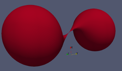
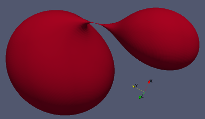
Figure 2: Color online. Slices through the event horizon at the exact point of merger to within numerical accuracy. Upper panel: Equal-mass non-spinning 16-orbit inspiral, Run 1 of Table 1, at $t/M=3902.897$; the point of merger is $t_{\rm merger}/M=3902.897\pm 0.006$. Here M is the sum of the ADM masses. Lower panel: Generic merger, Run 2 of Table 1, at $t/M=117.145$; the point of merger is $t_{\rm merger}/M=117.145\pm 0.005$. The error estimates come from the time resolution of our event horizon finder (i.e. our EH finder time step is $\sim 0.005M$); note that the merger occurs at the same time (within this error bound) for both medium and high resolutions of the numerical relativity simulations. At earlier times the two black hole horizons are disjoint. No toroids are evident in the limit of our accuracy.

Figure 2 shows the event horizons from two numerical simulations of binary black hole coalescence, at the time of merger. In the top panel, the two black holes start in a quasicircular orbit, and have equal masses and initially zero spins; details of this simulation were published in Ref. M. Scheel, M. Boyle, T. Chu, L. Kidder, K. Matthews and H. Pfeiffer (2009). The bottom panel shows a fully generic situation: again the black holes start in a quasicircular orbit, but the mass ratio is 2:1, and the initial spins have magnitude $a/M\simeq 0.4$ and are not aligned with each other or with the initial orbital plane. This simulation is “case F” of Ref. Szilagyi et al. (2009). For both of these simulations, we find the generators of the event horizon using the “geodesic method” of Cohen et al. (2009). We integrate generators backwards in time, and when we find that generators leave the event horizon, either through caustics (as determined by the vanishing of the local area element of the surface of generators Cohen et al. (2009)) or through crossover points (as determined by the method described in Section II) we flag them as having left the horizon. Figure 2 plots only those generators that are on the horizon at the time of merger. In both the equal-mass and generic cases, our results show that the event horizons merge at a point, with no intermediate toroidal phase to the limit of our numerical accuracy.

IV Topological structure of the Event Horizon for inspiraling and merging black holes

   

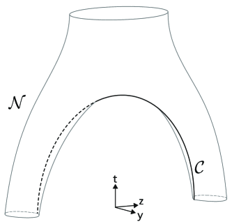
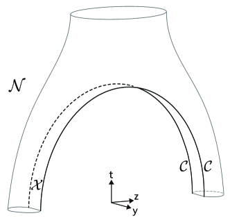
Figure 3: Diagrams of the event horizon null hypersurface in axisymmetric and non-axisymmetric mergers. The merger is along the z-axis. In both panels, the regions ${\cal C}\cup{\cal X}$ are spacelike. Left panel: In the axisymmetric case, the caustic/crossover set is reduced to a single line of caustic points, the “inseam” of the “pair of pants,” labeled ${\cal C}$. The $x$ direction is suppressed but, since the $x$ and $y$ directions are identical for axisymmetry, the diagram would be unchanged if we were to suppress $y$ in favor of $x$. Right panel: In the non-axisymmetric case, such as an inspiral (where we have “unwound” the legs of the “pair of pants” by going to a corotating frame), the set of crossover points ${\cal X}$ is two-dimensional, bounded on both sides by “inseams” ${\cal C}$. Unlike the axisymmetric case, here the $x$ and $y$ directions are not identical. Since the caustic/crossover set of points is a 2-surface, the diagram we would obtain by suppressing $y$ in favor of $x$ would look identical to the left panel, except that the single “inseam” would be composed of crossover points.

In order to understand why no toroidal intermediate stage is found in our simulations, we need to further understand the topological structure of the event horizon null hypersurface in the case of a binary inspiral and merger. In Husa and Winicour (1999), Husa and Winicour consider two sets of points. One set, labeled ${\cal C}$, is the set of all caustic points in the spacetime where neighboring event horizon geodesics cross. The other set of points, ${\cal X}$, is the set of all crossover points in the spacetime, where non-neighboring event horizon geodesics cross. They show that the set of points ${\cal X}$ is an open 2-surface on the event horizon null hypersurface ${\cal N}$, and that this set is bounded by the caustic set ${\cal C}$. They further show that the behavior of this 2-surface of caustic/crossover points is governed by the topology of the merger. In an axisymmetric prolate merger (such as our headon case), the 2-surface is reduced by the symmetry, resulting in the single boundary line of caustic points we see as being the “inseam” of the “pair of pants,” as shown in the left panel of Figure 3. In the non-axisymmetric case, the set of caustic and crossover points is a 2-surface on the event horizon, as shown in the case of a binary black hole inspiral in the right panel of Figure 3 (where we show the merger in a corotating frame).

The question of whether toroidal horizons can be found in the intermediate stages of binary black hole merger can be answered by considering the various ways in which these “pair of pants” diagrams can be sliced. The fact that the set caustic/crossover points ${\cal C}\cup{\cal X}$ is a spacelike 2-surface on a non-axisymmetric event horizon hypersurface (and, for an axisymmetric case, the line of points ${\cal C}$ is a spacelike line) provides some freedom in the allowed spacelike slicings of this surface.

   

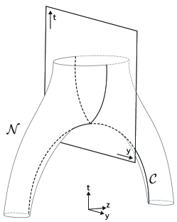
Figure 4: A 2-dimensional slice through the event horizon null hypersurface in an axisymmetric merger. The horizontal direction in the right panel could be either $x$ or $y$. We attempt to construct a slice ${\cal S}_{1}$ in $x$ (or $y$) from point ${\cal P}$ that intersects the black hole. This slice is clearly not spacelike. Since ${\cal N}$ is spacelike only at ${\cal C}$, only a slice such as ${\cal S}_{0}$ that does not intersect the black hole can be both spacelike and pass through ${\cal P}$.

Let us first consider whether a nontrivial topology might be obtained in the axisymmetric case. In order to do so, we need to consider how such a slice may be constructed. Clearly, if we were to construct “horizontal” spatial slices of the null hypersurface in the left panel of Figure 3, we would produce a slicing in which the merger occurred at a point. However, we can attempt to construct slices in which the lapse is somewhat retarded near the “crotch.” In Figure 4 we examine a 2-dimensional slice in $\{t,y\}$ through the center of the hypersurface. It is clear that if we choose a central point for the slice before the merger of the black holes, we cannot extend a spacelike slice from this central point in either the $x$ or $y$ directions in such a way as to encounter the black holes. Only in the $z$ direction can we encounter the black holes.

   

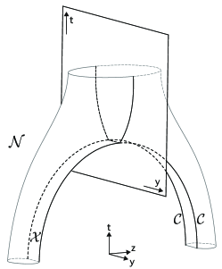
Figure 5: A 2-dimensional slice through the event horizon null hypersurface in a non-axisymmetric merger. Unlike the previous figure, the horizontal direction in the right panel is not interchangeable between $x$ and $y$. We construct three slices ${\cal S}_{0},{\cal S}_{1},{\cal S}_{2}$ from the starting point ${\cal P}$. These slices intersect the event horizon in different ways. Since ${\cal C}\cup{\cal X}$ is spacelike, all these slices are spacelike. Although exaggerated for effect, the tangent to ${\cal X}$ in the $t$-$y$ plane becomes null at ${\cal C}$ (see Shapiro et al. (1995)).

This changes however, when we consider the non-axisymmetric case. In this case, the $x$ and $y$ directions are different, as shown in the right panel of Figure 3. In Figure 5 we show a $\{t,y\}$ 2-slice of the event horizon. The event horizon is spacelike both at ${\cal C}$, and along the line ${\cal X}$. Thus, given a point ${\cal P}$ below the “crotch” of the event horizon, we can construct three distinct slices, each with different behavior. Slice ${\cal S}_{0}$ does not encounter the event horizon at all in the $y$ direction. Slice ${\cal S}_{1}$ encounters the event horizon four times: twice in the null region, and twice in the spacelike region. Finally, slice ${\cal S}_{2}$ encounters the event horizon four times in the spacelike region. Note that in the $x$ direction, the slice through the event horizon is identical to slice ${\cal S}_{0}$ of Figure 4 (except that the “inseam” is part of the crossover set ${\cal X}$ instead of the caustic set ${\cal C}$). Therefore, if we slice our spacetime using slices ${\cal S}_{1}$ or ${\cal S}_{2}$, our slice encounters the event horizon four times in the $z$ and $y$ directions, and not at all in the $x$ direction. This is precisely a toroidal intermediate stage. Such slices can be seen in three dimensions $\{t,y,z\}$ in Figure 6.

We now consider what the event horizon looks like in three spatial dimensions $\{x,y,z\}$ on each of the slices ${\cal S}_{0}$, ${\cal S}_{1}$, or ${\cal S}_{2}$ of Figures 5 and 6. The top panel of Figure 7 shows the intersection of the event horizon with the slice ${\cal S}_{0}$. Compare with Figure 6, which shows the same slice in the dimensions $\{t,y,z\}$. The slice ${\cal S}_{0}$ does not encounter the event horizon in the $x-y$ plane; this plane lies between the two black holes. On each black hole, the slice ${\cal S}_{0}$ encounters the two-dimensional crossover set ${\cal X}$ along a one-dimensional curve, and this curve is bounded by two caustic points from the set ${\cal C}$.

In contrast, the intersection of the event horizon with the slice ${\cal S}_{1}$ is shown in the middle panel of Figure 7. Compare with Figure 6, which shows the same slice in the dimensions $\{t,y,z\}$. This is a toroidal cross section of the horizon. Slice ${\cal S}_{1}$ intersects the event horizon four times along the $y$ axis: the outer two points are in the null region of the horizon ${\cal N}$ and the inner two are in the spacelike crossover set ${\cal X}$. Note that the inner edge of the torus is made up entirely of crossover points from the set ${\cal X}$ and does not include caustic points nor points in the set ${\cal N}$. The existence of an isolated set of crossovers that cannot be connected to caustics is a key signature of a toroidal horizon.

The bottom panel of Figure 7 shows the intersection of the event horizon with the slice ${\cal S}_{2}$, which is shown in the $\{t,y\}$ directions in Figure 5. This slice also produces a torus. Slice ${\cal S}_{2}$ intersects the event horizon four times along the $y$ axis, and each of these intersections is a crossover point in ${\cal X}$. As was the case for slice ${\cal S}_{1}$, the inner edge of the torus for slice ${\cal S}_{2}$ also consists entirely of crossover points. The outer edge of the event horizon intersects the two-dimensional crossover set ${\cal X}$ along two one-dimensional curves, and each of these curves is bounded by caustic points on each end.

It is important to note another distinction between the behavior of slices ${\cal S}_{1}$ and ${\cal S}_{2}$ in Figures 5 and 7. When a slice intersects the event horizon at a point that is a member of ${\cal C}\cup{\cal X}$, that point is the point where two generators of the event horizon pass through each other as they merge onto the event horizon. Consequently, that point is not a smooth part of the event horizon. If instead the slice intersects the event horizon at a point not in ${\cal C}\cup{\cal X}$, that point is a smooth part of the event horizon. Therefore, ${\cal S}_{1}$ corresponds to a toroidal intermediate stage where the torus has a non-smooth (i.e. sharp) inner edge and a smooth outer edge, and ${\cal S}_{2}$ corresponds to a stage where both the outside and the inside of the torus are sharp-edged. There also exists the possibility of a slice that looks like ${\cal S}_{1}$ in the positive $y$ direction and looks like ${\cal S}_{2}$ in the negative $y$ direction or vice versa; on such a slice the outer edge of the torus will be sharp on one side and smooth on the other.

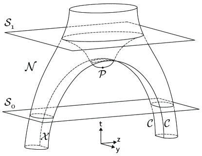
Figure 6: A 3-dimensional representation of slices ${\cal S}_{0}$ and ${\cal S}_{1}$ from Figure 5. Here we see the continuation of each slice in the $z$ direction. The event horizon is toroidal on slice ${\cal S}_{1}$; the center of the torus is ${\cal P}$. The toroidal region is the part of ${\cal S}_{1}$ that has dipped through the crossover region ${\cal X}$.

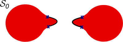
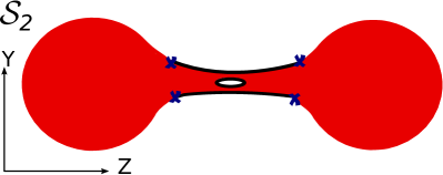
Figure 7: Color online. Cartoon illustrations of spatial slices ${\cal S}_{0}$, ${\cal S}_{1}$, and ${\cal S}_{2}$ of Figures 5 and 6. Null generators currently on the horizon are in red; linear sets of crossovers merging onto the horizon are indicated by black lines, and the location of caustic points are denoted by blue $X$s.

V Topological Structure of Simulated Event Horizons

Having shown how an appropriate choice of slicing yield spatial slices in which the event horizon is toroidal, we now hope to convince the reader that, up to the limit of our numerical resolution, we see no signs of a toroidal event horizon in the slicing of our simulations. In greater generality, we would like to answer the following question: What is the structure of caustic and crossover points for the simulations we have performed, and how do those results relate to the structure discussed in the previous section?

We can use Figure 6 to predict the structure of caustic and crossover points for an early slice through the event horizon of a non-axisymmetric merger. Unlike the axisymmetric case, where all geodesics merge onto the event horizon at a point, an early slice of the non-axisymmetric merger, say slice ${\cal S}_{0}$ in Figure 6, should show each black hole with a linear cusp on its surface, through which geodesics merge onto the horizon. The cusp should be composed of crossover points, except that the boundaries of the cusp should be caustic points. At a later time, the two black holes will merge, and whether or not a torus is formed depends on how the slice intersects the set of caustics and crossovers, as seen in Figure 7.

To clarify let us first state a precise condition for the presence or absence of a toroidal event horizon: A slice without a toroidal event horizon has the following property: For every crossover point on the horizon, there exists a path from that crossover point to a caustic point, such that the path passes through only crossover points (cf. Figure 7). For a slice with a toroidal event horizon, there exist crossover points on the horizon that are disconnected from all caustics, in the sense that no path can be drawn along crossovers that reaches a caustic. For example, in slices ${\cal S}_{1}$ and ${\cal S}_{2}$ of Figure 7, the crossover points on the inner edge of the torus are disconnected from all caustics.

A slicing of spacetime where the event horizon is never toroidal will appear like slice ${\cal S}_{0}$ at early times. Approaching merger, the two disjoint crossover sets will extend into “duck bill” shapes and then meet at a point, forming an “X” shape at the exact point of merger. After merger, the crossover set will then disconnect and will look like the outer edges of the horizon of slice ${\cal S}_{2}$ (with no torus in the middle). At even later times, each disjoint crossover set on the outer edge of the horizon will shrink to a single caustic point and then disappear.

A slicing of spacetime in which the event horizon is toroidal will also look like slice ${\cal S}_{0}$ at early times. But at times approaching merger, the disjoint crossover sets will meet at two (or more) points instead of one. If these meeting points are the caustics, then just after merger these caustics will disappear, leaving a ring of crossovers, and the horizon will look like slice ${\cal S}_{1}$ of Figure 7. If instead these meeting points are crossover points, then the crossover set will form a double “X” shape at merger, and after merger, the crossovers in the middle will form a ring, and the horizon will look like slice ${\cal S}_{2}$ of Figure 7. In this latter case, each disjoint crossover set on the outer edge of the horizon will eventually shrink to a single caustic point and then disappear. Furthermore, the central ring of crossovers will eventually shrink to a single point and disappear. If the disappearance of the crossovers on the horizon edge occurs before the disappearance of the central ring of crossovers, then for some time the horizon will look like slice ${\cal S}_{1}$ of Figure 7.

Comparing these predictions with the results of a simulation of finite numerical resolution requires care, since single points (such as the point of merger or the single caustic points that bound the crossover sets) cannot be found with infinite precision. We will discuss these limitations in the concluding paragraphs of this section. Let us now analyze the two numerical simulations studied here in detail.

V.1 Equal-mass non-spinning merger

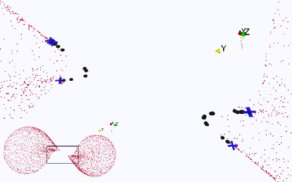
Figure 8: Color online. A snapshot of the geodesics being followed by the event horizon finder at time $t/M=t_{\rm merger}/M-0.067$, for the equal-mass inspiral. The small dots are geodesics currently on the event horizon. The larger points, either crosses or circles, represent geodesics in the process of merging onto the event horizon. Crosses represent points merging through caustic points, while circles represent points merging through crossovers. In this slice, the cusp on the black hole is linear, and composed of crossover points with caustics at the end points.

In Figures 8–10, we examine our simulation of the coalescence of two equal-mass non-spinning black holes. This simulation clearly displays the characteristics of a non-axisymmetric merger: the black holes do indeed have linear cusps on their surfaces, and we find caustic points occuring at the edges of the cusps.

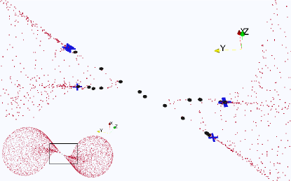
Figure 9: Color online. A snapshot of the geodesics being followed by the event horizon finder at time $t/M=t_{\rm merger}/M$, the exact point of merger (to within numerical error) in the equal-mass inspiral simulation. Labels are the same as in Figure 8. Although finding the exact point of merger is difficult given limited numerical time accuracy, we can extrapolate the “X” shape of the cusps to see that the merger point is clearly a crossover point.

Figure 8 shows generators before the point of merger. At this time, our slicing is consistent with slices parallel to ${\cal S}_{0}$ in Figure 5. These slices correspond to late enough times that they have encountered the horizon’s linear cusps but early enough times that they have not yet encountered points ${\cal C}$ in Figure 5. The event horizon slices show a “bridge” extending partway between the black holes, with cusps along each side. Each cusp is a line of crossover points on one of the black holes, anchored at each end by a caustic point.

At the precise point of merger (Figure 9) our slicing remains consistent with slices parallel to ${\cal S}_{0}$ in Figure 5. In this figure, slices parallel to ${\cal S}_{0}$ encounter the crossover region at slightly earlier times than they encounter the caustic lines. Therefore, at merger, the slice will intersect the horizon at one point (a crossover point) in the $y$ direction, and this point is where the linear cusps on the individual black holes meet. Consequently, the slice at the point of merger is expected to have a rough “X” shape of crossover points, meeting at the merger point, and anchored at the edges of the black hole cusps by caustic points. In Figure 9, we see that this is indeed the case. Note that if our slicing were similar to slice ${\cal S}_{1}$ in Figure 5 rather than slice ${\cal S}_{0}$, the linear cusps of the individual black holes would meet at two points rather than one, and these two points would be the caustic points at the boundary of the cusps. Similarly, if our slicing were similar to slice ${\cal S}_{2}$ in Figure 5, the cusps on the individual black holes would again meet at two points, and these would be crossover points. According to Figure 5, presumably there should exist slicings in which the two black holes would first touch at multiple points and form horizons of arbitrary genus.

After merger, the “X” shape of the merger has disconnected, resulting in two line segments of crossover points still bounded by caustics. This is clearly visible in Figure 10.

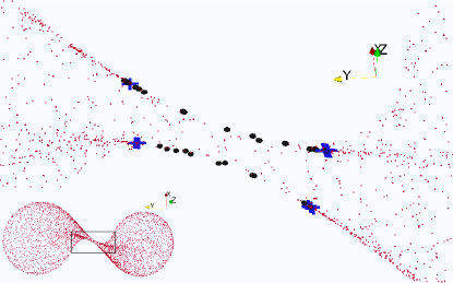
Figure 10: Color online. A snapshot of the geodesics being followed by the event horizon finder at time $t/M=t_{\rm merger}/M+0.039$, shortly after merger, for the equal-mass inspiral. Labels are the same as in Figure 8. The “bridge” between the two black holes has two lines of merger points running on either side of it, with the majority being crossover points anchored by caustics at either end.

Note that in Figures 8–10, we sometimes find multiple caustic points at the edge of the crossover set, rather than a single caustic point; this appears to be an effect of the finite tolerance of the algorithm that we use to identify caustic points. Similarly, we sometimes find caustic points that are slightly outside the crossover set, as in Figure 10. This too appears to be a finite-resolution effect. For the generic run below, we will present horizon figures computed with different number of geodesics in order to better understand this effect.

V.2 2:1 mass ratio with ‘randomly’ oriented spins

Here we examine in detail the topological structure of a generic binary black hole merger, Run 2 of Table 1. As noted earlier, this simulation corresponds to “case F” of Ref. Szilagyi et al. (2009). We use the term ‘generic’ to highlight the fact that this simulation lacks degeneracies in the parameter space of possible binary black hole mergers. While the equal-mass non-spinning simulation is symmetric in the masses and spin parameters of the black hole, and therefore has a few spatial symmetries, this generic simulation possesses no such symmetries. Even though the Kerr parameter $a/M$ of both holes is the same, their spin angular momenta differ by a factor of 4 due to their mass difference.

The lack of symmetries for the generic binary black hole configuration make it more difficult to detect or exclude the presence of a torus. To see this, consider one of the symmetries of the equal-mass merger: a rotation by $\pi$ about the direction of the orbital angular momentum. Because of this symmetry, the horizon finder needs to use only half the number of geodesics that would be required for a generic run: for every geodesic that is integrated backwards in time, another geodesic (with a position rotated by $\pi$ along the direction of the orbital angular momentum) is effectively obtained ‘for free’. Conversely, for a run without symmetries, it is necessary to use far more geodesics in the event horizon finder.

We will now examine the event horizon of the ‘generic’ merger at several spacetime locations that are important to the topological structure of the event horizon. Again, contrast this to the equal-mass merger, where there is only one spacetime region of interest to the topology of the horizon: the region and location where the common event horizon is first formed, and the associated cusp on the individual horizons.

For each of these spacetime locations we have investigated the consistency of the observed topological structure for several different numerical resolutions; specifically, we have run our event horizon finder using different spatial and temporal resolutions for the 2 + 1 event horizon hypersurface, as well as on two of the different resolutions used to evolve the 3 + 1 generic binary black hole merger simulation. We find no qualitative differences between the resolutions. In particular, though there appear to be features where a crossover point exists beyond the boundary or ‘anchor’ of a caustic, these features are not convergent with resolution. That is, upon going from a lower to higher resolution, it is possible to find an ‘anchoring’ caustic point for the apparently anomalous crossover. See Figure 12 for a clear demonstration of this phenomenon.

In the following sections, we examine the effect of two different spatial resolutions of our EH finder using a fine time resolution with a $\Delta t$ of $0.005M^{*}$: one resolution with $2(119+1)^{2}$ geodesics ($L=119$), and a higher spatial resolution using $2(191+1)^{2}$ geodesics ($L=191$). Here $M^{*}$ is nearly the total mass of the black holes on our evolution grid, $M$; $M^{*}=M/1.06157$ where $M$ is the the sum of the Christodoulou masses of the black holes; we use this notation here as all detailed event horizon calculations are done before scaling with the Christodoulou masses. Though we do not show them here, the results from the event horizon finding using a different time step, and from using a different background simulation resolution can be found online at www.black-holes.org/onToroidalHorizonsData.html. Also included at that location are detailed instructions on how to visualize the data in the same way in which we present it in this paper onT .

V.2.1 Pre-merger: $t=124.200M^{*}$

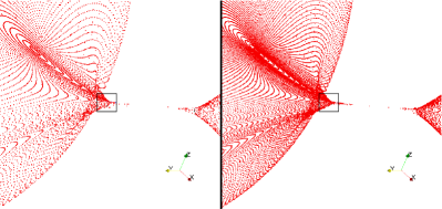
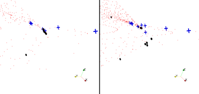
Figure 11: Color online. Generators of the event horizon at $t=124.200M^{*}$ . Current generators are shown as red points, and generators that are in the process of merging onto the event horizon are shown either as blue crosses (caustics), or larger black dots (crossovers). The left panel is computed using an apparent horizon finder resolution of of $L=119$, and the right panel uses a resolution of $L=191$. The lower panels are successive enlargements of the upper panels, focusing on the cusp near the larger black hole.

First, we examine the structure of the cusps on each black hole’s individual event horizons at a time before merger. Figure 11 displays a screenshot of this for two spatial resolutions used, focusing on the cusp on the larger black hole. Note that the resolution displayed here is much higher than in the equal-mass non-spinning case, and that we need to plot a much smaller region than in Figures 8–10 in order to visualize the structure of the cusp. Unfortunately, the topological structure of the event horizon is not as clearly discernible as in the equal-mass non-spinning case. A close examination of the data in 3D using the free visualization software ParaView par reveals that there do not appear to be any ‘isolated sets’ of crossovers, i.e. crossovers not anchored by caustics. It is very difficult to make this clear using static screenshots in a standard article, and so we have made the visualization data available publicly for inspection at www.black-holes.org/onToroidalHorizonsData.html, and encourage the curious reader to view the cusp in 3D onT .

Figure 12 displays the cusp on the smaller black hole at the same time. Here, one can clearly see an example of the limits of our current method of discretization of the event horizon surface: while we cannot see proper ‘anchoring’ caustics using a resolution of $L=119$ (left), we find the expected ‘anchoring’ caustics using higher resolution ($L=191$, right). To the limit of the $2+1$ resolution of our event horizon surface, we find only one connected set of crossovers on each black hole near their respective cusps.

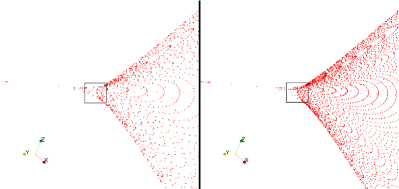
Figure 12: Color online. Same as the lower panels of Figure 11, except focusing on cusp on the smaller black hole.

V.2.2 Merger: $t=124.355M^{*}$

Our second time of interest occurs at the merger of the individual event horizons. Figure 13 illustrates the merger by showing screenshots of the coalescing bridge at three consecutive time steps. At merger, the black points indicating crossovers appear to form a “fat X” with finite width at the center, however this is likely a limitation of our finite temporal resolution; crossover points can only be flagged as as such if they join the horizon sometime between two time steps. In the limit of infinite spatial and temporal resolution, we would expect the same merger behavior as in the equal-mass non-spinning merger; i.e., the crossovers will be topologically one dimensional and form an “X” shape at merger (albeit a horizontally squished “X”). As in the equal-mass case, the point of merger occurs at a crossover.

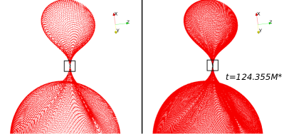
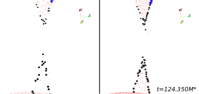
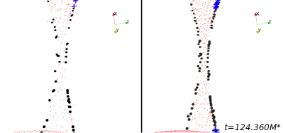
Figure 13: Color online. Same color coding and resolutions as in Figure 11, except shown at times very close to and surrounding the merger. Merger is localized to between times $t=124.355M^{*}$ and $t=124.360M^{*}$ (bottom row). The left side of each frame displays resolution $L=119$, and the right side of each frame shows resolution $L=191$.

V.2.3 Post-merger: $t=124.400M^{*}$

Finally, we focus at a time after merger: when the final geodesics join horizon (or, in the backwards-in-time language of event horizon finding, when the first geodesics leave the horizon). Figure 14 shows the common bridge between horizons, along with two linear cusps anchored by caustics. The asymmetry of the simulation is clear here: the cusp to the right of the bridge is closing faster than the cusp on the left. The cusp on the left is closing in the direction along the bridge because caustics on either side are approaching each other, and it is closing in the transverse direction because the locus of crossovers is shrinking and moving out from the center of the bridge. As we follow this picture further in time, the cusp on the right displays the same qualitative behavior.

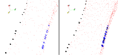
Figure 14: Color online. Same as Figure 11 but at time $t=124.400M^{*}$. The crossover set on the left side of the bridge connecting the holes extends past the extents of the lower screenshot and is bounded by caustics that are outside the view of the frame. Also, on the right edge of the bridge, note the extended line of caustics and the presence of crossovers between the caustics. This appears to be the effect of finite resolution in the event horizon finder, since the appearance is different in the right and left panels. Such numerical phenomena suggest the need for advanced techniques such as adaptive refinement of geodesic placement if we wish to completely resolve event horizon features at a reasonable computational cost.

V.3 Discussion on the numerical analysis of topological features

Figures 11–14 illustrate why it is difficult to formulate a precise numerical condition that tells us the scale to which we can exclude the presence of a toroidal structure; in the generic case, it is difficult at times to say that we have even identified all connected components of the set of crossovers and caustics visually and qualitatively. In particular, though the distribution of geodesics is well spaced on the spherical apparent horizon at late times (which serves as the initial data for our event horizon finder), this does not ensure a uniform distribution of geodesics on the event horizon surface at earlier times. Thus, as one can see in Figure 14, the crossover points are not uniformly distributed along the line of the cusp. How do we know these crossover points are of the same connected component? Remember, if the crossover points in this region are members of at least two distinct connected components, and there are no “anchoring” caustic points in their neighborhood, it would indicate the presence of a toroidal event horizon! Runs at different resolutions indicate that our visual and qualitative identification of the crossover and caustic structure is consistent with a single linear cusp, but the structure is still only resolved up to the largest separation of crossover points in the cusp. We note that the implementation of adaptive geodesic placement in our event horizon finder is likely necessary to resolve these sorts of issues. We therefore choose to postpone the issue of a quantitative and precise bound on the scale to which we can exclude a toroidal event horizon to future work.

It is clear, however, from these results that our simulation is consistent with the topological structure discussed by Husa and Winicour in Husa and Winicour (1999), and outlined in Section IV above. Our slicing corresponds to slices parallel to ${\cal S}_{0}$ in Figures 4–6 through the structure of the event horizon, but this does not preclude the possibility of other spacelike slicings producing toroidal intermediate stages during merger.

VI Conclusion

In this work, we have taken the first steps in examining the topological structure of event horizons in generic binary black hole merger simulations. We focus on determining the topology of the two dimensional event horizon surface as it appears on spacelike slices of numerical relativity simulations. In particular, we concentrate on the presence or absence of a toroidal event horizon, as previous work Husa and Winicour (1999); Siino (1998a, b) has suggested that the existence of a toroidal horizon should appear generically in non-axisymmetric mergers of black holes. In order to sharpen the discussion on toroidal horizons, we examine the caustic and crossover structure of the event horizon from a theoretical (Sec IV) and numerical (Sec V) point of view. Following Husa and Winicour Husa and Winicour (1999), we emphasize the distinction between caustic points, where neighboring (infinitesimally separated) geodesics cross and join the horizon, and crossover points, where geodesics separated by a finite angle cross and join the horizon. Note that the union of caustics and crossovers are the ‘crease set’ discussed in the work of Siino Siino (1998a, b). We now would like to recount the main topics we have discussed:

1. First, in Sections I–III we have described improvements in our event horizon finding code and summarized the topological results for event horizons found from SpEC binary black hole mergers. We describe our algorithm (which scales like ${\cal O}(N^{2})$ where $N$ is the number of horizon generators) to detect crossover points, and we find that the computational cost is not prohibitive for finding the event horizons of binary black hole mergers.

2. In Section IV, we reviewed the caustic and crossover structure of the event horizons of binary black hole mergers for the axisymmetric and generic cases. Concentrating on spatial slicings that result in toroidal event horizons, we diagram slices of the event horizon in multiple spatial and temporal directions in order to elucidate the caustic and crossover structure present in the cases of toroidal and non-toroidal event horizons.

3. Subsequently, in our introduction to Section V, we have discussed a necessary condition for a spatial slice of the event horizon surface to be toroidal: the existence of a maximally path-connected set of crossover points that is disconnected from all caustic points.

4. Finally, we presented a detailed analysis of the event horizons found numerically from two inspiraling binary black hole simulations. We find in all cases that the intersection of the event horizon with any of our constant-time spatial hypersurfaces is topologically spherical rather than toroidal. Despite the lack of toroids, the structure of caustics and crossovers in our simulations are consistent with Husa & Winicour Husa and Winicour (1999). We paid particular attention to analyzing the generic merger for consistency when varying several different numerical resolutions. Though only two resolutions are compared in this paper, we have made public the visualization data for all four resolutions of the generic merger that we examined onT . We encourage the reader to view at least one of our data sets in 3D, as this is perhaps the most powerful way to gain insight into the behavior of the event horizons from our simulations.

For the simulations presented here, it is difficult to compute a precise upper limit on the size of any tori that might exist in the exact solution but are too small for us to detect in the simulations. The main reason for this difficulty is that our ability to resolve features of the event horizon depends not only on the numerical resolution used to solve Einstein’s equations, but also on the resolution of the algorithm used to find and classify event horizon generators. The latter resolution dominates in the examples presented here. This is because in our current method, the geodesics are located on a fixed computational mesh that is chosen at the beginning of the backwards-in-time geodesic integration (i.e. at late times). We suggest that the best way to tackle this issue would be to devise an event horizon finding algorithm with iterative or adaptive geodesic resolution and placement. Thus, one could build into the adaptive method a target precision with which to resolve caustic and crossover sets. Though challenging, such an approach would allow one to investigate the topological structure of numerical event horizons to a much higher precision, while also providing a solid quantitative measure of the precision to which features are resolved.

Before we conclude, we would like to discuss a few important open questions about how the slicing condition used in our numerical simulations relates to the topological structure of the observed spatial cross sections of the event horizon: 1) Can an existing simulation be re-sliced to produce a toroidal cross section of the event horizon? 2) Alternatively, could the gauge conditions of our generalized harmonic evolution code be modified in order to produce a binary black hole merger in a spatial slicing with a toroidal event horizon? 3) Why have recent numerical simulations of merging black holes not produced slicings with a toroidal horizon when it has been thought that an intermediate toroidal phase should be relatively generic? The answer to the first question is clearly ‘yes’. Previous work in the literature Husa and Winicour (1999); Siino (1998a, b); Shapiro et al. (1995) shows that it is possible to have a spacelike slicing of a dynamical event horizon with a toroidal topology, and that the question of whether the horizon is toroidal depends on how the spacelike slice intersects the spacelike crossover set ${\cal X}$, as we review in Section IV.

Questions 2) & 3), however, are far more mysterious and are ripe for future investigation. Is the lack of toroids in our simulations endemic to the types of foliations used in numerical relativity as a whole, or just to the generalized harmonic Lindblom et al. (2006); Lindblom and Szilágyi (2009); Szilagyi et al. (2009) gauge conditions we currently use in the SpEC code? It would be interesting to see if a toroidal event horizon phase could be produced from the same initial data used in our current simulations by modifying gauge conditions in such a way as to retard the lapse function near the merger point of the black holes. So far our attempts to do so have been unsuccessful. Hence, it has been speculated that some property of those numerical gauge choices that yield stable binary black hole evolutions also avoids slicings in which the event horizon is toroidal.