Dynamics of bright solitons and soliton arrays in the nonlinear Schrödinger equation with a combination of random and harmonic potentials

Abstract

We report results of systematic simulations of the dynamics of solitons in the framework of the one-dimensional nonlinear Schrödinger equation (NLSE), which includes the harmonic-oscillator (HO) potential and a random potential. The equation models experimentally relevant spatially disordered settings in Bose-Einstein condensates (BECs) and nonlinear optics. First, the generation of soliton arrays from a broad initial quasi-uniform state by the modulational instability (MI) is considered, following a sudden switch of the nonlinearity from repulsive to attractive. Then, we study oscillations of a single soliton in this setting, which models a recently conducted experiment in BEC. Basic characteristics of the MI-generated array, such as the number of solitons and their mobility, are reported as functions of the strength and correlation length of the disorder, and of the total norm. For the single oscillating soliton, its survival rate is found. Main features of these dependences are explained qualitatively.

I Introduction

The interplay of the disorder and nonlinearity is a topic which has been attracting a great deal of interest for a long time, see reviews review -review3 . In particular, much work has been done on the analysis of dynamics of solitons in disordered external potentials, chiefly in one-dimensional settings, see, e.g., Refs. soliton1 -review4 and references therein. These studies find an important application to the description of Bose-Einstein condensates (BECs) trapped in random potentials. The latter topic was addressed in many theoretical BEC0 -BEC6 and experimental Randy1 -Randy3 works.

A ubiquitous theoretical model used in this field is the nonlinear Schrödinger equation, NLSE (alias the Gross-Pitaevskii equation, in terms of BEC GPE ) for the wave function $u(x,t)$, which includes a regular trapping potential and a term accounting for a disordered potential. The normalized form of this equation, with scaled time $t$ and space coordinate $x$, is

$$iu_{t}+\frac{1}{2}u_{xx}+g|u|^{2}u-\frac{1}{2}{\Omega}^{2}x^{2}u-V_{\mathrm{dis}}(x)u=0,$$ (1)

where $g=+1$ and $-1$ correspond to the self-attractive and self-repulsive nonlinearities, both signs being possible in BEC, $\Omega$ characterizes the strength of the harmonic-oscillator (HO) trapping potential, and $V_{\mathrm{dis}}(x)$ is a random potential  representing the spatial disorder. In particular, this model describes dipole oscillations of the trapped condensate, experimentally studied in recent work Randy3 , where strong effective dissipation induced by the disordered potential was discovered. On the other hand, Eq. (1) with $t$ replaced by the propagation distance coordinate $z$ is a model of a nonlinear optical waveguide with a random perturbation of the local refractive index, which is represented by the disordered potential review0 , hence the results reported below apply to spatial solitons in the nonlinear waveguide as well.

Our objective is to systematically investigate fundamental properties of solitons in the framework of the model based on Eq. (1). These include the formation and motion of soliton trains due to the modulational instability (MI) of the broadly distributed condensate, and, as suggested by the experiment reported in Ref. Randy3 , oscillations of a single soliton which is originally placed at a distance from the minimum of the trapping potential, $x=0$. The results for these two types of the dynamical behavior, based on systematic simulations of Eq. (1) and averaging over many realizations of the random setting, as well as on a qualitative analysis of the observed effects, are reported, respectively, in Sections II and III, and the paper is concluded by Section IV.

II Formation of soliton arrays by the modulational instability in the spatially disordered environment

The subject of this Section is the effect of the spatial disorder on the formation of soliton chains from an initial quasi-uniform state, and the subsequent evolution of the chains. The numerical simulations were subject to the following specifications. The spatial domain was taken as $-60\pi<x<+60\pi$, and the trapping strength is $\Omega^{2}=25\times 10^{-4}$, hence the respective HO length is much smaller than the size of the integration domain, which makes it possible to consider multi-soliton trains, and persistent motion of the solitons. The split-step Fourier method with a spatial grid composed of $1024$ points and time step $\Delta t=0.001$ was employed for the spatial and temporal discretization of Eq. (1). The total integration time is $T=80$. A fourth-order optimized implementation of the splitting was used, as in Refs. Blanes02 ; Montesinos05 . Further, the disorder was represented by a spatially correlated random function, $V_{\mathrm{dis}}(x)=V_{d}f(x,\theta)$, where $V_{d}$ is the strength of the disorder, and the marginal distribution of $f(x,\theta)$ has an exponential form, its covariance function being $C(x_{1},x_{2})=\exp(-2(x_{1}-x_{2})^{2}/V_{z}^{2})$, in which $V_{z}$ is the correlation length. Other type of random functions as in Yaglom can be considered in a similar way.

The initial quasi-uniform distribution of the condensate is taken as the ground-state solution of Eq. (1) with the self-repulsive nonlinearity, i.e., with $g=-1$, in the form of $u=\exp\left(-i\mu t\right)U(x)$, where $\mu$ is the real chemical potential, and function $U(x)$ was found as a stationary solution of the associated nonlinear diffusion equation (the imaginary-time version imaginary of Eq. (1)):

$$u_{t}=\frac{1}{2}u_{xx}-|u|^{2}u-\frac{1}{2}\Omega^{2}x^{2}u-V_{\mathrm{dis}}(x)u+\mu u.$$ (2)

The same split-step method was used to solve Eq. (2). Then, the evolution of the MI (modulational instability) of this state was simulated in real time, following a sudden switch of the self-repulsion into self-attraction, i.e., replacement of $g=-1$ by $g=+1$ in Eq. (1), which exactly corresponds to the reversal of the sign of the nonlinearity by means of the Feshbach resonance in the well-known BEC experiment of Randy .

The MI splits the initial quasi-uniform state into a chain of solitons, which, generally speaking, is an obvious outcome of the evolution induced by the reversal of the nonlinearity sign. However, a new aspect of this outcome, on which we focus here, is the effect of the disordered environment on the resulting solitary wave chain. We have collected results which demonstrate the dependence of the characteristics of the emerging soliton chain on three control parameters: strength $V_{d}$ and correlation length $V_{z}$ of the random potential, and the total norm of the initial state, $N=\int_{-\infty}^{+\infty}|u(x)|^{2}dx$. The characteristics whose variation was monitored are (i) the number of solitons; (ii) the largest displacement of solitons, i.e., the largest distance that peaks of individual solitons can travel in the course of the evolution; Basically the displacement for each soliton is computed as the distance between its leftmost and rightmost positions. Then the largest displacement is simply the largest value among all the solitons. (iii) the normalized average kinetic energy per soliton, which is defined as

$$\bar{K}=\left(\sum M_{j}\right)^{-1}\left(\sum\frac{1}{2}M_{j}v_{j}^{2}\right),$$ (3)

where the summation is performed on the full set of solitons in the emerging configuration, $v_{j}$ is the velocity of the $j$-th soliton, and $M_{j}=\int|u(x)|^{2}dx$ is its effective mass, with the integration performed over a vicinity of the solitary wave’s peak where the local amplitude of the field exceeds half of its peak value.

The results presented below were produced by averaging over 100 different random realizations. Note that this leads to a non-integer number as the number of solitons for most cases. Typical examples of the realizations are displayed in Figs. 1 and 2, for small and large correlations lengths, $V_{z}=5$ and $V_{z}=25$, respectively. Individual solitons can be easily identified in the plots.

   

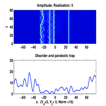
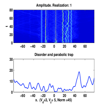
Figure 1: (Color online) Two realizations of the random multi-soliton configuration generated by the development of the modulational instability for $V_{z}=5$. Here and in the next figure, top plots depict the spatiotemporal evolution of $|u(x,t)|$, while the bottom ones display the corresponding total potential—the sum of the HO trap and the random part.

   

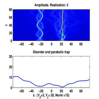
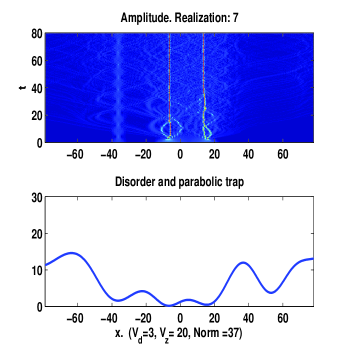
Figure 2: (Color online) Two realizations of the random multi-soliton patterns for $V_{z}=20$

The results for the number of solitons in emerging pattern and their largest displacement are summarized in Figs. 3 - 5. In each panel, we fix two of the above-mentioned control parameters ($V_{d},V_{z},N$) and vary the third one. For example, the norm is varied in Fig. 3, each curve corresponding to a particular set of values of $V_{d}$ and $V_{z}$.

   

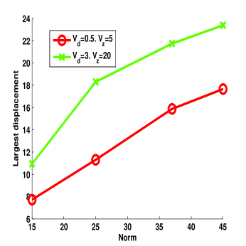
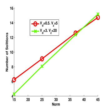
Figure 3: (Color online) Results obtained for fixed strength and correlation length of the disorder, while the total norm varies. Here and in the two following figures, the left and right panels display, respectively, the largest displacement of solitons, and the number of solitons in the final configuration produced by the simulations.

   

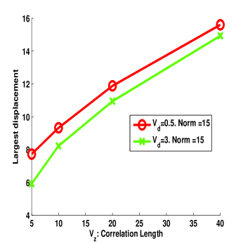
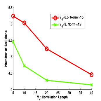
Figure 4: (Color online) The results for fixed total norm and strength of the disorder.

   

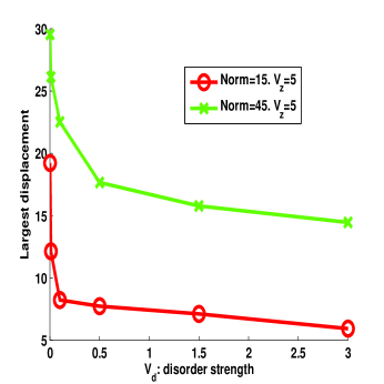
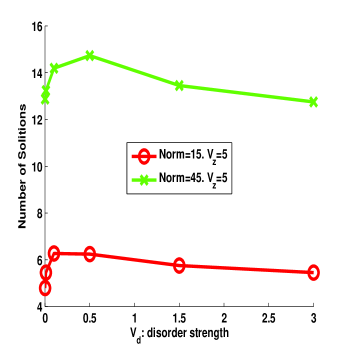
Figure 5: (Color online) The results for fixed total norm and correlation length of the disorder.

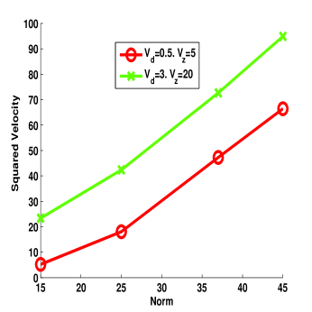
Figure 6: (Color online) The variation of the mean kinetic energy with increase of the total norm.

The following conclusions can be made from Figs. 3 - 5.

1. According to Fig. 3, the number of solitons in the chain increases linearly with the total norm, so that the mean norm per soliton, $N_{\mathrm{sol}}$, is approximately constant. This is a direct effect of trapping the wave field by the random potential: in free space, the entire condensate tends to coalesce into a single soliton, which corresponds a minimum of the system’s Hamiltonian Zakharov . However, the sufficiently strong disorder pins portions of the fragmented condensate, forcing them to self-trap into separated solitons. A fundamental threshold condition for the self-trapping of an initial state into an NLS soliton is known in the form of the condition imposed on the area of the initial configuration Zakharov :

   $$S\equiv\int_{-\infty}^{+\infty}|u_{0}(x)|dx>S_{0}\equiv\ln\left(2+\sqrt{3}\right)\approx 1.32.$$ (4)

   For fixed parameters of the disorder, i.e., fixed average width $\bar{L}$ of local potential wells trapping fragments of the condensate, the above-mentioned constancy of the norm-per-soliton, $N_{\mathrm{sol}}$, implies a constant average amplitude, $\bar{A}\sim\sqrt{N_{\mathrm{sol}}/\bar{L}}$, hence the average area per soliton is constant too, $\bar{S}\sim\bar{A}\bar{L}\sim\sqrt{N_{\mathrm{sol}}\bar{L}}$, which is consistent with condition (4), that also implies an approximately constant area per soliton. Thus, condition (4) may explain the results observed in Fig. 3.

2. Figure 3 demonstrates the increase of both the largest distance traveled by the solitons, and their mean kinetic energy, with the increase of the total norm. This feature may be explained by the fact that an individual soliton, moving through the disordered potential, is strongly braked due to the emission of radiation review . The effectively dissipative character of the motion of coherent wavepackets in this setting was recently demonstrated in the experiment of Randy3 (see also the following Section). However, if the system is filled by the trapped condensate, the moving soliton actually interacts with trapped segments of the condensate, i.e., with an effective pseudopotential review4 , which is essentially smoother than the “bare” random potential. This effect leads to the suppression of the radiation losses, allowing the solitons to be more mobile.

3. Figure 4 shows that the soliton number decreases, while the largest displacement increases, as the correlation length of the disorder, $V_{z}$, increases. This conclusion is consistent with the conclusions presented in the previous item, as the increase of $V_{z}$ implies the transition to a less disordered potential.

4. Figure 5 clearly shows that both the soliton number and largest displacement change very rapidly when $V_{d}$ increases from zero to small finite values, i.e., the disorder starts to kick in when its strength is quite small. The observed jump of the soliton number to larger values, and the simultaneous drop of the free-path length are consistent with the above argument which states that a deeper random potential splits the condensate into a large number of solitons, and impedes their free motion.

III Oscillations of the soliton in the combined potential

Our next objective is to simulate the oscillatory motion of a single soliton in the combined HO an random potentials, which parallels the recently reported experiment performed in the condensate of ⁷Li Randy3 . While the latter experiment focused on the repulsive interaction case of the (dissipative in the presence of disorder) dipolar motion of a full condensate, it is straightforward to envision such dynamics for an attractive interaction condensate, namely a localized solitary wave. For this purpose, simulations of Eq. (1) were run with parameters selected as the rescaled version of those dealt with in the experiment, where the total number of atoms was $\simeq 10000$, the scattering length $a_{s}$ is taken as three times the Bohr radius of ⁷Li, the transverse trapping frequency is $\omega_{r}=2\pi\times 260$ Hz, and the longitudinal one is $\omega_{z}=2\pi\times 5.5$ Hz. The initial conditions were taken as $u_{0}(x)=\sqrt{2a_{\mathrm{IC}}}{\rm sech}(\sqrt{2a_{\mathrm{IC}}}(x-x_{0}))$, where $x_{0}$ is the initial shift of the soliton from the bottom of the HO potential, and $a_{\mathrm{IC}}$ is determined by the total number of atoms. With the above physical values, $\Omega^{2}=4.4749\times 10^{-4}$ and $a_{\mathrm{IC}}=0.2269$ were used in the simulations. The split-step Fourier method was employed in this case too, with a sufficiently small spacing in order to properly resolve the size of the soliton. In the course of the simulations, the disorder in Eq. (1) was turned on after one and a quarter of the period of the oscillations of the soliton in the HO potential, i.e., when the soliton’s center was passing the origin, $x=0$.

For given initial shift $x_{0}$, we mainly varied two parameters (as before), the correlation length $V_{z}$ and disorder strength $V_{d}$. For each fixed value of $V_{z}$, we varied $V_{d}$ to infer whether the soliton would survive after 10 periods of the oscillations. The goal was to compute the survival rate of the soliton under the influence of the disorder, using 10 realizations for this purpose. In each realization, the survival of the soliton was registered if its final norm, integrated over the FWHM range around its center, exceeded $50\%$ of the initial value in the same range. The survival rate is then defined as the number of realizations featuring the surviving soliton, divided by 10 (the total number of the realizations). Typical examples of the survival and destruction of the oscillating solitons are displayed in Fig. 7. [Note that $h$ in the horizontal axis label denotes the Planck constant].

   

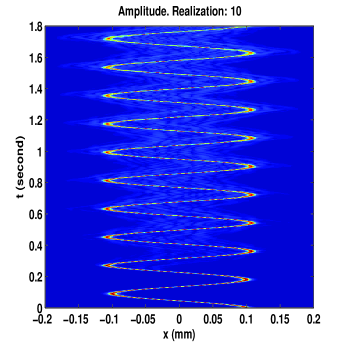
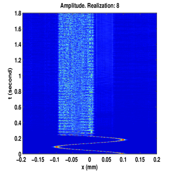
Figure 7: (Color online) The left and right panels display examples of solitons which, respectively, survive and get destroyed in the course of the oscillations, for an initial shift of the soliton to $x_{0}=0.1~{}$mm, its FWHM width $9.2142~{}\mathrm{\mu}$m, and a disorder correlation length of $V_{z}=9.4264~{}\mathrm{\mu}$m. The disorder strength corresponding to the left and right panels is, respectively, $V_{d}=h\cdot 5$(Hz) and $h\cdot 180$(Hz), where $h$ is the Planck constant.

The results for $x_{0}=0.6$ and $0.1$ mm are displayed in Figs. 8 and 9. They correspond to the dimensionless values of $x_{0}=254.6$ and $42.4$ in Eq.(1). These clearly indicate that the survival rate drops to zero as the disorder strengthens and the correlation length decreases, in agreement with the experimental observations for the repulsive case Randy3 . This is a natural consequence of the increasing rate of the emission of radiation by the soliton oscillating across the random potential.

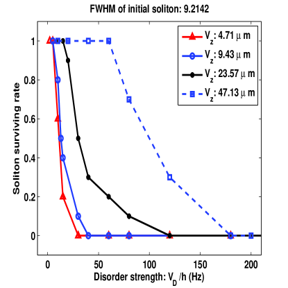
Figure 8: (Color online) The survival rate of the oscillating soliton for initial shift $x_{0}=0.6$ mm.

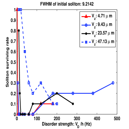
Figure 9: (Color online) The survival rate of the oscillating soliton for $x_{0}=0.1$ mm.

When the disorder becomes very strong, the soliton starts to survive again, as seen in Fig. 9 for $x_{0}=0.1$ mm. This is explained by the fact that a very strong random potential consists of local potential wells which quickly trap and immobilize the soliton, preventing its decay into radiation and, in addition, the strong random potential impedes the separation of the radiation waves from the parent soliton. The restabilization boundary is shown in Fig. 10. The approximately linear dependence of the minimum disorder strength, necessary for the restabilization, on $x_{0}$ can be explained with the help the above argument: the driving force acting on the soliton in the HO potential grows linearly with $x_{0}$, while the largest pinning force, induced by the random potential, is proportional to $V_{d}$. Therefore, the equilibrium between the two, which determines the restabilization threshold, implies $V_{d}\sim x_{0}$.

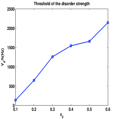
Figure 10: (Color online) For given initial shift $x_{0}$, the soliton survives if the disorder strength, $V_{d}$, exceeds the minimum value shown in this plot.

IV Conclusions

The objective of this work was to report results of a systematic numerical analysis of individual soliton and soliton train dynamics in the experimentally relevant setting based on the 1D NLSE including the combination of the HO (harmonic-oscillator) and random potentials. This setting may be realized in BEC and nonlinear optics. Two basic problems were considered: the generation of soliton trains from the initial quasi-uniform state by the MI (modulational instability), after the sudden switch of the nonlinearity from the self-repulsion into attraction, and the survival or decay of a single soliton oscillating in this combined potential. Dependences of the main characteristics of the soliton train, and of the survival rate of the single oscillating soliton, on the strength and correlation length of the disordered potential, and also dependences of the characteristics of the soliton array on the total norm of the initial state, have been produced by averaging over a large number of random realizations. Salient features of this dependences have been explained in a qualitative form.

A challenging problem is extending the analysis to the 2D setting, which may suggest new possibilities for the experiment. There, one has to consider the interplay of the above analyzed mechanisms with the potential collapse type events of super-critical atomic blobs and hence the relevant phenomenology will be considerable richer. The 2D setting is also of interest for the repulsive interaction dynamical case, whereby the formation of dark solitons and trains thereof reported in Randy3 may be substituted by the formation of vortices and vortex streets.

Acknowledgment: The first author’s work was supported in part by the National Science Foundation under the grant DMS-1016047. The second author was supported by the National Science Foundation under the grant DMS-0806762 and by the Alexander von Humboldt Foundation.

References

- (1) Kivshar Y S and Malomed B A, Dynamics of solitons in nearly integrable systems, 1989, Rev. Mod. Phys. 61 763.
- (2) Gredeskul S A and Kivshar Y S, Propagation and scattering of nonlinear waves in disordered systems, 1992, Phys. Rep. 216 1-61.
- (3) Belitz D and Kirkpatrick T R, The Anderson-Mott transition, 1994, Rev. Mod. Phys. 66 261-390.
- (4) Hennig D and Tsironis G P, Wave transmission in nonlinear lattices, 1999, Phys. Rep. 307, 333-432.
- (5) Evers F and Mirlin A D, Anderson transitions, 2008, Rev. Mod. Phys. 80 1355-1417.
- (6) Scharf R and Bishop A R, Length-scale competition for the one-dimensional nonlinear Schrödinger equation with spatially periodic potentials, 1993, Phys. Rev. B 47 1375-1383.
- (7) Alexeeva N V, Barashenkov I V, and Tsironis G P, Impurity-induced stabilization of solitons in arrays of parametrically driven nonlinear oscillators, 2000, Phys. Rev. Lett. 84 3053-3056.
- (8) Pertsch T, Peschel U, Kobelke, J Schuster K, Bartelt H, Nolte S, Tünnermann A, and Lederer F, Nonlinearity and disorder in fiber arrays, 2004, Phys. Rev. Lett. 93 053901.
- (9) Schwartz T, Bartal G, Fishman S, and Segev M, Transport and Anderson localization in disordered two-dimensional photonic lattices, 2007 Nature 446 52-55.
- (10) Kartashov Y V, Malomed B A and Torner L, Solitons in nonlinear lattices, 2011, Rev. Mod. Phys. 83 247-305.
- (11) Wang D W, Lukin M D, and Demler E, Disordered Bose-Einstein condensates in quasi-one-dimensional magnetic microtraps, 2004, Phys. Rev. Lett. 92 076802.
- (12) Paul T, Leboeuf P, Pavloff N, Richter K, and Schlagheck P, Nonlinear transport of Bose-Einstein condensates through waveguides with disorder, 2005, Phys. Rev. A 72 063621.
- (13) Schulte T, Drenkelforth S, Kruse J, Ertmer W, Arlt J, Sacha K, Zakrzewski J, and Lewenstein M, Routes towards Anderson-like localization of Bose-Einstein condensates in disordered optical lattices, 2005, Phys. Rev. Lett. 95 170411.
- (14) Shapiro B, Expansion of a Bose-Einstein condensate in the presence of disorder, 2007, Phys. Rev. Lett. 99 060602.
- (15) Akkermans E, Ghosh S, and Musslimani Z H, Numerical study of one-dimensional and interacting Bose-Einstein condensates in a random potential, 2008, J. Phys. B: At. Mol. Opt. Phys. 41 045302.
- (16) Albert M, Paul T, Pavloff N and Leboeuf P, Dipole oscillations of a Bose-Einstein condensate in the presence of defects and disorder, 2008, Phys. Rev. Lett. 100 250405.
- (17) Fishman S, Krivolapov Y and Soffer A, On the problem of dynamical localization in the nonlinear Schrödinger equation with a random potential, 2008, J. Stat. Phys. 131 843-865.
- (18) Chen, Y P, Hitchcock J, Dries D, Junker M, Welford C, Pollack S E, Corcovilos T A, and Hulet R G, Phase coherence and superfluid-insulator transition in a disordered Bose-Einstein condensate, 2008, Phys. Rev. A 77 033632.
- (19) Chen, Y P, Hitchcock J, Dries D, Junker M, Welford C, Pollack S E, Corcovilos T A, and Hulet R G, Experimental studies of Bose-Einstein condensates in disorder, 2009, Physica D 238 1321-1325.
- (20) Dries D, Pollack S E, Hitchcock J M and Hulet R G, Dissipative transport of a Bose-Einstein condensate, 2010, Phys. Rev. A 82 033603.
- (21) Pitaevskii L P and Stringari A 2003 Bose-Einstein Condensation (Clarendon Press, Oxford).
- (22) Montesinos G D and Pérez-García V M, Numerical studies of stabilized Townes solitons, 2005 Math. Comput. Simul. 69 447-456.
- (23) Blanes S and Moan P C, Practical symplectic partitioned Runge-Kutta and Runge-Kutta-Nystrom methods, 2002, J. Comp. Appl. Math. 142 313-330.
- (24) Yaglom A M 2004 Introduction to the Theory of Stationary Random Functions (Dover Phoenix Editions ) .
- (25) Chiofalo M L, Succi S, and Tosi M P, Ground state of trapped interacting Bose-Einstein condensates by an explicit imaginary-time algorithm, 2000, Phys. Rev. E 62 7438-7444.
- (26) Strecker K E, Partridge G B, Truscott A G and Hulet R G, Formation and propagation of matter-wave soliton trains, 2002, Nature 417 150-153.
- (27) Zakharov V E, Manakov S V, Novikov S P and Pitaevskii L P 1984 Theory of Solitons: the Inverse Scattering Method (Consultants Bureau, New York) .