Testing Inflation with Dark Matter Halos

Abstract

Cosmic inflation provides a mechanism for generating the early density perturbations that seeded the large-scale structures we see today. Primordial non-Gaussianity is among the most promising of few observational tests of physics at this epoch. At present non-Gaussianity is best constrained by the cosmic microwave background, but in the near term large-scale structure data may be competitive so long as the effects of primordial non-Gaussianity can be modeled through the non-linear process of structure formation. We discuss recent work modeling effects of a few types of primordial non-Gaussianity on the large-scale halo clustering and the halo mass function. More specifically, we compare analytic and N-body results for two variants of the curvaton model of inflation: (i) a “$\tau_{NL}$” scenario in which the curvaton and inflaton contribute equally to the primordial curvature perturbation and (ii) a “$g_{NL}$” model where the usual quadratic $f_{NL}$ term in the potential cancels, but a large cubic term remains.

I Introduction

From the anisotropies in the cosmic microwave background (CMB) to the large-scale distribution of dark matter halos hosting galaxies, the universe appears rich with structure. A central goal of observational cosmology is to understand the period of inflation that is believed to have generated this structure Guth and Pi (1982); Hawking (1982); Starobinsky (1982); Bardeen et al. (1983). Current CMB data confirms inflationary predictions for a spatially flat universe with primordial curvature perturbations drawn from a nearly scale-invariant power spectrum Komatsu et al. (2011). Nevertheless, distinguishing between microphysical models remains a challenge.

Evidence for non-Gaussianity in the primordial perturbations could rule out large classes of inflationary models and shed light on the mechanism that generated the initial structure (see e.g. Bartolo et al. (2004); Chen (2010)). At present the most stringent bounds on primordial non-Gaussianity come from CMB experiments Komatsu et al. (2011); Fergusson et al. (2010); Smidt et al. (2010), but data from galaxy surveys is increasingly competitive (see, e.g. Slosar et al. (2008); Carbone et al. (2010); Shandera et al. (2010)). In these proceedings we give an overview of analytic and N-body results for the abundance and clustering of dark matter halos with local non-Gaussian initial conditions described by the parameters $f_{\rm NL}$, $g_{\rm NL}$ and $\tau_{NL}$. In §II we introduce three examples of non-Gaussian initial conditions. In §III we review analytic models of the impact of local non-Gaussian initial conditions on the abundance and clustering of dark matter halos. Comparison of the analytic models and results from N-body simulations is given §IV. In §V we summarize our results. The reader is referred to the original references Smith and LoVerde (2010); LoVerde and Smith (2011); Smith et al. (2011a, b) for a more detailed discussion.

II Examples of local non-Gaussian statistics: $f_{\rm NL}$, $g_{\rm NL}$, $\tau_{NL}$

If the initial curvature perturbations are homogeneous, isotropic and Gaussian their statistics are entirely characterized by the two point correlation function, or power spectrum

$$\langle\Phi({\bf k})\Phi({\bf k^{\prime}})\rangle=(2\pi)^{3}\delta_{{\rm Dirac}}({\bf k}+{\bf k^{\prime}})P_{\Phi\Phi}(k)\,.$$ (1)

If $\Phi$ has any non-zero odd $N$-point function or even $N$-point function that just isn’t specified by the two-point function (i.e. $\langle\Phi({\bf x}_{1})\Phi({\bf x}_{2})\dots\Phi({\bf x}_{N})\rangle\neq\langle\Phi({\bf x}_{1})\Phi({\bf x}_{2})\rangle\langle\Phi({\bf x}_{3})\Phi({\bf x}_{4})\rangle\dots\langle\Phi({\bf x}_{N-1})\Phi({\bf x}_{N})\rangle+{\rm permutations}$) then $\Phi$ is non-Gausssian.

While there are an abundance of inflationary scenarios producing a variety of non-Gaussian initial conditions (there are some organizing principles; see for example Babich et al. (2004)) here we focus on initial curvature that can be written as a non-linear mapping of a Gaussian random field that is local in real space. These types of initial conditions can arise in the curvaton model Linde and Mukhanov (1997); Lyth and Wands (2002). For a general review of inflationary scenarios giving local non-Gaussian initial conditions see Byrnes and Choi (2010).

II.1 $f_{\rm NL}$

Consider defining the initial curvature as a Gaussian random field $\Phi_{G}$, plus a small ($\mathcal{O}(f_{\rm NL}\sqrt{\langle\Phi_{G}^{2}\rangle})$) fractional perturbation Komatsu and Spergel (2001)

$$\Phi_{NG}({\bf x})=\Phi_{G}({\bf x})+f_{\rm NL}\left(\Phi_{G}^{2}({\bf x})-\langle\Phi_{G}^{2}\rangle\right)\,.$$ (2)

The new field $\Phi_{NG}({\bf x})$ obeys non-Gaussian statistics. In particular it has a skewness $\langle\Phi_{NG}^{3}\rangle\sim 6f_{\rm NL}\langle\Phi_{G}^{2}\rangle^{2}$, and kurtosis $\langle\Phi_{NG}^{4}\rangle_{c}\equiv\langle\Phi_{NG}^{4}\rangle-3\langle\Phi_{NG}^{2}\rangle^{2}\sim 48f_{\rm NL}^{2}\langle\Phi_{G}^{2}\rangle^{3}$. The CMB constraints on this form of primordial non-Gaussianity are $-10<f_{\rm NL}<74$ at $95\%$ confidence Komatsu et al. (2011).

Another non-Gaussian feature is the coupling between different physical scales. We can gain some insight into the mode coupling by splitting the Gaussian field into “short” and “long” wavelength pieces, $\Phi_{G}=\Phi_{G,s}+\Phi_{G,l}$. The short wavelength fluctuations of the non-Gaussian field depend on both short and long wavelength modes of the Gaussian field,

$$\Phi_{NG,s}=\Phi_{G,s}+f_{\rm NL}\left(\Phi_{G,s}^{2}-\langle\Phi_{G,s}^{2}\rangle\right)+2f_{\rm NL}\Phi_{G,s}\Phi_{G,l}\,.$$ (3)

In particular, an observer on top of a long wavelength mode $\Phi_{G,l}$ will see small-scale statistics that depend on the value of $\Phi_{G,l}$

$$\left.\langle\Phi_{NG,s}^{2}\rangle\right|_{l}\sim\langle\Phi_{NG,s}^{2}\rangle\left(1+4f_{\rm NL}\Phi_{G,l}+4f_{\rm NL}^{2}\Phi_{G,l}^{2}\right)$$ (4)

$$\left.\langle\Phi_{NG,s}^{3}\rangle\right|_{l}\sim 6f_{\rm NL}\langle\Phi_{G,s}^{2}\rangle^{2}\left(1+4f_{\rm NL}\Phi_{G,l}\right)$$ (5)

where we have only kept terms up to $\mathcal{O}(f_{\rm NL}^{2})$. This coupling between short and long wavelength scales will be important to understand the impact of non-Gaussian initial conditions on the clustering of dark matter halos.

II.2 $g_{\rm NL}$

A variant on Eq. (2) is to consider a local mapping where the quadratic term vanishes, and the cubic term is important Okamoto and Hu (2002); Enqvist and Nurmi (2005)

$$\Phi_{NG}({\bf x})=\Phi_{G}({\bf x})+g_{\rm NL}\left(\Phi_{G}^{3}({\bf x})-3\Phi_{G}({\bf x})\langle\Phi_{G}^{2}\rangle\right)\,.$$ (6)

With this mapping the skewness of $\Phi_{NG}$ vanishes and the kurtosis is $\langle\Phi_{NG}^{4}\rangle_{c}\sim 24g_{\rm NL}\langle\Phi_{G}^{2}\rangle^{3}$. The CMB limits $-12.34<g_{\rm NL}/10^{5}<15.58$ at $95\%$ confidence Fergusson et al. (2010).

In the $g_{\rm NL}$ model, the coupling of short and long scales in Eq. (6) gives a small-scale variance that depends on $\Phi_{G,l}^{2}$,

$$\left.\langle\Phi_{NG,s}^{2}\rangle\right|_{l}\sim\langle\Phi_{NG,s}^{2}\rangle\left(1+6g_{\rm NL}\Phi_{G,l}^{2}\right)$$ (7)

and a local skewness the varies linearly with $\Phi_{G,l}$

$$\left.\langle\Phi_{NG,s}^{3}\rangle\right|_{l}\sim 18g_{\rm NL}\langle\Phi_{G,s}^{2}\rangle^{2}\Phi_{G,l}\,.$$ (8)

Comparing the leading terms in Eqs. (5) and (8), we see that to an observer sitting on a long wavelength mode $\Phi_{l}$, it appears that they live in a cosmology with $f_{\rm NL}^{eff}({\bf x})=3g_{\rm NL}\Phi_{G,l}({\bf x})$!

II.3 $\tau_{NL}$

Another variation is to consider initial curvature which is the sum of two fields $\phi_{G}$ and $\sigma_{G}$ which fluctuate independently ($\langle\phi_{G}\sigma_{G}\rangle=0$) but have proportional power spectra, $P_{\phi\phi}/P_{\sigma\sigma}\equiv\xi^{2}={\rm constant}$. Non-Gaussianity is generated by adding a term quadratic in $\sigma$,

$$\Phi_{NG}({\bf x})=\phi_{G}({\bf x})+\sigma_{G}({\bf x})+f_{\rm NL}(1+\xi^{2})^{2}\left(\sigma_{G}^{2}({\bf x})-\langle\sigma_{G}^{2}\rangle\right)\,.$$ (9)

The skewness in this model is given by $\langle\Phi_{NG}^{3}\rangle\sim 6f_{\rm NL}\langle\Phi_{NG}^{2}\rangle^{2}$, and the kurtosis is $\langle\Phi_{NG}^{4}\rangle_{c}\sim 48f_{\rm NL}^{2}(1+\xi^{2})\langle\Phi_{NG}^{2}\rangle^{3}\equiv 48\tau_{NL}\langle\Phi_{NG}^{2}\rangle^{3}/(\frac{6}{5})^{2}$ where the factor of $6/5$ is conventional. Current CMB bounds on this parameter are $-6000<\tau_{NL}<33,000$ at $95\%$ confidence Smidt et al. (2010).

In this $\tau_{NL}$ model, there is a coupling between small-scale fluctuations in $\Phi_{NG}$ and the long-wavelength fluctuations in $\sigma_{G}$

$$\left.\langle\Phi_{NG,s}^{2}\rangle\right|_{l}\sim\langle\Phi_{NG,s}^{2}\rangle\left(1+4f_{\rm NL}(1+\xi^{2})\sigma_{G,l}+4f_{\rm NL}^{2}(1+\xi^{2})^{3}\sigma_{G,l}^{2}\right)\,.$$ (10)

In this two-field example $\tau_{NL}\geq(\frac{6}{5}f_{\rm NL})^{2}$. One may wonder whether this inequality is fundamentally related to the physics of inflation. Suyama and Yamaguchi (2008) showed the inequality was true at tree-level using the $\delta N$ formalism. In fact, this inequality can be interpreted as a positivity constraint that must be satisfied regardless of the mechanism that generated the perturbations. A formal proof is given in Smith et al. (2011b), but the argument can be understood as follows. From Eqs. (4) & (10) we can see that $f_{\rm NL}$ is a measure of the large-scale correlation between the potential $\Phi$ and the locally measured small-scale power ($f_{\rm NL}\sim\langle\Phi_{l}\Phi_{s}^{2}\rangle/\langle\Phi_{l}^{2}\rangle\langle\Phi_{s}^{2}\rangle$). On the other hand, $\tau_{NL}$ is a measure of the large-scale variance in the small-scale power ($\tau_{NL}\sim\langle\Phi_{l}^{2}\Phi_{s}^{2}\rangle_{c}/\langle\Phi_{l}^{2}\rangle^{2}\langle\Phi_{s}^{2}\rangle$). The inequality $\tau_{NL}\geq(\frac{6}{5}f_{\rm NL})^{2}$ then arises as the condition that the correlation coefficient between the small-scale power and $\Phi$ must be between -1 and 1.

III Impact of non-Gaussian initial conditions on large-scale structure: analytic predictions

In the previous section we discussed non-Gaussianity in the initial curvature perturbation. To understand the impact of primordial non-Gaussianity on the abundance and clustering of dark matter halos, we need a model that relates halos to perturbations in the initial curvature. In linear theory, the matter density perturbation $\delta$ is simply related to the initial curvature,

$$\delta({\bf k},z)=\frac{2k^{2}T(k)D(z)}{3\Omega_{m}H_{0}^{2}}\Phi({\bf k})\equiv\alpha(k,z)\Phi({\bf k})$$ (11)

where $T(k)$ is the transfer function and $D(z)$ is the linear growth function. A simple prescription for halo formation is to smooth the linear density field on scale $M$

$$\delta_{M}({\bf x})\equiv\frac{1}{V}\int_{V\sim M/\rho_{m}}\!\!d^{3}{\bf x}^{\prime}\delta({\bf x}-{\bf x}^{\prime})$$ (12)

and to model halos of mass $>M$ as regions of the smoothed initial density field with $\delta_{M}({\bf x})>\delta_{c}$, where $\delta_{c}$ is the spherical collapse threshold. The probability distribution function (PDF) for fluctuations $\delta_{M}$ can be written in terms of the cumulants for the smoothed density fluctuation $\delta_{M}$

$$\sigma_{M}^{2}\equiv\langle\delta_{M}^{2}\rangle\,,\quad\kappa_{3}(M)\equiv\frac{\langle\delta_{M}^{3}\rangle}{\sigma_{M}^{3}}\,,\quad\kappa_{4}(M)\equiv\frac{\langle\delta_{M}^{4}\rangle_{c}}{\sigma_{M}^{4}}\,,\quad\dots$$ (13)

where $\kappa_{3}\propto f_{\rm NL}$ and $\kappa_{4}$ contains terms $\propto g_{\rm NL}$ and $\propto\tau_{NL}$. If $\delta_{M}$ is non-Gaussian, an infinite number of cumulants are needed to completely specify the PDF. However, one can approximate the PDF with a finite set of cumulants and for our purposes $\sigma_{M}^{2}$, $\kappa_{3}$ and $\kappa_{4}$ are sufficient.

In the next sections we use these elements to model the abundance and clustering of dark matter halos. In the plots throughout this paper we use the WMAP5+BAO+SN fiducial cosmology Dunkley et al. (2009): baryon density $\Omega_{b}h^{2}=0.0226$, cold dark matter (CDM) density $\Omega_{c}h^{2}=0.114$, Hubble parameter $h=0.70$, spectral index $n_{s}=0.961$, optical depth $\tau=0.080$, and power-law initial curvature power spectrum $k^{3}P_{\zeta}(k)/2\pi^{2}=\Delta_{\zeta}^{2}(k/k_{\rm piv})^{n_{s}-1}$ where $\Delta_{\zeta}^{2}=2.42\times 10^{-9}$ and $k_{\rm piv}=0.002$ Mpc^-1.

III.1 Halo abundance

Dark matter halos form from rare positive fluctuations in the matter density. Press & Schechter Press and Schechter (1974) gave a simple analytic model for the abundance of dark matter halos with mass $M$ in terms of the PDF for the linear matter density fluctuations smoothed on scale $R=(3M/4\pi\rho_{m})^{1/3}$,

$$n(M)=-2\frac{\rho_{m}}{M}\frac{\partial}{\partial M}\mathcal{P}(\delta_{M}>\delta_{c},M)$$ (14)

where $\delta_{c}\approx 1.68$ is the spherical collapse threshold and $\mathcal{P}(\delta_{M}>\delta_{c},M)$ is the probability for $\delta_{M}>\delta_{c}$. Using

$$\mathcal{P}_{{\rm Gaussian}}(\delta_{M}>\delta_{c},M)=\int_{\delta_{c}}^{\infty}d\delta_{M}\frac{1}{\sqrt{2\pi\sigma_{M}^{2}}}e^{-\frac{1}{2}\delta_{M}^{2}/\sigma_{M}^{2}}$$ (15)

in Eq. (14) gives the Press-Schechter mass function Press and Schechter (1974), which is known to disagree at the $\sim 50\%$ level with the mass function measured from N-body simulations Jenkins et al. (2001). Nevertheless, the expression in Eq. (14) has long been used to predict the relative abundance of halos in a non-Gaussian cosmology to a Gaussian one Lucchin and Matarrese (1988). Typically, the full non-Gaussian PDF is not known, but approximate expressions for $n(M)$ are obtained by truncating an asymptotic expansion (e.g. Matarrese et al. (2000)) or Edgeworth series (e.g. LoVerde et al. (2008) – hereafter the “Edgeworth mass function”) for the PDF and using Eq. (14). These expressions agree well with N-body simulations with $f_{\rm NL}$-type initial conditions provided the “modified” collapse threshold $\delta_{c}^{\prime}\approx 1.42$ is used (e.g. Pillepich et al. (2008)).

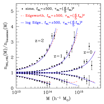
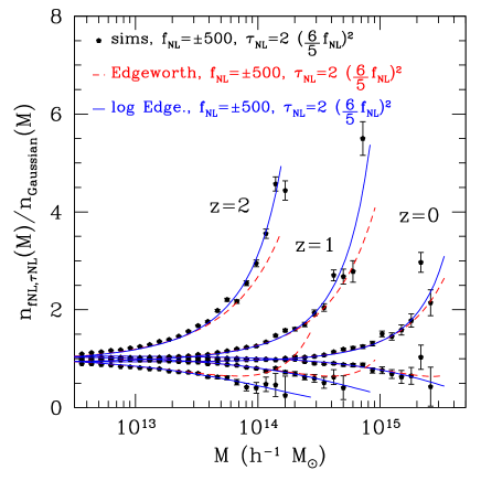
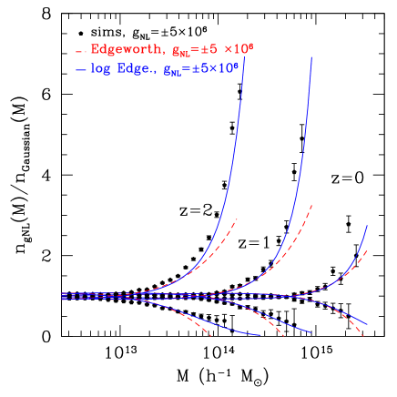
In LoVerde and Smith (2011), truncating the series for $\ln\mathcal{P}(\delta_{M}>\delta_{c},M)$ rather than $\mathcal{P}(\delta_{M}>\delta_{c})$ was proposed, where the Edgeworth expression is used for the PDF. In the limit of small non-Gaussian corrections, the mass function obtained this way (which we call the “log-Edgeworth” mass function) agrees with the Edgeworth mass function, but the in high-mass limit where non-Gaussian corrections are important, the “log-Edgeworth” mass function is better behaved (see Figs. (1) & (2)).

III.2 Scale-dependent halo bias from $f_{\rm NL}$ and $g_{\rm NL}$-type initial conditions

In the previous section we discussed modeling dark matter halos as regions where the linear density field $\delta_{M}$ exceeds $\delta_{c}$. If a fluctuation $\delta_{M}$ is sitting on top of a longer wavelength fluctuation in the density $\delta_{l}$, then the local collapse threshold is adjusted to $\delta_{c}-\delta_{l}$, thus the halo abundance fluctuates with the density as

$$\frac{\delta n({\bf x})}{n}=1+\left.\frac{\partial\ln n(M,\delta_{c}-\delta_{l})}{\partial\delta_{l}}\right|_{\delta_{l}=0}\delta_{l}({\bf x})\,,$$ (16)

where the $1$ accounts for the fact that the Eulerian halo number density is increased by a factor of $1+\delta$ with respect to the Lagrangian one given by $n(M)$.

As we’ve seen in §II non-Gaussian initial conditions can cause small scale statistics like the variance and skewness to be modulated by the long-wavelength potential $\Phi_{l}$. For the $f_{\rm NL}$ and $g_{\rm NL}$ initial conditions the small scale variance and skewness are modulated by $\Phi_{l}$. Accounting for this modifies Eq. (16) to

$$\frac{\delta n}{n}({\bf x})=1+\frac{\partial\ln n}{\partial\delta_{l}}\delta_{l}({\bf x})+4f_{\rm NL}\frac{\partial\ln n}{\partial\ln\sigma_{M}^{2}}\Phi_{l}({\bf x})+3g_{\rm NL}\frac{\partial\ln n}{\partial f_{\rm NL}}\Phi_{l}({\bf x})\,.$$ (17)

In Fourier space, the density field is related to the early-time gravitational potential through $\alpha(k,z)$ which allows us to write

$$\frac{\delta n}{n}({\bf k}) = \left(b+\frac{4f_{\rm NL}}{\alpha(k,z)}\frac{\partial\ln n}{\partial\ln\sigma_{M}^{2}}+\frac{3g_{\rm NL}}{\alpha(k,z)}\frac{\partial\ln n}{\partial f_{\rm NL}}\right)\delta_{l}({\bf k})$$ (18)

$$\equiv b_{f_{\rm NL},g_{\rm NL}}(k)\delta_{l}({\bf k})$$ (19)

where $b\equiv 1+\partial\ln n/\partial\delta_{l}$. We’ll refer Eq. (18) to as the “peak-background-split” (PBS) prediction for the scale-dependent non-Gaussian bias.

For a mass function dependent only on the combination $\delta_{c}/\sigma_{M}$, rather than $\delta_{c}$ and $\sigma_{M}$ separately, we can write the $\sigma_{M}^{2}$ derivative in terms of the constant bias $b$

$$\frac{\delta n}{n}({\bf k})=\left(b+\frac{2f_{\rm NL}\delta_{c}(b-1)}{\alpha(k,z)}+\frac{3g_{\rm NL}}{\alpha(k,z)}\frac{\partial\ln n}{\partial f_{\rm NL}}\right)\delta_{l}({\bf k})\,.$$ (20)

The $g_{\rm NL}$ bias coefficient can be rewritten in terms of $b$, but the expression is more complicated Smith et al. (2011a). The $f_{\rm NL}$ dependent bias above was first written down in Dalal et al. (2008), but the derivation given here follows that of Slosar et al. (2008). The expression for $g_{\rm NL}$ bias term is from Smith et al. (2011a), but see also Desjacques and Seljak (2010); Desjacques et al. (2011).

From Eq. (20) the large-scale halo-matter and halo-halo power spectra are given by

$$P_{hm}(k)=b_{f_{\rm NL},g_{\rm NL}}(k)P_{mm}(k)\quad{\rm and}\quad P_{hh}(k)=b_{f_{\rm NL},g_{\rm NL}}^{2}(k)P_{mm}(k)\,.$$ (21)

The analytic form for the $f_{\rm NL}$-dependence of $P_{hm}$ and $P_{hh}$ given by Eqs. (20) & (21) has been shown to be in excellent agreement with simulations (see e.g. Dalal et al. (2008); Grossi et al. (2009); Pillepich et al. (2008)). Using the scale dependent halo bias, Slosar et al. (2008) constrain $-29<f_{\rm NL}<70$ at $95\%$ confidence. Using the fact that the scale-dependent bias from $g_{\rm NL}$ has the same $k$-dependence ($\propto 1/\alpha(k,z)$), Desjacques and Seljak (2010) applied the $f_{\rm NL}$ constraints from Slosar et al. (2008) to limit $-3.5<g_{\rm NL}/10^{5}<8.2$.

III.3 Stochasticity between halos and dark matter from $\tau_{NL}\neq(\frac{6}{5}f_{\rm NL})^{2}$ initial conditions

For the two-field initial conditions given in §II.3, the linear density field is determined by the sum of the potentials $\sigma+\phi$, through

$$\delta({\bf k},z)=\alpha(k,z)\left(\phi({\bf k})+\sigma({\bf k})\right)\,,$$ (22)

but the small scale power is modulated by $4f_{\rm NL}(1+\xi^{2})\sigma_{l,G}$. So the number of halos fluctuates as

$$\frac{\delta n}{n}({\bf k})=b\delta_{l}({\bf k})+2f_{\rm NL}(1+\xi^{2})\delta_{c}(b-1)\sigma_{l}({\bf k})\,.$$ (23)

The halo-matter cross-power spectrum is unchanged from the $f_{\rm NL}$ case,

$$P_{hm}(k,z) = \left(b+\frac{2f_{\rm NL}\delta_{c}(b-1)}{\alpha(k,z)}\right)P_{mm}(k,z)$$ (24)

$$= b_{f_{\rm NL}}(k)P_{mm}(k,z)$$ (25)

but the halo-halo power spectrum is now

$$P_{hh}(k,z)=b_{f_{\rm NL}}^{2}P_{mm}(k,z)+4(\frac{25}{36}\tau_{NL}-f_{\rm NL}^{2})\delta_{c}^{2}(b-1)^{2}P_{\Phi\Phi}(k)\,.$$ (26)

The second term above represents stochasticity of the halo field with respect to the dark matter field Tseliakhovich et al. (2010).

IV Impact of non-Gaussian initial conditions on large-scale structure: comparison with simulations

To study the halo mass function and clustering, we performed collisionless $N$-body simulations using the GADGET-2 TreePM code Springel (2005). Simulations were done using periodic box size $R_{\rm box}=1600$ $h^{-1}$ Mpc, particle count $N_{p}=1024^{3}$, and force softening length $R_{s}=0.05(R_{\rm box}/N_{p}^{1/3})$. With these parameters and the fiducial cosmology from §III, the particle mass is $m_{p}=2.92\times 10^{11}$ $h^{-1}$ $M_{\odot}$. Non-Gaussian initial conditions were implemented by generating Gaussian fields and applying the maps in Eq. (2), Eq (6), or Eq. (9). The non-Gaussian fields were linearly evolved to the initial simulation redshift, $z=100$, using the transfer functions from CAMB Lewis et al. (2000). Halos were identified using the Friends of Friends algorithm Frenk et al. (1988) with linking length $L_{FoF}=0.2R_{box}N_{p}^{-1/3}$ and halo positions are identified using the mean of the particle positions. For further details see Smith and LoVerde (2010); LoVerde and Smith (2011); Smith et al. (2011a).

(a)	(b)

Figure 1: The non-Gaussian correction to the halo mass function. Plotted is $n_{NG}(M,z)/n_{G}(M,z)$ for (a) $f_{\rm NL}=\pm 500$, $\tau_{NL}=(\frac{6}{5}500)^{2}$, (b) $f_{\rm NL}=\pm 500$, $\tau_{NL}=2(\frac{6}{5}500)^{2}$

(a)	(b)

Figure 2: The non-Gaussian correction to the halo mass function. Plotted is (a) $f_{\rm NL}=0$, $g_{\rm NL}=\pm 5\times 10^{6}$. In panel (b) the non-Gaussian corrections for $(f_{\rm NL},\tau_{NL})=(500,(\frac{6}{5}500)^{2})$, $(f_{\rm NL},\tau_{NL})=(500,2(\frac{6}{5}500)^{2})$ and $g_{\rm NL}=5\times 10^{6}$ are plotted together for comparison.

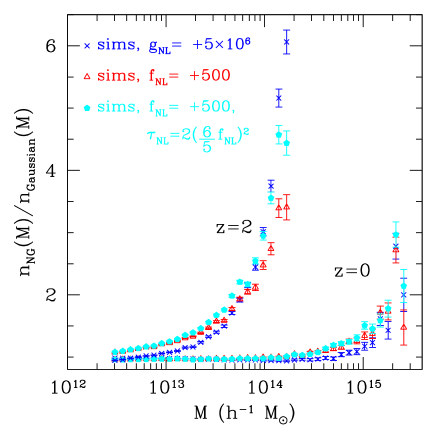
In Fig. (1) and Fig. (2) the ratio of the non-Gaussian mass function $n_{NG}(M)$ to Gaussian mass function $n_{G}(M)$ is plotted. The effects of primordial non-Gaussianity are clearly visible, positive (negative) $f_{\rm NL}$, $g_{\rm NL}$ increase (decrease) the abundance of halos, most significantly at high mass and high redshift. The curves show the analytic predictions for the Edgeworth and log-Edgeworth mass functions described in §III.1. In regions where the effects of non-Gaussianity are small, both are in reasonable agreement with the N-body results. However, at the high mass end where non-Gaussian effects are largest the log-Edgeworth mass function is clearly in better agreement.

In panel (b) of Fig. (2) the non-Gaussian corrections for ($f_{\rm NL}$, $\tau_{NL}=(\frac{6}{5}f_{\rm NL})^{2}$), ($f_{\rm NL}=0$, $g_{\rm NL}$) and ($f_{\rm NL}$, $\tau_{NL}=2(\frac{6}{5}f_{\rm NL})^{2}$), are plotted together. For $\tau_{NL}\neq(\frac{6}{5}f_{\rm NL})^{2}$, the non-Gaussian effects are clearly larger than in the $f_{\rm NL}$-only case. However, the mass and redshift dependence of the curves is similar: we found that models with $\tau_{NL}\geq(\frac{6}{5}f_{\rm NL})^{2}$ can be made to look like models with $\tau_{NL}=(\frac{6}{5}f_{\rm NL})^{2}$ by using a larger value of $f_{\rm NL}$. On the other hand, the mass dependence of $g_{\rm NL}$ effects is distinctly steeper at high masses, thus in principle primordial skewness and kurtosis may be distinguishable with the mass function.

(a)	(b)

Figure 3: (a) An example to illustrate that halo bias in a $g_{\rm NL}$ cosmology takes the functional form form $b(k)=b_{1}+\beta_{g}g_{\rm NL}/\alpha(k)$. This figure corresponds to redshift $z=0.5$ and halo mass range $1.15\leq M\leq 1.83\times 10^{14}$ $h^{-1}$ $M_{\odot}$, but we find the same functional form for all redshifts and halo masses. (b) The mass dependence of the $g_{\rm NL}$ bias, compared with the peak-background split prediction $3\frac{\partial\ln n}{\partial f_{\rm NL}}$, there is excellent agreement.

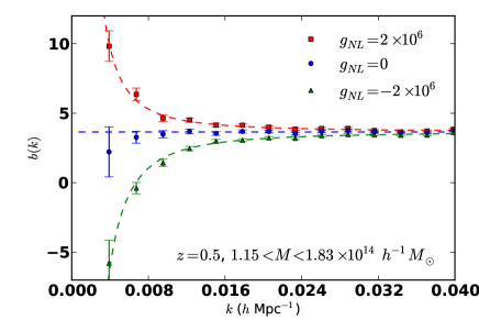
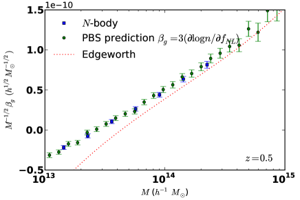
In Fig. (3) we show the scale-dependent bias from $g_{\rm NL}$ initial conditions. The $k$-dependence of the bias is accurately described by the form $b+g_{\rm NL}\beta_{g}/\alpha(k)$ where $\beta_{g}$ is a constant. In panel (b) we compare the peak-background split prediction $\beta_{g}=3g_{\rm NL}\partial(\log n)/\partial f_{\rm NL}$ with the value of $\beta_{g}$ measured from simulations. The agreement is excellent. Also shown is the analytic prediction for $3\partial(\log n)/\partial f_{\rm NL}$ using the Edgeworth mass function. At these masses the analytic form is not sufficiently accurate to describe the $g_{\rm NL}$ bias.

(a)	(b)

Figure 4: (a) An example to illustrate that halo bias in the two-field model of §II.3 with $\tau_{NL}=(1+\xi^{2})(\frac{6}{5}f_{\rm NL})^{2}$ is stochastic ($r_{ij}\neq 0$). This is in contrast to the Gaussian case and the $f_{\rm NL}$-only model given in §II.1, for which halo bias is non-stochastic on large-scales ($r_{ij}=0$). This figure corresponds to redshift $z=0.5$ and halo mass range $1.15\leq M\leq 1.83\times 10^{14}$ $h^{-1}$ $M_{\odot}$, but we find the same functional form for all redshifts and halo masses. (b) An example of the peak-background split prediction (solid curve) with the measured stochasticity – in this case the lowest-order peak-background split clearly over-predicts the stochasticity.

We now consider the stochasticity induced by initial conditions with $\tau_{NL}\neq(\frac{6}{5}f_{\rm NL})^{2}$. The stochasticity parameter is given by,

$$r_{ij}(k)=\frac{P_{h_{i}h_{j}}(k)-\delta_{ij}/n}{P_{mm}(k)}-\frac{P_{mh_{i}}(k)P_{mh_{j}}}{P_{mm}^{2}(k)}\,.$$ (27)

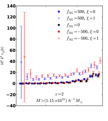
where $h_{i}$ stands for halos in the $i^{th}$ mass bin. Stochasticity is generally expected on small scales from the $1$-halo term in the halo power spectrum. But on large scales halos are expected to be non-stochastic tracers of the dark matter. In Fig. (4) we show that the stochasticity vanishes on large-scales for Gaussian initial conditions and $f_{\rm NL}$ initial conditions described by Eq. (2). On the other hand, the two field initial conditions described in Eq. (9) giving $\tau_{NL}\neq(\frac{6}{5}f_{\rm NL})^{2}$ do give rise to large-scale stochasticity.

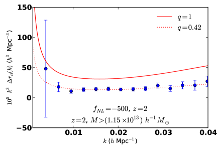
In panel (b), we show the scale dependence of the stochasticity in comparison with the lowest-order peak-background split prediction from §III.3. Here we find disagreement: the scale dependence of the analytic prediction agrees well with what is seen in simulations but the amplitude is too high by $\sim 50\%$. The disagreement between the amplitude of the stochasticity seen in simulations and the prediction from Eq. (26) varies with mass and redshift, but is typically $\sim 30\%$ Smith and LoVerde (2010). For Gaussian initial conditions, we also found inconsistent agreement between the halo model predictions for $r_{ii}$ and the measured values. This mismatch in $r_{ii}$ values is in qualitative agreement with Hamaus et al. (2010).

V Summary

We have considered the impact of three types of primordial non-Gaussianity, described by parameters $f_{\rm NL}$, $g_{\rm NL}$ and $\tau_{NL}$, on the abundance and clustering of dark matter halos. Analytic predictions for the halo abundance that are based on using the Edgeworth series for the non-Gaussian PDF in the Press-Schechter model agree well with simulations, provided the “log-Edgeworth” truncation is used (see Figs. (1), (2) & LoVerde and Smith (2011)). We found a simple peak-background split description of halo bias from $g_{\rm NL}$ initial conditions (Eq. (18)) that is in excellent agreement with simulations (see Fig. (3) & Smith et al. (2011a)). Our simulations show that the two-field model given in §II.3 that gives rise to $\tau_{NL}\neq(\frac{6}{5}f_{\rm NL})^{2}$, does indeed generate large scale stochasticity. Unfortunately, the analytic description in §III.3 predicts only the $k$-dependence of the stochasticity accurately, the amplitude is incorrect at the $\mathrel{\hbox to0.0pt{\lower 4.0pt\hbox{\hskip 1.0pt$\sim$}\hss}\raise 1.0pt\hbox{$<$}}50\%$ level (see Fig. (4) & Smith and LoVerde (2010)). We conclude that scale-dependent bias from $f_{\rm NL}$ and $g_{\rm NL}$ initial conditions is well-understood analytically. On the other hand, modeling halo stochasticity appears to be more difficult and the analytic prescription given in §III.3 is insufficiently accurate to interpret data without input from simulations Smith and LoVerde (2010).