Wormholes supported by two non-interacting fluids

Abstract

We provide a new matter source that supplies fuel to construct wormhole spacetime. The exact wormhole solutions are found in the model having, besides real matter, an anisotropic dark energy. We have shown that the exotic matters that are the necessary ingredients for wormhole physics violate null and weak energy conditions but obey strong energy condition marginally. Though the wormhole comprises of exotic matters yet the effective mass remains positive. We have calculated the effective mass of the wormhole up to $8$ km from the throat (assuming throat radius as $4$ km) as $1.3559M_{\odot}$. Some physical features are briefly discussed.

Keywords General Relativity; Dark energy; Wormholes

1 Introduction

It was revealed by the observations on supernova due to the High-$z$ Supernova Search Team (HZT) and the Supernova Cosmology Project (SCP) (Riess et al., 1998; Perlmutter et al., 1998) that the present expanding Universe is getting gradual acceleration. As a cause of this acceleration it is argued that a kind of exotic matter having repulsive force is responsible for speeding up the Universe some $7$ billion years ago. To understand the nature of this hypothetical energy that tends to increase the rate of expansion of the Universe several models have been proposed by the scientists so far (Overduin and Cooperstock, 1998; Sahni and Starobinsky, 2000).

As far as matter content of the Universe is concerned, it is convincingly inferred from distant supernovae, large scale structure and CMB, that $96\%$ of matter is hidden mass constituted by $23\%$ dark matter and $73\%$ unknown exotic matter known as dark energy whereas only $4\%$ mass in the form of ordinary mass which is visible contrary to the non-luminous dark matter (Pretzl, 2004; Freeman and McNamara, 2006; Wheeler, 2007; Gribbin, 2007).

On the other hand, theoretically a wormhole, which is similar to a tunnel with two ends each in separate points in spacetime or two connecting black holes, was conjectured first by Weyl (Coleman and Korte, 1985) and later on by Wheeler (1957). This is essentially some kind of hypothetical topological feature of spacetime which may acts as shortcut through spacetime. In principle this means that a wormhole would allow travel in time as well as in space and can be shown explicitly how to convert a wormhole traversing space into one traversing time (Morris et al., 1988). The possibility of traversable wormholes in general relativity was demonstrated by Morris and Thorne (1988) which held open by a spherical shell of exotic matter whereas quite a number of wormhole solutions were obtained much earlier with different physical motivation by other scientists (Ellis, 1973; Bronnikov, 1973; Clement, 1984).

However, other types of wormholes where the traversing path does not pass through a region of exotic matter were also available in the literature (Visser, 1989, 1996).

In this connection we are interested to mention that in some of our previous works we dealt with a new type of thin-shell wormhole constructed by applying the cut-and-paste technique to two copies of a charged black hole (Usmani et al., 2010). This has been done in generalized dilaton-axion gravity which was inspired by low-energy string theory. This was done following the work of Visser (1989), who proposed a theoretical method for constructing a new class of traversable Lorentzian wormholes from black-hole spacetimes by surgical grafting of two Schwarzschild spacetimes. The main benefit in Visser’s approach is that it minimizes the amount of exotic matter required.

However, the necessary ingredients that supply fuel to construct wormholes remain an elusive goal for theoretical physicists. Several proposals have been proposed in literature (Kuhfittig, 1999; Sushkov, 2005; Lobo, 2006, 2005; Zaslavskii, 2005; Das and Kar, 2005; Rahaman et al., 2006, 2007, 2008, 2009a, 2009b; Kuhfittig et al., 2010; Jamil et al., 2010). In the present work taking cosmic fluid as source we have provided a new class of wormhole solutions under the framework of general relativity. Here this matter source would supply fuel to construct the exact wormhole spacetime. Besides the real matter source an anisotropic dark energy also considered here. Regarding anisotropy of dark energy we notice that several works are now available in the literature (Battye and Moss, 2009; Campanelli et al., 2010; Appleby et al., 2011) which support this idea.

It is shown in the present investigation that the exotic matters violate null and weak energy conditions but obey strong energy condition marginally. The wormhole constructed here in the presence of real and exotic matters provides a positive effective mass. This effective mass of the wormhole is $1.3559M_{\odot}$ up to $4$ km throat radius. The plan of the investigation is as follows: in Sec. 2 basic equations for constructing wormhole are provided and as a result some toy models for wormholes are presented in Sec. 3 whereas in Sec. 4 we have discussed various physical features of the model supported by exotic matters. In Sec. 5 specific concluding remarks are made.

2 Basic equations for constructing wormhole

The metric for a static spherically symmetric spacetime is taken as

$$ds^{2}=-e^{\nu(r)}dt^{2}+e^{\lambda(r)}dr^{2}+r^{2}(d\theta^{2}+sin^{2}\theta d\phi^{2}),$$ (1)

where $r$ is the radial coordinate. Here $\nu$ and $\lambda$ are the metric potentials which have functional dependence on $r$.

We propose matter sources, which constitutes with two non-interacting fluids, as follows: the first one is real matter in the form of perfect fluid and the second one is anisotropic dark energy which is phantom energy type. The mining of this second ingredient can be done from cosmic fluid that is responsible for acceleration of the Universe (Rahaman et al., 2012).

Therefore, the energy-momentum tensors can be expressed in the following form

$$T^{0}_{0}=-\rho^{eff}\equiv-(\rho+\rho^{de})$$ (2)

$$T^{1}_{1}=p_{r}^{eff}\equiv(p+p^{de}_{r})$$ (3)

$$T^{2}_{2}=T^{3}_{3}=p_{t}^{eff}\equiv(p+p^{de}_{t}),$$ (4)

where $\rho^{de}$, $p^{de}_{r}$ and $p^{de}_{t}$ are dark energy density, dark energy radial pressure and dark energy transverse pressure respectively whereas $\rho$ and $p$ are assigned for the real matter.

Now, we specially consider that the dark energy radial pressure is proportional to the dark energy density, so that

$$p^{de}_{r}=-\omega\rho^{de},\quad\omega>1.$$ (5)

Also, we assume that the dark energy density is proportional to the mass density

$$\rho^{de}=n\rho.$$ (6)

Here the constraint to be imposed is $n>0$.

In connection to the ansatz (5) it is worthwhile to mention that the equation of state of this type which implies that the matter distribution under consideration is in is phantom energy type (Lobo, 2005). However, for $\omega=1$, the matter distribution is known as a ‘false vacuum’ or ‘degenerate vacuum’ or ‘$\rho$-vacuum’ (Blome and Priester, 1984; Davies, 1984; Hogan, 1984; Kaiser and Stebbins, 1984).

Now, as usual we employ use the following standard equation of state (EOS)

$$p=m\rho,\quad 0<m<1,$$ (7)

where $m$ is a parameter corresponding to normal matter. The Einstein equations are

$$e^{-\lambda}\left(\frac{\lambda^{\prime}}{r}-\frac{1}{r^{2}}\right)+\frac{1}{r^{2}}=8\pi\left(\rho+\rho^{de}\right),$$ (8)

$$e^{-\lambda}\left(\frac{\nu^{\prime}}{r}+\frac{1}{r^{2}}\right)-\frac{1}{r^{2}}=8\pi\left(p+p^{de}_{r}\right),$$ (9)

$$\frac{1}{2}e^{-\lambda}\left[\frac{1}{2}{\nu^{\prime}}^{2}+\nu^{\prime\prime}-\frac{1}{2}\lambda^{\prime}\nu^{\prime}+\frac{1}{r}(\nu^{\prime}-\lambda^{\prime})\right]=8\pi\left(p+p^{de}_{t}\right).$$ (10)

The generalized Tolman-Oppenheimer-Volkov (TOV) equation is

$$\frac{d(p_{r}^{eff})}{dr}+\frac{\nu^{\prime}}{2}\left(\rho^{eff}+p_{r}^{eff}\right)+\frac{2}{r}\left(p_{r}^{eff}-p_{t}^{eff}\right)=0.$$ (11)

Let us write the metric coefficient $g_{rr}$ as

$$e^{-\lambda(r)}=1-\frac{b(r)}{r},$$ (12)

where, $b(r)$ is the shape function of the wormhole structure which can easily be recognized as mass function (Landau and Lifshitz, 1959).

Here, the above shape function, by the use of the Eqs. (6) and (8), can be expressed as

$$b(r)=8\pi\int(\rho+\rho^{de})r^{2}dr=8\pi\int\rho(1+n)r^{2}dr.$$ (13)

From the field Eqs. (8) and (9), via the ansatz (5), we get

$$8\pi(\rho+\rho^{de}+p+p_{r}^{de})=e^{-\lambda}\left(\frac{\lambda^{\prime}}{r}+\frac{\nu^{\prime}}{r}\right).$$ (14)

which readily gives

$$\nu=\int e^{\lambda}[~{}8\pi\rho(1+m+n-n\omega)r+(e^{-\lambda})^{\prime}~{}]dr.$$ (15)

3 Toy models for wormholes

Now we consider several toy models for the present case of wormholes.

3.1 Specific shape function

Consider the specific form of shape function as

$$b(r)=r_{0}\left(\frac{r}{r_{0}}\right)^{\alpha},$$ (16)

where $r_{0}$ corresponds to the wormhole throat and $\alpha$ is an arbitrary constant.

Using the above shape function (16) in the field equations, we get the following expressions of the parameters

$$\rho=\frac{\alpha}{8\pi(1+n)r_{0}^{2}}\left(\frac{r}{r_{0}}\right)^{\alpha-3},$$ (17)

$$\nu=1-\frac{A}{(\alpha-1)}\ln\left[1-\left(\frac{r}{r_{0}}\right)^{\alpha-1}\right],$$ (18)

$$p=m\rho=\frac{m\alpha}{8\pi(1+n)r_{0}^{2}}\left(\frac{r}{r_{0}}\right)^{\alpha-3},$$ (19)

$$p^{de}_{r}=-\omega\rho^{de}=-\omega n\rho=-\frac{\omega n\alpha}{8\pi(1+n)r_{0}^{2}}\left(\frac{r}{r_{0}}\right)^{\alpha-3},$$ (20)

$$p^{de}_{t}=\frac{\alpha(\alpha-3)(m-\omega n)}{16\pi(1+n)r_{0}^{2}}\left(\frac{r}{r_{0}}\right)^{\alpha-3}-\frac{\omega n\alpha}{8\pi(1+n)r_{0}^{2}}\left(\frac{r}{r_{0}}\right)^{\alpha-3}$$

$$+\frac{\alpha(1+m)A}{32\pi(1+n)r_{0}^{2}\left[1-\left(\frac{r}{r_{0}}\right)^{\alpha-1}\right]}\left(\frac{r}{r_{0}}\right)^{2\alpha-4},$$ (21)

where

$$A=\left[\frac{(1+m+n-n\omega)\alpha}{(1+n)}+(1-\alpha)\right].$$ (22)

Since the spacetime is asymptotically flat, we demand integration constant to be unity.

One can note that, $\frac{b(r)}{r}~{}\longrightarrow 0$ as $r\longrightarrow\infty$ implies $\alpha<1$. Also, flare-out condition, which can be found out by taking the derivative of the shape function $b(r)$ at $r=r_{0}$ i.e. $b^{\prime}(r_{0})<1$ gives, $\alpha<1$.

3.2 Specific energy density

Let us consider the energy density function as

$$\rho(r)=\rho_{0}\left(\frac{r_{0}}{r}\right)^{\beta}.$$ (23)

Here, $r_{0}$ is the wormhole throat and $\rho_{0}>0$ corresponds to the energy density at the throat and $\beta$ is an arbitrary constant.

Using the above energy density function (23), one can get the solutions of the parameters characterized the wormhole as

$$b(r)=\frac{8\pi(1+n)\rho_{0}r_{0}^{\beta}r^{3-\beta}}{(3-\beta)}.$$ (24)

At the throat radius $r=r_{0}$, $b(r_{0})=r_{0}$ and this implies

$$\rho_{0}=\frac{(3-\beta)}{8\pi(1+n)r_{0}^{2}}.$$ (25)

Here, $\rho_{0}>0$ implies $\beta<3$.

Using the value of $\rho_{0}$ in Eq. (25), one gets the following form of the shape function as

$$b(r)=r_{0}\left(\frac{r}{r_{0}}\right)^{3-\beta}.$$ (26)

Now the other parameters can be found as

$$e^{\nu}=\left[1-\left(\frac{r}{r_{0}}\right)^{2-\beta}\right]^{B}$$ (27)

where

$$B=\left[\frac{3-\beta}{(\beta-2)(1+n)}\right]\left[(m-n\omega)+\frac{1+n}{3-\beta}\right],$$ (28)

$$p^{de}_{t}=\frac{\beta(3-\beta)(n\omega-m)}{16\pi(1+n)r_{0}^{2}}\left(\frac{r}{r_{0}}\right)^{-\beta}-\frac{n\omega(3-\beta)}{8\pi(1+n)r_{0}^{2}}\left(\frac{r}{r_{0}}\right)^{-\beta}$$

$$-\frac{B(3-\beta)(2-\beta)(1+m)}{32\pi(1+n)r_{0}^{2}\left[1-\left(\frac{r}{r_{0}}\right)^{2-\beta}\right]}\left(\frac{r}{r_{0}}\right)^{2-2\beta}.$$ (29)

One can note that $\frac{b(r)}{r}~{}\longrightarrow 0$ as $r\longrightarrow\infty$ implies $\beta>2$. Also, flare-out condition $b^{\prime}(r_{0})<1$ gives $\beta>2$. Therefore the possible rang of $\beta$ is $2<\beta<3$.

3.3 Constant redshift function

Consider the constant redshift function and without loss of generality we assume

$$\nu=0.$$ (30)

Here all the parameters are

$$b(r)=\left(\frac{r}{\gamma_{0}}\right)^{\gamma},$$ (31)

where $\gamma=\frac{1+n}{n\omega-m}$ and $\gamma_{0}$ is an integration constant. Note that, at the throat radius $r=r_{0}$, $b(r_{0})=r_{0}$ implies $\gamma_{0}=r_{0}^{\frac{\gamma-1}{\gamma}}$. Thus $b$ takes the form as

$$b(r)=r_{0}\left(\frac{r}{r_{0}}\right)^{\gamma}.$$ (32)

The other parameters are

$$\rho=\frac{\gamma}{8\pi(1+n)r_{0}^{2}}\left(\frac{r}{r_{0}}\right)^{\gamma-3},$$ (33)

$$p=\frac{m\gamma}{8\pi(1+n)r_{0}^{2}}\left(\frac{r}{r_{0}}\right)^{\gamma-3},$$ (34)

$$p^{de}_{r}=-\omega\rho^{de}=-n\omega\rho=-\frac{n\omega\gamma}{8\pi(1+n)r_{0}^{2}}\left(\frac{r}{r_{0}}\right)^{\gamma-3},$$ (35)

$$p^{de}_{t}=\left[\frac{\gamma(m-n\omega)(\gamma-3)-2n\gamma\omega}{16\pi(1+n)r_{0}^{2}}\right]\left(\frac{r}{r_{0}}\right)^{\gamma-3}.$$ (36)

One can note that, if one chooses the values parameter $n$, $m$, $\omega$ for which $\gamma>1$, then $\frac{b(r)}{r}$ does not tend to zero as $r\longrightarrow\infty$. This implies that the solution is not asymptotically flat. So, we have to match our interior solution to the exterior Schwarzschild solution. According to Morris et al. (1988); Morris and Thorne (1988) for traversable wormhole the spacetime is to be nearly flat i.e. $\frac{b(a)}{a}<<1$ for cut off at some $r=a$. Unfortunately, since $\gamma>1$, we can not get $a>r_{0}$, for which $\frac{b(a)}{a}<<1$. Thus $\gamma>1$ is not acceptable. However, $\gamma<1$ implies $\frac{b(r)}{r}$ tends to zero as $r\longrightarrow\infty$. Note that one can never choose $n\omega=m$.

4 Some features of the models

4.1 Visual Structure

Fortunately, all the three models have the shape functions that are of polynomial form of different power index i.e. $b(r)=r_{0}\left(\frac{r}{r_{0}}\right)^{X}$, where,
$X=\alpha$, for model-I,
    = $3-\beta$, for  model-II,
    = $\gamma$, for  model-III.

We note that for $A\neq 0$ in Eq. (18) and $B\neq 0$ in Eq. (27), $g_{tt}=0$ at $r=r_{0}$. This indicates that there is an infinite redshift at $r=r_{0}$ and the system is not a wormhole. This $r=r_{0}$ is either a black hole horizon or a singularity. In other words, these solutions reflect a non-traversable wormholes. However, if we impose the conditions $A=0$ in Eq. (18) and $B=0$ in Eq. (27), then for both cases, one gets $e^{\nu}=1$ (re-scaling the case given in Subsection 3.1) and rendering them traversable.

Now, the conditions $A=0$ and $B=0$ imply,

$$X=\alpha=3-\beta=\gamma=\frac{1+n}{n\omega-m}.$$ (37)

As discussed in Sec. 3.3, we should choose the value of X less that unity.

According to Morris et al. (1988); Morris and Thorne (1988), one can picture the special shape of the wormhole by rotating the profile curve $z=z(r)$ about the $z-$axis. This curve is defined by

$$\frac{dz}{dr}=\pm\frac{1}{\sqrt{\displaystyle{r/b(r)}-1}}=\pm\frac{1}{\sqrt{\left(\frac{r}{r_{0}}\right)^{1-X}-1}}.$$ (38)

One can note from the definition of wormhole that at $r=r_{0}$ (the wormhole throat) Eq. (38) is divergent i.e. embedded surface is vertical there.

For the specific value of X, say $X=0.5$, we draw the embedded diagram of the wormhole which is shown in Fig. 1. One can note that this value of X can be achieved by choosing $\alpha=0.5$ in model-I, $\beta=2.5$ in model-II and $\omega=5$, $m=0.4$ and $n=0.8$ in model-III.

The surface of revolution of the curve about vertical z axis makes the diagram complete. The full visualization of the surface generated by the rotation of the embedded curve about the vertical z axis is shown in Fig. 2.

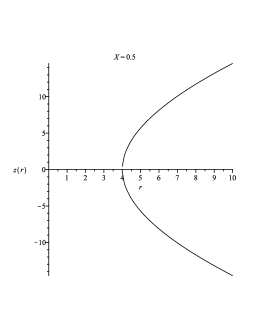
Fig. 1 : The profile curve of the wormhole.

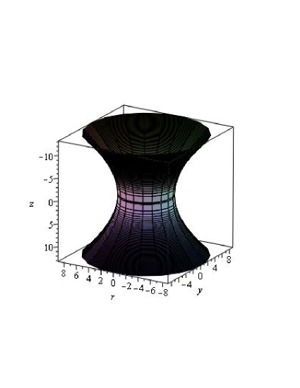
Fig. 2 : The embedding diagram generated by rotating the profile curve about the $z-$axis.

According to Morris and Thorne (1988), the $r$-coordinate is ill-behaved near the throat, but proper radial distance

$$l(r)=\pm\int_{r_{0}^{+}}^{r}\frac{dr}{\sqrt{1-\frac{b(r)}{r}}}$$ (39)

must be well behaved everywhere i.e. we must require that $l(r)$ is finite throughout the spacetime.

The proper radial distance $l(r)$ from the throat to a point outside is given in Fig. 3.

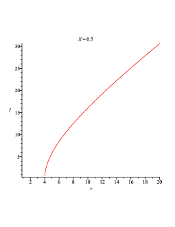
Fig. 3 : The graph of the radial proper distance $l(r)$

4.2 Energy Conditions

Now, we check the material compositions comprising the wormhole whether it will satisfy or not the null energy condition (NEC), weak energy condition (WEC) and strong energy condition (SEC) simultaneously at all points outside the source. Since we write all equations in terms of $X$ and follow the assumptions $A=0$ and $B=0$, we have

$$\rho^{eff}=\frac{X}{8\pi r_{0}^{2}}\left(\frac{r}{r_{0}}\right)^{X-3},$$ (40)

$$p_{r}^{eff}=-\frac{1}{8\pi r_{0}^{2}}\left(\frac{r}{r_{0}}\right)^{X-3},$$ (41)

$$p_{t}^{eff}=\frac{(1-X)}{16\pi r_{0}^{2}}\left(\frac{r}{r_{0}}\right)^{X-3},$$ (42)

$$\rho^{eff}+p_{r}^{eff}=\frac{(X-1)}{8\pi r_{0}^{2}}\left(\frac{r}{r_{0}}\right)^{X-3},$$ (43)

$$\rho^{eff}+p_{t}^{eff}=\frac{(1+X)}{16\pi r_{0}^{2}}\left(\frac{r}{r_{0}}\right)^{X-3},$$ (44)

$$\rho^{eff}+p_{r}^{eff}+2p_{t}^{eff}=0.$$ (45)

The Fig. 4 indicates that the null energy condition (NEC), weak energy condition (WEC) are violated, however, the strong energy condition (SEC) is satisfied marginally. Hence, in our models, the null energy condition (NEC) is violated to hold a wormhole open.

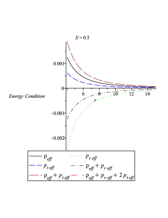
Fig. 4 : The variation of left hand side of the expressions of energy conditions are shown against $r$.

4.3 Equilibrium condition

Following Ponce de León Ponce de León (1993), we write the TOV Eq. (11) for an anisotropic fluid distribution, in the following form

$$-\frac{M_{G}\left(\rho^{eff}+p_{r}^{eff}\right)}{r^{2}}e^{\frac{\lambda-\nu}{2}}-\frac{dp_{r}^{eff}}{dr}+\frac{2}{r}\left(p_{t}^{eff}-p_{r}^{eff}\right)=0,$$ (46)

where $M_{G}=M_{G}(r)$ is the effective gravitational mass within the radius $r$ and is given by

$$M_{G}(r)=\frac{1}{2}r^{2}e^{\frac{\nu-\lambda}{2}}\nu^{\prime},$$ (47)

which can easily be derived from the Tolman-Whittaker formula and the Einstein’s field equations. Obviously, the modified TOV equation (46) describes the equilibrium condition for the wormhole subject to gravitational ($F_{g}$) and hydrostatic ($F_{h}$) plus another force due to the anisotropic nature ($F_{a}$) of the matter comprising the wormhole. Therefore, for equilibrium the above Eq. (46) can be written as

$$F_{g}+F_{h}+F_{a}=0,$$ (48)

where,

$$F_{g}=-\frac{\nu^{\prime}}{2}\left(\rho^{eff}+p_{r}^{eff}\right)=0,$$ (49)

$$F_{h}=-\frac{dp_{r}^{eff}}{dr}=\frac{(X-3)}{8\pi r_{0}^{3}}\left(\frac{r}{r_{0}}\right)^{X-4},$$ (50)

$$F_{a}=\frac{2}{r}\left(p_{t}^{eff}-p_{r}^{eff}\right)\\ =\frac{(3-X)}{8\pi r_{0}^{3}}\left(\frac{r}{r_{0}}\right)^{X-4}.$$ (51)

The profiles of $F_{g}$, $F_{h}$ and $F_{a}$ for our chosen source are shown in Fig. 5. The figure indicates that equilibrium stage can be achieved due to the combined effect of pressure anisotropic, gravitational and hydrostatic forces. It is to be distinctly noted that by virtue of the Eq. (30), the gravitational force term in Eq. (49) vanishes which is readily observed from the Fig. 5 as the plot for $F_{g}$ coincides with the coordinate $r$. The other two plots reside opposite to each other to make the system balanced.

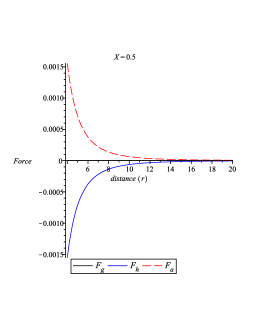
Fig. 5 : Three different forces acting on fluid elements in static equilibrium is shown against $r$.

4.4 Effective gravitational mass

In our model the effective gravitational mass, in terms of the effective energy density $\rho^{eff}$, can be expressed as

$$M^{eff}=4\pi\int_{r_{0}}^{R}\left(\rho+\rho^{de}\right)r^{2}dr$$

$$=4\pi\int_{r_{0}}^{R}\left[\frac{X}{8\pi r_{0}^{2}}\left(\frac{r}{r_{0}}\right)^{X-3}\right]r^{2}dr=\frac{R^{X}-r_{0}^{X}}{2r_{0}^{X-1}}.$$ (52)

The effective mass of the wormhole up to radius $8$ km from the throat (assuming the throat radius $r_{0}=4$ km and X=0.5) is obtained as $M^{eff}=.828~{}km=0.561~{}M_{\odot}$ (where $1$ Solar Mass $=1.475$ km).

We note from the Eq. (52) that though wormholes are supported by the exotic matter, but the effective mass is positive. This implies that for an observer sitting at large distance could not distinguish the gravitational nature between wormhole and a compact mass $M$.

4.5 Total gravitational energy

It is known that total gravitational energy of a localized real matter obeying all energy conditions is negative. Naturally, we would like to know how the gravitational energy behaves for the matters that supply fuel of our wormhole structure. Following Lynden-Bell et al. (2007) and Nandi et al. (2009), we have the following expression for the total gravitational energy of the wormhole as

$$E_{g}=\frac{1}{2}\int_{r_{0}}^{r}[~{}1-\sqrt{g_{rr}}~{}]\rho^{eff}r^{2}dr+\frac{r_{0}}{2},$$ (53)

where the second part is the contribution from the effective gravitational mass. It is to note that here the range of the integration is considered from the throat $r_{0}$ to the embedded radial space of the wormhole geometry. Here, the total gravitational energy of the wormhole is given by

$$E_{g}=\int_{r_{0}}^{r=ar_{0}}\left(\frac{X}{16\pi}\right)\left[1-\sqrt{\frac{1}{1-\left(\frac{r}{r_{0}}\right)^{X-1}}}\right]\left(\frac{r}{r_{0}}\right)^{X-1}dr$$

$$+\frac{r_{0}}{2}.$$ (54)

For the specific value of X, say $X=0.5$, we calculate the numerical value of the integrand (56) describing the total gravitational energy from the throat $r_{0}=4$ to the embedded radial space $1.5r_{0}=7$ (i.e. $a=1.5$) as $E_{g}=1.9397$, which indicates that $E_{g}>0$, in other words, there is a repulsion around the throat. This result is very much expected for constructing a physically valid wormhole. It is to be noted that the non-vanishing of $E_{G}$ explains why the wormhole is able to affect on the test particles despite $g_{tt}$ = constant (Nandi et al., 2009).

4.6 Traversability conditions

If the tidal gravitational forces felt by a traveler be reasonably small, then travel through wormhole is possible. Due to Morris et al. (1988), the acceleration experienced by the traveler should be less than the Earth’s gravity. A traveler of two meter height feels the tidal accelerations between two parts of his body should be less than the gravitational acceleration at Earth’s surface $g_{earth}$ ($g_{earth}\approx 10m/sec^{2}$). Now, the testing tangential tidal constraint is given by (assuming $\nu^{\prime}=0$)

$$|R_{t\theta t\theta}|=R_{t\phi t\phi}|=|\frac{\beta^{2}}{2r^{2}}(\frac{v}{c})^{2}(b^{\prime}-\frac{b}{r})|\leq\frac{g_{earth}}{2c^{2}m}$$

$$\approx\frac{1}{10^{10}m^{2}}$$ (55)

with $\beta=\frac{1}{\sqrt{1-(\frac{v}{c})^{2}}}$ and c is the velocity of light.

For $v<<c$, we have $\beta\approx 1$. We substitute the expression of our shape function to yield a restriction for the velocity as

$$\frac{v}{c}<\frac{1}{10^{8}}\frac{2r_{0}}{\sqrt{(1-X)(\frac{r}{r_{0}})^{X-2}}}$$ (56)

The above inequality represents the tangential tidal force and restrict the speed v of the while crossing the wormhole. Here radial acceleration is zero since $R_{rtrt}=0$, for our wormhole spacetime. Acceleration felt by a traveler should less than the gravitational acceleration at earth surface, $g_{earth}$. The condition imposed by Morris et al. (1988) is as follows:

$$|\textbf{f}|=|\sqrt{[1-\frac{b(r)}{r}}]\beta^{\prime}c^{2}|\leq g_{earth}~{}~{}for~{}~{}\nu^{\prime}~{}=~{}0.$$ (57)

For the traveler’s velocity $v=constant$, one finds that $|\textbf{f}|=0$. In our model the the above condition is automatically satisfied, the traveler feels a zero gravitational acceleration.

5 Final Remarks

In searching for a possibility of Lorentzian traversable wormhole in general relativity we have, in the present paper, considered the anisotropic dark energy along with the real matter source. The novel point here seems to be the interpretation in terms of two fluids, which is more or less arbitrary. We have constructed the wormholes from three different points of view (namely, specific shape function, specific energy density and constant redshift function) for the two non interacting fluids. To get realistic models, one has to impose different restrictions on the parameters. Fortunately, after imposing the restriction all the three models give the same structure of the wormhole.

Our main observations of the present investigation are as follows:

(1) The exotic matter though as usual violates null and weak energy conditions but does obey strong energy condition marginally.

(2) Since, $E_{g}>0$, there is a repulsion around the throat which is very much expected for valid construction of a wormhole.

Some of the other minor observations are as follows:

(1) For the spacetime to be asymptotically flat we note that, $\frac{b(r)}{r}~{}\longrightarrow 0$ as $r\longrightarrow\infty$ implies $X<1$. Flare-out condition, $b^{\prime}(r_{0})<1$ also gives, $X<1$.

(2) To travel through a wormhole, the tidal gravitational forces experienced by a traveler must be reasonably small. In our model the the above condition is automatically satisfied, the traveler feels a zero gravitational acceleration since $\nu=0$.

Based on the above observations we would like to conclude that the wormhole model provided here with anisotropic dark energy and real matter is fascinating in several aspects and hence very promising one.

However, we observe in the present investigation that anisotropic dark energy with different energy density and radial pressure may also provide the exotic fuel in constructing the wormhole. So, interpretations within dark energy or other than dark energy is needed for exotic sector of the energy-momentum tensor which can be sought for in a future work.

References

- Appleby et al. (2011) Appleby, S., Battye, R., Moss, A.: Int. J. Mod. Phys. D 20, 1153 (2011)
- Battye and Moss (2009) Battye, R., Moss, A.: Phys. Rev. D 80, 023531 (2009)
- Blome and Priester (1984) Blome, J.J., Priester, W.: Naturwiss. 71, 528 (1984)
- Bronnikov (1973) Bronnikov, K.: Acta Phys. Pol. B 4, 251 (1973)
- Buchdahl (1966) Buchdahl, H.A.: Astrophys. J. 160, 1512 (1966)
- Campanelli et al. (2010) Campanelli, L., Cea, P., Fogli, G.L., Tedesco, L.: Phys. Rev. D 81, 081301 (2010)
- Clement (1984) Clement, G.: Gen. Relativ. Gravit. 16, 477 (1984)
- Coleman and Korte (1985) Coleman, R.A., Korte, H.: in Hermann Weyl’s Raum - Zeit - Materie and a General Introduction to His Scientific Work, p. 199 (1985)
- Das and Kar (2005) Das, A., Kar, S.: Class. Quant. Gravit. 22, 3045 (2005)
- Davies (1984) Davies, P.C.W.: Phys. Rev. D 30, 737 (1984)
- Ellis (1973) Ellis, H.: J. Math. Phys. 14, 104 (1973)
- Freeman and McNamara (2006) Freeman, K., McNamara, G.: What can the matter be? In Search of Dark Matter, Birkhäuser Verlag, p. 105 (2006)
- Gribbin (2007) Gribbin, J.: The Origins of the Future: Ten Questions for the Next Ten Years, Yale University Press, p. 151 (2007)
- Hogan (1984) Hogan, C.: Nat. 310, 365 (1984)
- Jamil et al. (2010) Jamil, M., et al.: Eur. Phys. J. C 67, 513 (2010)
- Kaiser and Stebbins (1984) Kaiser, N., Stebbins, A.: Nat. 310, 391 (1984)
- Kuhfittig (1999) Kuhfittig, P.: Am. J. Phys. 67, 125 (1999)
- Kuhfittig et al. (2010) Kuhfittig, P., et al.: Int. J. Theor. Phys. 49, 1222 (2010)
- Landau and Lifshitz (1959) Landau, L.D., Lifshitz, E.M.: Fluid mechanics. Course of theoretical physics, Pergamon Press, Oxford (1959)
- Lobo (2005) Lobo, F.: Phys. Rev. D 71, 084011 (2005)
- Lobo (2006) Lobo, F.: Phys. Rev. D 73, 064028 (2006)
- Lynden-Bell et al. (2007) Lynden-Bell, D., Katz, J., Bic ak J: Phys. Rev. D 75, 024040 (2007)
- Morris et al. (1988) Morris, M.S., Thorne, K., Yurtsever,U.: Phys. Rev. Lett. 61, 1446 (1988)
- Morris and Thorne (1988) Morris, M.S., Thorne, K.S.: Am. J. Phys. 56, 395 (1988)
- Nandi et al. (2009) Nandi, K.K., Zhang, Y.Z., Cai, R.G., Panchenko, A.: Phys. Rev. D 79, 024011 (2009)
- Overduin and Cooperstock (1998) Overduin, J.M., Cooperstock, F.I.: Phys. Rev. D 58, 043506 (1998)
- Perlmutter et al. (1998) Perlmutter, S., et al.: Nat. 391, 51 (1998)
- Ponce de León (1993) Ponce de León, J.: Gen. Relativ. Gravit. 25, 1123 (1993)
- Pretzl (2004) Pretzl, K. Dark Matter, Massive Neutrinos and Susy Particles: Structure and Dynamics of Elementary Matter, Walter Greiner, p. 289 (2004)
- Rahaman et al. (2006) Rahaman, F., et al.: Phys. Lett. B 633, 161 (2006)
- Rahaman et al. (2007) Rahaman, F., et al.: Phys. Scr. 76, 56 (2007)
- Rahaman et al. (2008) Rahaman, F., et al.: Mod. Phys. Lett. A 23, 1199 (2008)
- Rahaman et al. (2009a) Rahaman, F., et al.: Acta Phys. Polon. B 40, 25 (2009)
- Rahaman et al. (2009b) Rahaman, F., et al.: Int. J. Theor. Phys. 48, 471 (2009)
- Rahaman et al. (2012) Rahaman, F., et al.: Gen. Relativ. Gravit. 44, 107 (2012)
- Riess et al. (1998) Riess, A.G., et al.: Astron. J. 116, 1009 (1998)
- Sahni and Starobinsky (2000) Sahni, V., Starobinsky, A.: Int. J. Mod. Phys. D 9, 373 (2000)
- Sushkov (2005) Sushkov, S.: Phys. Rev. D 71, 043520 (2005)
- Usmani et al. (2010) Usmani, A.A., et al.: Gen. Relativ. Gravit. 42, 2901 (2010)
- Visser (1989) Visser, M.: Phys. Rev. D 39, 3182 (1989)
- Visser (1996) Visser, M.: Lorentzian wormholes: From Einstein to Hawking, Springer (1996)
- Wheeler (1957) Wheeler, J.A.: Annals of Physics 2, 525 (1957)
- Wheeler (2007) Wheeler, J.C.: Cosmic Catastrophes: Exploding Stars, Black Holes, and Mapping the Universe, Cambridge University Press, p. 282 (2007)
- Zaslavskii (2005) Zaslavskii, O.: Phys. Rev. D 72, 061303 (2005)