The early stages of a high energy heavy ion collision

Abstract

At high energy, the gluon distribution in nuclei reaches large densities and eventually saturates due to recombinations, which plays an important role in heavy ion collisions at RHIC and the LHC. The Color Glass Condensate provides a framework for resumming these effects in the calculation of observables. In this talk, I present its application to the description of the early stages of heavy ion collisions.

1 Heavy ion collisions and color glass condensate

Because of the asymptotic freedom of strong interactions, the quark gluon plasma is the expected state of nuclear matter at sufficiently high temperature (above $T\sim 170$ MeV). Therefore, the early universe was presumably made of free quarks and gluons at times shorter than $\tau\sim 10^{-5}$ seconds (figure 1, left). Unfortunately, it seems that the confinement transition is too weak to have left any imprint that could be observable nowadays via astronomical observations, and we must therefore seek ways to study this state of nuclear matter in the laboratory.

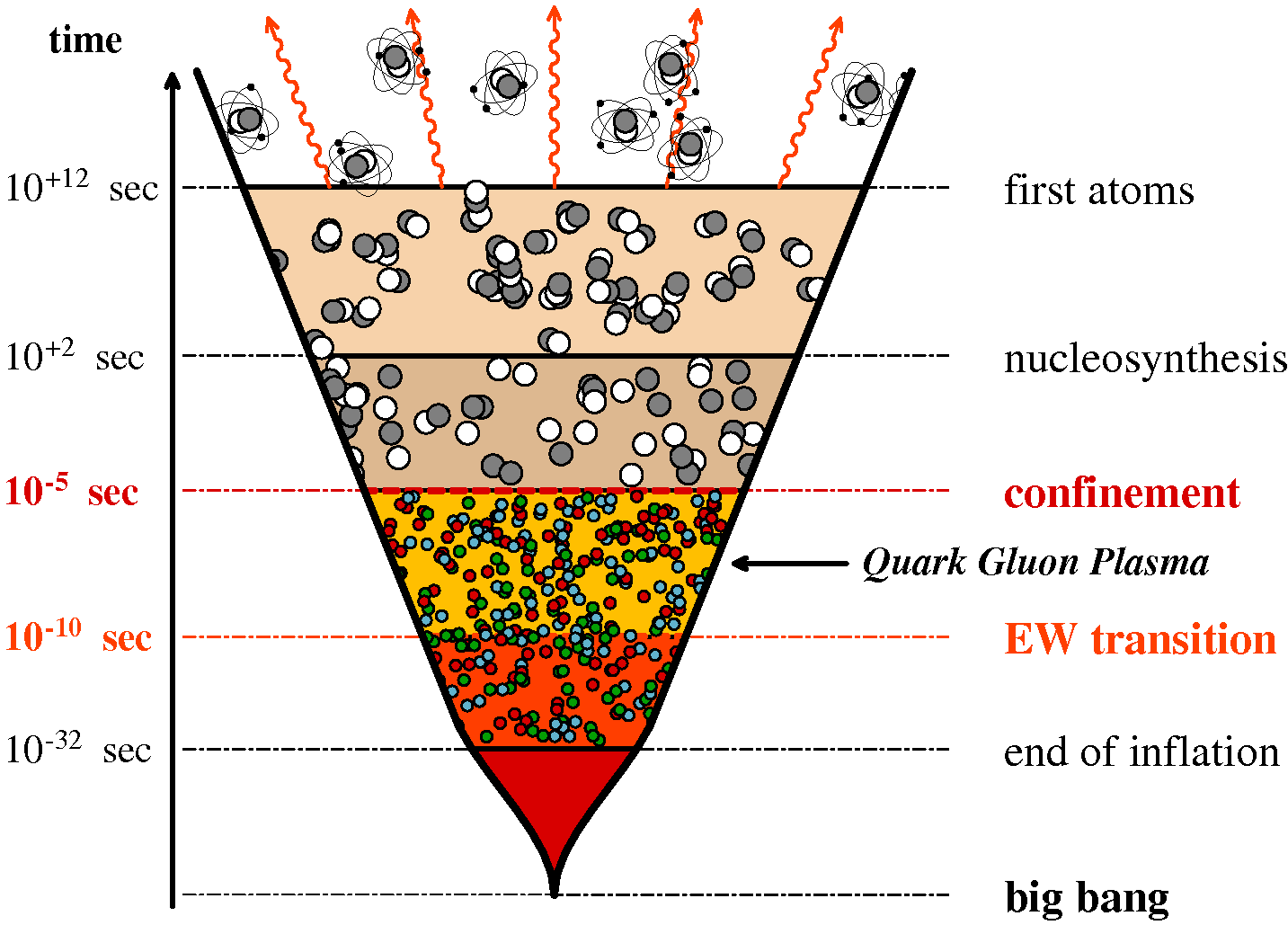
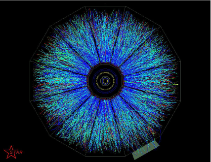
Figure 1: Left: the quark gluon plasma in the early universe. Right: event display of a heavy ion collision at RHIC (STAR collaboration).

It is expected that the conditions of this transition can be reached in collisions of large nuclei at ultra-relativistic energies. Such experiments are ongoing at RHIC (Brookhaven, USA) and at the the LHC (CERN), respectively at a maximum center of mass energy of $200$ GeV and $2.76~{}$TeV per nucleon pair (see the figure 1, right). There is ample evidence that the energy density reached in these collisions is (for a brief period of time) far above the critical energy density, and that deconfined quark-gluon matter is produced.

From a theoretical perspective, the evolution of the matter produced in the collision can be divided in several stages, that are handled by different tools (figure 2, left).

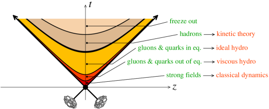
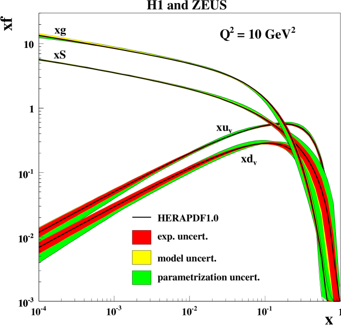
Figure 2: Left: stages of a heavy ion collision. Right: proton parton distributions (from [1]).

Broadly speaking, there are three main stages: (i) the collision itself, and a brief period of time afterwards, (ii) a longer stage where the matter is close to local thermal equilibrium, and (iii) the final stage during which the matter has become too dilute to remain in equilibrium. The focus of this talk is on the first of these three stages. During the time evolution, the matter produced in the collision expands, and therefore cools down. Therefore, this first stage is also characterized by the highest momentum scales which, by virtue of asymptotic freedom, suggests that one could describe it by a weak coupling expansion in Quantum Chromo-Dynamics (QCD). Unfortunately, the simplicity of the QCD Lagrangian,

$${\cal L}=-\frac{1}{4}{F^{2}}+\sum_{\rm flavors}{\overline{\psi}_{f}}(i{\raise 0.6458pt\hbox{$/$}\kern-5.29999pt\hbox{$D$}}-{m_{f}}){\psi_{f}}\;,$$ (1)

is deceptive and the situation is complicated by the very large gluon density in a nucleus at the relevant scales. In heavy ion collisions, the partons that play a role in the production of the bulk of the final state carry a very small fraction $x$ of the momentum of their parent nucleon, $x\sim P_{\perp}/\sqrt{s}$ (where $P_{\perp}$ is the transverse momentum of a typical final state particle and $\sqrt{s}$ the center of mass energy per nucleon pair.) This value ranges from $x\sim 10^{-2}$ (at RHIC) to $x\sim 10^{-4}$ (at the LHC). Measurements of the parton distributions in a proton (at HERA for instance, see the right panel of the figure 2) show that at such low values of $x$, the nucleon content is predominantly made of gluons, that have a very large density. This increase of the gluon density at low $x$ is due to the large emission probability of soft gluons (the differential probability behaves like $dP\sim\alpha_{s}dx/x$, where $\alpha_{s}$ is the coupling constant of strong interactions). However, this increase cannot continue forever: indeed, when the gluon occupation number becomes of the order of the inverse coupling $\alpha_{s}^{-1}$, the reverse process has a high probability – two gluons can then recombine, leading to a saturation of the gluon density [2]. This non-linear saturation mechanism generates a dynamical momentum scale –the saturation momentum, denoted $Q_{s}$–, below which saturation effects are important. This scale increases at small momentum fraction $x$ and increases with the mass number $A$ of a nucleus, as shown in the left panel of the figure 4. This is why saturation is expected to play a more important role in heavy ion collisions than in proton-proton collisions, even more so at the energy of the LHC.

Gluon densities of order $\alpha_{s}^{-1}$ lead to a breakdown of the plain perturbative expansion, making the saturation regime non-perturbative. For instance, Feynman graphs such as the one on the right of the figure 3 are as large as the one on the left.

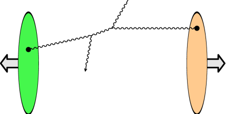
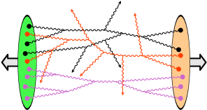
Figure 3: Left: collision of two dilute projectiles. Right: collision of two densely occupied projectiles.

The resummation of the infinite series of relevant graphs would be extremely cumbersome if attacked via standard Feynman rules. The Color Glass Condensate (CGC) [3] is an effective theory based on QCD that reorganizes the perturbative expansion in order to simplify this resummation. It does so by neglecting the quarks and by treating the fast partons (those at large $x$) as static color sources $J$ moving along the trajectories of the two projectiles, via the following effective Lagrangian

$${\cal S}=\underbrace{-\frac{1}{4}\int F_{\mu\nu}F^{\mu\nu}}_{{\cal S}_{{}_{\rm YM}}}+\int\underbrace{\vphantom{\int}({J^{\mu}_{1}+J^{\mu}_{2}})}_{\mbox{fast partons}}{A_{\mu}}\;.$$ (2)

In the saturated regime, these sources $J_{1,2}$ are large and must be resummed to all orders. One can write an expansion in powers of the coupling for observables, e.g.

$$\frac{dN_{1}}{dyd^{2}\vec{\boldsymbol{p}}_{\perp}}\sim{\frac{1}{\alpha_{s}}}\;\Big{[}c_{0}+c_{1}\,{\alpha_{s}}+c_{2}\,{\alpha_{s}^{2}}+\cdots\Big{]}$$ (3)

for the single inclusive gluon spectrum, but the coefficients $c_{i}$ in this expansion are non-perturbative functions of $J$. However, the advantage of this formulation is that quantum fields driven by a large source behave classically in a first approximation. This implies that at Leading Order in $\alpha_{s}$, observables can be obtained by solving the classical Yang-Mills equations [4],

$$\big{[}{{\cal D}_{\mu}},{{\cal F}^{\mu\nu}}\big{]}={J_{1}^{\nu}}+{J_{2}^{\nu}}\quad,\quad\lim_{t\to-\infty}{{\cal A}^{\mu}(t,\vec{\boldsymbol{x}})}=0\;,$$ (4)

instead of computing an infinite series of Feynman graphs.

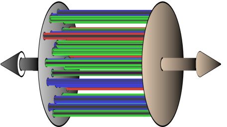
Figure 4: Left: saturation momentum as a function of $x$ and mass number $A$ (from [5]). Right: color flux tubes.

It turns out that this classical solution has a very peculiar feature, imposed by the geometry of the collision: at a proper time $\tau=0^{+}$, the lines of the chromo-electric and chromo-magnetic fields are all parallel to the collision axis [6] (see the figure 4, right). These fields form color flux tubes in the $z$ direction, that have a typical transverse size of order $Q_{s}^{-1}$. And the energy-momentum tensor of such a configuration of color fields is no less peculiar, since its longitudinal pressure is negative. Thus, this matter is initially very far from local thermodynamical equilibrium, and it is in fact a long standing puzzle to understand how (and if) it evolves towards thermalization.

2 Initial state factorization

Before we turn to the question of thermalization, let us first discuss another important issue: how do we know what sources $J_{1,2}$ we should use in the CGC approach to heavy ion collisions? The short answer is that for a given collision, we don’t. $J$ reflects the configuration (color and position in the transverse plane) of the fast partons of a nucleus at the time it collides with the second nucleus, and therefore the best we can hope for is to know the probability of having a certain configuration. Thus, the original question translates into: how do we know this distribution? It is possible to constrain this distribution by measurements done in other experiments, such as Deep Inelastic Scattering (DIS) on nuclei, provided one justifies its universality (i.e. that the distribution is the same for all inclusive observables in all experiments). In the case of DIS, it is know that the relevant distribution obeys the JIMWLK equation, that controls its evolution with energy.

In order to check whether the same is true in heavy ion collisions, one needs to consider higher order corrections to inclusive observables. These corrections contain logarithms of the collision energy, and one should check that these logarithms are the same as in DIS. At NLO, the single inclusive gluon spectrum can be written in the following way [7],

$$\left.{\frac{dN_{1}}{dyd^{2}\vec{\boldsymbol{p}}_{\perp}}}\right|_{{}_{\rm NLO}}=\Bigg{[}\frac{1}{2}\int\limits_{{}_{\vec{\boldsymbol{u}},\vec{\boldsymbol{v}}\in\Sigma}}{{\cal G}(\vec{\boldsymbol{u}},\vec{\boldsymbol{v}})}\,{\mathbbm{T}}_{\boldsymbol{u}}{\mathbbm{T}}_{\boldsymbol{v}}+\int\limits_{{}_{\vec{\boldsymbol{u}}\in\Sigma}}{{\boldsymbol{\beta}}(\vec{\boldsymbol{u}})}\,{\mathbbm{T}}_{\boldsymbol{u}}\Bigg{]}\;\left.{\frac{dN_{1}}{dyd^{2}\vec{\boldsymbol{p}}_{\perp}}}\right|_{{}_{\rm LO}}\;.$$ (5)

In this equation that relates the spectrum at LO and NLO, ${\mathbbm{T}}_{\boldsymbol{u}}$ is a functional derivative with respect to the classical field, and the functions ${\cal G}$ and $\beta$ can in principle be evaluated analytically ($\Sigma$ is a space-like surface used to set the initial condition for the classical field). The next step to justify the universality of the logarithms of energy is to prove that [7]

$$\frac{1}{2}\int\limits_{{}_{\vec{\boldsymbol{u}},\vec{\boldsymbol{v}}\in\Sigma}}{{\cal G}(\vec{\boldsymbol{u}},\vec{\boldsymbol{v}})}\,{\mathbbm{T}}_{\boldsymbol{u}}{\mathbbm{T}}_{\boldsymbol{v}}+\int\limits_{{}_{\vec{\boldsymbol{u}}\in\Sigma}}{{\boldsymbol{\beta}}(\vec{\boldsymbol{u}})}\,{\mathbbm{T}}_{\boldsymbol{u}}=\log\left(\Lambda^{+}\right)\,{{\cal H}_{1}}+\log\left(\Lambda^{-}\right)\,{{\cal H}_{2}}+\mbox{terms w/o logs}\;,$$ (6)

where ${\cal H}_{1,2}$ are the JIMWLK Hamiltonians of the two projectiles and $\Lambda^{\pm}$ the cutoffs that separate the fields from the fast sources in the CGC effective theory. A striking property of this formula is that the logarithms of $\Lambda^{+}$ (cutoff for the right-moving sources) and of $\Lambda^{-}$ (cutoff for the left-moving sources) do not mix: their coefficients are operators that depend only on $J_{1}$ or on $J_{2}$ respectively, but not both. It is this property that ensures that we can factorize these logarithms into distributions $W_{1}[J_{1}]$ and $W_{2}[J_{2}]$ that obey the JIMWLK equation,

$$\Lambda\frac{\partial W[J]}{\partial\Lambda}={\cal H}\,W[J]\;.$$ (7)

After averaging over these distributions of sources, the inclusive gluon spectrum at leading logarithmic accuracy reads

$$\left<\frac{dN_{1}}{dyd^{2}\vec{\boldsymbol{p}}_{\perp}}\right>_{{}_{\rm LLog}}=\int\big{[}D{J_{{}_{1}}}\,D{J_{{}_{2}}}\big{]}\;{W_{1}\big{[}J_{{}_{1}}\big{]}}\;{W_{2}\big{[}J_{{}_{2}}\big{]}}\;\underbrace{\frac{dN_{1}[J_{1,2}]}{dyd^{2}\vec{\boldsymbol{p}}_{\perp}}}_{\rm for\ fixed\ J_{1,2}}\Bigg{|}_{{}_{\rm LO}}\;.$$ (8)

It is this factorization formula that establishes a link between heavy ion collisions and DIS on a nucleus, since the same distribution $W[J]$ appears in both reactions.

The same reasoning can be applied to multi-gluon spectra, for which a similar factorization holds [8],

$$\left<\frac{dN_{n}}{dy_{1}d^{2}\vec{\boldsymbol{p}}_{1\perp}\cdots dy_{n}d^{2}\vec{\boldsymbol{p}}_{n\perp}}\right>_{{}_{\rm LLog}}\!\!=\int\big{[}D{J_{{}_{1}}}\,D{J_{{}_{2}}}\big{]}\;{W_{1}\big{[}J_{{}_{1}}\big{]}}\;{W_{2}\big{[}J_{{}_{2}}\big{]}}\;\frac{dN_{1}[J_{1,2}]}{dy_{1}d^{2}\vec{\boldsymbol{p}}_{1\perp}}\Bigg{|}_{{}_{\rm LO}}\!\!\!\!\cdots\frac{dN_{1}[J_{1,2}]}{dy_{n}d^{2}\vec{\boldsymbol{p}}_{n\perp}}\Bigg{|}_{{}_{\rm LO}}\!.$$ (9)

Since its integrand is fully factorized, this formula tells us that, at leading logarithmic accuracy, all the correlations between gluons separated in rapidity come from the evolution of the distributions $W[J]$ (in other words, these correlations are a property of the pre-collision initial state). On the basis of this formula, we expect long range correlations, over separations $\Delta y\sim\alpha_{s}^{-1}$ (since this is the change in rapidity that one needs in order to have an appreciable change in the distribution $W[J]$).

These rapidity correlations are particularly interesting experimentally in order to probe the early stages of heavy ion collisions, because a simple causality argument [9] (see the figure 5, left) indicates that long range rapidity correlations cannot be produced long after the collision.

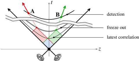
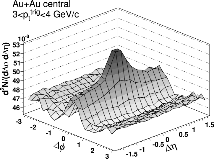
Figure 5: Left: causal connection between two particles at a large rapidity separation. Right: 2-hadron correlation in central heavy ion collisions (from [10]).

More precisely, if two particles are detected with a rapidity separation $\Delta y$, any process inducing a correlation between them must have taken place at a time $\tau$ smaller than $\tau_{\rm freeze\ out}\;e^{-|\Delta y|/2}$, which is a fairly stringent upper limit due to the exponential factor. As it turns out, such correlations have been observed in central heavy ion collisions (figure 5, right). These 2-hadron correlations extend quite far in rapidity [9], but are quite narrow in azimuthal angle. Note that the formula (9), while it predicts long range correlations in rapidity, does not lead to any appreciable collimation of the correlation in azimuthal angle. This is because it applies to the multi-gluon spectrum only at very short times after the collision. Subsequently, these gluons will be transported outwards by the hydrodynamical flow, and it is this radial flow that explains the azimuthal collimation seen experimentally [11].

3 Final state evolution and thermalization

When discussing the flux tube pattern that emerges at early times in the classical solution of the Yang-Mills equations, we mentioned in passing that this implies a negative longitudinal pressure. To be more definite, let us compare the energy-momentum tensor obtained at $\tau=0^{+}$ in the CGC framework at LO, with the tensor one would have in ideal hydrodynamics,

$${T^{\mu\nu}_{{}_{\rm CGC,LO}}(\tau=0^{+})=\begin{pmatrix}\epsilon&&&\\ &\epsilon&&\\ &&\epsilon&\\ &&&{-{\epsilon}}\\ \end{pmatrix}}\quad,\quad{T^{\mu\nu}_{\rm ideal\ hydro}=\begin{pmatrix}\epsilon&&&\\ &p&&\\ &&p&\\ &&&p\\ \end{pmatrix}}\;.$$ (10)

With viscous hydrodynamics, one may cope with a certain degree of asymmetry between the transverse and longitudinal pressures, but not to the extent required to accommodate a negative longitudinal pressure.

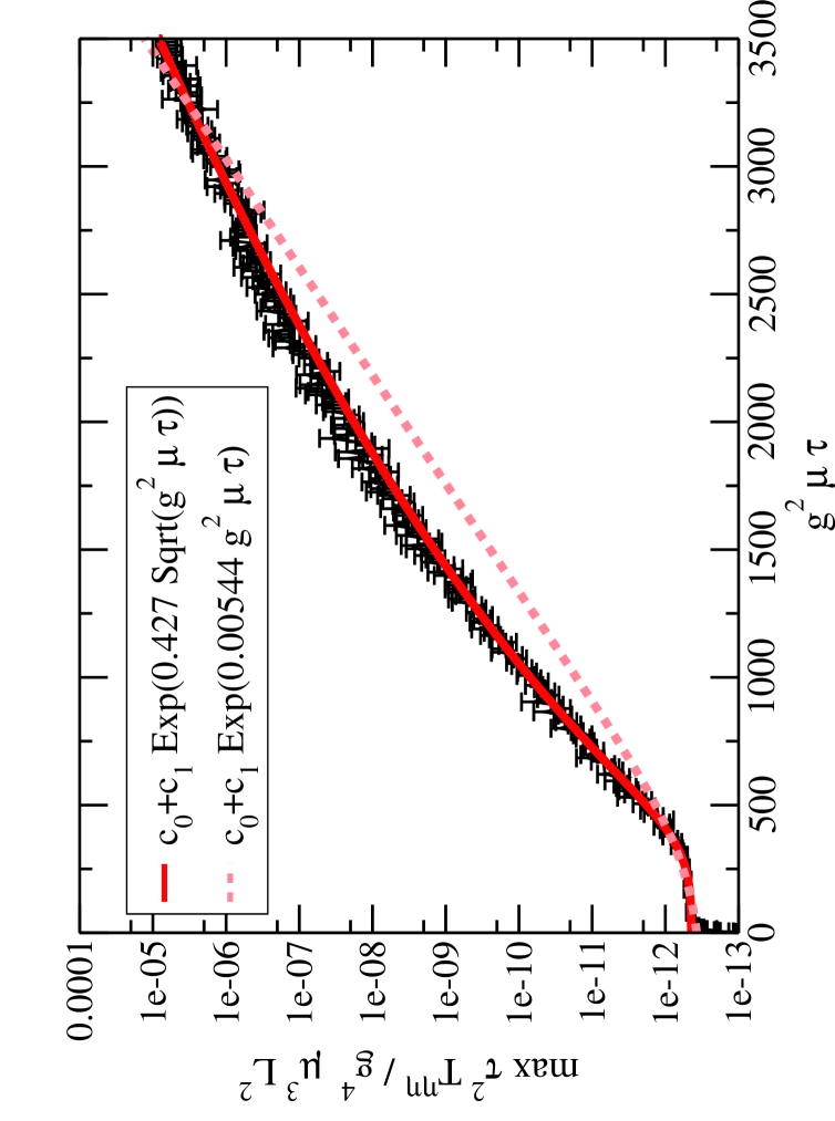
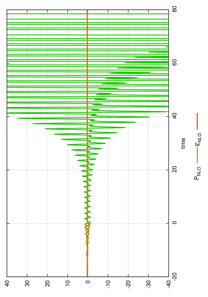
Figure 6: Left: instabilities in classical Yang-Mills equations (from [12]). Right: energy density and pressure at NLO in a toy scalar model.

However, it has also been known for a while that the LO result cannot be the final answer, due to the existence of instabilities in asymmetric systems of classical color fields [12, 13]. In the CGC, this issue appears in the form of unstable modes in the classical Yang-Mills equations: when the initial condition is perturbed by a rapidity dependent fluctuation, the solution may diverge exponentially from the unperturbed solution (see the figure 6, left). These unstable modes first appear in the energy-momentum tensor at NLO, where they lead to secular divergences in the pressure, and thus to a complete breakdown of the expansion in powers of $\alpha_{s}$. It would therefore be highly desirable to perform a resummation that cures these divergences.

In order to explore these ideas while avoiding most of the technical complications specific to a gauge theory, we have considered a much simpler $\phi^{4}$ scalar toy model that exhibits similar problems. It Lagrangian is given by

$${\cal L}=\frac{1}{2}(\partial_{\alpha}\phi)^{2}-V(\phi)+J\phi\quad,\qquad V(\phi)=\frac{g^{2}}{4!}\phi^{4}\;,\quad J\propto\theta(-x^{0})\;.$$ (11)

Like a Yang-Mills theory, this model is scale invariant in $3+1$ dimensions (i.e. the only dimensionful scale in our model is brought by the classical source $J$). In order to mimic a collision, we turn off the source at $x^{0}>0$ (thus, the sole purpose of the source is to initialize the classical fields at $x^{0}=0$). The reason why this model is a good playground to study the CGC instabilities is that it also has unstable modes due to parametric resonance. The dramatic effect of these instabilities is shown in the right panel of the figure 6, where one sees that the NLO correction to the pressure explodes exponentially with time.

In order to improve the late time behavior of the pressure, we need a resummation that restores the non-linearities in the unstable modes (these modes are linearized when one does an expansion in powers of $g^{2}$ at fixed order). A good starting point to find such a resummation is the formula that relates the LO and NLO:

$${T^{\mu\nu}_{{}_{\rm NLO}}}=\Bigg{[}\frac{1}{2}\int\limits_{{}_{\vec{\boldsymbol{u}},\vec{\boldsymbol{v}}\in\Sigma}}{{\cal G}(\vec{\boldsymbol{u}},\vec{\boldsymbol{v}})}\,{\mathbbm{T}}_{\boldsymbol{u}}{\mathbbm{T}}_{\boldsymbol{v}}+\int\limits_{{}_{\vec{\boldsymbol{u}}\in\Sigma}}{{\boldsymbol{\beta}}(\vec{\boldsymbol{u}})}\,{\mathbbm{T}}_{\boldsymbol{u}}\Bigg{]}\;{T^{\mu\nu}_{{}_{\rm LO}}}\;.$$ (12)

By exponentiating the operator in the square brackets,

$${T^{\mu\nu}_{{}_{\rm resummed}}}={\exp}\Bigg{[}\frac{1}{2}\int\limits_{{}_{\vec{\boldsymbol{u}},\vec{\boldsymbol{v}}\in\Sigma}}{{\cal G}(\vec{\boldsymbol{u}},\vec{\boldsymbol{v}})}\,{\mathbbm{T}}_{\boldsymbol{u}}{\mathbbm{T}}_{\boldsymbol{v}}+\int\limits_{{}_{\vec{\boldsymbol{u}}\in\Sigma}}{{\boldsymbol{\beta}}(\vec{\boldsymbol{u}})}\,{\mathbbm{T}}_{\boldsymbol{u}}\Bigg{]}\;{T^{\mu\nu}_{{}_{\rm LO}}}\;,$$ (13)

it is clear that one obtains in full the LO and NLO contributions, plus a subset of the higher order terms,

$$T^{\mu\nu}_{{}_{\rm resummed}}\sim{\frac{1}{g^{2}}}\;\Big{[}\underbrace{c_{0}+c_{1}\,{g^{2}}}_{\mbox{fully}}+\underbrace{c_{2}\,{g^{4}}+\cdots}_{\mbox{partly}}\Big{]}\;.$$ (14)

This exponentiation can be justified as the resummation that picks at each order in $g^{2}$ the fastest growing unstable terms. Let us now show that this resummation eliminates the secular divergence encountered at NLO, by noticing that

$${\exp}\Bigg{[}\frac{1}{2}\int\limits_{{}_{\vec{\boldsymbol{u}},\vec{\boldsymbol{v}}}}\!{{\cal G}(\vec{\boldsymbol{u}},\vec{\boldsymbol{v}})}\,{\mathbbm{T}}_{\boldsymbol{u}}{\mathbbm{T}}_{\boldsymbol{v}}+\int\limits_{{}_{\vec{\boldsymbol{u}}}}{{\boldsymbol{\beta}}(\vec{\boldsymbol{u}})}\,{\mathbbm{T}}_{\boldsymbol{u}}\Bigg{]}\,T^{\mu\nu}_{{}_{\rm LO}}[\varphi_{\rm init}]$$

$$=\int[D{\alpha}]\,\exp\Bigg{[}-\frac{1}{2}\int\limits_{{}_{\vec{\boldsymbol{u}},\vec{\boldsymbol{v}}}}\!{\cal G}^{{}^{-1}}\!(\vec{\boldsymbol{u}},\vec{\boldsymbol{v}}){\alpha(\vec{\boldsymbol{u}})}{\alpha(\vec{\boldsymbol{v}})}\Bigg{]}\,T^{\mu\nu}_{{}_{\rm LO}}[\varphi_{\rm init}+{\beta}+{\alpha}]\;.$$ (15)

In words, this resummation amounts to a Gaussian smearing of the initial classical field in the LO calculation. Since the LO result is free of any secular divergence, this resummed result is finite at all times as well. A similar resummation has in fact been proposed in other areas before, such as inflationary cosmology [14] and Bose-Einstein condensation [15]. This Gaussian ensemble of initial fields can also be interpreted as a pure quantum mechanical coherent state, because it has the minimal extension required by the uncertainty principle, shared evenly by the fields and their conjugate momenta.

The other virtue of this resummation is that it is fairly easy to implement numerically, in order to check what effect it has on the evolution of the energy-momentum tensor.

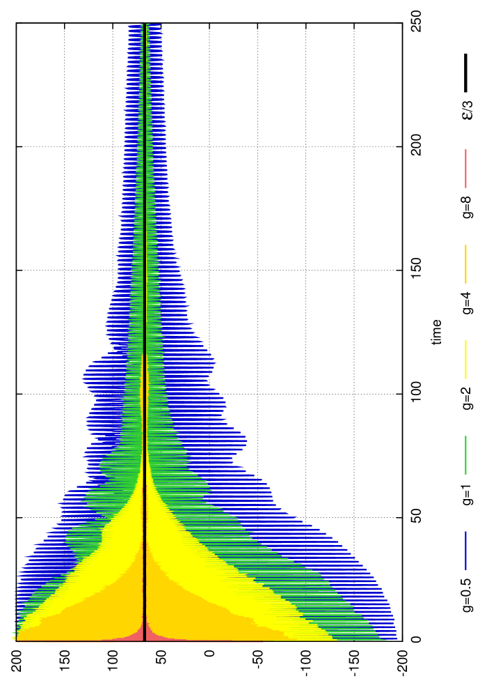
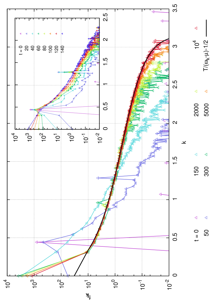
Figure 7: Left: energy density and pressure after resummation, for various values of the coupling $g$. Right: occupation number at various times.

This computation merely amounts to solving classical field equations of motion (the non-linear Klein-Gordon equation in the case of this scalar toy model) repeatedly with initial conditions drawn randomly from a Gaussian ensemble [16]. When this procedure is applied to the energy-momentum tensor, one finds a result which is very different from what we got in a strict NLO calculation (see the figure 7, left). Now, not only the pressure does not diverge at late times, but its oscillations are damped and eventually one has $p=\epsilon/3$, which is nothing but the equilibrium equation of state of a scale invariant system in three spatial dimensions. Note also that the relaxation time of the pressure decreases with increasing values of the coupling constant. In a simplified study where only the zero momentum fluctuations are included, it is possible to see analytically that the relaxation of the pressure is due to the loss of coherence of the initial wavefunction under the effect of nonlinear interactions. One can also compute the occupation number in this system and its time evolution (figure 7, right). One sees that it evolves to an equilibrium distribution, but on time-scales that are longer than those associated to decoherence. Interestingly, when the initial condition corresponds to a large energy density carried by soft modes, a Bose-Einstein condensate forms in the system, and survives for a very long time if the coupling is weak. Indeed, at weak coupling the inelastic interactions that could get rid of the excess of particles in the condensate are quite suppressed compared to the elastic processes that tend to populate the condensate. Although this study seems promising, it would be extremely interesting to see how much of these features survive in a longitudinally expanding system –as is the case in the geometry of a collision–, with gauge fields rather than scalar fields (see [17] for recent works).

I would like to thank the organizers of the Rutherford Centennial Conference on Nuclear Physics for their kind invitation, and my collaborators J.-P. Blaizot, K. Dusling, T. Epelbaum, K. Fukushima, T. Lappi, J. Liao, L. McLerran and R. Venugopalan.

References

References

- [1] F.D. Aaron, et al, [H1 and ZEUS Collaborations] JHEP 1001, 109 (2010).
- [2] L. Gribov, E. Levin, M. Ryskin, Phys. Rept. 100, 1 (1983).
- [3] E. Iancu, A. Leonidov, L.D. McLerran, Lectures given at Cargese Summer School on QCD Perspectives on Hot and Dense Matter, Cargese, France, 6-18 Aug 2001, hep-ph/0202270; E. Iancu, R. Venugopalan, Quark Gluon Plasma 3, Eds. R.C. Hwa and X.N. Wang, World Scientific, hep-ph/0303204; F. Gelis, E. Iancu, J. Jalilian-Marian, R. Venugopalan, Ann. Rev. Part. Nucl. Sci. 60, 463 (2010).
- [4] A. Krasnitz, R. Venugopalan, Phys. Rev. Lett. 86, 1717 (2001); A. Krasnitz, R. Venugopalan, Nucl. Phys. B 557, 237 (1999); T. Lappi, Phys. Rev. C 67, 054903 (2003).
- [5] A. Deshpande, R. Ent, R. Milner, CERN Courier, October 2009.
- [6] T. Lappi, L.D. McLerran, Nucl. Phys. A 772, 200 (2006).
- [7] F. Gelis, T. Lappi, R. Venugopalan, Phys. Rev. D 78, 054019 (2008).
- [8] F. Gelis, T. Lappi, R. Venugopalan, Phys. Rev. D 78, 054020 (2008); F. Gelis, T. Lappi, R. Venugopalan, Phys. Rev. D 79, 094017 (2009).
- [9] A. Dumitru, K. Dusling, F. Gelis, J. Jalilian-Marian, T. Lappi, R. Venugopalan, Phys. Lett. B 697, 21 (2011); K. Dusling, F. Gelis, T. Lappi, R. Venugopalan, Nucl. Phys. A 836, 159 (2010).
- [10] B.I. Abelev, et al., [STAR Collaboration] Phys. Rev. C 80, 064912 (2009).
- [11] S.A. Voloshin, Phys. Lett. B 632, 490 (2006); E.V. Shuryak, Phys. Rev. C 76, 047901 (2007).
- [12] P. Romatschke, R. Venugopalan, Phys. Rev. Lett. 96, 062302 (2006).
- [13] U.W. Heinz, C.R. Hu, S. Leupold, S.G. Matinyan, B. Muller, Phys. Rev. D 55, 2464 (1997); T. Kunihiro, B. Muller, A. Ohnishi, A. Schafer, T.T. Takahashi, A Yamamoto, Phys. Rev. D 82, 114015 (2010); P. Romatschke, R. Venugopalan, Phys. Rev. D 74, 045011 (2006); K. Fukushima, F. Gelis, arXiv:1106.1396.
- [14] D.T. Son, hep-ph/9601377; S.Yu. Khlebnikov, I.I. Tkachev, Phys. Rev. Lett. 77, 219 (1996).
- [15] A.A. Norrie, R.J. Ballagh, C.W. Gardiner, arXiv:cond-mat/0403378.
- [16] K. Dusling, T. Epelbaum, F. Gelis, R. Venugopalan, Nucl. Phys. A 850, 69 (2011); T. Epelbaum, F. Gelis, arXiv:1107.0668 [hep-ph], to appear in Nucl. Phys. A.
- [17] J.P. Blaizot, F. Gelis, J. Liao, L. McLerran, R. Venugopalan, arXiv:1107.5296; A. Kurkela, G.D. Moore, arXiv:1107.5050, arXiv:1108.4684.