Performance of the ATLAS Trigger System in 2010t1

Abstract

Proton-proton collisions at $\sqrt{s}={7}{\mathrm{\ Te\kern-1.00006ptV}}$ and heavy ion collisions at $\sqrt{s_{NN}}=2.76{\mathrm{\ Te\kern-1.00006ptV}}$ were produced by the LHC and recorded using the ATLAS experiment’s trigger system in 2010. The LHC is designed with a maximum bunch crossing rate of 40 MHz and the ATLAS trigger system is designed to record approximately 200 of these per second. The trigger system selects events by rapidly identifying signatures of muon, electron, photon, tau lepton, jet, and $B$ meson candidates, as well as using global event signatures, such as missing transverse energy. An overview of the ATLAS trigger system, the evolution of the system during 2010 and the performance of the trigger system components and selections based on the 2010 collision data are shown. A brief outline of plans for the trigger system in 2011 is presented.

1 Introduction

ATLAS DetectorPaper is one of two general-purpose experiments recording LHC LHCPaper collisions to study the Standard Model (SM) and search for physics beyond the SM. The LHC is designed to operate at a centre of mass energy of $\sqrt{s}={14}{\mathrm{\ Te\kern-1.00006ptV}}$ in proton-proton ($pp$) collision mode with an instantaneous luminosity $\mathcal{L}=10^{34}\,\text{cm}^{-2}\text{s}^{-1}$ and at $\sqrt{s_{NN}}=2.76{\mathrm{\ Te\kern-1.00006ptV}}$ in heavy-ion ($PbPb$) collision mode with $\mathcal{L}=10^{31}\,\text{cm}^{-2}\text{s}^{-1}$. The LHC started single-beam operation in 2008 and achieved first collisions in 2009. During a prolonged period of $pp$ collision operation in 2010 at $\sqrt{s}={7}{\mathrm{\ Te\kern-1.00006ptV}}$, ATLAS collected 45 pb^-1of data with luminosities ranging from $10^{27}\,\text{cm}^{-2}\text{s}^{-1}$ to $2\cdot 10^{32}\,\text{cm}^{-2}\text{s}^{-1}$. The $pp$ running was followed by a short period of heavy ion running at $\sqrt{s_{NN}}=2.76{\mathrm{\ Te\kern-1.00006ptV}}$  in which ATLAS collected 9.2 $\mu$b^-1of $PbPb$ collisions.

Focusing mainly on the $pp$ running, the performance of the ATLAS trigger system during 2010 LHC operation is presented in this paper. The ATLAS trigger system is designed to record events at approximately 200 Hz from the LHC’s 40 MHz bunch crossing rate. The system has three levels; the first level (L1) is a hardware-based system using information from the calorimeter and muon sub-detectors, the second (L2) and third (Event Filter, EF) levels are software-based systems using information from all sub-detectors. Together, L2 and EF are called the High Level Trigger (HLT).

For each bunch crossing, the trigger system verifies if at least one of hundreds of conditions (triggers) is satisfied. The triggers are based on identifying combinations of candidate physics objects (signatures) such as electrons, photons, muons, jets, jets with $b$-flavour tagging ($b$-jets) or specific $B$-physics decay modes. In addition, there are triggers for inelastic $pp$ collisions (minbias) and triggers based on global event properties such as missing transverse energy ($E_{\mathrm{T}}^{\mathrm{miss}}$) and summed transverse energy ($\sum E_{\text{T}}$).

In Section 2, following a brief introduction to the ATLAS detector, an overview of the ATLAS trigger system is given and the terminology used in the remainder of the paper is explained. Section 3 presents a description of the trigger system commissioning with cosmic rays, single-beams, and collisions. Section 4 provides a brief description of the L1 trigger system. Section 5 introduces the reconstruction algorithms used in the HLT to process information from the calorimeters, muon spectrometer, and inner detector tracking detectors. The performance of the trigger signatures, including rates and efficiencies, is described in Section 6. Section 7 describes the overall performance of the trigger system. The plans for the trigger system operation in 2011 are described in Section 8.

2 Overview

The ATLAS detector DetectorPaper shown in Fig. 1, has a cylindrical geometry which covers almost the entire solid angle around the nominal interaction point. Owing to its cylindrical geometry, detector components are described as being part of the barrel if they are in the central region of pseudo-rapidity or part of the end-caps if they are in the forward regions. The ATLAS detector is composed of the following sub-detectors:

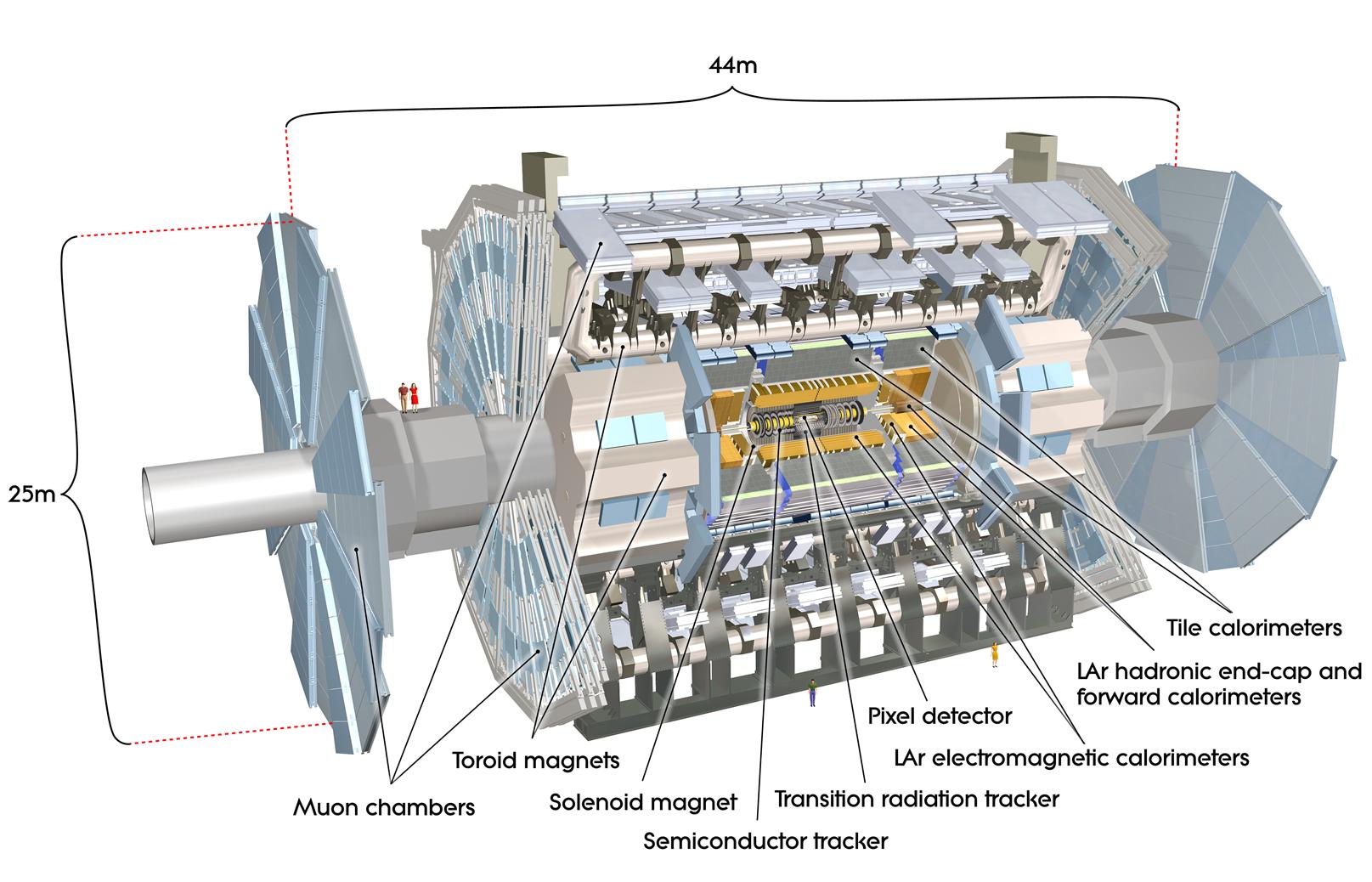
Figure 1: The ATLAS detector

•

Inner Detector: The Inner Detector tracker (ID) consists of a silicon pixel detector nearest the beam-pipe, surrounded by a SemiConductor Tracker (SCT) and a Transition Radiation Tracker (TRT). Both the Pixel and SCT cover the region $|\eta|<2.5$, while the TRT covers $|\eta|<2$. The ID is contained in a 2 Tesla solenoidal magnetic field. Although not used in the L1 trigger system, tracking information is a key ingredient of the HLT.

•

Calorimeter: The calorimeters cover the region $|\eta|<4.9$ and consist of electromagnetic (EM) and hadronic (HCAL) calorimeters. The EM, Hadronic End-Cap (HEC) and Forward Calorimeters (FCal) use a Liquid Argon and absorber technology (LAr). The central hadronic calorimeter is based on steel absorber interleaved with plastic scintillator (Tile). A presampler is installed in front of the EM calorimeter for $|\eta|<1.8$. There are two separate readout paths: one with coarse granularity (trigger towers) used by L1, and one with fine granularity used by the HLT and offline reconstruction.

•

Muon Spectrometer: The Muon Spectrometer (MS) detectors are mounted in and around air core toroids that generate an average field of 0.5 T in the barrel and 1 T in the end-cap regions. Precision tracking information is provided by Monitored Drift Tubes (MDT) over the region $|\eta|<2.7$ ($|\eta|<2.0$ for the innermost layer) and by Cathode Strip Chambers (CSC) in the region $2<|\eta|<2.7$. Information is provided to the L1 trigger system by the Resistive Plate Chambers (RPC) in the barrel ($|\eta|<1.05$) and the Thin Gap Chambers (TGC) in the end-caps ($1.05<|\eta|<2.4$).

•

Specialized detectors: Electrostatic beam pick-up devices (BPTX) are located at $z=\pm$175 m. The Beam Conditions Monitor (BCM) consists of two stations containing diamond sensors located at $z=\pm$1.84 m, corresponding to $|\eta|\simeq 4.2$. There are two forward detectors, the LUCID Cerenkov counter covering $5.4<|\eta|<5.9$ and the Zero Degree Calorimeter (ZDC) covering $|\eta|>8.3$. The Minimum Bias Trigger Scintillators (MBTS), consisting of two scintillator wheels with 32 counters mounted in front of the calorimeter end-caps, cover $2.1<|\eta|<3.8$.

When operating at the design luminosity of $10^{34}\,\text{cm}^{-2}\text{s}^{-1}$ the LHC will have a 40 MHz bunch crossing rate, with an average of 25 interactions per bunch crossing. The purpose of the trigger system is to reduce this input rate to an output rate of about 200 Hz for recording and offline processing. This limit, corresponding to an average data rate of $\sim$300 MB/s, is determined by the computing resources for offline storage and processing of the data. It is possible to record data at significantly higher rates for short periods of time. For example, during 2010 running there were physics benefits from running the trigger system with output rates of up to $\sim$600 Hz. During runs with instantaneous luminosity $\sim 10^{32}\,\text{cm}^{-2}\text{s}^{-1}$, the average event size was $\sim$1.3 MB.

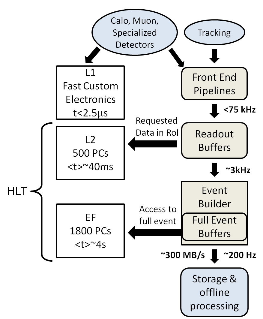
Figure 2: Schematic of the ATLAS trigger system

A schematic diagram of the ATLAS trigger system is shown in Fig. 2. Detector signals are stored in front-end pipelines pending a decision from the L1 trigger system. In order to achieve a latency of less than 2.5 $\mu$s, the L1 trigger system is implemented in fast custom electronics. The L1 trigger system is designed to reduce the rate to a maximum of 75 kHz. In 2010 running, the maximum L1 rate did not exceed 30 kHz. In addition to performing the first selection step, the L1 triggers identify Regions of Interest (RoIs) within the detector to be investigated by the HLT.

The HLT consists of farms of commodity processors connected by fast dedicated networks (Gigabit and 10 Gigabit Ethernet). During 2010 running, the HLT processing farm consisted of about 800 nodes configurable as either L2 or EF and 300 dedicated EF nodes. Each node consisted of eight processor cores, the majority with a 2.4 GHz clock speed. The system is designed to expand to about 500 L2 nodes and 1800 EF nodes for running at LHC design luminosity. When an event is accepted by the L1 trigger (referred to as an L1 accept), data from each detector are transferred to the detector-specific Readout Buffers (ROB) , which store the event in fragments pending the L2 decision. One or more ROBs are grouped into Readout Systems (ROS) which are connected to the HLT networks. The L2 selection is based on fast custom algorithms processing partial event data within the RoIs identified by L1. The L2 processors request data from the ROS corresponding to detector elements inside each RoI, reducing the amount of data to be transferred and processed in L2 to 2–6% of the total data volume. The L2 triggers reduce the rate to $\sim$3 kHz with an average processing time of $\sim$40 ms/event. Any event with an L2 processing time exceeding 5 s is recorded as a timeout event. During runs with instantaneous luminosity $\sim 10^{32}\,\text{cm}^{-2}\text{s}^{-1}$, the average processing time of L2 was $\sim$50 ms/event (Section 7).

The Event Builder assembles all event fragments from the ROBs for events accepted by L2, providing full event information to the EF. The EF is mostly based on offline algorithms invoked from custom interfaces for running in the trigger system. The EF is designed to reduce the rate to  $\sim$200 Hz with an average processing time of $\sim$4 s/event. Any event with an EF processing time exceeding 180 s is recorded as a timeout event. During runs with instantaneous luminosity $\sim 10^{32}\,\text{cm}^{-2}\text{s}^{-1}$, the average processing time of EF was $\sim$0.4 s/event (Section 7).

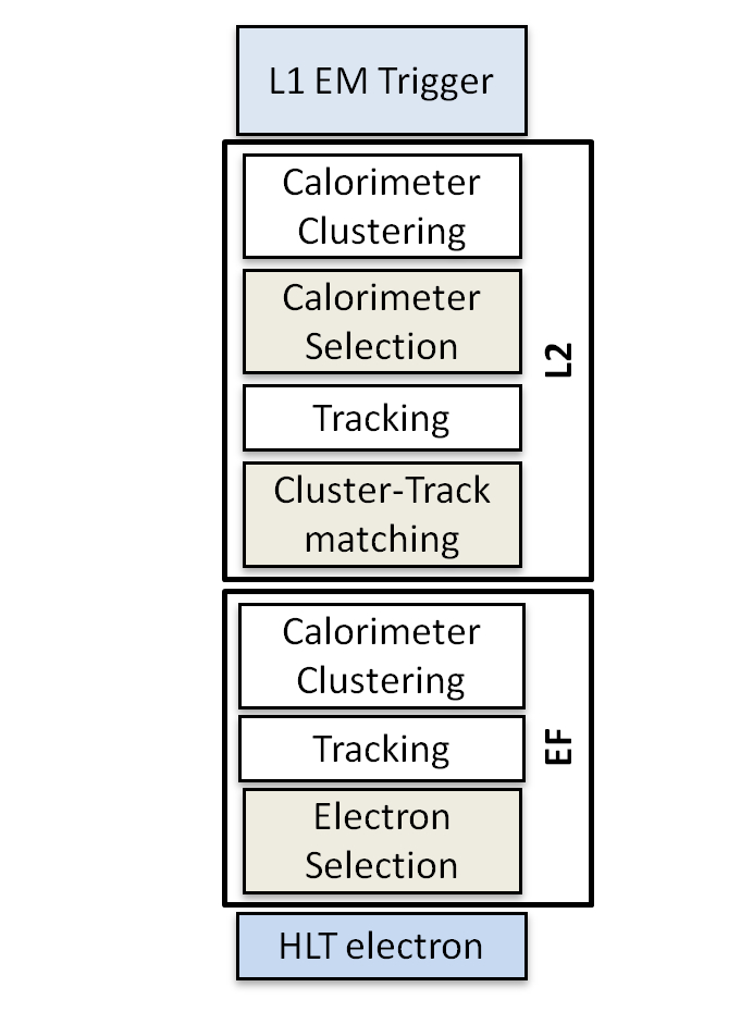
Figure 3: Electron trigger chain

Table 1: The key trigger objects, the shortened names used to represent them in the trigger menu at L1 and the HLT, and the L1 thresholds used for each trigger signature in the menu at $\mathcal{L}$=$10^{32}\,\text{cm}^{-2}\text{s}^{-1}$. Thresholds are applied to $E_{\mathrm{T}}$ for calorimeter triggers and $p_{\mathrm{T}}$ for muon triggers

	Representation
Trigger Signature	L1	HLT	L1 Thresholds [GeV]
electron	EM	e	2	3	5	10	10i	14	14i	85
photon	EM	g	2	3	5	10	10i	14	14i	85
muon	MU	mu	0	6	10	15	20
jet	J	j	5	10	15	30	55	75	95	115
forward jet	FJ	fj	10	30	55	95
tau	TAU	tau	5	6	6i	11	11i	20	30	50
$E_{\mathrm{T}}^{\mathrm{miss}}$	XE	xe	10	15	20	25	30	35	40	50
$\sum E_{\text{T}}$	TE	te	20	50	100	180
total jet energy	JE	je	60	100	140	200
$b$ jet	—	b
MBTS	MBTS	mbts
BCM	BCM	—
ZDC	ZDC	—
LUCID	LUCID	—
Beam Pickup (BPTX)	BPTX	—

Data for events selected by the trigger system are written to inclusive data streams based on the trigger type. There are four primary physics streams, Egamma, Muons, JetTauEtmiss, MinBias, plus several additional calibration streams. Overlaps and rates for these streams are shown in Section 7. About 10% of events are written to an express stream where prompt offline reconstruction provides calibration and Data Quality (DQ) information prior to the reconstruction of the physics streams. In addition to writing complete events to a stream, it is also possible to write partial information from one or more sub-detectors into a stream. Such events, used for detector calibration, are written to the calibration streams.

The trigger system is configured via a trigger menu which defines trigger chains that start from a L1 trigger and specify a sequence of reconstruction and selection steps for the specific trigger signatures required in the trigger chain. A trigger chain is often referred to simply as a trigger. Figure 3 shows an illustration of a trigger chain to select electrons. Each chain is composed of Feature Extraction (FEX) algorithms which create the objects (like calorimeter clusters) and Hypothesis (HYPO) algorithms that apply selection criteria to the objects (e.g. transverse momentum greater than 20 GeV). Caching in the trigger system allows features extracted from one chain to be re-used in another chain, reducing both the data access and processing time of the trigger system.

Approximately 500 triggers are defined in the current trigger menus. Table 1 shows the key physics objects identified by the trigger system and gives the shortened representation used in the trigger menus. Also shown are the L1 thresholds applied to transverse energy ($E_{\mathrm{T}}$) for calorimeter triggers and transverse momentum ($p_{\mathrm{T}}$) for muon triggers. The menu is composed of a number of different classes of trigger:

•

Single object triggers: used for final states with at least one characteristic object. For example, a single muon trigger with a nominal $6{\mathrm{\ Ge\kern-1.00006ptV}}$ threshold is referred to in the trigger menu as mu6.

•

Multiple object triggers: used for final states with two or more characteristic objects of the same type. For example, di-muon triggers for selecting $J/\psi\rightarrow\mathrm{\mu\mu}$ decays. Triggers requiring a multiplicity of two or more are indicated in the trigger menu by prepending the multiplicity to the trigger name, as in, 2mu6.

•

Combined triggers: used for final states with two or more characteristic objects of different types. For example, a $13{\mathrm{\ Ge\kern-1.00006ptV}}$ muon plus $20{\mathrm{\ Ge\kern-1.00006ptV}}$ missing transverse energy ($E_{\mathrm{T}}^{\mathrm{miss}}$) trigger for selecting $W\rightarrow\mu\nu$ decays would be denoted mu13_xe20.

•

Topological triggers: used for final states that require selections based on information from two or more RoIs. For example the $J/\psi\rightarrow\mathrm{\mu\mu}$ trigger combines tracks from two muon RoIs.

When referring to a particular level of a trigger, the level (L1, L2 or EF) appears as a prefix, so L1_MU6 refers to the L1 trigger item with a $6{\mathrm{\ Ge\kern-1.00006ptV}}$ threshold and L2_mu6 refers to the L2 trigger item with a $6{\mathrm{\ Ge\kern-1.00006ptV}}$ threshold. A name without a level prefix refers to the whole trigger chain.

Trigger rates can be controlled by changing thresholds or applying different sets of selection cuts. The selectivity of a set of cuts applied to a given trigger object in the menu is represented by the terms loose, medium, and tight. This selection criteria is suffixed to the trigger name, for example e10_medium. Additional requirements, such as isolation, can also be imposed to reduce the rate of some triggers. Isolation is a measure of the amount of energy or number of particles near a signature. For example, the amount of transverse energy ($E_{\mathrm{T}}$) deposited in the calorimeter within $\Delta R\equiv\sqrt{(\Delta\eta)^{2}+(\Delta\phi)^{2}}<0.2$ of a muon is a measure of the muon isolation. Isolation is indicated in the trigger menu by an i appended to the trigger name (capital I for L1), for example L1_EM20I or e20i_tight. Isolation was not used in any primary triggers in 2010 (see below).

Prescale factors can be applied to each L1 trigger and each HLT chain, such that only 1 in N events passing the trigger causes an event to be accepted at that trigger level. Prescales can also be set so as to disable specific chains. Prescales control the rate and composition of the express stream. A series of L1 and HLT prescale sets, covering a range of luminosities, are defined to accompany each menu. These prescales are auto-generated based on a set of rules that take into account the priority for each trigger within the following categories:

•

Primary triggers: principal physics triggers, which should not be prescaled.

•

Supporting triggers: triggers important to support the primary triggers, e.g. orthogonal triggers for efficiency measurements or lower $E_{\mathrm{T}}$ threshold, prescaled versions of primary triggers.

•

Monitoring and Calibration triggers: to collect data to ensure the correct operation of the trigger and detector, including detector calibrations.

Prescale changes are applied as luminosity drops during an LHC fill, in order to maximize the bandwidth for physics, while ensuring a constant rate for monitoring and calibration triggers. Prescale changes can be applied at any point during a run at the beginning of a new luminosity block (LB). A luminosity block is the fundamental unit of time for the luminosity measurement and was approximately 120 seconds in 2010 data-taking.

Further flexibility is provided by defining bunch groups, which allow triggers to include specific requirements on the LHC bunches colliding in ATLAS. These requirements include paired (colliding) bunches for physics triggers and empty bunches for cosmic ray, random noise and pedestal triggers. More complex schemes are possible, such as requiring unpaired bunches separated by at least 75 ns from any bunch in the other beam.

Table 2: Data-taking periods in 2010 running

Period	Dates	$\int$ $\mathcal{L}$[pb-1]	Max. $\mathcal{L}$[$\text{cm}^{-2}\text{s}^{-1}$]
proton-proton
A	30/3 - 22/4	0.4 $\times$ 10-3	2.5 $\times$ 1027
B	23/4 - 17/5	9.0 $\times$ 10-3	6.8 $\times$ 1028
C	18/5 - 23/6	9.5 $\times$ 10-3	2.4 $\times$ 1029
D	24/6 - 28/7	0.3	1.6 $\times$ 1030
E	29/7 - 18/8	1.4	3.9 $\times$ 1030
F	19/8 - 21/9	2.0	1.0 $\times$ 1031
G	22/9 - 07/10	9.1	7.1 $\times$ 1031
H	08/10 - 23/10	9.3	1.5 $\times$ 1032
I	24/10 - 29/10	23.0	2.1 $\times$ 1032
heavy ion
J	8/11 - 6/12	9.2 $\times$ 10-6	3.0 $\times$ 1025

2.1 Datasets used for Performance Measurements

During 2010 the LHC delivered a total integrated luminosity of 48.1 pb^-1 to ATLAS during stable beams in $\sqrt{s}={7}{\mathrm{\ Te\kern-1.00006ptV}}$ $pp$ collisions, of which 45 pb^-1 was recorded. Unless otherwise stated, the analyses presented in this publication are based on the full 2010 dataset. To ensure the quality of data, events are required to pass data quality (DQ) conditions that include stable beams and good status for the relevant detectors and triggers. The cumulative luminosities delivered by the LHC and recorded by ATLAS are shown as a function of time in Fig. 4.

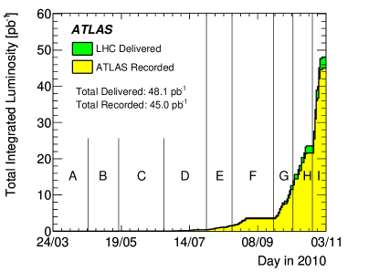
Figure 4: Profile with respect to time of the cumulative luminosity recorded by ATLAS during stable beams in $\sqrt{s}={7}{\mathrm{\ Te\kern-1.00006ptV}}$ $pp$ collisions (from the online luminosity measurement). The letters A-I refer to the data taking periods.

In order to compare trigger performance between data and MC simulation, a number of MC samples were generated. The MC samples used were produced using the PYTHIA pythia64 event generator with a parameter set ATLAS-MC09-Tune tuned to describe the underlying event and minimum bias data from Tevatron measurements at 0.63 TeV and 1.8 TeV. The generated events were processed through a GEANT4 geant4 based simulation of the ATLAS detector AtlasSim .

In some cases, where explicitly mentioned, performance results are shown for a subset of the data corresponding to a specific period of time. The 2010 run was split into data-taking periods; a new period being defined when there was a significant change in the detector conditions or instantaneous luminosity. The data-taking periods are summarized in Table 2. The rise in luminosity during the year was accompanied by an increase in the number of proton bunches injected into the LHC ring. From the end of September (Period G onwards) the protons were injected in bunch trains each consisting of a number of proton bunches separated by 150 ns.

3 Commissioning

In this section, the steps followed to commission the trigger are outlined and the trigger menus employed during the commissioning phase are described. The physics trigger menu, deployed in July 2010, is also presented and the evolution of the menu during the subsequent 2010 data-taking period is described.

3.1 Early Commissioning

The commissioning of the ATLAS trigger system started before the first LHC beam using cosmic ray events and, to commission L1, test pulses injected into the detector front-end electronics. To exercise the data acquisition system and HLT, simulated collision data were inserted into the ROS and processed through the whole online chain. This procedure provided the first full-scale test of the HLT selection software running on the online system.

The L1 trigger system was exercised for the first time with beam during single beam commissioning runs in 2008. Some of these runs included so-called splash events for which the proton beam was intentionally brought into collision with the collimators upstream from the experiment in order to generate very large particle multiplicities that could be used for detector commissioning. During this short period of single-beam data-taking, the HLT algorithms were tested offline.

Following the single beam data-taking in 2008, there was a period of cosmic ray data-taking, during which the HLT algorithms ran online. In addition to testing the selection algorithms used for collision data-taking, triggers specifically developed for cosmic ray data-taking were included. The latter were used to select and record a very large sample of cosmic ray events, which were invaluable for the commissioning and alignment of the detector sub-systems such as the inner detector and the muon spectrometer CosmicMuons .

3.2 Commissioning with colliding beams

Specialized commissioning trigger menus were developed for the early collision running in 2009 and 2010. These menus consisted mainly of L1-based triggers since the initial low interaction rate, of the order of a few Hz, allowed all events passing L1 to be recorded. Initially, the L1 MBTS trigger (Section 6.1) was unprescaled and acted as the primary physics trigger, recording all interactions. Once the luminosity exceeded $\sim 2\cdot 10^{27}\,\text{cm}^{-2}\text{s}^{-1}$, the L1 MBTS trigger was prescaled and the lowest threshold muon and calorimeter triggers became the primary physics triggers. With further luminosity increase, these triggers were also prescaled and higher threshold triggers, which were included in the commissioning menus in readiness, became the primary physics triggers. A coincidence with filled bunch crossing was required for the physics triggers. In addition, the menus contained non-collision triggers which required a coincidence with an empty or unpaired bunch crossing. For most of the lowest threshold physics triggers, a corresponding non-collision trigger was included in the menus to be used for background studies. The menus also contained a large number of supporting triggers needed for commissioning the L1 trigger system.

In the commissioning menus, event streaming was based on the L1 trigger categories. Three main inclusive physics streams were recorded: L1Calo for calorimeter-based triggers, L1Muon for triggers coming from the muon system and L1MinBias for events triggered by minimum bias detectors such as MBTS, LUCID and ZDC. In addition to these L1-based physics streams, the express stream was also recorded. Its content evolved significantly during the first weeks of data-taking. In the early data-taking, it comprised a random 10-20% of all triggered events in order to exercise the offline express stream processing system. Subsequently, the content was changed to enhance the proportion of electron, muon, and jet triggers. Finally, a small set of triggers of each trigger type was sent to the express stream. For each individual trigger, the fraction contributing to the express stream was adjustable by means of dedicated prescale values. The use of the express stream for data quality assessment and for calibration prior to offline reconstruction of the physics streams was commissioned during this period.

Table 3: Main calibration streams and their average event size per event. The average event size in the physics streams is 1.3 MB

Stream	Purpose	Event size [kB/event]
LArCells	LAr detector calibration	90
beamspot	Online beamspot determination	54
	based on Pixel and SCT detectors
IDTracks	ID alignment	20
PixelNoise, SCTNoise	Noise of the silicon detectors	38
Tile	Tile calorimeter calibration	221
Muon	Muon alignment	0.5
CostMonitoring	HLT system performance information	233
	including algorithm CPU usage

3.2.1 HLT commissioning

The HLT commissioning proceeded in several steps. During the very first collision data-taking at $\sqrt{s}={900}{\mathrm{\ Ge\kern-1.00006ptV}}$ in 2009, no HLT algorithms were run online. Instead they were exercised offline on collision events recorded in the express stream. Results were carefully checked to confirm that the trigger algorithms were functioning correctly and the algorithm execution times were evaluated to verify that timeouts would not occur during online running.

Table 4: Preliminary bandwidth allocations defined as guidelines to the various trigger groups, at three luminosity points, for an EF trigger rate of $\sim$200 Hz

	Luminosity [$\text{cm}^{-2}\text{s}^{-1}$]	$10^{30}$	$10^{31}$	$10^{32}$
Trigger Signature		Rate [Hz]	Rate [Hz]	Rate [Hz]
Minimum bias		20	10	10
Electron/Photon		30	45	50
Muon		30	30	50
Tau		20	20	15
Jet and forward jet		25	25	20
$b$-jet		10	15	10
$B$-physics		15	15	10
$E_{\mathrm{T}}^{\mathrm{miss}}$ and $\sum E_{\text{T}}$		15	15	10
Calibration triggers		30	13	13

After a few days of running offline, and having verified that the algorithms behaved as expected, the HLT algorithms were deployed online in monitoring mode. In this mode, the HLT algorithms ran online, producing trigger objects (e.g. calorimeter clusters and tracks) and a trigger decision at the HLT; however events were selected based solely on their L1 decision. Operating first in monitoring mode allowed each trigger to be validated before the trigger was put into active rejection mode. Recording the HLT objects and decision in each event allowed the efficiency of each trigger chain to be measured with respect to offline reconstruction. In addition a rejection factor, defined as input rate over output rate, could be evaluated for each trigger chain at L2 and EF. Running the HLT algorithms online also allowed the online trigger monitoring system to be exercised and commissioned under real circumstances.

Triggers can be set in monitoring or active rejection mode individually. This important feature allowed individual triggers to be put into active rejection mode as luminosity increased and trigger rates exceeded allocated maximum values. The first HLT trigger to be enabled for active rejection was a minimum bias trigger chain (mbSpTrk) based on a random bunch crossing trigger at L1 and an ID-based selection on track multiplicity at the HLT (Section 6.1). This trigger was already in active rejection mode in 2009.

Figure 5 illustrates the enabling of active HLT rejection during the first $\sqrt{s}={7}{\mathrm{\ Te\kern-1.00006ptV}}$ collision run, in March 2010. Since the HLT algorithms were disabled at the start of the run, the L1 and EF trigger rates were initially the same. The HLT algorithms were turned on, following rapid validation from offline processing, approximately two hours after the start of collisions, at about 15:00. All trigger chains were in monitoring mode apart from the mbSpTrk chain, which was in active rejection mode. However the random L1 trigger that forms the input to the mbSpTrk chain was disabled for the first part of the run and so the L1 and EF trigger rates remained the same until around 15:30 when this random L1 trigger was enabled. At this time there was a significant increase in the L1 rate, but the EF trigger rate stayed approximately constant due to the rejection by the mbSpTrk chain.

Figure 5: L1 and EF trigger rates during the first $\sqrt{s}={7}{\mathrm{\ Te\kern-1.00006ptV}}$ $pp$ collision run

Table 5: Examples of $p_{\mathrm{T}}$ thresholds and selections for the lowest unprescaled triggers in the physics menu at three luminosity values

	Luminosity [$cm^{-2}s^{-1}$]:	$3\times 10^{30}$	$2\times 10^{31}$	$2\times 10^{32}$
Category		$p_{\mathrm{T}}$ threshold [GeV], selection
Single muon		4, none	10, none	13,tight
Di-muon		4, none	6, none	6,loose
Single electron		10, medium	15, medium	15, medium
Di-electron		3, loose	5, medium	10, loose
Single photon		15, loose	30, loose	40, loose
Di-photon		5, loose	15, loose	15, loose
Single tau		20, loose	50, loose	84, loose
Single jet		30, none	75, loose	95, loose
$E_{\mathrm{T}}^{\mathrm{miss}}$		25, tight	30, loose	40,loose
$B$-physics		mu4_DiMu	mu4_DiMu	2mu4_DiMu

During the first months of 2010 data-taking, the LHC peak luminosity increased from $10^{27}\,\text{cm}^{-2}\text{s}^{-1}$ to $10^{29}\,\text{cm}^{-2}\text{s}^{-1}$. This luminosity was sufficiently low to allow the HLT to continue to run in monitoring mode and trigger rates were controlled by applying prescale factors at L1. Once the peak luminosity delivered by the LHC reached 1.2$\times$$10^{29}\,\text{cm}^{-2}\text{s}^{-1}$, it was necessary to enable HLT rejection for the highest rate L1 triggers. As luminosity progressively increased, more triggers were put into active rejection mode.

In addition to physics and commissioning triggers, a set of HLT-based calibration chains were also activated to produce dedicated data streams for detector calibration and monitoring. Table 3 lists the main calibration streams. These contain partial event data, in most cases data fragments from one sub-detector, in contrast to the physics streams which contain information from the whole detector.

3.3 Physics Trigger Menu

The end of July 2010 marked a change in emphasis from commissioning to physics. A physics trigger menu was deployed for the first time, designed for luminosities from $10^{30}\,\text{cm}^{-2}\text{s}^{-1}$ to $10^{32}\,\text{cm}^{-2}\text{s}^{-1}$. The physics trigger menu continued to evolve during 2010 to adapt to the LHC conditions. In its final form, it consisted of more than 470 triggers, the majority of which were primary and supporting physics triggers.

Figure 6: Profiles with respect to time of 6 the maximum instantaneous luminosity per day and 6 the peak mean number of interactions per bunch crossing (assuming a total inelastic cross section of 71.5 mb) recorded by ATLAS during stable beams in $\sqrt{s}={7}{\mathrm{\ Te\kern-1.00006ptV}}$ $pp$ collisions. Both plots use the online luminosity measurement

Figure 7: Comparison of online rates (solid) with offline rate predictions (hashed) at luminosity $10^{32}\,\text{cm}^{-2}\text{s}^{-1}$ for L1, L2, EF and main physics streams

In the physics menu, L1 commissioning items were removed, allowing for the addition of higher threshold physics triggers in preparation for increased luminosity. At the same time, combined triggers based on a logical “and” between two L1 items were introduced into the menu. Streaming based on the HLT decision was introduced and the corresponding L1-based streaming was disabled. In addition to calibration and express streams, data were recorded in the physics streams presented in Section 2. At the same time, preliminary bandwidth allocations were defined as guidelines for all trigger groups, as listed in Table 4.

The maximum instantaneous luminosity per day is shown in Fig. 6. As luminosity increased and the trigger rates approached the limits imposed by offline processing, primary and supporting triggers continued to evolve by progressively tightening the HLT selection cuts and by prescaling the lower $E_{\mathrm{T}}$ threshold triggers. Table 5 shows the lowest unprescaled threshold of various trigger signatures for three luminosity values.

In order to prepare for higher luminosities, tools to optimize prescale factors became very important. For example, the rate prediction tool uses enhanced bias data (data recorded with a very loose L1 trigger selection and no HLT selection) as input. Initially, these data were collected in dedicated enhanced bias runs using the lowest trigger thresholds, which were unprescaled at L1, and no HLT selection. Subsequently, enhanced bias triggers were added to the physics menu to collect the data sample during normal physics data-taking.

Figure 7 shows a comparison between online rates at $10^{32}\,\text{cm}^{-2}\text{s}^{-1}$ and predictions based on extrapolation from enhanced bias data collected at lower luminosity. In general online rates agreed with predictions within 10%. The biggest discrepancy was seen in rates from the JetTauEtmiss stream, as a result of the non-linear scaling of $E_{\mathrm{T}}^{\mathrm{miss}}$ and $\sum E_{\text{T}}$ trigger rates with luminosity, as shown later in Fig. 13. This non-linearity is due to in-time pile-up, defined as the effect of multiple $pp$ interactions in a bunch crossing. The maximum mean number of interactions per bunch crossing, which reached 3.5 in 2010, is shown as a function of day in Fig. 6. In-time pile-up had the most significant effects on the $E_{\mathrm{T}}^{\mathrm{miss}}$, $\sum E_{\text{T}}$(Section 6.6), and minimum bias (Section 6.1) signatures. Out-of-time pile-up is defined as the effect of an earlier bunch crossing on the detector signals for the current bunch crossing. Out-of-time pile-up did not have a significant effect in the 2010 $pp$ data-taking because the bunch spacing was 150 ns or larger.

4 Level 1

The Level 1 (L1) trigger decision is formed by the Central Trigger Processor (CTP) based on information from the calorimeter trigger towers and dedicated triggering layers in the muon system. An overview of the CTP, L1 calorimeter, and L1 muon systems and their performance follows. The CTP also takes input from the MBTS, LUCID and ZDC systems, described in Section 6.1.

Figure 8: L1 live fraction per run throughout the full data-taking period of 2010, as used for luminosity estimates for correcting trigger dead-time effects. The live fraction is derived from the trigger L1_MBTS_2

4.1 Central Trigger Processor

The CTP DetectorPaper ; Ask:2008zz forms the L1 trigger decision by applying the multiplicity requirements and prescale factors specified in the trigger menu to the inputs from the L1 trigger systems. The CTP also provides random triggers and can apply specific LHC bunch crossing requirements. The L1 trigger decision is distributed, together with timing and control signals, to all ATLAS sub-detector readout systems.

The timing signals are defined with respect to the LHC bunch crossings. A bunch crossing is defined as a 25 ns time-window centred on the instant at which a proton bunch may traverse the ATLAS interaction point. Not all bunch crossings contain protons; those that do are called filled bunches. In 2010, the minimum spacing between filled bunches was 150 ns. In the nominal LHC configuration, there are a maximum of 3564 bunch crossings per LHC revolution. Each bunch crossing is given a bunch crossing identifier (BCID) from 0 to 3563. A bunch group consists of a numbered list of BCIDs during which the CTP generates an internal trigger signal. The bunch groups are used to apply specific requirements to triggers such as paired (colliding) bunches for physics triggers, single (one-beam) bunches for background triggers, and empty bunches for cosmic ray, noise and pedestal triggers.

4.1.1 Dead-time

Following an L1 accept the CTP introduces dead-time, by vetoing subsequent triggers, to protect front-end readout buffers from overflowing. This preventive dead-time mechanism limits the minimum time between two consecutive L1 accepts (simple dead-time), and restricts the number of L1 accepts allowed in a given period (complex dead-time). In 2010 running, the simple dead-time was set to 125 ns and the complex dead-time to 8 triggers in $80~{}\mu$s. This preventative dead-time is in addition to busy dead-time which can be introduced by ATLAS sub-detectors to temporarily throttle the trigger rate.

The CTP monitors the total L1 trigger rate and the rates of individual L1 triggers. These rates are monitored before and after prescales and after dead-time related vetoes have been applied. One use of this information is to provide a measure of the L1 dead-time, which needs to be accounted for when determining the luminosity. The L1 dead-time correction is determined from the live fraction, defined as the ratio of trigger rates after CTP vetoes to the corresponding trigger rates before vetoes. Figure 8 shows the live fraction based on the L1_MBTS_2 trigger (Section 6.1), the primary trigger used for these corrections in 2010. The bulk of the data were recorded with live fractions in excess of 98%. As a result of the relatively low L1 trigger rates and a bunch spacing that was relatively large ($\geq 150$ ns) compared to the nominal LHC spacing (25 ns), the preventive dead-time was typically below $10^{-4}$ and no bunch-to-bunch variations in dead-time existed.

Figure 9: L1 dead-time fractions per bunch crossing for a LHC test fill with a 50 ns bunch spacing. The dead-time fractions as a function of BCID (left), taking a single bunch train of 12 bunches as an example and a histogram of the individual dead-time fractions for each paired bunch crossing (right). The paired bunch crossings (odd-numbered BCID from 945 to 967) are indicated by vertical dashed lines on the left hand plot

Towards the end of the 2010 data-taking a test was performed with a fill of bunch trains with 50 ns spacing, the running mode expected for the bulk of 2011 data-taking. The dead-time measured during this test is shown as a function of BCID in Fig. 9, taking a single bunch train as an example. The first bunch of the train (BCID 945) is only subject to sub-detector dead-time of $\sim$0.1%, while the following bunches in the train (BCIDs 947 to 967) are subject to up to 4% dead-time as a result of the preventative dead-time generated by the CTP. The variation in dead-time between bunch crossings will be taken into account when calculating the dead-time corrections to luminosity in 2011 running.

4.1.2 Rates and Timing

Figure 10 shows the trigger rate for the whole data-taking period of 2010, compared to the luminosity evolution of the LHC. The individual rate points are the average L1 trigger rates in ATLAS runs with stable beams, and the luminosity points correspond to peak values for the run. The increasing selectivity of the trigger during the course of 2010 is illustrated by the fact that the L1 trigger rate increased by one order of magnitude; whereas, the peak instantaneous luminosity increased by five orders of magnitude. The L1 trigger system was operated at a maximum trigger rate of just above 30 kHz, leaving more than a factor of two margin to the design rate of 75 kHz.

Figure 10: Evolution of the L1 trigger rate throughout 2010 (lower panel), compared to the instantaneous luminosity evolution (upper panel)

The excellent level of synchronization of L1 trigger signals in time is shown in Fig. 11 for a selection of L1 triggers. The plot represents a snapshot taken at the end of October 2010. Proton-proton collisions in nominal filled paired bunch crossings are defined to occur in the central bin at 0. As a result of mistiming caused by alignment of the calorimeter pulses that are longer than a single bunch crossing, trigger signals may appear in bunch crossings preceding or succeeding the central one. In all cases mistiming effects are below $10^{-3}$. The timing alignment procedures for the L1 calorimeter and L1 muon triggers are described in Section 4.2 and Section 4.3 respectively.

4.2 L1 Calorimeter Trigger

The L1 calorimeter trigger L1CaloPaper is based on inputs from the electromagnetic and hadronic calorimeters covering the region $|\eta|<4.9$. It provides triggers for localized objects (e.g. electron/photon, tau and jet) and global transverse energy triggers. The pipelined processing and logic is performed in a series of custom built hardware modules with a latency of less than 1 $\mu$s. The architecture, calibration and performance of this hardware trigger are described in the following sub-sections.

Figure 11: L1 trigger signals in units of bunch crossings for a number of triggers. The trigger signal time is plotted relative to the position of filled paired bunches for a particular data-taking period towards the end of the 2010 $pp$ run

4.2.1 L1 Calorimeter Trigger Architecture

The L1 calorimeter trigger decision is based on dedicated analogue trigger signals provided by the ATLAS calorimeters independently from the signals read out and used at the HLT and offline. Rather than using the full granularity of the calorimeter, the L1 decision is based on the information from analogue sums of calorimeter elements within projective regions, called trigger towers. The trigger towers have a size of approximately $\Delta\eta\times\Delta\phi=0.1\times 0.1$ in the central part of the calorimeter, $|\eta|<2.5$, and are larger and less regular in the more forward region. Electromagnetic and hadronic calorimeters have separate trigger towers.

The 7168 analogue inputs must first be digitized and then associated to a particular LHC bunch crossing. Much of the tuning of the timing and transverse energy calibration was performed during the 2010 data-taking period since the final adjustments could only be determined with colliding beam events. Once digital transverse energies per LHC bunch crossing are formed, two separate processor systems, working in parallel, run the trigger algorithms. One system, the cluster processor uses the full L1 trigger granularity information in the central region to look for small localized clusters typical of electron, photon or tau particles. The other, the jet and energy-sum processor, uses $2\times 2$ sums of trigger towers, called jet elements, to identify jet candidates and form global transverse energy sums: missing transverse energy, total transverse energy and jet-sum transverse energy. The magnitude of the objects and sums are compared to programmable thresholds to form the trigger decision. The thresholds used in 2010 are shown in Table 1 in Section 2.

Figure 12: Building blocks of the electron/photon and tau algorithms with the sums to be compared to programmable thresholds

The details of the algorithms can be found elsewhere L1CaloPaper and only the basic elements are described here. Figure 12 illustrates the electron/photon and tau triggers as an example. The electron/photon trigger algorithm identifies an Region of Interest as a $2\times 2$ trigger tower cluster in the electromagnetic calorimeter for which the transverse energy sum from at least one of the four possible pairs of nearest neighbour towers ($1\times 2$ or $2\times 1$) exceeds a pre-defined threshold. Isolation-veto thresholds can be set for the 12-tower surrounding ring in the electromagnetic calorimeter, as well as for hadronic tower sums in a central $2\times 2$ core behind the cluster and the 12-tower hadronic ring around it. Isolation requirements were not applied in 2010 running. Jet RoIs are defined as $4\times 4$, $6\times 6$ or $8\times 8$ trigger tower windows for which the summed electromagnetic and hadronic transverse energy exceeds pre-defined thresholds and which surround a $2\times 2$ trigger tower core that is a local maximum. The location of this local maximum also defines the coordinates of the jet RoI.

The real-time output to the CTP consists of more than 100 bits per bunch crossing, comprising the coordinates and threshold bits for each of the RoIs and the counts of the number of objects (saturating at seven) that satisfy each of the electron/photon, tau and jet criteria.

4.2.2 L1 Calorimeter Trigger Commissioning and Rates

After commissioning with cosmic ray and collision data, including event-by-event checking of L1 trigger results against offline emulation of the L1 trigger logic, the calorimeter trigger processor ran stably and without any algorithmic errors. Bit-error rates in digital links were less than 1 in $10^{20}$. Eight out of 7168 trigger towers were non-operational in 2010 due to failures in inaccessible analogue electronics on the detector. Problems with detector high and low voltage led to an additional $\sim$1% of trigger towers with low or no response. After calibration adjustments, L1 calorimeter trigger conditions remained essentially unchanged for 99% of the 2010 proton-proton integrated luminosity.

Figure 13: L1 trigger rate scaling for some low threshold trigger items as a function of luminosity per bunch crossing. The rate for XE10 has been scaled by 0.2

The scaling of the L1 trigger rates with luminosity is shown in Fig. 13 for some of the low-threshold calorimeter trigger items. The localised objects, such as electrons and jet candidates, show an excellent linear scaling relationship with luminosity over a wide range of luminosities and time. Global quantities such as the missing transverse energy and total transverse energy triggers also scale in a smooth way, but are not linear as they are strongly affected by in-time pile-up which was present in the later running periods.

4.2.3 L1 Calorimeter Trigger Calibration

In order to assign the calorimeter tower signals to the correct bunch crossing, a task performed by the bunch crossing identification logic, the signals must be synchronized to the LHC clock phase with nanosecond precision. The timing synchronization was first established with calorimeter pulser systems and cosmic ray data and then refined using the first beam delivered to the detector in the splash events (Section 3). During the earliest data-taking in 2010 the correct bunch crossing was determined for events with transverse energy above about 5 GeV. Timing was incrementally improved, and for the majority of the 2010 data the timing of most towers was better than ${\pm}2$ ns, providing close to ideal performance.

In order to remove the majority of fake triggers due to small energy deposits, signals are processed by an optimized filter and a noise cut of around 1.2 GeV is applied to the trigger tower energy. The efficiency for an electromagnetic tower energy to be associated to the correct bunch crossing and pass this noise cut is shown in Fig. 14 as a function of the sum of raw cell $E_{\mathrm{T}}$ within that tower, for different regions of the electromagnetic calorimeter. The efficiency turn-on is consistent with the optimal performance expected from a simulation of the signals and the full efficiency in the plateau region indicates the successful association of these small energy deposits to the correct bunch crossing.

Special treatment, using additional bunch crossing identification logic, is needed for saturated pulses with $E_{\mathrm{T}}$ above about 250 GeV. It was shown that BCID logic performance was more than adequate for 2010 LHC energies, working for most trigger towers up to transverse energies of 3.5 TeV and beyond. Further tuning of timing and algorithm parameters will ensure that the full LHC energy range is covered.

Figure 14: Efficiency for an electromagnetic trigger tower energy to be associated with the correct bunch crossing and pass a noise cut of around 1.2 GeVas a function of the sum of raw cell $E_{\mathrm{T}}$ within that tower

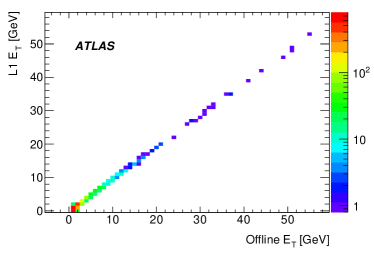
Figure 15: Typical transverse energy correlation plots for two individual central calorimeter towers, 15 electromagnetic and 15 hadronic

In order to obtain the most precise transverse energy measurements, a transverse energy calibration must be applied to all trigger towers. The initial transverse energy calibration was produced by calibration pulser runs. In these runs signals of a controlled size are injected into the calorimeters. Subsequently, with sufficient data, the gains were recalibrated by comparing the transverse energies from the trigger with those calculated offline from the full calorimeter information. By the end of the 2010 data-taking this analysis had been extended to provide a more precise calibration on a tower-by-tower basis. In most cases, the transverse energies derived from the updated calibration differed by less than 3% from those obtained from the original pulser-run based calibration. Examples of correlation plots between trigger and offline calorimeter transverse energies can be seen in Fig. 15. In the future, with even larger datasets, the tower-by-tower calibration will be further refined based on physics objects with precisely known energies, for example, electrons from $Z$ boson decays.

4.3 L1 Muon Trigger

Figure 16: A section view of the L1 muon trigger chambers. TCG I was not used in the trigger in 2010

The L1 muon trigger system DetectorPaper ,CSCBook is a hardware-based system to process input data from fast muon trigger detectors. The system’s main task is to select muon candidates and identify the bunch crossing in which they were produced. The primary performance requirement is to be efficient for muon $p_{\mathrm{T}}$ thresholds above 6 GeV. A brief overview of the L1 muon trigger is given here; the performance of the muon trigger is presented in Section 6.3.

4.3.1 L1 Muon Trigger Architecture

Muons are triggered at L1 using the RPC system in the barrel region ($|\eta|<1.05$) and the TGC system in the end-cap regions ($1.05<|\eta|<2.4$), as shown in Fig. 16. The RPC and TGC systems provide rough measurements of muon candidate $p_{\mathrm{T}}$, $\eta$, and $\phi$. The trigger chambers are arranged in three planes in the barrel and three in each endcap (TCG I shown in Fig. 16 did not participate in the 2010 trigger). Each plane is composed of two to four layers. Muon candidates are identified by forming coincidences between the muon planes. The geometrical coverage of the trigger in the end-caps is $\approx 99$%. In the barrel the coverage is reduced to $\approx 80\%$ due to a crack around $\eta=0$, the feet and rib support structures for the ATLAS detector and two small elevators in the bottom part of the spectrometer.

The L1 muon trigger logic is implemented in similar ways for both the RPC and TCG systems, but with the following differences:

• The planes of the RPC system each consist of a doublet of independent detector layers, each read out in the $\eta$ ($z$) and $\phi$ coordinates. A low-$p_{\mathrm{T}}$ trigger is generated by requiring a coincidence of hits in at least 3 of the 4 layers of the inner two planes, labelled as RPC1 and RPC2 in Fig. 16). The high-$p_{\mathrm{T}}$  logic starts from a low-$p_{\mathrm{T}}$  trigger, then looks for hits in one of the two layers of the high-$p_{\mathrm{T}}$ confirmation plane (RPC3).

• The two outermost planes of the TGC system (TGC2 and TGC3) each consist of a doublet of independent detectors read out by strips to measure the $\phi$ coordinate and wires to measure the $\eta$ coordinate. A low-$p_{\mathrm{T}}$ trigger is generated by a coincidence of hits in at least 3 of the 4 layers of the outer two planes. The inner plane (TGC1) contains 3 detector layers, the wires are read out from all of these, but the strips from only 2 of the layers. The high-$p_{\mathrm{T}}$ trigger requires at least one of two $\phi$-strip layers and 2 out of 3 wire layers from the innermost plane in coincidence with the low-$p_{\mathrm{T}}$ trigger.

In both the RPC and TGC systems, coincidences are generated separately for $\eta$ and $\phi$ and can then be combined with programmable logic to form the final trigger result. The configuration for the 2010 data-taking period required a logical AND between the $\eta$ and $\phi$ coincidences in order to have a muon trigger.

In order to form coincidences, hits are required to lie within parametrized geometrical muon roads. A road represents an envelope containing the trajectories, from the nominal interaction point, of muons of either charge with a $p_{\mathrm{T}}$ above a given threshold. Example roads are shown in Fig. 16. There are six programmable $p_{\mathrm{T}}$ thresholds at L1 (see Table 1) which are divided into two sets: three low-$p_{\mathrm{T}}$ thresholds to cover values up to 10 GeV, and three high-$p_{\mathrm{T}}$ thresholds to cover $p_{\mathrm{T}}$ greater than 10 GeV.

To enable the commissioning and validation of the performance of the system for 2010 running, two triggers were defined which did not require coincidences within roads and thus gave maximum acceptance and minimum trigger bias. One (MU0) based on low-$p_{\mathrm{T}}$ logic and the other (MU0_COMM) based on the high-$p_{\mathrm{T}}$ logic. For these triggers the only requirement was that hits were in the same trigger tower ($\eta~{}\times~{}\phi~{}\sim~{}$0.1$~{}\times~{}$0.1).

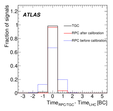
Figure 17: The timing alignment with respect to the LHC bunch clock (25 ns units) for the RPC system (before and after the timing calibration) and the TGC system

4.3.2 L1 Muon Trigger Timing Calibration

In order to assign the hit information to the correct bunch crossing, a precise alignment of RPC and TGC signals, or timing calibration, was performed to take into account signal delays in all components of the read out and trigger chain. Test pulses were used to calibrate the TGC timing to within 25 ns (one bunch crossing) before the start of data-taking. Tracks from cosmic ray and collision data were used to calibrate the timing of the RPC system. This calibration required a sizable data sample to be collected before a time alignment of better than 25 ns was reached. As described in section 4.1, the CTP imposes a 25 ns window about the nominal bunch crossing time during which signals must arrive in order to contribute to the trigger decision. In the first phase of the data-taking, while the timing calibration of the RPC system was on-going, a special CTP configuration was used to increase the window for muon triggers to 75 ns. The majority of 2010 data were collected with both systems aligned to within one bunch crossing for both high-$p_{\mathrm{T}}$ and low-$p_{\mathrm{T}}$ triggers. In Fig. 17  the timing alignment of the RPC and TGC systems is shown with respect to the LHC bunch clock in units of the 25 ns bunch crossings (BC).

5 High Level Trigger Reconstruction

The HLT has additional information available, compared to L1, including inner detector hits, full information from the calorimeter and data from the precision muon detectors. The HLT trigger selection is based on features reconstructed in these systems. The reconstruction is performed, for the most part, inside RoIs in order to minimize execution times and reduce data requests across the network at L2. The sections below give a brief description of the algorithms for inner detector tracking, beamspot measurement, calorimeter clustering and muon reconstruction. The performance of the algorithms is presented, including measurements of execution times which meet the timing constraints outlined in Section 2.

5.1 Inner Detector Tracking

The track reconstruction in the Inner Detector is an essential component of the trigger decision in the HLT. A robust and efficient reconstruction of particle trajectories is a prerequisite for triggering on electrons, muons, $B$-physics, taus, and $b$-jets. It is also used for triggering on inclusive $pp$ interactions and for the online determination of the beamspot (Section 5.2), where the reconstructed tracks provide the input to reconstruction of vertices. This section gives a short description of the reconstruction algorithms and an overview of the performance of the track reconstruction with a focus on tracking efficiencies in the ATLAS trigger system.

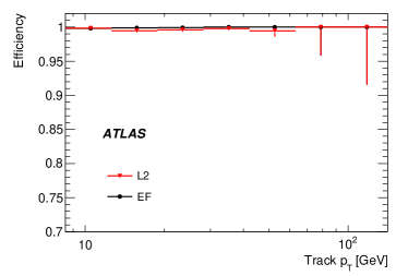
Figure 18: L2 and EF tracking reconstruction efficiency with respect to offline 18 muon candidates and 18 electron candidates

Figure 19: L2 and EF tracking reconstruction efficiency with respect to offline reference tracks inside 19 tau RoIs and 19 jet RoIs

5.1.1 Inner Detector Tracking Algorithms

The L2 reconstruction algorithms are specifically designed to meet the strict timing requirements for event processing at L2. The track reconstruction at the EF is less time constrained and can use, to a large extent, software components from the offline reconstruction. In both L2 and EF the track finding is preceded by a data preparation step in which detector data are decoded and transformed to a set of hit positions in the ATLAS coordinate system. Clusters are first formed from adjacent signals on the SCT strips or in the Pixel detector. Two-dimensional Pixel clusters and pairs of one-dimensional SCT clusters (from back-to-back detectors rotated by a small stereo angle with respect to one another) are combined with geometrical information to provide three-dimensional hit information, called space-points. Clusters and space-points provide the input to the HLT pattern recognition algorithms.

The primary track reconstruction strategy is inside-out tracking which starts with pattern recognition in the SCT and Pixel detectors; track candidates are then extended to the TRT volume. In addition, the L2 has an algorithm that reconstructs tracks in the TRT only and the EF has an additional track reconstruction strategy that is outside-in, starting from the TRT and extending the tracks to the SCT and Pixel detectors.

Track reconstruction at both L2 and EF is run in an RoI-based mode for electron, muon, tau and $b$-jet signatures. $B$-physics signatures are based either on a FullScan (FS) mode (using the entire volume of the Inner Detector) or a large RoI. The tracking algorithms can be configured differently for each signature in order to provide the best performance.

L2 uses two different pattern recognition strategies:

• A three-step histogramming technique, called IdScan. First, the $z$-position of the primary vertex, $z_{v}$, is determined as follows. The RoI is divided into $\phi$-slices and $z$-intercept values are calculated and histogrammed for lines through all possible pairs of space-points in each $phi$-slice; $z_{v}$ is determined from peaks in this histogram. The second step is to fill a $(\eta,\phi)$ histogram with values calculated with respect to $z_{v}$ for each space-point in the RoI; groups of space-points to be passed on to the third step are identified from histogram bins containing at least four space-points from different detector layers. In the third step, a $(1/p_{\mathrm{T}},\phi)$ histogram is filled from values calculated for all possible triplets of space-points from different detector layers; track candidates are formed from bins containing at least four space-points from different layers. This technique is the approach used for electron, muon and $B$-physics triggers due to the slightly higher efficiency of IdScan relative to SiTrack.

• A combinatorial technique, called SiTrack. First, pairs of hits consistent with a beamline constraint are found within a subset of the inner detector layers. Next, triplets are formed by associating additional hits in the remaining detector layers consistent with a track from the beamline. In the final step, triplets consistent with the same track trajectory are merged, duplicate or outlying hits are removed and the remaining hits are passed to the track fitter. SiTrack is the approach used for tau and jet triggers as well as the beamspot measurement as it has a slightly lower fake-track fraction.

In both cases, track candidates are further processed by a common Kalman bib:KalmanFitter filter track fitter and extended to the TRT for an improved $p_{\mathrm{T}}$ resolution and to benefit from the electron identification capability of the TRT.

The EF track reconstruction is based on software shared with the offline reconstruction bib:newtracking . The offline software was extended to run in the trigger environment by adding support for reconstruction in an RoI-based mode. The pattern recognition in the EF starts from seeds built from triplets of space-points in the Pixel and SCT detectors. Triplets consist of space-points from different layers, all in the pixel detector, all in the the SCT or two space-points in the pixel detector and one in the SCT. Seeds are preselected by imposing a minimum requirement on the momentum and a maximum requirement on the impact parameters. The seeds define a road in which a track candidate can be formed by adding additional clusters using a combinatorial Kalman filter technique. In a subsequent step, the quality of the track candidates is evaluated and low quality candidates are rejected. The tracks are then extended into the TRT and a final fit is performed to extract the track parameters.

5.1.2 Inner Detector Tracking Algorithms Performance

Figure 20: The RMS of the core 95% (RMS₉₅) of the inverse-$p_{\mathrm{T}}$ residual as a function of offline track $\eta$

The efficiency of the tracking algorithms is studied using specific monitoring triggers, which do not require a track to be present for the event to be accepted, and are thus unbiased for track efficiency measurements. The efficiency is defined as the fraction of offline reference tracks that are matched to a trigger track (with matching requirement $\Delta R=\sqrt{\Delta\phi^{2}+\Delta\eta^{2}}<0.1$). Offline reference tracks are required to have $|\eta|<2.5$, $|d_{0}|<1.5$ mm, $|z_{0}|<200$ mm and $|(z_{0}-z_{V})\sin{\theta}|<1.5$ mm, where $d_{0}$ and $z_{0}$ are the transverse and longitudinal impact parameters, and $z_{V}$ is the position of the primary vertex along the beamline as reconstructed offline. The reference tracks are also required to have one Pixel hit and at least six SCT clusters. For tau and jet RoIs, the reference tracks are additionally required to have $\chi^{2}$ probability of the track fit higher than 1%, two Pixel hits, one in the innermost layer, and a total of at least seven SCT clusters.

The L2 and EF tracking efficiencies are shown as a function of $p_{\mathrm{T}}$ for offline muon candidates in Fig. 18 and for offline electron candidates in Fig. 18. Tracking efficiencies in tau and jet RoIs are shown in Fig. 19, determined with respect to all offline reference tracks lying within the RoI. In all cases, the efficiency is close to 100% in the $p_{\mathrm{T}}$ range important for triggering.

The RMS of the core 95% (RMS₉₅) of the inverse-$p_{\mathrm{T}}$ residual $((\frac{1}{p_{\mathrm{T}}})^{\mathrm{trigger}}-(\frac{1}{p_{\mathrm{T}}})^{\mathrm{offline}})$ distribution is shown as a function of $\eta$ in Fig. 20. Both L2 and EF show good agreement with offline, although the residuals between L2 and offline are larger, particularly at high $|\eta|$  as a consequence of the speed-optimizations made at L2. Figure 21 shows the residuals in $d_{0}$, $\phi$ and $\eta$. Since it uses offline software, EF tracking performance is close to that of the offline reconstruction. Performance is not identical, however, due to an online-specific configuration of offline software designed to increase speed and be more robust to compensate for the more limited calibration and detector status information available in the online environment.

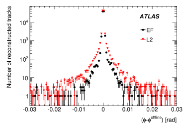
Figure 21: Residuals with respect to offline for track parameters 21 $d_{0}$, 21 $\phi$ and 21 $\eta$

5.1.3 Inner Detector Tracking Algorithms Timing

Distributions of the algorithm execution time at L2 and EF are shown in Fig. 22. The total time for L2 reconstruction is shown in Fig. 22 for a muon algorithm in RoI and FullScan mode. The times of the different reconstruction steps at the EF are shown in Fig. 22 for muon RoIs and in Fig. 22 for FullScan mode. The execution times are shown for all instances of the algorithm execution, whether the trigger was passed or not. The execution times are well within the online constraints.

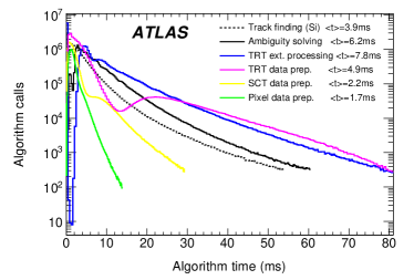
Figure 22: Execution times for 22 FullScan reconstruction and reconstruction within muon RoIs at L2, 22 the different EF reconstruction steps in muon RoIs and 22 the different steps of the EF FullScan. The mean time of each algorithm is marked in the legend. The structure in the TRT data preparation time in 22 is due to caching

5.2 Beamspot

The online beamspot measurement uses L2 ID tracks from the SiTrack algorithm (Section 5.1) to reconstruct primary vertices on an event-by-event basis bib:beamspotconfnote . The vertex position distributions collected over short time intervals are used to measure the position and shape of the luminous region, beamspot, parametrized by a three-dimensional Gaussian. The coordinates of the centroids of reconstructed vertices determine the average position of the collision point in the ATLAS coordinate system as well as the size and orientation of the ellipsoid representing the luminous region in the horizontal ($x$-$z$) and vertical ($y$-$z$) planes.

These observables are continuously reconstructed and monitored online in the HLT, and communicated, for each luminosity block, to displays in the control room. In addition, the instantaneous rate of reconstructed vertices can be used online as a luminosity monitor. Following these online measurements, a system for applying real-time configuration changes to the HLT farm distributes updates for use by trigger algorithms that depend on the precise knowledge of the luminous region, such as $b$-jet tagging (Section 6.7).

Figure 23: A timeline of the observed collision point centroid position relative to the nominal beam position

Figure 23 shows the variation of the collision point centroid around the nominal beam position in the transverse plane ($y_{nominal}$) over a period of a few weeks. The nominal beam position, which is typically up to several hundred microns from the centre of the ATLAS coordinate system, is defined by a time average of previous measured centroid positions. The figure shows that updates distributed to the online system as a part of the feedback mechanism take account of the measured beam position within a narrow band of only a few microns. The large deviations on Oct 4 and Sept 22 are from beam-separation scans.

During 2010 data-taking, beamspot measurements were averaged over the entire period of stable beam during a run and updates applied, for subsequent runs, in the case of significant shifts. For 2011 running, when triggers that are sensitive to the beamspot position, such as the $b$-jet trigger (Section 6.7), are activated, updates will be made more frequently.

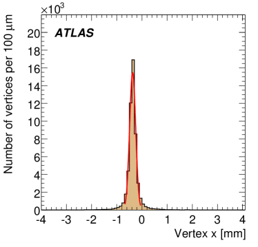
Figure 24: The distribution of primary vertices reconstructed by the online beamspot algorithm in an example run for vertices with at least two tracks ($p_{\mathrm{T}}>0.5{\mathrm{\ Ge\kern-1.00006ptV}}$ and $|\eta|<2.5$) in 24 the transverse plane, 24 $x$, 24 $y$, and 24 $z$. The mean beam position and observed widths, before correction for the intrinsic vertex position resolution; $\mu_{x}=(-0.370\pm 0.001)$mm, $\sigma_{x}=(0.120\pm 0.001)$mm, $\mu_{y}=(0.628\pm 0.001)$mm, $\sigma_{y}=(0.132\pm 0.001)$mm, $\mu_{z}=(1.03\pm 0.10)$mm, $\sigma_{z}=(22.14\pm 0.07)$mm

5.2.1 Beamspot Algorithm

The online beamspot algorithm employs a fast vertex fitter able to efficiently fit the L2 tracks emerging from the interaction region to common vertices within a fraction of the L2 time budget. The tracks used for the vertex fits are required to have at least one Pixel space-point and three SCT space-points and a transverse impact parameter with respect to the nominal beamline of $|d_{0}|<1$ cm. Clusters of tracks with similar impact parameter ($z_{0}$) along the nominal beamline form the input to the vertex fits. The tracks are ordered in $p_{\mathrm{T}}$ and the highest-$p_{\mathrm{T}}$ track above 0.7 GeV is taken as a seed. The seed track is grouped with all other tracks with $p_{\mathrm{T}}>0.5{\mathrm{\ Ge\kern-1.00006ptV}}$ within $\Delta z_{0}<1$ cm. The average $z_{0}$ value of the tracks in the group provides the initial estimate of the vertex position in the longitudinal direction, used as a starting point for the vertex fitter. In order to find additional vertices in the event, the process is repeated taking the next highest $p_{\mathrm{T}}$ track above 0.7 GeV as the seed.

5.2.2 Beamspot Algorithm Performance

Using the event-by-event vertex distribution computed in real-time by the HLT and accumulated in intervals of typically two minutes, the position, size and tilt angles of the luminous region within the ATLAS coordinate system are measured. A view of the transverse distribution of vertices reconstructed by the HLT is shown in Fig. 24 along with the transverse ($x$ and $y$) and longitudinal ($z$) profiles.

The measurement of the true size of the beam relies on an unfolding of the intrinsic resolution of the vertex position measurement. A correction for the intrinsic resolution is determined, in real-time, by measuring the distance between two daughter vertices constructed from a primary vertex when its tracks are split into two random sets for re-fitting. This correction method has the benefit that it allows the determination of the beam width to be relatively independent of variations in detector resolution, by explicitly taking the variation into account.

Figure 25: The corrected width of the measured vertex position, in $x$, along with the measured intrinsic resolution and the raw measured width before correction for the resolution. The asymptotic value of the corrected width provides a measurement of the true beam width

Figure 25 shows the measured beam width, in x, as a function of the number of tracks per vertex. The raw measured width is shown as well as the width after correction for the intrinsic resolution of the vertex position measurement. The measured intrinsic resolution is also shown. The intrinsic resolution is overestimated, and hence the corrected width is underestimated, for vertices with a small number of tracks. The true beam width ($50\mu$m) is, therefore, given by the asymptotic value of the corrected width. For this reason vertices used for the beam width measurement are required to have more than a minimum number of tracks. The value of this cut depends on the beamspot size. Data and MC studies have shown that intrinsic resolution must be less than about two times the beamspot size to be measured. For the example fill shown in Fig. 25, this requirement corresponds to $\gtrsim 10$ tracks per vertex. To resolve smaller beam sizes, the multiplicity requirement can be raised accordingly.

5.3 Calorimeter

The calorimeter reconstruction algorithms are designed to reconstruct clusters of energy from electrons, photons, taus and jet objects using calorimeter cell information. At the EF, global $E_{\mathrm{T}}^{\mathrm{miss}}$ is also calculated. Calorimeter information is also used to provide information to the muon isolation algorithms.

At L2, custom algorithms are used to confirm the results of the L1 trigger and provide cluster information as input to the signature-specific selection algorithms. The detailed calorimeter cell information available at the HLT allows the position and transverse energy of clusters to be calculated with higher precision than at L1. In addition, shower shape variables useful for particle identification are calculated. At the EF, offline algorithms with custom interfaces for online running are used to reproduce offline clustering performance as closely as possible, using similar calibration procedures. More details on the HLT and offline clustering algorithms can be found in Ref. CSCBook ; ATL-LARG-PUB-2008-002 .

Figure 26: Residuals between online and offline $E_{\mathrm{T}}$ values for EM clustering at 26 L2 and 26 EF

5.3.1 Calorimeter Algorithms

While the clustering tools used in the trigger are customized for the different signatures, they take their input from a common data preparation software layer. This layer, which is common to L2 and the EF, requests data using the general trigger framework tools and drives sub-detector specific code to convert the digital information into the input objects (calorimeter cells with energy and geometry) used by the algorithms. This code is optimized to guarantee fast unpacking of detector data. The data is organized so as to allow efficient access by the algorithms. At the EF the calorimeter cell information is arranged using projective regions called towers, of size $\Delta\eta\times\Delta\phi=0.025\times 0.025$ for EM clustering and $\Delta\eta\times\Delta\phi=0.1\times 0.1$ for jet algorithms.

The L2 electron and photon ($e/\gamma$) algorithm performs clustering withing an RoI of dimension $\Delta\eta\times\Delta\phi=0.4\times 0.4$. The algorithm relies on the fact that most of the energy from an electron or photon is deposited in the second layer of the electromagnetic (EM) calorimeter. The cell with the most energy in this layer provides the seed to the clustering process. This cell defines the centre of a $\Delta\eta\times\Delta\phi=0.075\times 0.125$ window within this layer. The cluster position is calculated by taking an energy-weighted average of cell positions within this window and the cluster transverse energy is calculated by summing the cell transverse energies within equivalent windows in all layers. Subsequently, a correction for the upstream energy loss and for lateral and longitudinal leakage is applied.

At the EF a clustering algorithm similar to the offline algorithm is used. Cluster finding is performed using a sliding window algorithm acting on the towers formed in the data preparation step. Fixed window clusters in regions of $\Delta\eta\times\Delta\phi=0.075\times 0.175~{}(0.125\times 0.125)$ are built in the barrel (end-caps). The cluster transverse energy and position are calculated in the same way as at L2. Distributions of $E_{\mathrm{T}}$ residuals, defined as the fractional difference between online and offline $E_{\mathrm{T}}$ values, are shown in Fig. 26 for L2 and EF. The broader L2 distribution is a consequence of the specialized fast algorithm used at L2.

Figure 27: Tau EF $E_{\mathrm{T}}$ residuals with respect to offline

The L2 tau clustering algorithm searches for a seed in all EM and hadronic calorimeter layers and within an RoI of $\Delta\eta\times\Delta\phi=0.6\times 0.6$. At the EF the calorimeter cells within a $\Delta\eta\times\Delta\phi=0.8\times 0.8$ region are used directly as input to a topological clustering algorithm that builds clusters of any shape by adding neighbouring cells that have energy above a given number (0-4) of standard deviations of the noise distribution. The large RoI size is motivated by the cluster size used in offline tau reconstruction. The EF tau $E_{\mathrm{T}}$ residual with respect to the offline clustering algorithm is shown in Fig. 27.

Figure 28: Residuals between L2 and offline values of jet cluster 28 $\phi$ and 28 $\eta$ shown for data and MC simulation. The anti-$k_{\mathrm{T}}$ algorithm with R=0.4 was used for offline clustering

The L2 jet reconstruction uses a cone algorithm iterating over cells in a relatively large RoI ($\Delta\eta\times\Delta\phi=1.0\times 1.0$). Figure 28 shows L2 $\phi$ and $\eta$ residuals with respect to offline, showing reasonable agreement with simulation. The asymmetry, which is reproduced by the simulation, is due to the fact that L2 jet reconstruction, unlike offline, is performed within an RoI whose position is defined with the granularity of the L1 jet element size (Section 4.2). The L2 jet $E_{\mathrm{T}}$ reconstruction and jet energy scale are discussed further in Section 6.4. During 2010, EF jet trigger algorithms ran online in monitoring mode i.e. without rejection. In 2011, the EF jet selection will be activated based on EF clustering within all layers of the calorimeter using the offline anti-$k_{\mathrm{T}}$ jet algorithm antikt .

Recalculation of $E_{\mathrm{T}}^{\mathrm{miss}}$ at the HLT requires data from the whole calorimeter, and so was only performed at the EF where data from the whole event is available. Corrections to account for muons were calculated at L2, but these corrections were not applied during 2010 data-taking. Future improvements will allow $E_{\mathrm{T}}^{\mathrm{miss}}$ to be recalculated at L2 based on transverse energy sums calculated in the calorimeter front-end boards. The $E_{\mathrm{T}}^{\mathrm{miss}}$ reconstruction, which uses the common calorimeter data preparation tools, is described in Section 6.6.

5.3.2 Calorimeter Algorithms Timing

Figure 29 shows the processing time per RoI for the L2 e/gamma, tau and jet clustering algorithms, including data preparation. The processing time increases with the RoI size. The tau algorithm has a longer processing time than the $e/\gamma$ algorithm due to the larger RoI size as well as the seed search in all layers. The distributions have multiple peaks due to caching of results in the HLT, which leads to shorter times when overlap of RoIs allows cached information to be used. Caching of L2 results occurs in two places: first, at the level of data requests from the readout buffers; second, in the data preparation step, where raw data is unpacked into calorimeter cell information. Most of the L2 time is consumed in requesting data from the detector buffers.

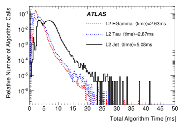
Figure 29: Execution times per RoI for calorimeter clustering algorithms at (a) L2 and (b) EF. The mean execution time for each algorithm is given in the legend

Figure 29 shows the processing time per RoI for the EF e/gamma, tau, jet and $E_{\mathrm{T}}^{\mathrm{miss}}$ clustering algorithms. Since more complex offline algorithms are used at the EF, the processing times are longer and the distributions have more features than for L2. The mean execution times do not show the same dependence on RoI size as at L2, since algorithm differences are more significant than RoI size at the EF. The multiple peaks due to caching of data preparation results are clearly visible. The measured L2 and EF algorithm times are well within the requirements given in Section 2.

5.4 Muon Tracking

Muons are triggered in the ATLAS experiment within a rapidity range of $|\eta|<2.4$ DetectorPaper . In addition to the L1 trigger chambers (RPC and TGC), the HLT makes use of information from the MDT chambers, which provide precision hits in the $\eta$ coordinate. The CSC, that form the innermost muon layer in the region $2<|\eta|<2.7$, were not used in the HLT during 2010 data-taking period, but will be used in 2011.

5.4.1 Muon Tracking Algorithms

The HLT includes L2 muon algorithms that are specifically designed to be fast and EF algorithms that rely on offline muon reconstruction software CSCBook .

At L2, each L1 muon candidate is refined by including the precision data from the MDTs in the RoI defined by the L1 candidate. There are three algorithms used sequentially at L2, each building on the results of the previous step.

•

L2 MS-only: The MS-only algorithm uses only the Muon Spectrometer information. The algorithm uses L1 trigger chamber hits to define the trajectory of the L1 muon and opens a narrow road around this to select MDT hits. A track fit is then performed using the MDT drift times and positions and a $p_{\mathrm{T}}$ measurement is assigned using look-up tables.

•

L2 Muon Combined: This algorithm combines the MS-only tracks with tracks reconstructed in the inner detector (Section 5.1) to form a muon candidate with refined track parameter resolution.

•

L2 Isolated Muon: The isolated muon algorithm starts from the result of the combined algorithm and incorporates tracking and calorimetric information to find isolated muon candidates. The algorithm sums the $|p_{\mathrm{T}}|$ of inner detector tracks and evaluates the electromagnetic and hadronic energy deposits, as measured by the calorimeters, in cones centred around the muon direction. For the calorimeter, two different concentric cones are defined: an internal cone chosen to contain the energy deposited by the muon itself; and an external cone, containing energy from detector noise and other particles.

At the EF, the muon reconstruction starts from the RoI identified by L1 and L2, reconstructing segments and tracks using information from the trigger and precision chambers. There are three different reconstruction strategies used in the EF:

•

EF MS-only: Tracks are reconstructed using Muon Spectrometer information and extrapolated to determine track parameters at the interaction point and form MS-only muon candidates.

•

EF Combined: Using an outside-in strategy, MS-only muon candidates are combined with inner detector tracks to form combined muon candidates.

•

EF Inside-Out: The inside-out strategy starts with inner detector tracks and extrapolates them to the Muon Spectrometer to search for MS-only candidates in order to form combined muon candidates.

EF Combined and Inside-out are both used for the trigger and offline reconstruction; MS-only is an alternative strategy for specialized triggers. For the EF MS-only and EF Combined strategies, the reconstruction is performed in the following steps:

•

SegmentFinder: Segments are formed from hits in the trigger and precision chambers within each of the three layers of the muon detector.

•

TrackBuilder: The segments are combined to form tracks.

•

Extrapolator: The tracks are extrapolated to the interaction point, track parameters are corrected for energy loss in the traversed material, producing EF MS-only muon candidates.

•

Combiner: The tracks from the muon spectrometer are combined with inner detector tracks to form combined tracks, resulting in EF Combined muon candidates.

5.4.2 Muon Tracking Performance

Comparisons between online and offline muon track parameters are presented in this section; muon trigger efficiencies are presented in Section 6.3. Distributions of the residuals between online and offline track parameters ($\frac{1}{p_{\mathrm{T}}}$, $\eta$ and $\phi$) were constructed in bins of $p_{\mathrm{T}}$ and Gaussian fits were performed to extract the widths, $\sigma$, of the residual distributions as a function of $p_{\mathrm{T}}$. The inverse-$p_{\mathrm{T}}$ residual widths, $\sigma((\frac{1}{p_{\mathrm{T}}})^{\mathrm{trigger}}-(\frac{1}{p_{\mathrm{T}}})^{\mathrm{offline}})$, are shown in Fig. 30 as a function of the offline muon $p_{\mathrm{T}}$ for the L2 Muon Combined, EF MS-only and EF Combined reconstruction. As a consequence of the optimisations made for algorithm speed, the L2 has worse track parameter resolution than the EF. The increase in the L2 inverse-$p_{\mathrm{T}}$ widths at high $p_{\mathrm{T}}$ is due to the finite granularity of the look-up table used in the L2 MS-only algorithm; at lower values of $p_{\mathrm{T}}$ the inner detector $p_{\mathrm{T}}$ resolution dominates. The improvement in $p_{\mathrm{T}}$ resolution, particularly at lower $p_{\mathrm{T}}$  resulting from the inclusion of inner detector information is also evident from a comparison of the $p_{\mathrm{T}}$ resolution of the EF MS-only and combined algorithms. The $\eta$ residual widths, $\sigma(\eta^{tr}-\eta^{off})$, and $\phi$ residual widths, $\sigma(\eta^{tr}-\eta^{off})$, are shown as a function of $p_{\mathrm{T}}$ in Fig. 31 and Fig. 31 respectively. These figures show the residual widths for L2 and EF combined reconstruction and illustrate the good agreement between track parameters calculated online and offline.

Figure 30: Inverse-$p_{\mathrm{T}}$ residual widths as a function of offline muon $p_{\mathrm{T}}$ ($p_{\mathrm{T}}>13{\mathrm{\ Ge\kern-1.00006ptV}}$) for the L2 combined, EF MS-only and EF Combined reconstruction

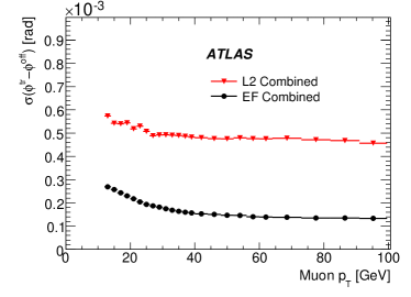
Figure 31: Residual widths as a function of the offline muon $p_{\mathrm{T}}$ ($p_{\mathrm{T}}>13{\mathrm{\ Ge\kern-1.00006ptV}}$) for 31 $\eta$ and 31 $\phi$ calculated by L2 and EF Muon Combined algorithms

Figure 32: Measured execution times per RoI for the 32 L2 MS-only algorithm and L2 Combined chain and 32 EF SegmentFinder, TrackBuilder, Extrapolator and Combiner algorithms. The mean time of each algorithm is indicated in the legend

5.4.3 Muon Tracking Timing

The processing times for the L2 muon reconstruction algorithms are shown in Fig. 32 for the MS-only algorithm and for the combined reconstruction chain, which includes the ID track reconstruction time. Figure 32 shows the corresponding times for the EF algorithms. The execution times are measured for each invocation of the algorithm, and are well within the time restrictions for both L2 and EF given in Section 2.

6 Trigger Signature Performance

In this section the different trigger signature selection criteria are described. The principal triggers used in 2010 are listed, their performance is presented and compared with Monte Carlo simulation and some references are given as examples of published results that rely on these triggers.

Efficiencies have been measured using the followingmethods:

•

Tag and probe method, where the event contains a pair of related objects reconstructed offline, such as electrons from a $Z\rightarrow ee$ decay, one that triggered the event and the other that can be used to measure trigger efficiency;

•

Orthogonal triggers method, where the event is triggered by a different and independent trigger from the one for which the efficiency is being determined;

•

Bootstrap method, where the efficiency of a higher threshold is determined using a lower threshold to trigger the event.

An example of the tag and probe method is the determination of low-$p_{\mathrm{T}}$ muon trigger efficiencies using $J/\psi\rightarrow\mathrm{\mu\mu}$ events. In this method, $\mathrm{\mu\mu}$ pairs are selected from $J/\psi\rightarrow\mathrm{\mu\mu}$ decays reconstructed offline in events triggered by a single muon trigger. The tag is selected by matching (in $\Delta R$) one of the offline muons with a trigger muon that passed the trigger selection. The other muon in the $\mathrm{\mu\mu}$ pair is defined as the probe. The efficiency is then defined as the fraction of probe muons that match (in $\Delta R$) a trigger muon that passes the trigger selection. An efficiency determined in this way must be corrected for background due to fake $J/\psi\rightarrow\mathrm{\mu\mu}$ decays reconstructed offline. The background subtraction uses a variable that discriminates the signal from the background, in this case, the invariant mass of $\mathrm{\mu\mu}$ candidates. By fitting this variable with an exponential background shape in the side bands and with a Gaussian signal shape in the $J/\psi$ mass region, the background content in the $J/\psi$ mass region can be determined and subtracted. The subtracted distribution is then used to determine the trigger efficiency. Biases due to, for example, topological correlations, are determined by MC.

6.1 Minimum Bias, High Multiplicity and Luminosity Triggers

Triggers were designed for inclusive inelastic event selection with minimal bias, for use in inclusive physics studies as well as luminosity measurements. Events selected by the minimum bias (minbias) trigger are used directly for physics analyses of inelastic $pp$ interactions Atlas:UE ; Atlas:ChargedPartMult , $PbPb$ interactions Atlas:DiJetAsymHI2010 , as well as indirectly as control samples for other physics analyses. A high multiplicity trigger is also implemented for studies of two-particle correlations in high-multiplicity events.

6.1.1 Reconstruction and Selection Criteria

The minbias and luminosity triggers are primarily hardware-based L1 triggers, defined using signals from the Minimum Bias Trigger Scintillators (MBTS), a Cherenkov light detector (LUCID), the Zero Degree Calorimeter (ZDC), and the random clock from the CTP. In addition to these L1 triggers, HLT algorithms are defined using inner detector and MBTS information (Section 2).

In 2010, inelastic $pp$ events were primarily selected with the L1_MBTS_1 trigger requirement, defined as having at least one of the 32 MBTS counters on either side of the detector above threshold. Several supporting MBTS requirements were also defined in case of higher beam-induced backgrounds and for online luminosity measurements. For some of these triggers (e.g. L1_MBTS_1_1) a coincidence was required between the signals from the counters on either side of the detector. In all cases, a coincidence with colliding bunches was required. During the $PbPb$ running the beam backgrounds were found to be significantly higher and selections requiring more MBTS counters above threshold on both sides of the detector were used.

The mbSpTrk trigger Atlas:minbCONFnote , used for minbias trigger efficiency measurements, selects events using the random clock of the CTP at L1 and inner detector tracker silicon space-points (Section 5.1) at the HLT.

The LUCID triggers were used to select events for comparison with real-time luminosity measurements. LUCID trigger items required a LUCID signal above threshold on one side , either side, or both sides of the detector. In all cases a coincidence with colliding proton bunches was required.

The ZDC detector was included in the ATLAS experiment primarily for selection of $PbPb$ interactions with minimal bias. Due to the ejection of neutrons from colliding ions, the ZDC covers most of the inelastic $PbPb$ cross-section, but not the inelastic $pp$ cross-section. Like the LUCID triggers, the ZDC triggers included a one-sided, either side, and two-sided trigger.

The high multiplicity trigger was based on a L1 total energy trigger and includes requirements on the number of L2 SCT space-points and the number of EF inner detector tracks associated to a single vertex.

The Beam Conditions Monitor (BCM) detectors were used to trigger on events with higher than nominal beam background conditions and were also used to monitor the luminosity.

6.1.2 Menu and Rates

The main minbias, high multiplicity and luminosity triggers used in the 2010 run are shown in Table 6. These triggers were prescaled for the majority of the 2010 data-taking to keep the rates around a few Hz.

Table 6: Minimum bias, high multiplicity and luminosity trigger items defined during the 2010 $pp$ and $PbPb$ running periods. In all cases, a filled bunch crossing is also required

	Trigger item	Definition
minbias triggers:	L1_MBTS_1(2)	$\geq$1(2) of the 2$\times$32 counters above threshold
	L1_MBTS_1_1	$\geq$1 counter above threshold in each side, in coincidence
	L1_MBTS_4_4	$\geq$4 counters above threshold in each side, in coincidence
	mbSpTrk	Random L1 trigger and space-points in the ID at HLT
luminosity triggers:	L1_LUCID_A(C)	At least one A(C)-side signal above threshold
	L1_LUCID_A_C	$\geq$1 signal above threshold in each side, in coincidence
	L1_LUCID	$\geq$1 signal above threshold
	L1_ZDC_A(C)	$\geq$1 A(C)-side signal above threshold
	L1_ZDC_A_C	$\geq$1 signal above threshold in each side, in coincidence
	L1_ZDC	$\geq$1 signal above threshold
high luminosity trigger:	mbSpTrkVtxMh	High Multiplicity trigger starting from L1_TE20

6.1.3 Minimum Bias Trigger Efficiency

The efficiency of the L1_MBTS_1 trigger was studied in the context of the charged particle multiplicity analysis Atlas:ChargedPartMult which used the L1_MBTS_1 trigger to select its dataset. The efficiency of the L1_MBTS_1 trigger was determined using the mbSpTrk trigger as an orthogonal trigger. The efficiency was defined as the fraction of events triggered by mbSpTrk passing the offline selection of an inelastic $pp$ interaction that also passed the L1_MBTS_1 trigger. This efficiency was determined with respect to offline-selected events containing at least two good tracks with $p_{\mathrm{T}}>100{\mathrm{\ Me\kern-1.00006ptV}}$, $|\eta|<2.5$, and transverse impact parameter with respect to the beamspot satisfying $d_{0}^{BS}<1.8$ mm. Events with more than one interaction were vetoed.

Figure 33 shows the L1_MBTS_1 efficiency as a function of the number of selected offline tracks per event, $N_{\mathrm{Track}}$, in the data sample. The inefficiency in the low $N_{\mathrm{Track}}$ region is small but visible.

Figure 33: The L1_MBTS_1 trigger efficiency for inelastic $pp$ collisions at $\sqrt{s}={7}{\mathrm{\ Te\kern-1.00006ptV}}$. The shaded areas represent the statistical and systematic uncertainties added in quadrature. The statistical uncertainty is negligible compared to the systematic uncertainty

One source of systematic uncertainty in the measured efficiency is a possible correlation between the control trigger (mbSpTrk) and L1_MBTS_1. The trigger efficiency of L1_MBTS_1 in the MC inelastic sample was calculated with and without the control trigger. The difference was found to be negligible. A second source investigated was the different impact parameter requirements from those in the offline selection. The trigger efficiency was studied with various sets of these requirements and the largest difference among these sets in each bin was taken as the systematic uncertainty for that bin. This variation provides a very conservative estimate of the effect of beam-induced background and secondary tracks on the trigger efficiency.

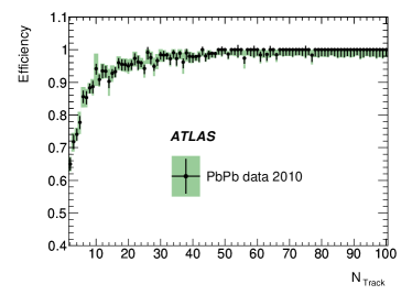
Figure 34: The L1_ZDC_A_C trigger efficiency as a function of the number of tracks for inelastic $PbPb$ collisions at $\sqrt{s_{NN}}=2.76{\mathrm{\ Te\kern-1.00006ptV}}$. The vertical bars represent the statistical uncertainty, while the shaded areas represent the statistical and systematic uncertainties added in quadrature

The efficiency of the ZDC trigger was measured in $PbPb$ collisions using a procedure similar to that used for the initial L1_MBTS_1 efficiency measurement. The efficiency is shown as a function of the number of tracks in the event in Fig. 34.

6.2 Electrons and Photons

Events with electrons and photons ($e/\gamma$) in the final state are important signatures for many ATLAS physics analyses, from SM precision physics, such as top quark or $W$ boson mass measurement, to searches for new physics. Various triggers cover the energy range between a few GeV and several TeV. In the low-$E_{\mathrm{T}}$ range (5-15 GeV), the data collected are used for measuring the cross sections and properties of standard candle processes, such as $J/\psi\rightarrow$ee, di-photon, low mass Drell-Yan, and $Z\rightarrow\tau\tau$ production. The data collected in the higher $E_{\mathrm{T}}$ range ($>15{\mathrm{\ Ge\kern-1.00006ptV}}$) are used to measure the production cross-sections for top quark pairs, direct photons and for the $Z\rightarrow ee$ and $W\rightarrow e\nu$ channels Atlas:WZleptons ; Atlas:topCS2010 ; InclPromptPhotonPaper ; Atlas:Wjets2010 , as well as searches for new physics such as Higgs bosons, SUSY and exotic particles as in extra-dimension models Atlas:diphotonMet2010 ; Atlas:susyOneLepton2011 . Some of these channels, such as $J/\psi\rightarrow$ee, $Z\rightarrow ee$, $W\rightarrow e\nu$ and $\gamma$+jet, are valuable benchmarks to extract the calibration and alignment constants, and to establish the detector performance.

6.2.1 Electron and Photon Reconstruction and Selection Criteria

Electrons and photons are reconstructed in the trigger system in the region $|\eta|<2.5$. At L1, photons and electrons are selected using calorimeter information with reduced granularity. For each identified electromagnetic object, RoIs are formed containing the $\eta$ and $\phi$ directions and the transverse energy thresholds that have been passed, e.g. EM5, EM10, as specified by the L1 trigger menu (Table 1). Seeded by the position of the L1 cluster, the L2 photon and electron selections employ a fast calorimeter reconstruction algorithm (Section 5.3), and in the case of electrons also fast track reconstruction (Section 5.1). The EF also performs calorimeter cluster and track reconstruction, but uses the offline reconstruction algorithms CSCBook .

At L2 and the EF a calorimeter-based selection is made, for both electrons and photons, based on cluster $E_{\mathrm{T}}$ and cluster shape parameters. Distributions of two important parameters are shown in Fig. 35. The hadronic leakage parameter, $R_{had}=E^{had}_{\textrm{T}}/E^{EM}_{\textrm{T}}$, is the ratio of the cluster transverse energy in the hadronic calorimeter to that in the electromagnetic calorimeter; the distribution for offline reconstructed electrons is shown in Fig. 35 for L2. Figure 35 shows the distribution, at the EF, of the parameter $E_{ratio}=(E_{T}^{(1)}-E_{T}^{(2)})/(E_{T}^{(1)}+E_{T}^{(2)})$ where $E_{T}^{(1)}$ and $E_{T}^{(2)}$ are the transverse energies of the two most energetic cells in the first layer of the electromagnetic calorimeter in a region of $\Delta\eta\times\texttimes\Delta\phi=0.125\times 0.2$. The distribution of this parameter peaks at one for showers with no substructure and so distinguishes clusters due to single electrons and photons from hadrons and $\pi^{0}\rightarrow\gamma\gamma$ decays. Another important parameter, $R_{\eta}$, is based on the cluster shape in the second layer of the electromagnetic calorimeter; it is defined as the ratio of transverse energy in a core region of $3\times 7$ cells in $\eta\times\phi$ to that in a $7\times 7$ region, expanded in $\eta$ from the $3\times 7$ core. In addition, the electron selection requires that a track be matched to the calorimeter cluster.

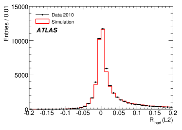
Figure 35: Distributions of the $e/\gamma$ cluster shape variables 35 $R_{had}$ at L2 and 35 $E_{ratio}$ at the EF for offline electrons passing the L1 EM trigger with a nominal 3 GeV threshold

For electrons, three sets of reference cuts are defined with increasing power to reject background: loose, medium, and tight. All selections include the same cuts on the shower shape parameter, $R_{\eta}$, and hadronic leakage parameter, $R_{had}$. The medium selection adds cuts on the shower shape in the first calorimeter layer, $E_{ratio}$, track quality requirements and stricter cluster-track matching.The tight selection adds, on top of the medium selection, requirements on the ratio, $E_{T}/p_{T}$, of calorimeter cluster $E_{T}$ to inner detector track $p_{T}$, a requirement for a hit on the innermost tracking layer, and particle identification by the TRT.

For photons, two reference sets of cuts, loose and tight, are defined. Only the loose selections were used for triggering in 2010. The loose photon selection is the same as the calorimeter-based part of the loose electron selection. The tight selection, in addition, applies cuts on cluster shape in the first calorimeter layer, $E_{ratio}$, and further requirements on cluster shape in the second calorimeter layer. For more detailed information on $e/\gamma$ triggers in 2010, see Ref. Atlas:egammaCONFnote .

Table 7: Principal $e/\gamma$ triggers and approximate HLT rates at a luminosity of $10^{32}\,\text{cm}^{-2}\text{s}^{-1}$. The rates given are inclusive; there are significant overlaps between triggers

Trigger	Motivation	Rate [Hz]
2e5_tight	$J/\psi\rightarrow$ee, Drell-Yan	1
2e10_loose	$Z\rightarrow ee$, Drell-Yan	1
e10_loose_mu6	SM physics, di-lepton searches e.g. for Higgs searches	1
2g15_loose	di-photon cross-section, di-photon searches	1
e15_medium	high-$p_{\mathrm{T}}$ physics	20
e20_loose	high-$p_{\mathrm{T}}$ physics	22
g40_loose	direct photons and searches for new particles	5

6.2.2 Electron and Photon Trigger Menu and Rates

Table 7 gives an overview of the rates of the main $e/\gamma$ triggers used in the 2010 menu for instantaneous luminosities around $10^{32}\,\text{cm}^{-2}\text{s}^{-1}$. The $E_{\mathrm{T}}$ thresholds of the electron and photon triggers range from $5{\mathrm{\ Ge\kern-1.00006ptV}}$ to $40{\mathrm{\ Ge\kern-1.00006ptV}}$. In addition, supporting triggers were deployed, which were used for efficiency extraction, monitoring, commissioning and cross-checks. The overall rate of the $e/\gamma$ trigger stream was $\sim$70 Hz at $\mathcal{L}$=$10^{32}\,\text{cm}^{-2}\text{s}^{-1}$, constituting $\sim$25% of the total bandwidth written to mass storage at the end of 2010.

The L1 and HLT trigger rates of $e/\gamma$ triggers are shown in Fig. 36 as a function of luminosity. No significant deviation from linearity was observed during 2010 running. It should be noted that during the course of 2010, no deterioration in performance of $e/\gamma$ triggers or effect on rates was observed due to in-time or out-of-time pile-up.

Figure 36: Observed rates for primary $e/\gamma$ triggers at (a) L1, before pre-scaling (PS), and (b) EF, after pre-scaling

6.2.3 Electron and Photon Trigger Efficiencies

Trigger efficiencies are presented for electrons and photons identified by the offline reconstruction. More details are given in Ref. Atlas:egammaCONFnote , including a full study of the systematic uncertainties in the plateau efficiencies which amount to $\sim$ 0.4% for the electron trigger and  $\sim$ 1% for the photon trigger. The EF selection of electrons and photons is very similar to the offline identification: the same criteria are used for loose, medium and tight selections in offline reconstruction as detailed in Section 6.2.1.

The determination of the efficiencies of electron and photon triggers share the following common selection criteria. Collision event candidates are selected by requiring a primary vertex with at least three tracks. Rare events that contain very localised high-energy calorimeter deposits not originating from proton-proton collisions, for example from sporadic discharges in the calorimeter or cosmic ray muons undergoing a hard bremsstrahlung, are removed, resulting in predicted losses of less than 0.1% of minimum-bias events and 0.004% of $W\rightarrow e\nu$ events WinclPaper . In addition, events are rejected if the candidate electromagnetic cluster is located in a problematic region of the EM calorimeter, for example where the effect of inactive cells could be significant. Due to hardware problems LArPaper , the signal could not be read out from $\sim$2% of the EM calorimeter cells in 2010. Offline electrons are selected if they are within the region $|\eta|<2.47$ and outside the transition between the barrel and end-caps of the EM calorimeter, $1.37<|\eta|<1.52$. The acceptance region for photons is limited to $|\eta|<2.37$ due to the geometrical acceptance of the first layer of the EM calorimeter (fine strips in the $\eta$ direction), which is crucial for the rejection of background photons originating from $\pi^{0}$ decay.

The decays $Z\rightarrow ee$ and $W\rightarrow e\nu$ provide samples to measure the electron trigger efficiency in the higher-$E_{\mathrm{T}}$ range ($>15{\mathrm{\ Ge\kern-1.00006ptV}}$). The $Z\rightarrow ee$ decays provide a sample of electrons to use with the tag-and-probe method. In the case of $W\rightarrow e\nu$ decays, the orthogonal trigger method is employed, using the $E_{\mathrm{T}}^{\mathrm{miss}}$ triggers with thresholds between 20 and $40{\mathrm{\ Ge\kern-1.00006ptV}}$ to collect the data sample. Figure 37 compares the efficiencies of the e15_medium and e20_loose triggers at the EF, measured in $W$ boson events with those measured in $Z$ boson events. The efficiencies are measured with respect to offline tight electrons as functions of the offline electron $E_{\mathrm{T}}$ and $\eta$. The efficiencies measured by the two methods are in excellent agreement, differing by less than about 1%. The dominant contribution (0.4%) to the systematic uncertainty in the plateau efficiency comes from an analysis of the spread of differences in efficiency between data and simulation as a function of $E_{\mathrm{T}}$ and $\eta$. Figure 37 shows that the response in $\eta$ is flat except at the outer edges of the end-caps. Above $20{\mathrm{\ Ge\kern-1.00006ptV}}$ the e15_medium trigger efficiency for $W\rightarrow e\nu$ and $Z\rightarrow ee$ events is greater than 99%.

Figure 37: Efficiencies for the e15_medium and e20_loose triggers, measured with respect to offline tight electrons in $W\rightarrow e\nu$ and $Z\rightarrow ee$ events, shown as a function of 37 $E_{\mathrm{T}}$ and 37 $\eta$

In contrast to electrons, there is no suitable decay channel that would allow the trigger efficiency to be measured for prompt photons in the $\sim 10-50{\mathrm{\ Ge\kern-1.00006ptV}}$ energy range using tag and probe or orthogonal triggers. Therefore, the bootstrap method is used, where the HLT efficiency is measured for events that pass a lower L1 $E_{\mathrm{T}}$ threshold. For example, the g20_loose efficiency is measured using a sample of events passing the $14{\mathrm{\ Ge\kern-1.00006ptV}}$ $E_{\mathrm{T}}$ L1 threshold (EM14). In most physics analyses, the photons are selected offline with tight identification requirements. Thus, the trigger efficiency is shown with respect to photons identified with the tight offline requirements. The bootstrap method relies on measuring the HLT efficiency in a $p_{\mathrm{T}}$ region where the L1 trigger is fully efficient with respect to offline photons. It has been verified that L1_EM14 is fully efficient for photon clusters with $E_{\mathrm{T}}>20{\mathrm{\ Ge\kern-1.00006ptV}}$ using a sample of events selected by the L1_EM5 trigger. The bootstrap method suffers from a large contamination of fake photons, such as hadronic jet clusters mis-reconstructed as photons. The bias on the measured efficiency has been estimated to be less than $\sim$0.25% for photons with $E_{\mathrm{T}}>~{}25$ GeV by comparing the efficiencies from data with those from a signal-only simulation. Figure 38 shows the L2 and EF efficiencies for the g20_loose trigger, as functions of offline tight photon $E_{\mathrm{T}}$ and $\eta$. For the $\eta$ distribution, photons were selected with $E_{\mathrm{T}}>25{\mathrm{\ Ge\kern-1.00006ptV}}$ in the plateau region of the turn-on curve.

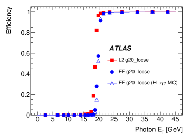
Figure 38: Photon efficiencies measured with the bootstrap method, as a function of the offline tight photon 38 $E_{\mathrm{T}}$ and 38 $\eta$ (with $E_{\mathrm{T}}>25{\mathrm{\ Ge\kern-1.00006ptV}}$) for events passing the L1_EM14 threshold

Table 8: Principal muon triggers and their approximate HLT rates at a luminosity of $10^{32}\,\text{cm}^{-2}\text{s}^{-1}$

Trigger	Motivation	Rate [Hz]
mu13	$Z\rightarrow\mu\mu$, $W\rightarrow\mu\nu$, top, new physics	12
mu40_MSonly	new physics	20
2mu6	$Z\rightarrow\mu\mu$, Drell-Yan, $B$ physics, new physics	14

The L2 and EF g20_loose triggers reach the efficiency plateau at about $E_{\mathrm{T}}=25{\mathrm{\ Ge\kern-1.00006ptV}}$, with efficiencies above this threshold of greater than 99% for both L2 and EF. The efficiency remains flat, at the plateau value, as far as can be tested in the 2010 data, up to $\sim 500{\mathrm{\ Ge\kern-1.00006ptV}}$. The agreement between the efficiencies measured in data and simulated events is better than 1%.

6.3 Muons

Muons are produced in many final states of interest to the broad physics programme being conducted at the LHC, from SM precision physics, such as top quark and $W$ boson mass measurements, to searches for new physics. Muons are identified with high purity compared to other signatures and cover a wide momentum range between a few GeV and several TeV. Trigger thresholds in the $p_{\mathrm{T}}$ range $4-10{\mathrm{\ Ge\kern-1.00006ptV}}$ are used to collect data for measurements of processes such as $J/\psi\rightarrow\mathrm{\mu\mu}$, low-$p_{\mathrm{T}}$ di-muons, and $Z\rightarrow\tau\tau$. Higher $p_{\mathrm{T}}$ thresholds are used to collect data used to measure the properties of SM particles such as $W$and $Z$ bosons, and top quarks, Atlas:WZleptons ; Atlas:topCS2010 ; Atlas:Wjets2010 as well as to search for new physics, like the Higgs boson, SUSY Atlas:susyOneLepton2011 and extra-dimension models. Some of these channels, such as $J/\psi\rightarrow\mathrm{\mu\mu}$, $Z\rightarrow\mu\mu$, and $W\rightarrow\mu\nu$ decays are valuable benchmarks to extract calibration and alignment constants, and to establish the detector performance.

6.3.1 Muon Reconstruction and Selection Criteria

The trigger reconstruction algorithms for muons at L1 and the HLT are described in Sections 4.3 and 5.4 respectively. The selection criteria applied to reconstructed muon candidates depend on the algorithm with which they were reconstructed. The MS-only algorithm selects solely on the $p_{\mathrm{T}}$ of the muon; the combined algorithm makes selections based on the match between the inner detector and muon spectrometer tracks and their combined $p_{\mathrm{T}}$; the isolated muon algorithm applies selection criteria based on the amounts of energy found in the isolation cones.

6.3.2 Muon Trigger Menu and Rates

Table 8 gives an overview of the principal muon triggers and their approximate rates at a luminosity of $10^{32}\,\text{cm}^{-2}\text{s}^{-1}$. In addition to these principal physics triggers, a range of supporting triggers were included for commissioning, monitoring, and efficiency measurements. In 2010 running, in order to maximize acceptance, all HLT selections were based on L1 triggers using the low-$p_{\mathrm{T}}$ logic (described in Section 4.3), including mu13, mu20 and mu40 that were seeded from the L1 MU10 trigger.

Figure 39: Observed mean trigger rates as a function of the instantaneous luminosity for 39 L1 and 39 the EF

The trigger rates at L1, L2, and EF are dependent on thresholds, algorithms (Section 5.4) and luminosity. The trigger rates have been measured as a function of the luminosity and parametrized with Equation (1):

$$r=c_{1}\mathcal{L}+c_{0}N_{BC},$$ (1)

where $r$ is the rate, $\mathcal{L}$ the instantaneous luminosity, $N_{BC}$ the number of colliding bunches, and $c_{1}$, $c_{0}$ are proportionality constants. The second term represents the contribution to the trigger rate from cosmic rays: as the number of colliding bunches increases, so does the amount of time the trigger gate is open to accept cosmic rays. The instantaneous luminosity was taken from the online measurements averaged over ten successive luminosity blocks.

The measured muon trigger rates are shown for L1 and EF in Fig. 39 together with lines representing the result of fitting Equation (1) to the measurements. Steps in the rate are due to the increases in $N_{BC}$, and hence the contribution to the rate from cosmic rays. This is significant at L1 and for algorithms using only the muon spectrometer data at the HLT. For combined algorithms, the contribution from cosmic rays to the rate is negligible (within the errors of the fit).

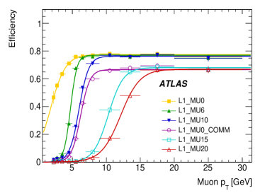
Figure 40: L1 trigger efficiency for combined muons reconstructed offline for 40 RPC and 40 TGC triggers. A Fermi function is fitted to the measurements for each trigger. Statistical uncertainties are represented by vertical bars

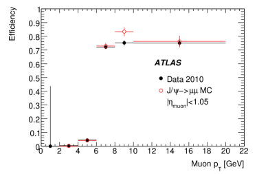
Figure 41: Efficiencies of the 6 GeV threshold combined muon trigger (mu6) as a function of reconstructed muon $p_{\mathrm{T}}$ for $J/\psi\rightarrow\mathrm{\mu\mu}$ decays in data and simulation for the 41 barrel and 41 end-caps. Statistical uncertainties are represented by vertical bars

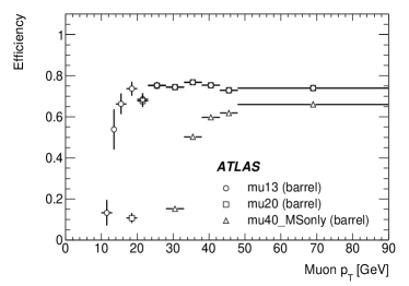
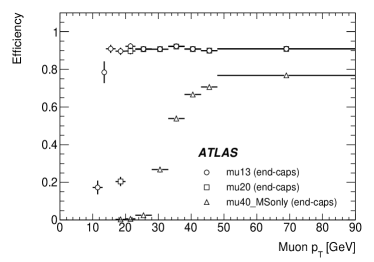
Figure 42: Efficiencies in the 42 barrel and 42 end-caps of the combined muon triggers with 13 GeV and 20 GeV thresholds and the MS-only trigger with a 40 GeV threshold. Statistical uncertainties are represented by vertical bars

6.3.3 Muon Trigger Efficiency

The muon trigger efficiencies have been measured for offline muons Atlas:muonCONFnote . The L1 RPC trigger efficiencies measured using an orthogonal L1 calorimeter trigger are shown in Fig. 40 for various thresholds. The efficiencies measured using the tag and probe method with $J/\psi\rightarrow\mathrm{\mu\mu}$ and $Z\rightarrow\mu\mu$ decays are shown for the L1 TGC trigger in Fig. 40. The geometrical acceptance of the RPC low-$p_{\mathrm{T}}$ trigger is about 80% which explains the lower efficiency compared to the TGC trigger, which has a geometrical acceptance close to 95%. For the RPC trigger, a further reduction in plateau efficiency is evident for the high-$p_{\mathrm{T}}$ ($p_{\mathrm{T}}>$10 GeV) triggers compared to the low-$p_{\mathrm{T}}$ triggers ($p_{\mathrm{T}}\leq$10 GeV). About half (6%) of this difference is due to a smaller geometrical coverage of the high-$p_{\mathrm{T}}$ triggers. Part of this inefficiency will be recuperated in the muon spectrometer upgrade planned for 2013. The remaining difference is largely due to detector inefficiency which affects the high-$p_{\mathrm{T}}$ trigger more than the low-$p_{\mathrm{T}}$ trigger due to the additional coincidence requirements. Improved efficiency is expected for 2011 running.

The efficiency in the HLT was determined using the tag and probe method with $J/\psi\rightarrow\mathrm{\mu\mu}$ samples for low $p_{\mathrm{T}}$ ($6{\mathrm{\ Ge\kern-1.00006ptV}}$) triggers and $Z\rightarrow\mu\mu$ for high $p_{\mathrm{T}}$ ($13{\mathrm{\ Ge\kern-1.00006ptV}}$) triggers. In both studies, collision events were selected by requiring that the event has at least three tracks associated with the same reconstructed primary vertex. Reference muons reconstructed offline using both ID and MS information were required to be inside the fiducial volume of the muon triggers ($|\eta|<2.4$) and the associated ID track was required to have at least one Pixel hit and at least six SCT hits. Events were required to contain a pair of reference muons with opposite charge and an invariant mass lying within a window around the mass of the relevant resonance:
$2.86{\mathrm{\ Ge\kern-1.00006ptV}}<m_{\mu\mu}<3.34{\mathrm{\ Ge\kern-1.00006ptV}}$ for $J/\psi\rightarrow\mathrm{\mu\mu}$ decays and $77{\mathrm{\ Ge\kern-1.00006ptV}}<m_{\mu\mu}<106{\mathrm{\ Ge\kern-1.00006ptV}}$ for $Z\rightarrow\mu\mu$ decays. The resulting efficiency in the low-$p_{\mathrm{T}}$ region for the mu6 trigger is shown in Fig. 41. For the high-$p_{\mathrm{T}}$ region, Fig. 42 shows the efficiency as a function of $p_{\mathrm{T}}$ for the mu13, mu20 and mu40_MSonly triggers in the TGC and RPC regions derived from the weighted average of the efficiency measured from the $J/\psi$ and $Z$ samples. Note that the 40 GeV threshold trigger has not yet reached its plateau efficiency in the highest $p_{\mathrm{T}}$ bin in the figure; extending the figure to higher $p_{\mathrm{T}}$ is limited by the small number of probe muons above 90GeV. The efficiencies are seen to have a sharp turn-on with a plateau efficiency ($p_{\mathrm{T}}>13$ GeV) for the mu13 trigger of 74% for the barrel region (dominated by the RPC geometrical acceptance), Fig. 42, and 91% for the end-cap region, Fig. 42. The systematic uncertainty on the plateau efficiency has been evaluated to be $\sim$1%.

Table 9: The primary triggers in each of the jet trigger categories with their L1 threshold and approximate prescale factor for an instantaneous luminosity of $\sim 10^{32}\,\text{cm}^{-2}\text{s}^{-1}$ (a prescale value of 1 means unprescaled). The trigger name contains the EF threshold value; the L2 threshold is 5 GeV lower

Category	Name	L1 Threshold	Prescale	Motivation
Inclusive Jets:	j20	J5	$\sim 10^{5}$	jets in central region ($|\eta|<3.2$)
	j30	J10	$\sim 10^{4}$
	j35	J15	$\sim 10^{4}$
	j50	J30	$\sim 10^{3}$
	j75	J55	$\sim 10^{2}$
	j95	J75	$\sim 10$
	none	J95	1
Forward Jets:	fj30	FJ10	$\sim 10^{3}$	jets in the forward region ($|\eta|>3.2$)
	fj50	FJ30	$\sim 50$
	fj75	FJ55	$\sim 10$
	none	FJ95	1
Multi-jets:	2j75	2J70	$\sim 30$	two or more central jets above threshold
	3j30	3J10	$\sim 200$
	4j30	4J10	$\sim 5$
	5j30	5J10	1
Total Jet $E_{\mathrm{T}}$:	je195	JE100	$\sim 70$	total $E_{\mathrm{T}}$ of all jets above threshold
	je255	JE140	1

6.4 Jets

Jet signatures are important for QCD measurements Atlas:JetDiJetInc2010 ; Atlas:JetShapes2010 , top quark measurements, and searches for new particles decaying into jets Atlas:diJetSearch2010 ; Atlas:ContIntSearch2010 . Data collected with jet triggers also provide important control samples for many other physics analyses. Jet triggers select events containing high $p_{\mathrm{T}}$ clusters, and can be separated into four categories: inclusive jets (J), forward jets (FJ), multi-jets (nJ, n=2,3..), and total jet $E_{\mathrm{T}}$ (JE).

6.4.1 Jet Reconstruction and Selection Criteria

For a large part of 2010 data-taking, only L1 jet triggers (Section 4.2) were used for selection. L2 rejection was enabled late in 2010, while EF rejection was not enabled during 2010 running as it was not needed Atlas:jetCONFnote .

Calibration constants that correct for the hadron response of the non-compensating calorimeters in ATLAS (hadronic energy scale) were not applied in the trigger during 2010 data-taking. As a result, the jet trigger algorithms applied cuts to energy variables at the electromagnetic scale, the scale for energy deposited by electrons and photons in the calorimeter.

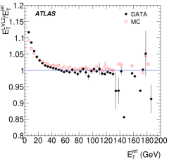
Figure 43: Ratios of transverse momenta of jets in $|\eta|<2.8$ reconstructed at L2 and jets reconstructed offline with the anti-$k_{\mathrm{T}}$ algorithm with parameter $R=0.4$, as a function of the offline jet $E_{\mathrm{T}}$. For this comparison, both online and offline jet energies have been calibrated to the electromagnetic energy scale. The errors shown are statistical only

Figure 43 shows the ratio of the L2 jet $E_{\mathrm{T}}$ to the offline jet $E_{\mathrm{T}}$  as a function of the offline jet $E_{\mathrm{T}}$. Data and MC simulation agree well.

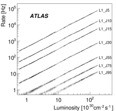
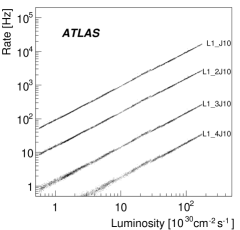
Figure 44: Rates for various L1 jet triggers as a function of the instantaneous luminosity during the 2010 run for 44 inclusive triggers and 44 multi-jet triggers (with the inclusive trigger L1_J10 for reference)

6.4.2 Jet Trigger Menu and Rates

The principal jet triggers for an instantaneous luminosity of $\sim 10^{32}\,\text{cm}^{-2}\text{s}^{-1}$ are listed in Table 9 for inclusive jets, forward jets, multi-jets, and total jet $E_{\mathrm{T}}$. The set of L1 prescales applied provided an approximately flat event yield as a function of jet $p_{\mathrm{T}}$. The L1 rates of the inclusive and multi-jet triggers are shown in Fig. 44. During 2010 running, the level of pileup was small enough not to have a visible effect on the rates, which were observed to rise linearly with instantaneous luminosity.

6.4.3 Jet Trigger Efficiency

The jet trigger efficiency was measured using the orthogonal trigger and bootstrap methods. For the lowest-threshold chains, the jet trigger efficiency was calculated using the orthogonal trigger method with events selected by the L1_MBTS_1 trigger (Section 6.1). For the higher thresholds, the bootstrap method was used. The systematic uncertainty in the plateau efficiencies is less than $\sim$1%.

This efficiency determination Atlas:JetDiJetInc2010 used jets that were reconstructed offline from calorimeter clusters at the electromagnetic scale, using the anti-$k_{\mathrm{T}}$ jet algorithm antikt with $R=0.4$ or $R=0.6$, in the region $|\eta|<2.8$. These jets were calibrated for calorimeter response to hadrons using parameters taken from the simulation, after comparison with the data JES . Cleaning cuts were applied to suppress fake jets from noise, cosmic rays, and other sources. These cleaning cuts were designed to reject pathological jets with almost all energy coming from a very small number of cells, out-of-time cell signals, or abnormal electromagnetic components. These cuts are explained in detail in Ref. JetCleaning .

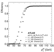
Figure 45: 45 Efficiency of the L1_J30 trigger as a function of offline jet transverse momentum (after applying hadronic calibration) for two different data-taking periods. For the second period the efficiency of the L2_j45 trigger is also shown. 45 Efficiency for several triggers, integrated over 2010

Figure 46: Efficiency for two L1 thresholds of the forward jet trigger

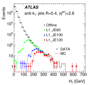
Figure 47: Offline transverse momentum distribution for all jets, and for those passing each of three thresholds of the L1 total jet $E_{\mathrm{T}}$ trigger

The efficiency of the L1_J30 jet trigger in the central region, $|\eta|<0.8$, of the detector is shown in Fig. 45 as a function of offline jet $p_{\mathrm{T}}$ for two different data-taking periods, the difference between the periods being that in periods G to I the LHC beam had a bunch train structure. The change in bunch structure had a small effect on the efficiency turn-on curve and a negligible effect on the efficiency in the plateau region. The efficiency of the L2_j45 trigger chain, which includes the L1_J30 trigger, is also shown in Fig. 45 for periods G to I, for which L2 rejection was enabled. Since the efficiency turn-on is significantly sharper for L2 than L1, the L2 thresholds were set 15 GeV higher than the L1 values, reducing the overall trigger rate while ensuring that the L2 trigger reached full efficiency at the same $p_{\mathrm{T}}$ value as the corresponding L1 trigger. Jet trigger efficiencies integrated over the whole year are shown in Fig. 45 for several chains as a function of the calibrated offline jet $p_{\mathrm{T}}$. Figure 46 shows the efficiency for two thresholds of the inclusive forward trigger. The efficiency plateaus at a lower $p_{\mathrm{T}}$ than for central jet triggers due to different energy resolutions and different contributions from noise and pile-up. After reaching the plateau, the jet and forward jet triggers remain fully efficient to within $\sim$1%.

The total jet $E_{\mathrm{T}}$ triggers require the $E_{\mathrm{T}}$ sum of all jets in the event (defined as $H_{\mathrm{T}}$) to be higher than a given threshold and have the effect of selecting events with high jet multiplicity. Figure 47 shows the distribution of $H_{\mathrm{T}}$ for events, triggered by an orthogonal muon trigger, that pass three different JE trigger thresholds, compared to predictions from the MC. The MC distributions are in agreement with the data.

Figure 48: The $\Delta\phi$ between the highest $p_{\mathrm{T}}$ and second highest $p_{\mathrm{T}}$ jet in the event for jets reconstructed at L2

In the initial phase of data-taking the jet triggers were limited to inclusive and multi-jet topologies, with no cuts on the relative directions of the jets. Near the end of the 2010 data-taking, additional triggers that require di-jets with large rapidity differences or small differences in azimuthal angle were implemented at L2. Figure 48 shows the $\Delta\phi$ distributions for di-jets at L2, indicating that these distributions are well described by the simulation.

6.5 Taus

The ATLAS physics programme uses tau leptons for SM measurements and new physics searches. Being able to trigger on hadronic tau signatures is important for this part of the ATLAS physics programme. Dedicated trigger algorithms have been designed and implemented based on the features of hadronic tau decays: narrow calorimeter clusters and a small number of associated tracks. Due to the high production rate of jets with very similar features to hadronic tau decays, keeping the rate of tau triggers under control is particularly challenging.

Figure 49: Comparison of (a) the variable $\Sigma p_{\mathrm{T}}^{\mathrm{iso}}/\Sigma p_{\mathrm{T}}^{\mathrm{core}}$ at L2 and (b) $\mathcal{R}_{\mathrm{EM}}$ at the EF in periods A-C (no pile-up) and period I (in-time pile-up of between two and three collisions per bunch crossing and 150 ns bunch trains)

6.5.1 Tau Reconstruction and selection criteria

At L1 the tau trigger uses EM and hadronic calorimeter information within regions of 4$\times$4 trigger towers ($\Delta\eta\times\Delta\phi\approx 0.4\times 0.4$) to calculate the energy in a core and an isolation region (Section 4.2).

At L2 selection criteria are applied using tracking and calorimeter information, taking advantage of narrowness and low track multiplicity to discriminate taus from jets. The L2 tau candidate is reconstructed from cells in a rectangular L2 RoI of size $\Delta\eta\times\Delta\phi=0.6\times 0.6$ centred at the L1 RoI position. The L2 calorimeter algorithm first refines the L1 RoI position using the second layer of the EM calorimeter. It then selects narrow jets in the detector by means of a calorimeter shape variable determined only from the second layer of the EM calorimeter. The shape variable, $\mathcal{R}_{EM}$, is an energy-weighted radius squared within the L2 RoI, i.e.

$$\mathcal{R}_{\mathrm{EM}}=\frac{\displaystyle\sum_{\mathrm{cell}}E_{\mathrm{cell}}\cdot(\Delta R_{\mathrm{cell}})^{n}}{\displaystyle\sum_{\mathrm{cell}}E_{\mathrm{cell}}}$$ (2)

where $E_{\mathrm{cell}}$ is the energy of the calorimeter cell and $\Delta R_{\mathrm{cell}}$ is the radius $\Delta R$ (defined in Section 5.1) of the cell from the centre of the L2 RoI, which is squared ($n=2$). Track reconstruction at L2 uses the SiTrack algorithm (Section 5.1), but to minimize the execution time, tracks are not extended to the TRT. Tracks with $p_{\mathrm{T}}>1.5$ GeV are reconstructed in the L2 RoI.

Exploiting the same characteristics of narrowness and low track multiplicity, the EF selects 1-prong and multi-prong decays, with different selection criteria, using algorithms that are similar to the offline reconstruction algorithms DetectorPaper . The EF tau candidate is reconstructed from cells in a rectangular region of size $\Delta\eta\times\Delta\phi=0.8\times 0.8$ centred at the L1 RoI position. The position, transverse energy, and calorimeter shower shape variables of the EF tau candidate are calculated from cells of all calorimeter layers within this $0.8\times 0.8$ region. An overall hadronic calibration JetCalibration is applied to all cells, and a tau-specific calibration is applied to the tau trigger candidate. The EM radius shape variable used at the EF is defined by Equation 2 with $n=1$. Additional quality criteria are applied to tracks reconstructed in the RoI, and if more than one track is found a secondary vertex reconstruction is attempted.

The stability of the tau trigger selection variables against pile-up was evaluated by comparing the distributions of these variables for events passing the L1_TAU5 trigger from data-taking periods A-C with those from period I. Periods A-C contain a negligible amount of pile-up, while events from period I contain the largest amount of pile-up (Section 2) observed in 2010. The distributions of the two most important variables ($\Sigma p_{\mathrm{T}}^{\mathrm{iso}}/\Sigma p_{\mathrm{T}}^{\mathrm{core}}$ at L2 and $\mathcal{R}_{\mathrm{EM}}$ at EF) are shown in Fig. 49 for events with and without pile-up. The variable $\Sigma p_{\mathrm{T}}^{\mathrm{iso}}/\Sigma p_{\mathrm{T}}^{\mathrm{core}}$ describes the ratio of the scalar $p_{\mathrm{T}}$ sums of the tracks in an isolation ring (R=0.1 to 0.3) and in the core area (R=0.1). The plots show a small shift due to the presence of additional energy and tracks, but these variables are in general quite stable with respect to the pile-up of two to three collisions per bunch crossing. The same behaviour was observed for other variables used for making the HLT decision.

Table 10: Tau trigger menu and approximate HLT rates for a luminosity of $10^{32}\,\text{cm}^{-2}\text{s}^{-1}$

Trigger	Motivation	Rate [Hz]
tau50_medium	$H^{+}$, $Z^{\prime}$	8
2tau29_loose1	$H$, $Z^{\prime}$	1
tau16_medium_xe22	$H^{+}$, $t$, $W$	10
tau12_loose_e10_medium	$H$, $t$, $Z$	4
tau12_loose_mu10	$H$, $t$, $Z$	3

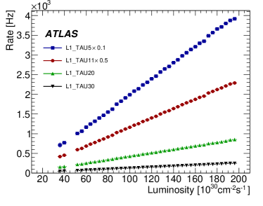
Figure 50: Trigger rates as a function of instantaneous luminosity for several (a) L1 and (b) HLT tau triggers. The rates for L1_TAU5 and L1_TAU11 have been scaled by 0.1 and 0.5 respectively

6.5.2 Tau Trigger Menu and Rates

Both single tau triggers and tau triggers in combination with electrons, muons, jets and missing energy signatures were present in the 2010 trigger menus. Tau signatures were used in combination with other triggers to keep rates low enough while maintaining acceptance for the physics processes of interest. Table 10 shows a subset of these items with their rates that represent the lowest threshold triggers that remained unprescaled at a luminosity of $10^{32}\,\text{cm}^{-2}\text{s}^{-1}$.

Figure 50 shows the trigger rates for various L1 and HLT tau triggers as a function of instantaneous luminosity showing a linear increase of rates during 2010 running.

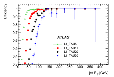
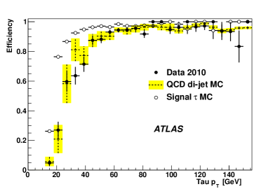
Figure 51: Efficiency for 51 jets reconstructed offline with at least one associated track to pass the L1 tau trigger with thresholds of 5, 11, 20 and $30{\mathrm{\ Ge\kern-1.00006ptV}}$ as a function of the offline jet $E_{\mathrm{T}}$ and 51 offline tau candidates to pass the HLT tau16_loose trigger in a di-jet data sample, simulated QCD di-jets and a simulated tau signal sample, as a function of the offline tau $p_{\mathrm{T}}$

6.5.3 Tau Trigger Efficiency

Tau trigger efficiencies were measured using offline reconstructed tau candidates in events containing QCD jets. Since QCD jets are the biggest source of fake taus in data, a sample of jets reconstructed offline provides a useful reference for tau trigger performance measurements. For the L1 trigger efficiency determination, offline jets were reconstructed with the anti-$k_{\mathrm{T}}$ algorithm (using parameter R = 0.4) and required to have at least one associated track. Figure 51 shows the efficiency of the L1_TAU trigger for these jets, as a function of the jet $E_{\mathrm{T}}$. Although the L1 trigger efficiency has a slower turn-on for jets than for true taus, due to the wider shower profile of QCD jets, above the turn-on region the performance is similar, as confirmed from MC simulation studies. The L1 trigger efficiency reaches a plateau value of 100% (to within a systematic uncertainty of $\sim$1%).

Figure 51 shows the efficiency of the tau16_loose trigger for offline tau candidates in data, simulated di-jet events, and simulated signal $\tau$ events. Data events were selected by requiring two back-to-back jets (within 0.3 radians), balanced in $p_{\mathrm{T}}$ (within 50% of the higher $p_{\mathrm{T}}$ jet). The data sample was collected with jet triggers (Section 6.4). Bias related to the jet trigger selection was removed by randomly selecting one of the jets (tag jet) that passed the jet trigger and using the other jet (probe jet) to match to a reconstructed tau candidate. Reconstructed tau candidates that pass the tight offline identification requirements and match a probe jet ($\Delta R<0.4$) were used as the denominator of the efficiency measurement. The numerator was defined as the subset of those candidates that also passed the tau16_loose trigger. The efficiencies from data agree with those for the simulated di-jets, but have a slower turn-on than for the simulated signal sample. This is because of the lower L1 efficiency for jets than taus in the threshold region. The trigger efficiency for offline tau candidates with $p_{\mathrm{T}}>30{\mathrm{\ Ge\kern-1.00006ptV}}$ is 94% with a total uncertainty of $\sim$5%. Measurements of the tau trigger efficiency from $Z\rightarrow\tau\tau$ and $W\rightarrow\tau\nu$ decays are consistent with the QCD jet measurement but, with 2010 data, have relatively large statistical uncertainties.

6.6 Missing Transverse Energy

The missing transverse-energy ($E_{\mathrm{T}}^{\mathrm{miss}}$) signature is exploited in the measurement of the $W$ boson and top quark Atlas:WZleptons ; Atlas:topCS2010 ; Atlas:Wjets2010 to provide information on the kinematics of neutrinos in the events. It is also extensively used in searches for new physics Atlas:diphotonMet2010 ; Atlas:susyOneLepton2011 including possibly new particles that are not directly detected Atlas:squarksandgluinos . The $E_{\mathrm{T}}^{\mathrm{miss}}$ is estimated by calculating the vector sum of all energies deposited in the calorimeters, projected onto the transverse plane, corrected for the transverse energies of all reconstructed muons. The $E_{\mathrm{T}}^{\mathrm{miss}}$ triggers bib:metpubnote are designed to select events for which the measured transverse energy imbalance is above a given threshold. Triggers based on the scalar sum of the transverse energies ($\sum E_{\text{T}}$) are also used.

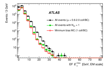
Figure 52: Distributions of $E_{\mathrm{T}}^{\mathrm{miss}}$ computed at 52 L1 and 52 the EF for all 2010 $pp$ collision events (dots) and for the subset obtained by rejecting events with multiple primary vertices (squares), compared to simulated minimum bias events that do not include pile-up effects (circles)

Figure 53: Rate of the $E_{\mathrm{T}}^{\mathrm{miss}}$ triggers at 53 L1 (L1_XE25) and 53 the EF (xe40) as a function of instantaneous luminosity for a set of runs taken near the end of 2010 running

6.6.1 Reconstruction and Selection Criteria

During 2010, the $E_{\mathrm{T}}^{\mathrm{miss}}$ and $\sum E_{\text{T}}$ triggers used calorimetric measurements calibrated at the EM scale. In the L1 calorimeter trigger system trigger towers are used to compute both $E_{\mathrm{T}}^{\mathrm{miss}}$ and $\sum E_{\text{T}}$ over the full ATLAS acceptance ($|\eta|<4.9$). The magnitude of $E_{\mathrm{T}}^{\mathrm{miss}}$ is not calculated directly at L1, but rather is derived from a look-up table that takes the values of $\Sigma$$E_{x}$ and $\Sigma$$E_{y}$ (expressed in integer values in GeV) as inputs bib:metpubnote . The resulting resolution smearing is $\sim 1~{}{\mathrm{\ Ge\kern-1.00006ptV}}$. The noise suppression scheme adopted at L1 in 2010 was very conservative with a rather high $E_{\mathrm{T}}$ threshold, in the range $1.0-1.3~{}{\mathrm{\ Ge\kern-1.00006ptV}}$, applied to each trigger tower before computing the sums $\Sigma$$E_{x}$, $\Sigma$$E_{y}$ and $E_{\mathrm{T}}^{\mathrm{miss}}$.

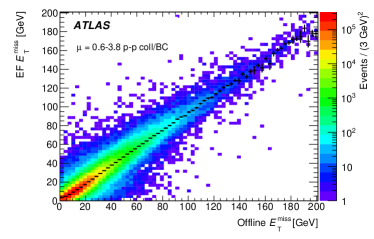
Figure 54: Correlation between the trigger and offline $E_{\mathrm{T}}^{\mathrm{miss}}$ shown for 54 L1 and 54 the EF for events triggered by the mu13 trigger. The black crosses show the mean value of online $E_{\mathrm{T}}^{\mathrm{miss}}$ calculated in each vertical slice with the vertical length of the cross representing the error on the mean. Energies are at EM scale

Figure 55: Correlation between the trigger and offline $\sum E_{\text{T}}$ measurements shown for 55 L1 and 55 the EF for events triggered by the mu13 trigger. The black crosses have the same meaning as in Fig. 54. Energies are at EM scale

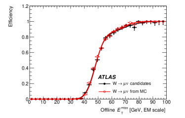
Figure 56: Efficiency of the $E_{\mathrm{T}}^{\mathrm{miss}}$ trigger as a function of offline $E_{\mathrm{T}}^{\mathrm{miss}}$ for 56 the $25{\mathrm{\ Ge\kern-1.00006ptV}}$ L1 threshold and 56 the $40{\mathrm{\ Ge\kern-1.00006ptV}}$ EF threshold, for $W\rightarrow\mu\nu$ candidates selected offline and a sample of simulated $W\rightarrow\mu\nu$ events

The discreteness of the L1 approach is smoothed out at L2, where the $\Sigma$$E_{x}$ and $\Sigma$$E_{y}$ values from L1 are summed in quadrature and a threshold is placed on the magnitude of $E_{\mathrm{T}}^{\mathrm{miss}}$=$\sqrt{({\Sigma}E_{x})^{2}+({\Sigma}E_{y})^{2}}$. At L2, the L1 energy measurement can also be corrected using the measured momenta of detected muons in the event. Since the muon correction has only a small impact on trigger rates, for 2010 running the correction was calculated at L2 and the value of the correction stored in the event. However, this correction was not applied to the $E_{\mathrm{T}}^{\mathrm{miss}}$ value calculated online, and thus was not used in the trigger decision.

Because recalculation of $E_{\mathrm{T}}^{\mathrm{miss}}$ and $\sum E_{\text{T}}$ using the full granularity of the calorimeters requires access to the whole event, it is only performed at the EF. Both $E_{\mathrm{T}}^{\mathrm{miss}}$ and $\sum E_{\text{T}}$ are estimated by the same algorithm, which loops over all calorimeter cells discarding those whose energy is negative or has a value less than three standard deviations of the noise distribution. For each of the cells with energy above threshold, an energy vector is defined whose direction is given by the unit vector starting from the nominal interaction point and pointing to the cell centre, with magnitude equal to the measured cell energy.

6.6.2 Menu and Rates

Table 11: Principal $E_{\mathrm{T}}^{\mathrm{miss}}$  and $\sum E_{\text{T}}$ triggers and their rates at a luminosity of $10^{32}\,\text{cm}^{-2}\text{s}^{-1}$

Trigger	Motivation	Rate [Hz]
xe40	$W$, top, new physics	3
te350	new physics	3

There are eight L1 $E_{\mathrm{T}}^{\mathrm{miss}}$ thresholds shown in Table 1. The L2 (EF) thresholds were set at least $2{\mathrm{\ Ge\kern-1.00006ptV}}$ ($10{\mathrm{\ Ge\kern-1.00006ptV}}$) higher than the corresponding thresholds at L1 to mask the reduced granularity of the look-up table and the effects of the slowly increasing efficiency at L1. For example the xe40 trigger has a 25 GeV threshold at L1 (L1_XE25) and a 30 GeV threshold at L2 (L2_xe30). To control the trigger rate as the instantaneous luminosity increased it was necessary to reduce the energy difference between the L1 and EF thresholds for some chains; these chains were suffixed with “tight” in the trigger menu, e.g. xe30_tight. For these triggers, the effect of the L1 efficiency turn-on extends above the EF threshold. The principal $E_{\mathrm{T}}^{\mathrm{miss}}$ and $\sum E_{\text{T}}$ triggers used in 2010 and their rates at a luminosity of $10^{32}\,\text{cm}^{-2}\text{s}^{-1}$ are shown in Table 11.

Figure 52 shows the impact of in-time pile-up on $E_{\mathrm{T}}^{\mathrm{miss}}$. The measured L1 and EF distributions are compared to a MC sample of minimum bias events simulated without pile-up. The simulation reproduces the $E_{\mathrm{T}}^{\mathrm{miss}}$ distributions for the bunch crossings with a single $pp$ collision ($N_{pv}~{}=~{}1$). For data events with multiple collisions (0.6-2.0 collisions/BC) there is a visible broadening of the $E_{\mathrm{T}}^{\mathrm{miss}}$ distribution reflecting an increase in $E_{\mathrm{T}}^{\mathrm{miss}}$ due to pile-up. The $E_{\mathrm{T}}^{\mathrm{miss}}$ trigger rates at L1 and the EF are shown in Fig. 53 for the xe40 trigger which has a 25 GeV threshold at L1 (L1_XE25) and a 40 GeV thresholds at the EF. The $E_{\mathrm{T}}^{\mathrm{miss}}$ rate rate increase with luminosity is faster than linear, due to the effects of pile-up.

6.6.3 Resolution

The correlations between the trigger and offline values of $E_{\mathrm{T}}^{\mathrm{miss}}$ and $\sum E_{\text{T}}$ using uncalibrated calorimeter energies are shown in Figs. 54 and 55. The offline calculations use an algorithm (MET_Topo) which sums the energy deposited in topological clusters ATL-LARG-PUB-2008-002 . Figure 54 shows the correlation between L1 and offline $E_{\mathrm{T}}^{\mathrm{miss}}$ for events triggered by the mu13 trigger (Section 6.3). The L1 $E_{\mathrm{T}}^{\mathrm{miss}}$ resolution is worse than offline, as expected, while the EF shows a good correlation and improved resolution with respect to L1, as seen in Fig. 54. Figure 55 shows the correlation between the L1 $\sum E_{\text{T}}$ and that calculated by the offline algorithm MET_Topo for events selected by the mu13 trigger. L1 underestimates the $\sum E_{\text{T}}$  particularly at low values, due to the rather conservative noise suppression (i.e. high trigger tower $E_{\mathrm{T}}$ thresholds) employed at L1. The effect is to shift the energy scale at low $\sum E_{\text{T}}$ values, as shown by the non-linear behaviour in Figure 55.

The plot in Fig. 55 shows the correlation between the EF and offline values of $\sum E_{\text{T}}$. There is an offset of about $10{\mathrm{\ Ge\kern-1.00006ptV}}$ for the values of $\sum E_{\text{T}}$ computed at EF, as the offline $\sum E_{\text{T}}$ approaches zero. The offset arises because of a one-sided noise cut applied by the trigger, compared to symmetric cuts applied offline. The main motivation for the choice made at the EF is to protect against large negative energy values, which could arise from read-out problems and which would constitute a source of fake $E_{\mathrm{T}}^{\mathrm{miss}}$. The choice of the online noise cut (of three times the r.m.s. noise) is a compromise between minimising the offset (a lower cut of twice the r.m.s. noise would give a much larger bias of $\sim 200{\mathrm{\ Ge\kern-1.00006ptV}}$) and maintaining sensitivity, since higher thresholds would cause a greater loss of the real signal bib:metpubnote .

6.6.4 Efficiency

Figure 57: Efficiency of 57 the L1 $\sum E_{\text{T}}$ threshold at 50 GeV and 57 the EF-only $\sum E_{\text{T}}$ threshold at $200{\mathrm{\ Ge\kern-1.00006ptV}}$, as a function of $\sum E_{\text{T}}$ calculated by the offline algorithm MET_Topo, for $W\rightarrow\mu\nu$ candidates selected offline and a sample of simulated $W\rightarrow\mu\nu$ events

Figure 56 shows the efficiency of the L1 $E_{\mathrm{T}}^{\mathrm{miss}}$ trigger with a $25{\mathrm{\ Ge\kern-1.00006ptV}}$ threshold as a function of $E_{\mathrm{T}}^{\mathrm{miss}}$ reconstructed offline for $W\rightarrow\mu\nu$ candidates selected in offline reconstruction, triggered by mu13. The plateau region is described well by the MC. The agreement with the simulation is not perfect for low energies; background events from QCD processes and $W$ boson decays into taus, which subsequently decay into muons, are difficult to simulate precisely. Figure 56 shows the corresponding efficiency for the full trigger chain including a $40{\mathrm{\ Ge\kern-1.00006ptV}}$ $E_{\mathrm{T}}^{\mathrm{miss}}$ threshold at EF. The initial faster rise of the efficiency turn-on is dominated by the EF $E_{\mathrm{T}}^{\mathrm{miss}}$ resolution whereas the slower rise approaching the plateau is due to the slower L1 turn-on. This behaviour is modelled well by the simulation. Once the plateau has been reached the $E_{\mathrm{T}}^{\mathrm{miss}}$ triggers remain fully efficient within a negligible systematic uncertainty.

Figure 57 shows the L1 efficiency turn-on for a nominal $\sum E_{\text{T}}$ threshold of $50{\mathrm{\ Ge\kern-1.00006ptV}}$. The late turn-on, starting only at about 150 GeV in offline $\sum E_{\text{T}}$, results from an under-estimation of $\sum E_{\text{T}}$ at L1 due to the noise suppression scheme, as described in subsection 6.6.3. The efficiency reaches 90% at about $260{\mathrm{\ Ge\kern-1.00006ptV}}$. Data and MC agree reasonably well; the shift in the efficiency turn-on is due to small errors in the modelling of noise at the individual cell level in the simulation. Figure 57 shows the efficiency of the EF selection alone, not including L1 and L2. The EF efficiency reaches 90% at about $230{\mathrm{\ Ge\kern-1.00006ptV}}$. Once the plateau has been reached the $\sum E_{\text{T}}$ triggers remain fully efficient within a negligible systematic uncertainty. Data and simulation agree well. More details can be found in Ref. bib:metconfnote .

6.7 $b$-Jets

The ability to separate heavy flavour jets from light-quark and gluon jets is an important asset for many physics analyses, such as measurements in the top-quark sector and searches for Higgs bosons or other new physics signatures. The ability to identify $b$-jets in the ATLAS trigger system gives access to signals that would otherwise be lost in the multi-jet background, such as $t\bar{t}\to jets$. ATLAS employs two categories of $b$-jet triggers: lifetime triggers that exploit the $B$-hadron time-of-flight and muon-jet triggers that exploit the presence of a muon in $B$-hadron decays.

During the 2010 data-taking period, the lifetime triggers were not in active rejection mode and the muon-jet triggers were used to collect data to validate the lifetime triggers. The lifetime triggers will be used in 2011 to collect data for physics analysis. In this section a brief description of the muon-jet triggers is given, but the main focus is on the performance of the lifetime triggers.

6.7.1 $b$-Jets Reconstruction and Selection Criteria

Muon-jet triggers were used to select events containing jets associated with a low $p_{\mathrm{T}}$ muon. At L1 a combined muon-jet trigger, L1_MU0_JX (X=5,10,15,30,55), required the lowest threshold muon trigger in combination with a jet. No topological matching between muon and jet is possible at L1. The HLT selection introduces a refinement of the muon selection (L2_mu4) and requires matching within $\Delta R<0.4$ between the muon and the corresponding L1 jet. The selected jet sample is enriched in $b$-jets and is used to calibrate both trigger and offline $b$-tagging algorithms.

Lifetime triggers use tracks and vertices reconstructed at the HLT (in the region $\eta<2.5$) to select a sample enriched in $b$-jets. These triggers are based on the impact parameters of tracks with respect to the reconstructed primary vertex. The HLT selection is based on inner detector tracks reconstructed within a L1 jet RoI. The lowest threshold $b$-jet trigger is b10 which starts from a L1 jet with a $10{\mathrm{\ Ge\kern-1.00006ptV}}$ $E_{\mathrm{T}}$ threshold (L1_J10).

At the HLT, the first step for the lifetime triggers is to find the location of the primary vertex. The coordinates of the primary vertex in the transverse plane are determined by the beamspot information which is part of the configuration data provided to the algorithm via the online conditions database. The beamspot position can be updated during a run based on information from the online beamspot measurement (Section 5.2). During 2010 running, when the lifetime triggers were not in active rejection mode, this update was initiated manually whenever the beamspot showed a significant displacement. The longitudinal coordinate of the primary vertex is determined on an event-by-event basis from a histogram of the $z$ positions of all tracks in the RoI. The $z$ position of the vertex is identified, using a sliding window algorithm, as the $z$ position at which the window contains the most histogram entries. In the case of multiple primary vertices, this algorithm selects the vertex with the most tracks.

The transverse and longitudinal impact parameters are determined, for each track, as the distances from the primary vertex to the point of closest approach of the track, in the appropriate projection. The impact parameters are signed with respect to the jet axis determined by a track-based cone jet reconstruction algorithm. The impact parameter is positive if the angle between the jet axis and a line from the primary vertex to the point of closest approach of the track is less than $90^{\circ}$.

Two different methods, likelihood and $\chi^{2}$ taggers, both based on the track impact parameters, are then used to build a variable discriminating between $b$ and light jets:

•

Likelihood taggers: longitudinal and transverse impact parameters are combined, using a likelihood ratio method, to form a discriminant variable.

•

$\chi^{2}$ tagger: the compatibility of the tracks in the RoI with the beamspot is tested using the transverse impact parameter significance (defined as the transverse impact parameter divided by the transverse impact parameter resolution) aleph:JetProb . The distribution of the $\chi^{2}$ probability of the impact parameter significance for all the tracks reconstructed in an RoI is expected to be uniform for light jets, as tracks come from the primary vertex, while it peaks toward 0 for $b$-jets, which contain tracks that are not from the primary vertex. The $\chi^{2}$ probability can, therefore, be used as a discriminant variable. It is set to 1 for RoIs that do not contain any reconstructed tracks.

Likelihood taggers are more powerful, in principle, but require significant validation from data as they rely on determining probability density functions that give the signal and background probabilities corresponding to a given impact parameter value. The $\chi^{2}$ tagger, though less powerful, can be tuned more easily on data using the negative side of the transverse impact parameter distribution. This technique is used because the shape of the negative side of the distribution is determined only by resolution effects and there is no significant contribution from highly displaced tracks in this part of the distribution.

Figure 58: The $\chi^{2}$ probability distribution before and after the beamspot measurement update in a data-taking period when the beamspot was significantly displaced with respect to the reference

The importance of the online beamspot measurement is demonstrated in Fig. 58 which shows the $\chi^{2}$ probability distribution of the $\chi^{2}$ tagger before and after a beamspot update in a data-taking period when the beamspot was significantly displaced with respect to the initial reference. In 2011 the beamspot will be updated automatically every few minutes because a transverse displacement of the beamspot can cause tracks in light-quark jets to artificially acquire large impact parameters and so resemble the tracks in $b$-jets.

6.7.2 $b$-Jets Menu and Rates

During the 2010 data-taking period the muon-jet triggers were the only $b$-jet triggers in active rejection mode, selecting the calibration sample. The lifetime triggers ran in monitoring mode, allowing for tuning in preparation for activation in 2011 running. Similar algorithms ran at both L2 and the EF.

The muon-jet triggers were maintained at a rate of about 7 Hz, using prescaling when luminosity exceeded $10^{31}\,\text{cm}^{-2}\text{s}^{-1}$. Prescaling of the triggers with lower jet thresholds was done in such a way as to collect a sample of events with a uniform jet transverse momentum distribution in the reconstructed muon-jet pairs. The uniformity of the distribution is important for a precise determination of the $b$-jet efficiency in a wide range of jet transverse momenta.

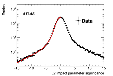
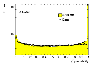
Figure 59: 59 Transverse impact parameter significance distribution for L2 tracks with a fit to the negative side. 59 $\chi^{2}$ distribution in data and simulation after tuning procedure

6.7.3 $b$-Jet Trigger Performance

The performance of the $\chi^{2}$ tagger is shown in Table 12, which gives the rejection obtained from data collected with the b10 trigger and the efficiency obtained from simulation of $b$-jets with a similar $p_{\mathrm{T}}$ distribution to the data. The efficiency measurement from simulation requires a tagged jet RoI matched with an offline jet ($\Delta R<0.4$). The offline jet is required to be associated with a true $b$ quark ($\Delta R<0.3$) and identified by an offline tagger based on the secondary vertex transverse flight length significance.

Table 12: Single $b$-RoI efficiency and rejection for the $\chi^{2}$ tagger at L2 and for the HLT. The efficiency is computed using MC with respect to tagged offline $b$-jets while rejection is computed on data

Efficiency	L2 Rejection	HLT Rejection
0.7	2	8
0.6	3	17
0.5	6	28

The data collected with the b10 trigger has been used to tune the $\chi^{2}$ tagger ready for the activation of the $b$-jet trigger in 2011 data-taking. The tuning procedure is identical for L2 and EF and consists mainly of a parameterization of the transverse impact parameter resolution. The selection cuts applied at L2 and the EF are chosen to give the optimum overall balance of efficiency and rejection at each level, taking into account the different impact parameter resolutions of the L2 and EF tracking algorithms (Section 5.1). Figure 59 shows the L2 transverse impact parameter significance distribution for data, where the impact parameter is signed with respect to the jet axis. The negative side of this distribution is mainly due to tracks originating from light quarks decays, allowing the resolution to be studied using an almost pure sample of tracks coming from the primary vertex. A fit was made to the negative part of the impact parameter significance distribution using a double Gaussian function. The result of the fit is shown superimposed on the data points in Fig. 59. The same tuning procedure was applied separately to MC simulated data. The $\chi^{2}$ probability distributions obtained using the parameterized resolution are shown in Fig. 59 for data and simulation. Data and MC simulation show reasonable agreement, although there are some differences at values of the $\chi^{2}$ probability close to 0 and 1. A typical cut would be to select jets with a $\chi^{2}$ probability less than 0.07. The peak at 1 reflects the choice of setting the $\chi^{2}$ probability to 1 for RoIs that do not contain any reconstructed tracks.

6.8 $B$-Physics

The ATLAS $B$-physics programme includes searches for rare $B$ hadron decays and CP violation measurements, as well as tests of QCD calculations through production and spin-alignment measurements of heavy flavour quarkonia and $B$ baryons bib:BphysUpsilon ; bib:BphysJpsi . $B$-physics triggers complement the low-$p_{\mathrm{T}}$ muon triggers by providing invariant mass based selections for $J/\psi$, $\mit\Upsilon$, and $B$ mesons. There are two categories of $B$-physics triggers, topological and single RoI seeded, each one exploiting a different characteristic of the ATLAS trigger system to manage the event rates.

6.8.1 $B$-Physics Reconstruction and Selection Criteria

Table 13: $B$-physics primary trigger menu and rates at a luminosity of $10^{32}\,\text{cm}^{-2}\text{s}^{-1}$

Trigger	Motivation	Rate [Hz]
mu4_DiMu	a loose single RoI seeded trigger	8
mu4_DiMu_FS	a loose single RoI seeded trigger using FullScan	13
mu4_Jpsimumu	a single RoI seeded selection for $J/\psi$	3
mu4_Upsimumu_FS	a single RoI seeded selection for $\mit\Upsilon$	3
mu4_Bmumu	a single RoI seeded selection for $B$ mesons	$<$1
2mu4_DiMu	a loose topological selection	4
2mu4_Jpsimumu	topological selection for $J/\psi$	1
2mu4_Upsimumu	topological selection for $\mit\Upsilon$	$<$1
2mu4_Bmumu	topological selection for $B$ mesons	$<$1

•

Topological triggers require 2 muon RoIs to have been found at L1 and the HLT (see Section 6.3). The $B$-physics algorithms in the HLT then combine the information from the two muon RoIs to search for the parent $J/\psi$, $\mit\Upsilon$, or $B$ meson, and a vertex fit is performed for the two reconstructed ID tracks. The requirement for two muons at L1 reduces the rate, but is inefficient for events where the second muon does not give rise to a L1 RoI because it has low momentum, or falls outside the L1 acceptance.

•

Single RoI seeded triggers recover events that have been missed by the topological triggers by starting from a single L1 muon and finding the second muon at the HLT. In this approach, tracking is performed in a large region ($\Delta\eta\times\Delta\phi=1.5\times 1.5$) around the L1 muon. At L2, tracks found in this large RoI are extrapolated to the muon system. The algorithm searches for muon hits within a road around the extrapolated track; if enough hits are found then the track is flagged as a muon. At the EF the search for tracks within the large RoI uses the EF Combined strategy (Section 5.4) which starts from the Muon Spectrometer and then adds inner detector information. If a second track is found, it is combined with the first one to search for the parent di-muon object in the same way as in the topological trigger. This approach can also be used in FullScan (FS) mode (Section 5.1). The FS mode is particularly useful for triggering $\mit\Upsilon$ events where the muons tend to be separated by more than the RoI size, but requires approximately 8 times more CPU time than the RoI approach.

In both approaches, a series of cuts can be made on the muon pair requiring: the two muons are opposite charge; the mass cuts $J/\psi$: $2.5-4.3{\mathrm{\ Ge\kern-1.00006ptV}}$, $\mit\Upsilon$: $8-12{\mathrm{\ Ge\kern-1.00006ptV}}$, $B$: $4-7{\mathrm{\ Ge\kern-1.00006ptV}}$, DiMu $>0.5{\mathrm{\ Ge\kern-1.00006ptV}}$; a cut on the $\chi^{2}$ of the reconstructed vertex. The mass cuts are very loose compared to the mass resolutions ($\sim$40 MeV and $\sim$100 MeV for $J/\psi$ and $\mit\Upsilon$ respectively). In 2010 chains were run both with and without the opposite sign requirement and with and without a requirement on the vertex $\chi^{2}$.

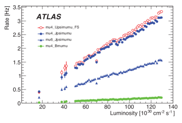
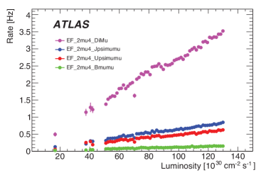
Figure 60: Plot of rates for several triggers for 60 single RoI seeded chains and 60 topological chains.

6.8.2 $B$-Physics Trigger Menu and Rates

Table 13 gives an overview of the main $B$-physics triggers and their rates at a luminosity of $10^{32}\,\text{cm}^{-2}\text{s}^{-1}$. At this luminosity the mu4 trigger was prescaled by 1500 and the 2mu4 trigger was prescaled by 85. The single muon-seeded “DiMu” triggers needed to be prescaled by $\sim$20; however the topological triggers ran unprescaled. Figure 60 shows the rates for some of the triggers shown in Table 13 as a function of instantaneous luminosity.

6.8.3 $B$-Physics Trigger Efficiency

The efficiencies of the $B$-physics triggers have been measured from data using triggers in monitoring mode (Section 3). The efficiencies of the mu4_Jpsimumu trigger with respect to L1_MU0 and the 2mu4_Jpsimumu trigger with respect to L1_2MU0 are shown in Fig. 61 for events containing a $J/\psi\rightarrow\mathrm{\mu\mu}$ decay reconstructed offline with both muon’s $p_{\mathrm{T}}>4{\mathrm{\ Ge\kern-1.00006ptV}}$. The efficiencies shown in Fig. 61 include the HLT muon trigger efficiencies and the efficiency of the subsequent $J/\psi\rightarrow\mathrm{\mu\mu}$ selection cuts. The efficiencies have been determined within a systematic uncertainty of less than 1%; statistical uncertainties are presented in the figures.

In order to show the efficiency of the $J/\psi\rightarrow\mathrm{\mu\mu}$ selection itself, independent of the muon trigger, Fig. 61 shows the efficiency of: the single RoI-seeded mu4_Jpsimumu trigger with respect to the mu4 trigger; the topological 2mu4_Jpsimumu trigger with respect to the 2mu4 trigger; and the topological 2mu4_Jpsimumu trigger with respect to the mu4 trigger. The mu4_Jpsimumu trigger has an efficiency of 85% with respect to mu4 including the efficiency to reconstruct the second muon at the HLT, which causes a reduction of efficiency for low $p_{\mathrm{T}}$ $J/\psi$. The benefit of using single RoI triggers is shown by comparing the mu4_Jpsimumu trigger efficiency with the lower efficiency of 50% for the 2mu4_Jpsimumu trigger with respect to the mu4 trigger. The lower efficiency of the topological trigger results mainly from the requirement for a second L1 muon; the efficiency of the 2mu4_Jpsimumu trigger is 92% for events with a 2mu4 trigger.

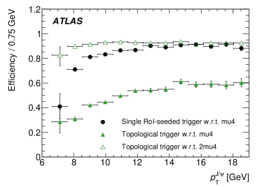
Figure 61: Efficiencies for $J/\psi\rightarrow\mathrm{\mu\mu}$ events selected offline as a function of the $J/\psi$  $p_{\mathrm{T}}$  for 61 the single RoI-seeded mu4_Jpsimumu trigger with respect to L1_MU0 and the topological 2mu4_Jpsimumu trigger with respect to L1_2MU0 and 61 the mu4_Jpsimumu trigger with respect to the mu4 trigger and the 2mu4_Jpsimumu with respect to the mu4 and 2mu4 triggers

7 Overall Trigger Performance

In this section the overall performance of the ATLAS trigger is presented. Overall trigger performance parameters include the total rates at each trigger level, the CPU processing time per event, and the load on CPU resources available at L2 and EF. To demonstrate these performance parameters, a run from period I was selected which took place during the last $pp$ fill of 2010 and had instantaneous luminosities ranging from $0.85\times 10^{32}\,\text{cm}^{-2}\text{s}^{-1}$ to $1.8\times 10^{32}\,\text{cm}^{-2}\text{s}^{-1}$. This run was 15 hours long and had an integrated luminosity of 6.4 pb^-1.

7.1 Total Trigger Rates

The total L1, L2, and EF output rates are given in Fig. 62 as a function of instantaneous luminosity for the sample run from period I. By changing prescale factors as the luminosity fell, the trigger rates were kept stable throughout the run at $\sim$30 kHz (L1), $\sim$4 kHz (L2), and $\sim$450 Hz (EF). The prescale factor changes can be seen in the figures as discontinuities in the rate as a function of luminosity. Prescale factors at L2 and EF are changed at the same time, while L1 prescale factors are set independently. The output rates for each stream in the same run are given in Fig. 62. The relative fractions of each stream are tuned as a function of instantaneous luminosity in order to optimize the total rate and physics yield.

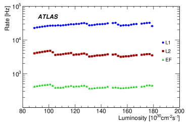
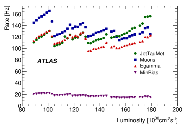
Figure 62: Total output trigger rates as a function of instantaneous luminosity in a sample run from period I for 62 each trigger level and 62 each stream. B-jet triggers are included in the JetTauEtmiss stream and B-physics triggers are included in the muon stream

ATLAS utilizes an inclusive streaming scheme, meaning that an event that fires a trigger in two different streams will be written twice, once in each stream, creating some overlap between different streams. The only pairs of streams that show a significant overlap ($>$1%) at $\mathcal{L}$=$10^{32}\,\text{cm}^{-2}\text{s}^{-1}$ are: Egamma-JetTauEtmiss 14%, Egamma-Muons 2%, and Muons-JetTauEtmiss 4%. At higher instantaneous luminosity, when the lower $p_{\mathrm{T}}$ threshold items will have higher prescales, the Egamma-JetTauEtmiss overlap will decrease. The goal is to keep the total overlap between streams below 10%.

7.2 Timing

The timing performance of the individual algorithms has been discussed throughout the paper. Figure 63 shows the total processing time per event in the sample run for L2 and EF.

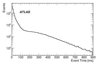
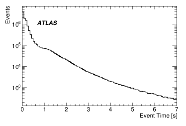
Figure 63: Processing time per event for 63 L2 and 63 EF in the sample run

Figure 64 presents the mean processing time per event at L2 and EF as a function of instantaneous luminosity; L2 is further subdivided into the mean time to retrieve data over the network from the Read out Buffers (ROB time) and the computational time taken by the algorithms (CPU time). The figure shows that L2 was running close to the design limit of $\sim 40$ms and EF was running at $\sim 400$ms, well below the design limit of $\sim 4$s. Figure 64, reporting the fraction of CPU used in the HLT farm, shows that the HLT farm was well within its CPU capacity. As was the the case for the trigger rates, discontinuities in the CPU usage with luminosity are due to deliberate changes of prescale sets to control the trigger rate.

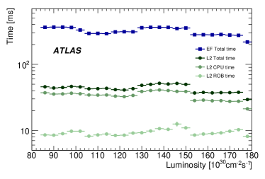
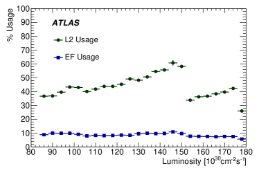
Figure 64: 64 Mean time per event and 64 fraction of trigger system CPU usage for L2 and EF as function of luminosity in the sample run

Table 14: The bandwidth allocation guidelines per trigger group for 2011 for a total rate of $\sim$200Hz. For primary physics triggers, the L1 and HLT thresholds and predicted trigger rates are given for a luminosity of $10^{33}\,\text{cm}^{-2}\text{s}^{-1}$

	$p_{T}$ threshold [GeV]
Category	L1	HLT	Rate [Hz]	Bandwidth [Hz]
minbias, zerobias				10
muon				45
single muon	10	20	25
di-muon	4	10	3
$B$-physics				15
Jpsimumu			8
Upsimumu			4
Rare B decays			3
$e/\gamma$				55
single electron	14	20	20
di-electron	7	12	0.5
electron + muon	5(e),4($\mu$)	10(e),6($\mu$)	3.5
single photon	14	80	1
di-photon	14	20	1.5
tau, tau+$E_{\mathrm{T}}^{\mathrm{miss}}$				30
single tau	30	100	4
di-tau	11	29	4
tau+electron	6($\tau$),10(e)	16($\tau$),15($\mu$)	3
tau+muon	6($\tau$),4($\mu$)	16($\tau$),15($\mu$)	5
jet, $b$-jet, jet+$E_{\mathrm{T}}^{\mathrm{miss}}$				55
jet+$E_{\mathrm{T}}^{\mathrm{miss}}$	50(jet),20($E_{\mathrm{T}}^{\mathrm{miss}}$)	75(jet),45($E_{\mathrm{T}}^{\mathrm{miss}}$)	15
single jet	75	250	3
single forward jet	50	100	3
multi-jets (with $b$-tagging)	10		8
$E_{\mathrm{T}}^{\mathrm{miss}}$, $\sum E_{\text{T}}$, exotics				10
calibration & commissioning				10

8 Outlook

The trigger menus for 2011 and 2012 running will cover instantaneous luminosities from $\sim 10^{32}\,\text{cm}^{-2}\text{s}^{-1}$ to $\sim 5\cdot 10^{33}\,\text{cm}^{-2}\text{s}^{-1}$ at $\sqrt{s}={7}{\mathrm{\ Te\kern-1.00006ptV}}$ with around 10-23 $pp$ interactions per bunch crossing and a 50 ns bunch spacing. At these instantaneous luminosities the main triggers will select electrons and muons with $p_{\mathrm{T}}$ above about $20{\mathrm{\ Ge\kern-1.00006ptV}}$, jets with $p_{\mathrm{T}}$ above about $200{\mathrm{\ Ge\kern-1.00006ptV}}$, $E_{\mathrm{T}}^{\mathrm{miss}}$ above about $50{\mathrm{\ Ge\kern-1.00006ptV}}$, as well as $E_{\mathrm{T}}^{\mathrm{miss}}$ in combination with a tau or jet. The primary triggers are shown in Table 14 together with the L1 and HLT thresholds and predicted trigger rates for a luminosity of $10^{33}\,\text{cm}^{-2}\text{s}^{-1}$.

The table also shows the bandwidth allocation guidelines for each group of triggers. The primary triggers make up about two thirds of the output bandwidth. The remainder of the bandwidth is filled with supporting, commissioning, calibration, and monitoring triggers. Supporting triggers populate the largest part of the remaining bandwidth. For example, prescaled jet and photon supporting triggers provide an approximately flat event yield as a function of $p_{\mathrm{T}}$ to be used for measurements limited by systematic uncertainties. In addition, a smaller fraction of bandwidth is allocated to commissioning triggers specifically intended for the further development of the trigger menu. The total number of triggers is reduced compared to 2010 menus, as many items necessary for commissioning or lower luminosities are removed.

In contrast to the rapid evolution in 2010, the 2011/12 LHC conditions will be increasingly stable, and changes in the trigger menu will be less frequent than in 2010. Daily changes will be limited to adjustments of prescales, mainly for monitoring and commissioning triggers. To improve the stability of the data recorded for physics analysis, changes to primary triggers and re-tuning of the menu is limited to monthly updates. The trigger will, however, continue to evolve to match LHC luminosity and beam conditions.

9 Conclusion

The ATLAS trigger system has been commissioned and has successfully delivered data for ATLAS physics analysis. Efficiencies, which meet the original design criteria, have been determined from data. These include overall trigger efficiencies of: greater than $99\%$ for electrons and photons with $E_{\mathrm{T}}>25~{}GeV$; $94-96$% for muons with $p_{\mathrm{T}}>13~{}GeV$, in the regions of full acceptance; greater than $90$% for tau leptons with $p_{\mathrm{T}}>30~{}GeV$; greater than $99$% for jets with $E_{\mathrm{T}}>60~{}GeV$. The missing $E_{\mathrm{T}}$ trigger was fully efficient above $100~{}{\mathrm{\ Ge\kern-1.00006ptV}}$ throughout the 2010 data-taking period. Quantities calculated online, using fast trigger algorithms, show excellent agreement with those reconstructed offline. Data and simulation agree well for these quantities and for measured trigger efficiencies.

The trigger system has been demonstrated to function well, satisfying operational requirements and evolving to meet the demands of rapidly increasing LHC luminosity. Trigger menus will continue to evolve to fulfil future demands via progressive increase of prescales, tightening of selection cuts, application of isolation requirements, and increased use of multi-object and combined triggers. The excellent performance of the trigger system in 2010 and the results of studies confirming the scaling to higher luminosities give confidence that the ATLAS trigger system will continue to meet the challenges of running in 2011 and beyond.

References

- (1) The ATLAS Collaboration, The ATLAS Experiment at the CERN Large Hadron Collider., JINST 3 (2008) S08003.
- (2) L. Evans and P. Bryant, LHC Machine., JINST 3 (2008) S08001.
- (3) T. Sjostrand, S. Mrenna, and P. Z. Skands, PYTHIA 6.4 Physics and Manual, JHEP 0605 (2006) 026.
- (4) The ATLAS Collaboration, ATLAS Monte Carlo tunes for MC09, Tech. Rep. ATL-PHYS-PUB-2010-002, CERN, Geneva, 2010. http://cdsweb.cern.ch/record/1247375.
- (5) S. Agostinelli et al., GEANT4: a simulation toolkit, Nucl. Instrum. Meth. 506 (2003) no. 3, 250 – 303.
- (6) The ATLAS Collaboration, The ATLAS simulation infrastructure, Eur. Phys. J. C 70 (2010) 823–874.
- (7) The ATLAS Collaboration, Commissioning of the ATLAS Muon Spectrometer with cosmic rays., Eur. Phys. J. C 70 (2010) 875–916.
- (8) S. Ask et al., The ATLAS central level-1 trigger logic and TTC system, JINST 3 (2008) P08002.
- (9) R. Achenbach et al., The ATLAS level-1 calorimeter trigger, JINST 3:P03001 (2008) 1–39.
- (10) The ATLAS Collaboration, Expected performance of the ATLAS experiment : detector, trigger and physics, arXiv:0901.0512.
- (11) R. Fruhwirth, Application of Kalman filtering to track and vertex fitting, Nucl. Instrum. Meth. A262 (1987) 444.
- (12) T. Cornelissen et al., Concepts, design and implementation of the ATLAS New Tracking (NEWT), Tech. Rep. ATL-SOFT-PUB-2007-007, CERN, Geneva, 2007. http://cdsweb.cern.ch/record/1020106?ln=en.
- (13) The ATLAS Collaboration, Characterization of interaction-point beam parameters using the pp event-vertex distribution reconstructed in the ATLAS detector at the LHC, ATLAS-CONF-2010-027 (2010) . http://cdsweb.cern.ch/record/1277659.
- (14) W. Lampl et al., Calorimeter clustering algorithms: description and performance, Tech. Rep. ATL-LARG-PUB-2008-002, CERN, Geneva, 2008. http://cdsweb.cern.ch/record/1099735.
- (15) M.Cacciari et al., The anti-kt jet clustering algorithm, JHEP 0804 (2008) 063.
- (16) The ATLAS Collaboration, Measurement of underlying event characteristics using charged particles in pp collisions at = 900 GeV and 7 TeV with the ATLAS detector, Eur. Phys. J. C 71 (2011) 1–24.
- (17) The ATLAS Collaboration, Charged-particle multiplicities in pp interactions measured with the ATLAS detector at the LHC, New Journal of Physics 13 (2011) no. 5, 053033.
- (18) The ATLAS Collaboration, Observation of a centrality-dependent dijet asymmetry in lead-lead collisions at = 2.76 TeV with the ATLAS detector at the LHC, Phys. Rev. Lett. 105 (2010) 252303.
- (19) The ATLAS Collaboration, Performance of the minimum bias trigger in p-p collisions at = 7 TeV, ATLAS-CONF-2010-068 (2010) . http://cdsweb.cern.ch/record/1281343.
- (20) The ATLAS Collaboration, Measurement of the and production cross sections in proton-proton collisions at = 7 TeV with the ATLAS detector, JHEP 12 (2010) 060.
- (21) The ATLAS Collaboration, Measurement of the top quark-pair production cross section with ATLAS in pp collisions at =7 TeV, Eur. Phys. J. C 71 (2011) 1577.
- (22) The ATLAS Collaboration, Measurement of the inclusive isolated prompt photon cross-section in pp collisions at = 7 TeV with the ATLAS detector., Phys. Rev. D 83 (2011) 052005.
- (23) The ATLAS Collaboration, Measurement of the production cross section for W-bosons in association with jets in pp collisions at =7 with the ATLAS detector, Phys. Lett. B 698 (2010) 325–345.
- (24) The ATLAS Collaboration, Search for diphoton events with large missing transverse energy in 7 TeV proton-proton collisions with the ATLAS detector, Phys. Rev. Lett. 106 (2011) 121803.
- (25) The ATLAS Collaboration, Search for supersymmetry using final states with one lepton, jets, and missing transverse momentum with the ATLAS detector in =7 TeV pp collisions, Phys. Rev. Lett. 106 (2011) 131802.
- (26) The ATLAS Collaboration, Performance of the ATLAS electron and photon triggers with = 7 TeV collisions, ATLAS-CONF-2011-114 (2011) . http://cdsweb.cern.ch/record/1375551.
- (27) The ATLAS Collaboration, Measurement of the and production cross-sections in proton-proton collisions at TeV with the ATLAS detector, JHEP 2010 (2010) 1–65.
- (28) The ATLAS Collaboration, Readiness of the ATLAS Liquid Argon calorimeter for LHC collisions, Eur. Phys. J. C 70 (2010) no. 3, 723–753.
- (29) The ATLAS Collaboration, Performance of the ATLAS muon trigger in p-p collisions at = 7 TeV, ATLAS-CONF-2010-95 (2010) . http://cdsweb.cern.ch/record/1299573.
- (30) The ATLAS Collaboration, Measurement of inclusive jet and dijet cross sections in proton-proton collisions at 7 TeV centre-of-mass energy with the ATLAS detector, Eur. Phys. J. C 71 (2011) 1–59.
- (31) The ATLAS Collaboration, Study of Jet Shapes in Inclusive Jet Production in pp Collisions at = 7 TeV using the ATLAS Detector, Phys. Rev. D 83 (2011) 052003.
- (32) The ATLAS Collaboration, Search for new particles in two-jet final states in 7 TeV proton-proton collisions with the ATLAS detector at the LHC, Phys. Rev. Lett. 105 (2010) 161801.
- (33) The ATLAS Collaboration, Search for quark contact interactions in dijet angular distributions in 7 TeV proton-proton collisions with the ATLAS detector at the LHC, Phys. Lett. B 694 (2011) 327–345.
- (34) The ATLAS Collaboration, Performance of the ATLAS jet trigger from the early = 7 TeV data, ATLAS-CONF-2010-094 (2010) . http://cdsweb.cern.ch/record/1299109.
- (35) The ATLAS Collaboration, Jet energy scale and its systematic uncertainty in proton-proton collisions at sqrt(s)=7 TeV in ATLAS 2010 data, ATLAS-CONF-2011-032 (2011) . http://cdsweb.cern.ch/record/1337782.
- (36) The ATLAS Collaboration, Data-Quality requirements and event cleaning for jets and missing transverse energy reconstruction with the ATLAS detector in proton-proton collisions at a center of mass energy TeV, ATLAS-CONF-2010-038 (2010) . http://cdsweb.cern.ch/record/1277678.
- (37) The ATLAS Collaboration, Properties of jets and inputs to jet reconstruction and calibration with the ATLAS detector using proton-proton collisions at TeV, ATLAS-CONF-2010-053 (2010) . http://cdsweb.cern.ch/record/1281310.
- (38) The ATLAS Collaboration, Search for stable hadronising squarks and gluinos with the ATLAS experiment at the LHC, Phys. Lett. B 701 (2011) no. 1, 1–19.
- (39) D. Casadei et al., The implementation of the ATLAS missing Et triggers for the initial LHC operation, Tech. Rep. ATL-DAQ-PUB-2011-001, CERN, Geneva, 2011. http://cdsweb.cern.ch/record/1331180.
- (40) The ATLAS Collaboration, Performance of the ATLAS transverse energy triggers with initial LHC runs at TeV, ATLAS-CONF-2011-072 (2011) . http://cdsweb.cern.ch/record/1351836.
- (41) The ALEPH Collaboration, A precise measurement of , Phys. Lett. B 313 (1993) 535–548.
- (42) The ATLAS Collaboration, Measurement of the (1S) Production Cross-Section in pp Collisions at TeV in ATLAS, arXiv:1106.5325v1.
- (43) The ATLAS Collaboration, Measurement of the differential cross-sections of inclusive, prompt and non-prompt J/psi production in proton-proton collisions at TeV, Nucl. Phys. B 850 (2011) 387–444.
The ATLAS Collaboration
G. Aad48,
B. Abbott111,
J. Abdallah11,
A.A. Abdelalim49,
A. Abdesselam118,
O. Abdinov10,
B. Abi112,
M. Abolins88,
H. Abramowicz153,
H. Abreu115,
E. Acerbi89a,89b,
B.S. Acharya164a,164b,
D.L. Adams24,
T.N. Addy56,
J. Adelman175,
M. Aderholz99,
S. Adomeit98,
P. Adragna75,
T. Adye129,
S. Aefsky22,
J.A. Aguilar-Saavedra124b,a,
M. Aharrouche81,
S.P. Ahlen21,
F. Ahles48,
A. Ahmad148,
M. Ahsan40,
G. Aielli133a,133b,
T. Akdogan18a,
T.P.A. Åkesson79,
G. Akimoto155,
A.V. Akimov 94,
A. Akiyama67,
M.S. Alam1,
M.A. Alam76,
S. Albrand55,
M. Aleksa29,
I.N. Aleksandrov65,
F. Alessandria89a,
C. Alexa25a,
G. Alexander153,
G. Alexandre49,
T. Alexopoulos9,
M. Alhroob20,
M. Aliev15,
G. Alimonti89a,
J. Alison120,
M. Aliyev10,
P.P. Allport73,
S.E. Allwood-Spiers53,
J. Almond82,
A. Aloisio102a,102b,
R. Alon171,
A. Alonso79,
M.G. Alviggi102a,102b,
K. Amako66,
P. Amaral29,
C. Amelung22,
V.V. Ammosov128,
A. Amorim124a,b,
G. Amorós167,
N. Amram153,
C. Anastopoulos29,
N. Andari115,
T. Andeen34,
C.F. Anders20,
K.J. Anderson30,
A. Andreazza89a,89b,
V. Andrei58a,
M-L. Andrieux55,
X.S. Anduaga70,
A. Angerami34,
F. Anghinolfi29,
N. Anjos124a,
A. Annovi47,
A. Antonaki8,
M. Antonelli47,
S. Antonelli19a,19b,
A. Antonov96,
J. Antos144b,
F. Anulli132a,
S. Aoun83,
L. Aperio Bella4,
R. Apolle118,c,
G. Arabidze88,
I. Aracena143,
Y. Arai66,
A.T.H. Arce44,
J.P. Archambault28,
S. Arfaoui29,d,
J-F. Arguin14,
E. Arik18a,∗,
M. Arik18a,
A.J. Armbruster87,
O. Arnaez81,
C. Arnault115,
A. Artamonov95,
G. Artoni132a,132b,
D. Arutinov20,
S. Asai155,
R. Asfandiyarov172,
S. Ask27,
B. Åsman146a,146b,
L. Asquith5,
K. Assamagan24,
A. Astbury169,
A. Astvatsatourov52,
G. Atoian175,
B. Aubert4,
B. Auerbach175,
E. Auge115,
K. Augsten127,
M. Aurousseau145a,
N. Austin73,
G. Avolio163,
R. Avramidou9,
D. Axen168,
C. Ay54,
G. Azuelos93,e,
Y. Azuma155,
M.A. Baak29,
G. Baccaglioni89a,
C. Bacci134a,134b,
A.M. Bach14,
H. Bachacou136,
K. Bachas29,
G. Bachy29,
M. Backes49,
M. Backhaus20,
E. Badescu25a,
P. Bagnaia132a,132b,
S. Bahinipati2,
Y. Bai32a,
D.C. Bailey158,
T. Bain158,
J.T. Baines129,
O.K. Baker175,
M.D. Baker24,
S. Baker77,
F. Baltasar Dos Santos Pedrosa29,
E. Banas38,
P. Banerjee93,
Sw. Banerjee169,
D. Banfi29,
A. Bangert137,
V. Bansal169,
H.S. Bansil17,
L. Barak171,
S.P. Baranov94,
A. Barashkou65,
A. Barbaro Galtieri14,
T. Barber27,
E.L. Barberio86,
D. Barberis50a,50b,
M. Barbero20,
D.Y. Bardin65,
T. Barillari99,
M. Barisonzi174,
T. Barklow143,
N. Barlow27,
B.M. Barnett129,
R.M. Barnett14,
A. Baroncelli134a,
G. Barone49,
A.J. Barr118,
F. Barreiro80,
J. Barreiro Guimarães da Costa57,
P. Barrillon115,
R. Bartoldus143,
A.E. Barton71,
D. Bartsch20,
V. Bartsch149,
R.L. Bates53,
L. Batkova144a,
J.R. Batley27,
A. Battaglia16,
M. Battistin29,
G. Battistoni89a,
F. Bauer136,
H.S. Bawa143,f,
B. Beare158,
T. Beau78,
P.H. Beauchemin118,
R. Beccherle50a,
P. Bechtle41,
H.P. Beck16,
M. Beckingham48,
K.H. Becks174,
A.J. Beddall18c,
A. Beddall18c,
S. Bedikian175,
V.A. Bednyakov65,
C.P. Bee83,
M. Begel24,
S. Behar Harpaz152,
P.K. Behera63,
M. Beimforde99,
C. Belanger-Champagne166,
P.J. Bell49,
W.H. Bell49,
G. Bella153,
L. Bellagamba19a,
F. Bellina29,
M. Bellomo119a,
A. Belloni57,
O. Beloborodova107,
K. Belotskiy96,
O. Beltramello29,
S. Ben Ami152,
O. Benary153,
D. Benchekroun135a,
C. Benchouk83,
M. Bendel81,
B.H. Benedict163,
N. Benekos165,
Y. Benhammou153,
D.P. Benjamin44,
M. Benoit115,
J.R. Bensinger22,
K. Benslama130,
S. Bentvelsen105,
D. Berge29,
E. Bergeaas Kuutmann41,
N. Berger4,
F. Berghaus169,
E. Berglund49,
J. Beringer14,
K. Bernardet83,
P. Bernat77,
R. Bernhard48,
C. Bernius24,
T. Berry76,
A. Bertin19a,19b,
F. Bertinelli29,
F. Bertolucci122a,122b,
M.I. Besana89a,89b,
N. Besson136,
S. Bethke99,
W. Bhimji45,
R.M. Bianchi29,
M. Bianco72a,72b,
O. Biebel98,
S.P. Bieniek77,
J. Biesiada14,
M. Biglietti134a,134b,
H. Bilokon47,
M. Bindi19a,19b,
S. Binet115,
A. Bingul18c,
C. Bini132a,132b,
C. Biscarat177,
U. Bitenc48,
K.M. Black21,
R.E. Blair5,
J.-B. Blanchard115,
G. Blanchot29,
T. Blazek144a,
C. Blocker22,
J. Blocki38,
A. Blondel49,
W. Blum81,
U. Blumenschein54,
G.J. Bobbink105,
V.B. Bobrovnikov107,
S.S. Bocchetta79,
A. Bocci44,
C.R. Boddy118,
M. Boehler41,
J. Boek174,
N. Boelaert35,
S. Böser77,
J.A. Bogaerts29,
A. Bogdanchikov107,
A. Bogouch90,∗,
C. Bohm146a,
V. Boisvert76,
T. Bold163,g,
V. Boldea25a,
N.M. Bolnet136,
M. Bona75,
V.G. Bondarenko96,
M. Boonekamp136,
G. Boorman76,
C.N. Booth139,
S. Bordoni78,
C. Borer16,
A. Borisov128,
G. Borissov71,
I. Borjanovic12a,
S. Borroni132a,132b,
K. Bos105,
D. Boscherini19a,
M. Bosman11,
H. Boterenbrood105,
D. Botterill129,
J. Bouchami93,
J. Boudreau123,
E.V. Bouhova-Thacker71,
C. Boulahouache123,
C. Bourdarios115,
N. Bousson83,
A. Boveia30,
J. Boyd29,
I.R. Boyko65,
N.I. Bozhko128,
I. Bozovic-Jelisavcic12b,
J. Bracinik17,
A. Braem29,
P. Branchini134a,
G.W. Brandenburg57,
A. Brandt7,
G. Brandt15,
O. Brandt54,
U. Bratzler156,
B. Brau84,
J.E. Brau114,
H.M. Braun174,
B. Brelier158,
J. Bremer29,
R. Brenner166,
S. Bressler152,
D. Breton115,
D. Britton53,
F.M. Brochu27,
I. Brock20,
R. Brock88,
T.J. Brodbeck71,
E. Brodet153,
F. Broggi89a,
C. Bromberg88,
G. Brooijmans34,
W.K. Brooks31b,
G. Brown82,
H. Brown7,
E. Brubaker30,
P.A. Bruckman de Renstrom38,
D. Bruncko144b,
R. Bruneliere48,
S. Brunet61,
A. Bruni19a,
G. Bruni19a,
M. Bruschi19a,
T. Buanes13,
F. Bucci49,
J. Buchanan118,
N.J. Buchanan2,
P. Buchholz141,
R.M. Buckingham118,
A.G. Buckley45,
S.I. Buda25a,
I.A. Budagov65,
B. Budick108,
V. Büscher81,
L. Bugge117,
D. Buira-Clark118,
O. Bulekov96,
M. Bunse42,
T. Buran117,
H. Burckhart29,
S. Burdin73,
T. Burgess13,
S. Burke129,
E. Busato33,
P. Bussey53,
C.P. Buszello166,
F. Butin29,
B. Butler143,
J.M. Butler21,
C.M. Buttar53,
J.M. Butterworth77,
W. Buttinger27,
T. Byatt77,
S. Cabrera Urbán167,
D. Caforio19a,19b,
O. Cakir3a,
P. Calafiura14,
G. Calderini78,
P. Calfayan98,
R. Calkins106,
L.P. Caloba23a,
R. Caloi132a,132b,
D. Calvet33,
S. Calvet33,
R. Camacho Toro33,
A. Camard78,
P. Camarri133a,133b,
M. Cambiaghi119a,119b,
D. Cameron117,
J. Cammin20,
S. Campana29,
M. Campanelli77,
V. Canale102a,102b,
F. Canelli30,
A. Canepa159a,
J. Cantero80,
L. Capasso102a,102b,
M.D.M. Capeans Garrido29,
I. Caprini25a,
M. Caprini25a,
D. Capriotti99,
M. Capua36a,36b,
R. Caputo148,
C. Caramarcu25a,
R. Cardarelli133a,
T. Carli29,
G. Carlino102a,
L. Carminati89a,89b,
B. Caron159a,
S. Caron48,
G.D. Carrillo Montoya172,
A.A. Carter75,
J.R. Carter27,
J. Carvalho124a,h,
D. Casadei108,
M.P. Casado11,
M. Cascella122a,122b,
C. Caso50a,50b,∗,
A.M. Castaneda Hernandez172,
E. Castaneda-Miranda172,
V. Castillo Gimenez167,
N.F. Castro124a,
G. Cataldi72a,
F. Cataneo29,
A. Catinaccio29,
J.R. Catmore71,
A. Cattai29,
G. Cattani133a,133b,
S. Caughron88,
D. Cauz164a,164c,
P. Cavalleri78,
D. Cavalli89a,
M. Cavalli-Sforza11,
V. Cavasinni122a,122b,
A. Cazzato72a,72b,
F. Ceradini134a,134b,
A.S. Cerqueira23a,
A. Cerri29,
L. Cerrito75,
F. Cerutti47,
S.A. Cetin18b,
F. Cevenini102a,102b,
A. Chafaq135a,
D. Chakraborty106,
K. Chan2,
B. Chapleau85,
J.D. Chapman27,
J.W. Chapman87,
E. Chareyre78,
D.G. Charlton17,
V. Chavda82,
S. Cheatham85,
S. Chekanov5,
S.V. Chekulaev159a,
G.A. Chelkov65,
M.A. Chelstowska104,
C. Chen64,
H. Chen24,
L. Chen2,
S. Chen32c,
T. Chen32c,
X. Chen172,
S. Cheng32a,
A. Cheplakov65,
V.F. Chepurnov65,
R. Cherkaoui El Moursli135e,
V. Chernyatin24,
E. Cheu6,
S.L. Cheung158,
L. Chevalier136,
G. Chiefari102a,102b,
L. Chikovani51,
J.T. Childers58a,
A. Chilingarov71,
G. Chiodini72a,
R.T. Chislett77,
M.V. Chizhov65,
G. Choudalakis30,
S. Chouridou137,
I.A. Christidi77,
A. Christov48,
D. Chromek-Burckhart29,
M.L. Chu151,
J. Chudoba125,
G. Ciapetti132a,132b,
K. Ciba37,
A.K. Ciftci3a,
R. Ciftci3a,
D. Cinca33,
V. Cindro74,
M.D. Ciobotaru163,
C. Ciocca19a,19b,
A. Ciocio14,
M. Cirilli87,
M. Ciubancan25a,
A. Clark49,
P.J. Clark45,
W. Cleland123,
J.C. Clemens83,
B. Clement55,
C. Clement146a,146b,
R.W. Clifft129,
Y. Coadou83,
M. Cobal164a,164c,
A. Coccaro50a,50b,
J. Cochran64,
P. Coe118,
J.G. Cogan143,
J. Coggeshall165,
E. Cogneras177,
C.D. Cojocaru28,
J. Colas4,
A.P. Colijn105,
C. Collard115,
N.J. Collins17,
C. Collins-Tooth53,
J. Collot55,
G. Colon84,
P. Conde Muiño124a,
E. Coniavitis118,
M.C. Conidi11,
M. Consonni104,
V. Consorti48,
S. Constantinescu25a,
C. Conta119a,119b,
F. Conventi102a,i,
J. Cook29,
M. Cooke14,
B.D. Cooper77,
A.M. Cooper-Sarkar118,
N.J. Cooper-Smith76,
K. Copic34,
T. Cornelissen50a,50b,
M. Corradi19a,
F. Corriveau85,j,
A. Cortes-Gonzalez165,
G. Cortiana99,
G. Costa89a,
M.J. Costa167,
D. Costanzo139,
T. Costin30,
D. Côté29,
R. Coura Torres23a,
L. Courneyea169,
G. Cowan76,
C. Cowden27,
B.E. Cox82,
K. Cranmer108,
F. Crescioli122a,122b,
M. Cristinziani20,
G. Crosetti36a,36b,
R. Crupi72a,72b,
S. Crépé-Renaudin55,
C.-M. Cuciuc25a,
C. Cuenca Almenar175,
T. Cuhadar Donszelmann139,
S. Cuneo50a,50b,
M. Curatolo47,
C.J. Curtis17,
P. Cwetanski61,
H. Czirr141,
Z. Czyczula117,
S. D’Auria53,
M. D’Onofrio73,
A. D’Orazio132a,132b,
A. Da Rocha Gesualdi Mello23a,
P.V.M. Da Silva23a,
C. Da Via82,
W. Dabrowski37,
A. Dahlhoff48,
T. Dai87,
C. Dallapiccola84,
M. Dam35,
M. Dameri50a,50b,
D.S. Damiani137,
H.O. Danielsson29,
D. Dannheim99,
V. Dao49,
G. Darbo50a,
G.L. Darlea25b,
C. Daum105,
J.P. Dauvergne 29,
W. Davey86,
T. Davidek126,
N. Davidson86,
R. Davidson71,
E. Davies118,c,
M. Davies93,
A.R. Davison77,
Y. Davygora58a,
E. Dawe142,
I. Dawson139,
J.W. Dawson5,∗,
R.K. Daya39,
K. De7,
R. de Asmundis102a,
S. De Castro19a,19b,
P.E. De Castro Faria Salgado24,
S. De Cecco78,
J. de Graat98,
N. De Groot104,
P. de Jong105,
C. De La Taille115,
H. De la Torre80,
B. De Lotto164a,164c,
L. De Mora71,
L. De Nooij105,
M. De Oliveira Branco29,
D. De Pedis132a,
P. de Saintignon55,
A. De Salvo132a,
U. De Sanctis164a,164c,
A. De Santo149,
J.B. De Vivie De Regie115,
S. Dean77,
D.V. Dedovich65,
J. Degenhardt120,
M. Dehchar118,
M. Deile98,
C. Del Papa164a,164c,
J. Del Peso80,
T. Del Prete122a,122b,
A. Dell’Acqua29,
L. Dell’Asta89a,89b,
M. Della Pietra102a,i,
D. della Volpe102a,102b,
M. Delmastro29,
P. Delpierre83,
N. Delruelle29,
P.A. Delsart55,
C. Deluca148,
S. Demers175,
M. Demichev65,
B. Demirkoz11,k,
J. Deng163,
S.P. Denisov128,
D. Derendarz38,
J.E. Derkaoui135d,
F. Derue78,
P. Dervan73,
K. Desch20,
E. Devetak148,
P.O. Deviveiros158,
A. Dewhurst129,
B. DeWilde148,
S. Dhaliwal158,
R. Dhullipudi24,l,
A. Di Ciaccio133a,133b,
L. Di Ciaccio4,
A. Di Girolamo29,
B. Di Girolamo29,
S. Di Luise134a,134b,
A. Di Mattia88,
B. Di Micco29,
R. Di Nardo133a,133b,
A. Di Simone133a,133b,
R. Di Sipio19a,19b,
M.A. Diaz31a,
F. Diblen18c,
E.B. Diehl87,
M.V. Dieli58a,
H. Dietl99,
J. Dietrich41,
T.A. Dietzsch58a,
S. Diglio115,
K. Dindar Yagci39,
J. Dingfelder20,
C. Dionisi132a,132b,
P. Dita25a,
S. Dita25a,
F. Dittus29,
F. Djama83,
R. Djilkibaev108,
T. Djobava51,
M.A.B. do Vale23a,
A. Do Valle Wemans124a,
T.K.O. Doan4,
M. Dobbs85,
R. Dobinson 29,∗,
D. Dobos42,
E. Dobson29,
M. Dobson163,
J. Dodd34,
O.B. Dogan18a,∗,
C. Doglioni118,
T. Doherty53,
Y. Doi66,∗,
J. Dolejsi126,
I. Dolenc74,
Z. Dolezal126,
B.A. Dolgoshein96,∗,
T. Dohmae155,
M. Donadelli23d,
M. Donega120,
J. Donini55,
J. Dopke29,
A. Doria102a,
A. Dos Anjos172,
M. Dosil11,
A. Dotti122a,122b,
M.T. Dova70,
J.D. Dowell17,
A.D. Doxiadis105,
A.T. Doyle53,
Z. Drasal126,
J. Drees174,
N. Dressnandt120,
H. Drevermann29,
C. Driouichi35,
M. Dris9,
J. Dubbert99,
T. Dubbs137,
S. Dube14,
E. Duchovni171,
G. Duckeck98,
A. Dudarev29,
F. Dudziak64,
M. Dührssen 29,
I.P. Duerdoth82,
L. Duflot115,
M-A. Dufour85,
M. Dunford29,
H. Duran Yildiz3b,
R. Duxfield139,
M. Dwuznik37,
F. Dydak 29,
D. Dzahini55,
M. Düren52,
W.L. Ebenstein44,
J. Ebke98,
S. Eckert48,
S. Eckweiler81,
K. Edmonds81,
C.A. Edwards76,
N.C. Edwards53,
W. Ehrenfeld41,
T. Ehrich99,
T. Eifert29,
G. Eigen13,
K. Einsweiler14,
E. Eisenhandler75,
T. Ekelof166,
M. El Kacimi135c,
M. Ellert166,
S. Elles4,
F. Ellinghaus81,
K. Ellis75,
N. Ellis29,
J. Elmsheuser98,
M. Elsing29,
R. Ely14,
D. Emeliyanov129,
R. Engelmann148,
A. Engl98,
B. Epp62,
A. Eppig87,
J. Erdmann54,
A. Ereditato16,
D. Eriksson146a,
J. Ernst1,
M. Ernst24,
J. Ernwein136,
D. Errede165,
S. Errede165,
E. Ertel81,
M. Escalier115,
C. Escobar167,
X. Espinal Curull11,
B. Esposito47,
F. Etienne83,
A.I. Etienvre136,
E. Etzion153,
D. Evangelakou54,
H. Evans61,
L. Fabbri19a,19b,
C. Fabre29,
R.M. Fakhrutdinov128,
S. Falciano132a,
A.C. Falou115,
Y. Fang172,
M. Fanti89a,89b,
A. Farbin7,
A. Farilla134a,
J. Farley148,
T. Farooque158,
S.M. Farrington118,
P. Farthouat29,
P. Fassnacht29,
D. Fassouliotis8,
B. Fatholahzadeh158,
A. Favareto89a,89b,
L. Fayard115,
S. Fazio36a,36b,
R. Febbraro33,
P. Federic144a,
O.L. Fedin121,
I. Fedorko29,
W. Fedorko88,
M. Fehling-Kaschek48,
L. Feligioni83,
D. Fellmann5,
C.U. Felzmann86,
C. Feng32d,
E.J. Feng30,
A.B. Fenyuk128,
J. Ferencei144b,
J. Ferland93,
W. Fernando109,
S. Ferrag53,
J. Ferrando53,
V. Ferrara41,
A. Ferrari166,
P. Ferrari105,
R. Ferrari119a,
A. Ferrer167,
M.L. Ferrer47,
D. Ferrere49,
C. Ferretti87,
A. Ferretto Parodi50a,50b,
M. Fiascaris30,
F. Fiedler81,
A. Filipčič74,
A. Filippas9,
F. Filthaut104,
M. Fincke-Keeler169,
M.C.N. Fiolhais124a,h,
L. Fiorini167,
A. Firan39,
G. Fischer41,
P. Fischer 20,
M.J. Fisher109,
S.M. Fisher129,
M. Flechl48,
I. Fleck141,
J. Fleckner81,
P. Fleischmann173,
S. Fleischmann174,
T. Flick174,
L.R. Flores Castillo172,
M.J. Flowerdew99,
F. Föhlisch58a,
M. Fokitis9,
T. Fonseca Martin16,
D.A. Forbush138,
A. Formica136,
A. Forti82,
D. Fortin159a,
J.M. Foster82,
D. Fournier115,
A. Foussat29,
A.J. Fowler44,
K. Fowler137,
H. Fox71,
P. Francavilla122a,122b,
S. Franchino119a,119b,
D. Francis29,
T. Frank171,
M. Franklin57,
S. Franz29,
M. Fraternali119a,119b,
S. Fratina120,
S.T. French27,
R. Froeschl29,
D. Froidevaux29,
J.A. Frost27,
C. Fukunaga156,
E. Fullana Torregrosa29,
J. Fuster167,
C. Gabaldon29,
O. Gabizon171,
T. Gadfort24,
S. Gadomski49,
G. Gagliardi50a,50b,
P. Gagnon61,
C. Galea98,
E.J. Gallas118,
M.V. Gallas29,
V. Gallo16,
B.J. Gallop129,
P. Gallus125,
E. Galyaev40,
K.K. Gan109,
Y.S. Gao143,f,
V.A. Gapienko128,
A. Gaponenko14,
F. Garberson175,
M. Garcia-Sciveres14,
C. García167,
J.E. García Navarro49,
R.W. Gardner30,
N. Garelli29,
H. Garitaonandia105,
V. Garonne29,
J. Garvey17,
C. Gatti47,
G. Gaudio119a,
O. Gaumer49,
B. Gaur141,
L. Gauthier136,
I.L. Gavrilenko94,
C. Gay168,
G. Gaycken20,
J-C. Gayde29,
E.N. Gazis9,
P. Ge32d,
C.N.P. Gee129,
D.A.A. Geerts105,
Ch. Geich-Gimbel20,
K. Gellerstedt146a,146b,
C. Gemme50a,
A. Gemmell53,
M.H. Genest98,
S. Gentile132a,132b,
M. George54,
S. George76,
P. Gerlach174,
A. Gershon153,
C. Geweniger58a,
H. Ghazlane135b,
P. Ghez4,
N. Ghodbane33,
B. Giacobbe19a,
S. Giagu132a,132b,
V. Giakoumopoulou8,
V. Giangiobbe122a,122b,
F. Gianotti29,
B. Gibbard24,
A. Gibson158,
S.M. Gibson29,
L.M. Gilbert118,
M. Gilchriese14,
V. Gilewsky91,
D. Gillberg28,
A.R. Gillman129,
D.M. Gingrich2,e,
J. Ginzburg153,
N. Giokaris8,
R. Giordano102a,102b,
F.M. Giorgi15,
P. Giovannini99,
P.F. Giraud136,
D. Giugni89a,
M. Giunta132a,132b,
P. Giusti19a,
B.K. Gjelsten117,
L.K. Gladilin97,
C. Glasman80,
J. Glatzer48,
A. Glazov41,
K.W. Glitza174,
G.L. Glonti65,
J. Godfrey142,
J. Godlewski29,
M. Goebel41,
T. Göpfert43,
C. Goeringer81,
C. Gössling42,
T. Göttfert99,
S. Goldfarb87,
D. Goldin39,
T. Golling175,
S.N. Golovnia128,
A. Gomes124a,b,
L.S. Gomez Fajardo41,
R. Gonçalo76,
J. Goncalves Pinto Firmino Da Costa41,
L. Gonella20,
A. Gonidec29,
S. Gonzalez172,
S. González de la Hoz167,
M.L. Gonzalez Silva26,
S. Gonzalez-Sevilla49,
J.J. Goodson148,
L. Goossens29,
P.A. Gorbounov95,
H.A. Gordon24,
I. Gorelov103,
G. Gorfine174,
B. Gorini29,
E. Gorini72a,72b,
A. Gorišek74,
E. Gornicki38,
S.A. Gorokhov128,
V.N. Goryachev128,
B. Gosdzik41,
M. Gosselink105,
M.I. Gostkin65,
M. Gouanère4,
I. Gough Eschrich163,
M. Gouighri135a,
D. Goujdami135c,
M.P. Goulette49,
A.G. Goussiou138,
C. Goy4,
I. Grabowska-Bold163,g,
V. Grabski176,
P. Grafström29,
C. Grah174,
K-J. Grahn41,
F. Grancagnolo72a,
S. Grancagnolo15,
V. Grassi148,
V. Gratchev121,
N. Grau34,
H.M. Gray29,
J.A. Gray148,
E. Graziani134a,
O.G. Grebenyuk121,
D. Greenfield129,
T. Greenshaw73,
Z.D. Greenwood24,l,
I.M. Gregor41,
P. Grenier143,
E. Griesmayer46,
J. Griffiths138,
N. Grigalashvili65,
A.A. Grillo137,
S. Grinstein11,
Y.V. Grishkevich97,
J.-F. Grivaz115,
J. Grognuz29,
M. Groh99,
E. Gross171,
J. Grosse-Knetter54,
J. Groth-Jensen171,
K. Grybel141,
V.J. Guarino5,
D. Guest175,
C. Guicheney33,
A. Guida72a,72b,
T. Guillemin4,
S. Guindon54,
H. Guler85,m,
J. Gunther125,
B. Guo158,
J. Guo34,
A. Gupta30,
Y. Gusakov65,
V.N. Gushchin128,
A. Gutierrez93,
P. Gutierrez111,
N. Guttman153,
O. Gutzwiller172,
C. Guyot136,
C. Gwenlan118,
C.B. Gwilliam73,
A. Haas143,
S. Haas29,
C. Haber14,
R. Hackenburg24,
H.K. Hadavand39,
D.R. Hadley17,
P. Haefner99,
F. Hahn29,
S. Haider29,
Z. Hajduk38,
H. Hakobyan176,
J. Haller54,
K. Hamacher174,
P. Hamal113,
A. Hamilton49,
S. Hamilton161,
H. Han32a,
L. Han32b,
K. Hanagaki116,
M. Hance120,
C. Handel81,
P. Hanke58a,
J.R. Hansen35,
J.B. Hansen35,
J.D. Hansen35,
P.H. Hansen35,
P. Hansson143,
K. Hara160,
G.A. Hare137,
T. Harenberg174,
S. Harkusha90,
D. Harper87,
R.D. Harrington21,
O.M. Harris138,
K. Harrison17,
J. Hartert48,
F. Hartjes105,
T. Haruyama66,
A. Harvey56,
S. Hasegawa101,
Y. Hasegawa140,
S. Hassani136,
M. Hatch29,
D. Hauff99,
S. Haug16,
M. Hauschild29,
R. Hauser88,
M. Havranek20,
B.M. Hawes118,
C.M. Hawkes17,
R.J. Hawkings29,
D. Hawkins163,
T. Hayakawa67,
D Hayden76,
H.S. Hayward73,
S.J. Haywood129,
E. Hazen21,
M. He32d,
S.J. Head17,
V. Hedberg79,
L. Heelan7,
S. Heim88,
K. Heine41,
B. Heinemann14,
S. Heisterkamp35,
L. Helary4,
M. Heldmann48,
M. Heller115,
S. Hellman146a,146b,
C. Helsens11,
R.C.W. Henderson71,
M. Henke58a,
A. Henrichs54,
A.M. Henriques Correia29,
S. Henrot-Versille115,
F. Henry-Couannier83,
C. Hensel54,
T. Henß174,
C.M. Hernandez7,
Y. Hernández Jiménez167,
R. Herrberg15,
A.D. Hershenhorn152,
G. Herten48,
R. Hertenberger98,
L. Hervas29,
N.P. Hessey105,
A. Hidvegi146a,
E. Higón-Rodriguez167,
D. Hill5,∗,
J.C. Hill27,
N. Hill5,
K.H. Hiller41,
S. Hillert20,
S.J. Hillier17,
I. Hinchliffe14,
E. Hines120,
M. Hirose116,
F. Hirsch42,
D. Hirschbuehl174,
J. Hobbs148,
N. Hod153,
M.C. Hodgkinson139,
P. Hodgson139,
A. Hoecker29,
M.R. Hoeferkamp103,
J. Hoffman39,
D. Hoffmann83,
M. Hohlfeld81,
M. Holder141,
A. Holmes118,
S.O. Holmgren146a,
T. Holy127,
J.L. Holzbauer88,
Y. Homma67,
T.M. Hong120,
L. Hooft van Huysduynen108,
T. Horazdovsky127,
C. Horn143,
S. Horner48,
K. Horton118,
J-Y. Hostachy55,
S. Hou151,
M.A. Houlden73,
A. Hoummada135a,
J. Howarth82,
D.F. Howell118,
I. Hristova 15,
J. Hrivnac115,
I. Hruska125,
T. Hryn’ova4,
P.J. Hsu175,
S.-C. Hsu14,
G.S. Huang111,
Z. Hubacek127,
F. Hubaut83,
F. Huegging20,
T.B. Huffman118,
E.W. Hughes34,
G. Hughes71,
R.E. Hughes-Jones82,
M. Huhtinen29,
P. Hurst57,
M. Hurwitz14,
U. Husemann41,
N. Huseynov65,n,
J. Huston88,
J. Huth57,
G. Iacobucci49,
G. Iakovidis9,
M. Ibbotson82,
I. Ibragimov141,
R. Ichimiya67,
L. Iconomidou-Fayard115,
J. Idarraga115,
M. Idzik37,
P. Iengo102a,102b,
O. Igonkina105,
Y. Ikegami66,
M. Ikeno66,
Y. Ilchenko39,
D. Iliadis154,
D. Imbault78,
M. Imhaeuser174,
M. Imori155,
T. Ince20,
J. Inigo-Golfin29,
P. Ioannou8,
M. Iodice134a,
G. Ionescu4,
A. Irles Quiles167,
K. Ishii66,
A. Ishikawa67,
M. Ishino66,
R. Ishmukhametov39,
C. Issever118,
S. Istin18a,
Y. Itoh101,
A.V. Ivashin128,
W. Iwanski38,
H. Iwasaki66,
J.M. Izen40,
V. Izzo102a,
B. Jackson120,
J.N. Jackson73,
P. Jackson143,
M.R. Jaekel29,
V. Jain61,
K. Jakobs48,
S. Jakobsen35,
J. Jakubek127,
D.K. Jana111,
E. Jankowski158,
E. Jansen77,
A. Jantsch99,
M. Janus20,
G. Jarlskog79,
L. Jeanty57,
K. Jelen37,
I. Jen-La Plante30,
P. Jenni29,
A. Jeremie4,
P. Jež35,
S. Jézéquel4,
M.K. Jha19a,
H. Ji172,
W. Ji81,
J. Jia148,
Y. Jiang32b,
M. Jimenez Belenguer41,
G. Jin32b,
S. Jin32a,
O. Jinnouchi157,
M.D. Joergensen35,
D. Joffe39,
L.G. Johansen13,
M. Johansen146a,146b,
K.E. Johansson146a,
P. Johansson139,
S. Johnert41,
K.A. Johns6,
K. Jon-And146a,146b,
G. Jones82,
R.W.L. Jones71,
T.W. Jones77,
T.J. Jones73,
O. Jonsson29,
C. Joram29,
P.M. Jorge124a,b,
J. Joseph14,
X. Ju130,
V. Juranek125,
P. Jussel62,
V.V. Kabachenko128,
S. Kabana16,
M. Kaci167,
A. Kaczmarska38,
P. Kadlecik35,
M. Kado115,
H. Kagan109,
M. Kagan57,
S. Kaiser99,
E. Kajomovitz152,
S. Kalinin174,
L.V. Kalinovskaya65,
S. Kama39,
N. Kanaya155,
M. Kaneda29,
T. Kanno157,
V.A. Kantserov96,
J. Kanzaki66,
B. Kaplan175,
A. Kapliy30,
J. Kaplon29,
D. Kar43,
M. Karagoz118,
M. Karnevskiy41,
K. Karr5,
V. Kartvelishvili71,
A.N. Karyukhin128,
L. Kashif172,
A. Kasmi39,
R.D. Kass109,
A. Kastanas13,
M. Kataoka4,
Y. Kataoka155,
E. Katsoufis9,
J. Katzy41,
V. Kaushik6,
K. Kawagoe67,
T. Kawamoto155,
G. Kawamura81,
M.S. Kayl105,
V.A. Kazanin107,
M.Y. Kazarinov65,
J.R. Keates82,
R. Keeler169,
R. Kehoe39,
M. Keil54,
G.D. Kekelidze65,
M. Kelly82,
J. Kennedy98,
C.J. Kenney143,
M. Kenyon53,
O. Kepka125,
N. Kerschen29,
B.P. Kerševan74,
S. Kersten174,
K. Kessoku155,
C. Ketterer48,
J. Keung158,
M. Khakzad28,
F. Khalil-zada10,
H. Khandanyan165,
A. Khanov112,
D. Kharchenko65,
A. Khodinov96,
A.G. Kholodenko128,
A. Khomich58a,
T.J. Khoo27,
G. Khoriauli20,
A. Khoroshilov174,
N. Khovanskiy65,
V. Khovanskiy95,
E. Khramov65,
J. Khubua51,
H. Kim7,
M.S. Kim2,
P.C. Kim143,
S.H. Kim160,
N. Kimura170,
O. Kind15,
B.T. King73,
M. King67,
R.S.B. King118,
J. Kirk129,
G.P. Kirsch118,
L.E. Kirsch22,
A.E. Kiryunin99,
D. Kisielewska37,
T. Kittelmann123,
A.M. Kiver128,
H. Kiyamura67,
E. Kladiva144b,
J. Klaiber-Lodewigs42,
M. Klein73,
U. Klein73,
K. Kleinknecht81,
M. Klemetti85,
A. Klier171,
A. Klimentov24,
R. Klingenberg42,
E.B. Klinkby35,
T. Klioutchnikova29,
P.F. Klok104,
S. Klous105,
E.-E. Kluge58a,
T. Kluge73,
P. Kluit105,
S. Kluth99,
E. Kneringer62,
J. Knobloch29,
E.B.F.G. Knoops83,
A. Knue54,
B.R. Ko44,
T. Kobayashi155,
M. Kobel43,
M. Kocian143,
A. Kocnar113,
P. Kodys126,
K. Köneke29,
A.C. König104,
S. Koenig81,
L. Köpke81,
F. Koetsveld104,
P. Koevesarki20,
T. Koffas29,
E. Koffeman105,
F. Kohn54,
Z. Kohout127,
T. Kohriki66,
T. Koi143,
T. Kokott20,
G.M. Kolachev107,
H. Kolanoski15,
V. Kolesnikov65,
I. Koletsou89a,
J. Koll88,
D. Kollar29,
M. Kollefrath48,
S.D. Kolya82,
A.A. Komar94,
J.R. Komaragiri142,
Y. Komori155,
T. Kondo66,
T. Kono41,o,
A.I. Kononov48,
R. Konoplich108,p,
N. Konstantinidis77,
A. Kootz174,
S. Koperny37,
S.V. Kopikov128,
K. Korcyl38,
K. Kordas154,
V. Koreshev128,
A. Korn14,
A. Korol107,
I. Korolkov11,
E.V. Korolkova139,
V.A. Korotkov128,
O. Kortner99,
S. Kortner99,
V.V. Kostyukhin20,
M.J. Kotamäki29,
S. Kotov99,
V.M. Kotov65,
A. Kotwal44,
C. Kourkoumelis8,
V. Kouskoura154,
A. Koutsman105,
R. Kowalewski169,
T.Z. Kowalski37,
W. Kozanecki136,
A.S. Kozhin128,
V. Kral127,
V.A. Kramarenko97,
G. Kramberger74,
O. Krasel42,
M.W. Krasny78,
A. Krasznahorkay108,
J. Kraus88,
A. Kreisel153,
F. Krejci127,
J. Kretzschmar73,
N. Krieger54,
P. Krieger158,
K. Kroeninger54,
H. Kroha99,
J. Kroll120,
J. Kroseberg20,
J. Krstic12a,
U. Kruchonak65,
H. Krüger20,
T. Kruker16,
Z.V. Krumshteyn65,
A. Kruth20,
T. Kubota86,
S. Kuehn48,
A. Kugel58c,
T. Kuhl174,
D. Kuhn62,
V. Kukhtin65,
Y. Kulchitsky90,
S. Kuleshov31b,
C. Kummer98,
M. Kuna78,
N. Kundu118,
J. Kunkle120,
A. Kupco125,
H. Kurashige67,
M. Kurata160,
Y.A. Kurochkin90,
V. Kus125,
W. Kuykendall138,
M. Kuze157,
P. Kuzhir91,
O. Kvasnicka125,
J. Kvita29,
R. Kwee15,
A. La Rosa172,
L. La Rotonda36a,36b,
L. Labarga80,
J. Labbe4,
S. Lablak135a,
C. Lacasta167,
F. Lacava132a,132b,
H. Lacker15,
D. Lacour78,
V.R. Lacuesta167,
E. Ladygin65,
R. Lafaye4,
B. Laforge78,
T. Lagouri80,
S. Lai48,
E. Laisne55,
M. Lamanna29,
C.L. Lampen6,
W. Lampl6,
E. Lancon136,
U. Landgraf48,
M.P.J. Landon75,
H. Landsman152,
J.L. Lane82,
C. Lange41,
A.J. Lankford163,
F. Lanni24,
K. Lantzsch29,
V.V. Lapin128,∗,
S. Laplace78,
C. Lapoire20,
J.F. Laporte136,
T. Lari89a,
A.V. Larionov 128,
A. Larner118,
C. Lasseur29,
M. Lassnig29,
W. Lau118,
P. Laurelli47,
A. Lavorato118,
W. Lavrijsen14,
P. Laycock73,
A.B. Lazarev65,
A. Lazzaro89a,89b,
O. Le Dortz78,
E. Le Guirriec83,
C. Le Maner158,
E. Le Menedeu136,
A. Lebedev64,
C. Lebel93,
T. LeCompte5,
F. Ledroit-Guillon55,
H. Lee105,
J.S.H. Lee150,
S.C. Lee151,
L. Lee175,
M. Lefebvre169,
M. Legendre136,
A. Leger49,
B.C. LeGeyt120,
F. Legger98,
C. Leggett14,
M. Lehmacher20,
G. Lehmann Miotto29,
X. Lei6,
M.A.L. Leite23d,
R. Leitner126,
D. Lellouch171,
M. Leltchouk34,
V. Lendermann58a,
K.J.C. Leney145b,
T. Lenz174,
G. Lenzen174,
B. Lenzi29,
K. Leonhardt43,
S. Leontsinis9,
C. Leroy93,
J-R. Lessard169,
J. Lesser146a,
C.G. Lester27,
A. Leung Fook Cheong172,
J. Levêque4,
D. Levin87,
L.J. Levinson171,
M.S. Levitski128,
M. Lewandowska21,
A. Lewis118,
G.H. Lewis108,
A.M. Leyko20,
M. Leyton15,
B. Li83,
H. Li172,
S. Li32b,d,
X. Li87,
Z. Liang39,
Z. Liang118,q,
B. Liberti133a,
P. Lichard29,
M. Lichtnecker98,
K. Lie165,
W. Liebig13,
R. Lifshitz152,
J.N. Lilley17,
C. Limbach20,
A. Limosani86,
M. Limper63,
S.C. Lin151,r,
F. Linde105,
J.T. Linnemann88,
E. Lipeles120,
L. Lipinsky125,
A. Lipniacka13,
T.M. Liss165,
D. Lissauer24,
A. Lister49,
A.M. Litke137,
C. Liu28,
D. Liu151,s,
H. Liu87,
J.B. Liu87,
M. Liu32b,
S. Liu2,
Y. Liu32b,
M. Livan119a,119b,
S.S.A. Livermore118,
A. Lleres55,
J. Llorente Merino80,
S.L. Lloyd75,
E. Lobodzinska41,
P. Loch6,
W.S. Lockman137,
S. Lockwitz175,
T. Loddenkoetter20,
F.K. Loebinger82,
A. Loginov175,
C.W. Loh168,
T. Lohse15,
K. Lohwasser48,
M. Lokajicek125,
J. Loken 118,
V.P. Lombardo4,
R.E. Long71,
L. Lopes124a,b,
D. Lopez Mateos34,t,
M. Losada162,
P. Loscutoff14,
F. Lo Sterzo132a,132b,
M.J. Losty159a,
X. Lou40,
A. Lounis115,
K.F. Loureiro162,
J. Love21,
P.A. Love71,
A.J. Lowe143,f,
F. Lu32a,
L. Lu39,
H.J. Lubatti138,
C. Luci132a,132b,
A. Lucotte55,
A. Ludwig43,
D. Ludwig41,
I. Ludwig48,
J. Ludwig48,
F. Luehring61,
G. Luijckx105,
D. Lumb48,
L. Luminari132a,
E. Lund117,
B. Lund-Jensen147,
B. Lundberg79,
J. Lundberg146a,146b,
J. Lundquist35,
M. Lungwitz81,
A. Lupi122a,122b,
G. Lutz99,
D. Lynn24,
J. Lys14,
E. Lytken79,
H. Ma24,
L.L. Ma172,
J.A. Macana Goia93,
G. Maccarrone47,
A. Macchiolo99,
B. Maček74,
J. Machado Miguens124a,
R. Mackeprang35,
R.J. Madaras14,
W.F. Mader43,
R. Maenner58c,
T. Maeno24,
P. Mättig174,
S. Mättig41,
P.J. Magalhaes Martins124a,h,
L. Magnoni29,
E. Magradze54,
Y. Mahalalel153,
K. Mahboubi48,
G. Mahout17,
C. Maiani132a,132b,
C. Maidantchik23a,
A. Maio124a,b,
S. Majewski24,
Y. Makida66,
N. Makovec115,
P. Mal6,
Pa. Malecki38,
P. Malecki38,
V.P. Maleev121,
F. Malek55,
U. Mallik63,
D. Malon5,
S. Maltezos9,
V. Malyshev107,
S. Malyukov29,
R. Mameghani98,
J. Mamuzic12b,
A. Manabe66,
L. Mandelli89a,
I. Mandić74,
R. Mandrysch15,
J. Maneira124a,
P.S. Mangeard88,
I.D. Manjavidze65,
A. Mann54,
P.M. Manning137,
A. Manousakis-Katsikakis8,
B. Mansoulie136,
A. Manz99,
A. Mapelli29,
L. Mapelli29,
L. March 80,
J.F. Marchand29,
F. Marchese133a,133b,
G. Marchiori78,
M. Marcisovsky125,
A. Marin21,∗,
C.P. Marino61,
F. Marroquim23a,
R. Marshall82,
Z. Marshall29,
F.K. Martens158,
S. Marti-Garcia167,
A.J. Martin175,
B. Martin29,
B. Martin88,
F.F. Martin120,
J.P. Martin93,
Ph. Martin55,
T.A. Martin17,
B. Martin dit Latour49,
M. Martinez11,
V. Martinez Outschoorn57,
A.C. Martyniuk82,
M. Marx82,
F. Marzano132a,
A. Marzin111,
L. Masetti81,
T. Mashimo155,
R. Mashinistov94,
J. Masik82,
A.L. Maslennikov107,
M. Maß42,
I. Massa19a,19b,
G. Massaro105,
N. Massol4,
P. Mastrandrea132a,132b,
A. Mastroberardino36a,36b,
T. Masubuchi155,
M. Mathes20,
P. Matricon115,
H. Matsumoto155,
H. Matsunaga155,
T. Matsushita67,
C. Mattravers118,c,
J.M. Maugain29,
S.J. Maxfield73,
D.A. Maximov107,
E.N. May5,
A. Mayne139,
R. Mazini151,
M. Mazur20,
M. Mazzanti89a,
E. Mazzoni122a,122b,
S.P. Mc Kee87,
A. McCarn165,
R.L. McCarthy148,
T.G. McCarthy28,
N.A. McCubbin129,
K.W. McFarlane56,
J.A. Mcfayden139,
H. McGlone53,
G. Mchedlidze51,
R.A. McLaren29,
T. Mclaughlan17,
S.J. McMahon129,
R.A. McPherson169,j,
A. Meade84,
J. Mechnich105,
M. Mechtel174,
M. Medinnis41,
R. Meera-Lebbai111,
T. Meguro116,
R. Mehdiyev93,
S. Mehlhase35,
A. Mehta73,
K. Meier58a,
J. Meinhardt48,
B. Meirose79,
C. Melachrinos30,
B.R. Mellado Garcia172,
L. Mendoza Navas162,
Z. Meng151,s,
A. Mengarelli19a,19b,
S. Menke99,
C. Menot29,
E. Meoni11,
K.M. Mercurio57,
P. Mermod118,
L. Merola102a,102b,
C. Meroni89a,
F.S. Merritt30,
A. Messina29,
J. Metcalfe103,
A.S. Mete64,
S. Meuser20,
C. Meyer81,
J-P. Meyer136,
J. Meyer173,
J. Meyer54,
T.C. Meyer29,
W.T. Meyer64,
J. Miao32d,
S. Michal29,
L. Micu25a,
R.P. Middleton129,
P. Miele29,
S. Migas73,
L. Mijović41,
G. Mikenberg171,
M. Mikestikova125,
M. Mikuž74,
D.W. Miller143,
R.J. Miller88,
W.J. Mills168,
C. Mills57,
A. Milov171,
D.A. Milstead146a,146b,
D. Milstein171,
A.A. Minaenko128,
M. Miñano167,
I.A. Minashvili65,
A.I. Mincer108,
B. Mindur37,
M. Mineev65,
Y. Ming130,
L.M. Mir11,
G. Mirabelli132a,
L. Miralles Verge11,
A. Misiejuk76,
J. Mitrevski137,
G.Y. Mitrofanov128,
V.A. Mitsou167,
S. Mitsui66,
P.S. Miyagawa82,
K. Miyazaki67,
J.U. Mjörnmark79,
T. Moa146a,146b,
P. Mockett138,
S. Moed57,
V. Moeller27,
K. Mönig41,
N. Möser20,
S. Mohapatra148,
B. Mohn13,
W. Mohr48,
S. Mohrdieck-Möck99,
A.M. Moisseev128,∗,
R. Moles-Valls167,
J. Molina-Perez29,
J. Monk77,
E. Monnier83,
S. Montesano89a,89b,
F. Monticelli70,
S. Monzani19a,19b,
R.W. Moore2,
G.F. Moorhead86,
C. Mora Herrera49,
A. Moraes53,
A. Morais124a,b,
N. Morange136,
J. Morel54,
G. Morello36a,36b,
D. Moreno81,
M. Moreno Llácer167,
P. Morettini50a,
M. Morii57,
J. Morin75,
Y. Morita66,
A.K. Morley29,
G. Mornacchi29,
M-C. Morone49,
S.V. Morozov96,
J.D. Morris75,
L. Morvaj101,
H.G. Moser99,
M. Mosidze51,
J. Moss109,
R. Mount143,
E. Mountricha136,
S.V. Mouraviev94,
E.J.W. Moyse84,
M. Mudrinic12b,
F. Mueller58a,
J. Mueller123,
K. Mueller20,
T.A. Müller98,
D. Muenstermann29,
A. Muijs105,
A. Muir168,
Y. Munwes153,
K. Murakami66,
W.J. Murray129,
I. Mussche105,
E. Musto102a,102b,
A.G. Myagkov128,
M. Myska125,
J. Nadal11,
K. Nagai160,
K. Nagano66,
Y. Nagasaka60,
A.M. Nairz29,
Y. Nakahama29,
K. Nakamura155,
I. Nakano110,
G. Nanava20,
A. Napier161,
M. Nash77,c,
N.R. Nation21,
T. Nattermann20,
T. Naumann41,
G. Navarro162,
H.A. Neal87,
E. Nebot80,
P.Yu. Nechaeva94,
A. Negri119a,119b,
G. Negri29,
S. Nektarijevic49,
A. Nelson64,
S. Nelson143,
T.K. Nelson143,
S. Nemecek125,
P. Nemethy108,
A.A. Nepomuceno23a,
M. Nessi29,u,
S.Y. Nesterov121,
M.S. Neubauer165,
A. Neusiedl81,
R.M. Neves108,
P. Nevski24,
P.R. Newman17,
V. Nguyen Thi Hong136,
R.B. Nickerson118,
R. Nicolaidou136,
L. Nicolas139,
B. Nicquevert29,
F. Niedercorn115,
J. Nielsen137,
T. Niinikoski29,
A. Nikiforov15,
V. Nikolaenko128,
K. Nikolaev65,
I. Nikolic-Audit78,
K. Nikolopoulos24,
H. Nilsen48,
P. Nilsson7,
Y. Ninomiya 155,
A. Nisati132a,
T. Nishiyama67,
R. Nisius99,
L. Nodulman5,
M. Nomachi116,
I. Nomidis154,
H. Nomoto155,
M. Nordberg29,
B. Nordkvist146a,146b,
P.R. Norton129,
J. Novakova126,
M. Nozaki66,
M. Nožička41,
L. Nozka113,
I.M. Nugent159a,
A.-E. Nuncio-Quiroz20,
G. Nunes Hanninger20,
T. Nunnemann98,
E. Nurse77,
T. Nyman29,
B.J. O’Brien45,
S.W. O’Neale17,∗,
D.C. O’Neil142,
V. O’Shea53,
F.G. Oakham28,e,
H. Oberlack99,
J. Ocariz78,
A. Ochi67,
S. Oda155,
S. Odaka66,
J. Odier83,
H. Ogren61,
A. Oh82,
S.H. Oh44,
C.C. Ohm146a,146b,
T. Ohshima101,
H. Ohshita140,
T.K. Ohska66,
T. Ohsugi59,
S. Okada67,
H. Okawa163,
Y. Okumura101,
T. Okuyama155,
M. Olcese50a,
A.G. Olchevski65,
M. Oliveira124a,h,
D. Oliveira Damazio24,
E. Oliver Garcia167,
D. Olivito120,
A. Olszewski38,
J. Olszowska38,
C. Omachi67,
A. Onofre124a,v,
P.U.E. Onyisi30,
C.J. Oram159a,
M.J. Oreglia30,
Y. Oren153,
D. Orestano134a,134b,
I. Orlov107,
C. Oropeza Barrera53,
R.S. Orr158,
E.O. Ortega130,
B. Osculati50a,50b,
R. Ospanov120,
C. Osuna11,
G. Otero y Garzon26,
J.P Ottersbach105,
M. Ouchrif135d,
F. Ould-Saada117,
A. Ouraou136,
Q. Ouyang32a,
M. Owen82,
S. Owen139,
O.K. Øye13,
V.E. Ozcan18a,
N. Ozturk7,
A. Pacheco Pages11,
C. Padilla Aranda11,
E. Paganis139,
F. Paige24,
K. Pajchel117,
S. Palestini29,
D. Pallin33,
A. Palma124a,b,
J.D. Palmer17,
Y.B. Pan172,
E. Panagiotopoulou9,
B. Panes31a,
N. Panikashvili87,
S. Panitkin24,
D. Pantea25a,
M. Panuskova125,
V. Paolone123,
A. Papadelis146a,
Th.D. Papadopoulou9,
A. Paramonov5,
W. Park24,w,
M.A. Parker27,
F. Parodi50a,50b,
J.A. Parsons34,
U. Parzefall48,
E. Pasqualucci132a,
A. Passeri134a,
F. Pastore134a,134b,
Fr. Pastore29,
G. Pásztor 49,x,
S. Pataraia172,
N. Patel150,
J.R. Pater82,
S. Patricelli102a,102b,
T. Pauly29,
M. Pecsy144a,
M.I. Pedraza Morales172,
S.V. Peleganchuk107,
H. Peng172,
R. Pengo29,
A. Penson34,
J. Penwell61,
M. Perantoni23a,
K. Perez34,t,
T. Perez Cavalcanti41,
E. Perez Codina11,
M.T. Pérez García-Estañ167,
V. Perez Reale34,
I. Peric20,
L. Perini89a,89b,
H. Pernegger29,
R. Perrino72a,
P. Perrodo4,
S. Persembe3a,
V.D. Peshekhonov65,
O. Peters105,
B.A. Petersen29,
J. Petersen29,
T.C. Petersen35,
E. Petit83,
A. Petridis154,
C. Petridou154,
E. Petrolo132a,
F. Petrucci134a,134b,
D. Petschull41,
M. Petteni142,
R. Pezoa31b,
A. Phan86,
A.W. Phillips27,
P.W. Phillips129,
G. Piacquadio29,
E. Piccaro75,
M. Piccinini19a,19b,
A. Pickford53,
S.M. Piec41,
R. Piegaia26,
J.E. Pilcher30,
A.D. Pilkington82,
J. Pina124a,b,
M. Pinamonti164a,164c,
A. Pinder118,
J.L. Pinfold2,
J. Ping32c,
B. Pinto124a,b,
O. Pirotte29,
C. Pizio89a,89b,
R. Placakyte41,
M. Plamondon169,
W.G. Plano82,
M.-A. Pleier24,
A.V. Pleskach128,
A. Poblaguev24,
S. Poddar58a,
F. Podlyski33,
L. Poggioli115,
T. Poghosyan20,
M. Pohl49,
F. Polci55,
G. Polesello119a,
A. Policicchio138,
A. Polini19a,
J. Poll75,
V. Polychronakos24,
D.M. Pomarede136,
D. Pomeroy22,
K. Pommès29,
L. Pontecorvo132a,
B.G. Pope88,
G.A. Popeneciu25a,
D.S. Popovic12a,
A. Poppleton29,
X. Portell Bueso29,
R. Porter163,
C. Posch21,
G.E. Pospelov99,
S. Pospisil127,
I.N. Potrap99,
C.J. Potter149,
C.T. Potter114,
G. Poulard29,
J. Poveda172,
R. Prabhu77,
P. Pralavorio83,
S. Prasad57,
R. Pravahan7,
S. Prell64,
K. Pretzl16,
L. Pribyl29,
D. Price61,
L.E. Price5,
M.J. Price29,
P.M. Prichard73,
D. Prieur123,
M. Primavera72a,
K. Prokofiev108,
F. Prokoshin31b,
S. Protopopescu24,
J. Proudfoot5,
X. Prudent43,
H. Przysiezniak4,
S. Psoroulas20,
E. Ptacek114,
J. Purdham87,
M. Purohit24,w,
P. Puzo115,
Y. Pylypchenko117,
J. Qian87,
Z. Qian83,
Z. Qin41,
A. Quadt54,
D.R. Quarrie14,
W.B. Quayle172,
F. Quinonez31a,
M. Raas104,
V. Radescu58b,
B. Radics20,
T. Rador18a,
F. Ragusa89a,89b,
G. Rahal177,
A.M. Rahimi109,
D. Rahm24,
S. Rajagopalan24,
M. Rammensee48,
M. Rammes141,
M. Ramstedt146a,146b,
K. Randrianarivony28,
P.N. Ratoff71,
F. Rauscher98,
E. Rauter99,
M. Raymond29,
A.L. Read117,
D.M. Rebuzzi119a,119b,
A. Redelbach173,
G. Redlinger24,
R. Reece120,
K. Reeves40,
A. Reichold105,
E. Reinherz-Aronis153,
A. Reinsch114,
I. Reisinger42,
D. Reljic12a,
C. Rembser29,
Z.L. Ren151,
A. Renaud115,
P. Renkel39,
B. Rensch35,
M. Rescigno132a,
S. Resconi89a,
B. Resende136,
P. Reznicek98,
R. Rezvani158,
A. Richards77,
R. Richter99,
E. Richter-Was38,y,
M. Ridel78,
S. Rieke81,
M. Rijpstra105,
M. Rijssenbeek148,
A. Rimoldi119a,119b,
L. Rinaldi19a,
R.R. Rios39,
I. Riu11,
G. Rivoltella89a,89b,
F. Rizatdinova112,
E. Rizvi75,
S.H. Robertson85,j,
A. Robichaud-Veronneau49,
D. Robinson27,
J.E.M. Robinson77,
M. Robinson114,
A. Robson53,
J.G. Rocha de Lima106,
C. Roda122a,122b,
D. Roda Dos Santos29,
S. Rodier80,
D. Rodriguez162,
Y. Rodriguez Garcia15,
A. Roe54,
S. Roe29,
O. Røhne117,
V. Rojo1,
S. Rolli161,
A. Romaniouk96,
V.M. Romanov65,
G. Romeo26,
D. Romero Maltrana31a,
L. Roos78,
E. Ros167,
S. Rosati132a,132b,
K. Rosbach49,
M. Rose76,
G.A. Rosenbaum158,
E.I. Rosenberg64,
P.L. Rosendahl13,
L. Rosselet49,
V. Rossetti11,
E. Rossi102a,102b,
L.P. Rossi50a,
L. Rossi89a,89b,
M. Rotaru25a,
I. Roth171,
J. Rothberg138,
D. Rousseau115,
C.R. Royon136,
A. Rozanov83,
Y. Rozen152,
X. Ruan115,
I. Rubinskiy41,
B. Ruckert98,
N. Ruckstuhl105,
V.I. Rud97,
G. Rudolph62,
F. Rühr6,
F. Ruggieri134a,134b,
A. Ruiz-Martinez64,
E. Rulikowska-Zarebska37,
V. Rumiantsev91,∗,
L. Rumyantsev65,
K. Runge48,
O. Runolfsson20,
Z. Rurikova48,
N.A. Rusakovich65,
D.R. Rust61,
J.P. Rutherfoord6,
C. Ruwiedel14,
P. Ruzicka125,
Y.F. Ryabov121,
V. Ryadovikov128,
P. Ryan88,
M. Rybar126,
G. Rybkin115,
N.C. Ryder118,
S. Rzaeva10,
A.F. Saavedra150,
I. Sadeh153,
H.F-W. Sadrozinski137,
R. Sadykov65,
F. Safai Tehrani132a,132b,
H. Sakamoto155,
G. Salamanna75,
A. Salamon133a,
M. Saleem111,
D. Salihagic99,
A. Salnikov143,
J. Salt167,
B.M. Salvachua Ferrando5,
D. Salvatore36a,36b,
F. Salvatore149,
A. Salvucci104,
A. Salzburger29,
D. Sampsonidis154,
B.H. Samset117,
H. Sandaker13,
H.G. Sander81,
M.P. Sanders98,
M. Sandhoff174,
T. Sandoval27,
R. Sandstroem99,
S. Sandvoss174,
D.P.C. Sankey129,
A. Sansoni47,
C. Santamarina Rios85,
C. Santoni33,
R. Santonico133a,133b,
H. Santos124a,
J.G. Saraiva124a,b,
T. Sarangi172,
E. Sarkisyan-Grinbaum7,
F. Sarri122a,122b,
G. Sartisohn174,
O. Sasaki66,
T. Sasaki66,
N. Sasao68,
I. Satsounkevitch90,
G. Sauvage4,
J.B. Sauvan115,
P. Savard158,e,
V. Savinov123,
D.O. Savu29,
P. Savva 9,
L. Sawyer24,l,
D.H. Saxon53,
L.P. Says33,
C. Sbarra19a,19b,
A. Sbrizzi19a,19b,
O. Scallon93,
D.A. Scannicchio163,
M. Scarcella150,
J. Schaarschmidt115,
P. Schacht99,
U. Schäfer81,
S. Schaepe20,
S. Schaetzel58b,
A.C. Schaffer115,
D. Schaile98,
R.D. Schamberger148,
A.G. Schamov107,
V. Scharf58a,
V.A. Schegelsky121,
D. Scheirich87,
M. Schernau163,
M.I. Scherzer14,
C. Schiavi50a,50b,
J. Schieck98,
M. Schioppa36a,36b,
S. Schlenker29,
J.L. Schlereth5,
E. Schmidt48,
M.P. Schmidt175,∗,
K. Schmieden20,
C. Schmitt81,
S. Schmitt58b,
M. Schmitz20,
A. Schöning58b,
M. Schott29,
D. Schouten142,
J. Schovancova125,
M. Schram85,
C. Schroeder81,
N. Schroer58c,
S. Schuh29,
G. Schuler29,
J. Schultes174,
H.-C. Schultz-Coulon58a,
H. Schulz15,
J.W. Schumacher20,
M. Schumacher48,
B.A. Schumm137,
Ph. Schune136,
C. Schwanenberger82,
A. Schwartzman143,
Ph. Schwemling78,
R. Schwienhorst88,
R. Schwierz43,
J. Schwindling136,
W.G. Scott129,
J. Searcy114,
E. Sedykh121,
E. Segura11,
S.C. Seidel103,
A. Seiden137,
F. Seifert43,
J.M. Seixas23a,
G. Sekhniaidze102a,
D.M. Seliverstov121,
B. Sellden146a,
G. Sellers73,
M. Seman144b,
N. Semprini-Cesari19a,19b,
C. Serfon98,
L. Serin115,
R. Seuster99,
H. Severini111,
M.E. Sevior86,
A. Sfyrla29,
E. Shabalina54,
M. Shamim114,
L.Y. Shan32a,
J.T. Shank21,
Q.T. Shao86,
M. Shapiro14,
P.B. Shatalov95,
L. Shaver6,
C. Shaw53,
K. Shaw164a,164c,
D. Sherman175,
P. Sherwood77,
A. Shibata108,
H. Shichi101,
S. Shimizu29,
M. Shimojima100,
T. Shin56,
A. Shmeleva94,
M.J. Shochet30,
D. Short118,
M.A. Shupe6,
P. Sicho125,
A. Sidoti132a,132b,
A. Siebel174,
F. Siegert48,
J. Siegrist14,
Dj. Sijacki12a,
O. Silbert171,
J. Silva124a,b,
Y. Silver153,
D. Silverstein143,
S.B. Silverstein146a,
V. Simak127,
O. Simard136,
Lj. Simic12a,
S. Simion115,
B. Simmons77,
M. Simonyan35,
P. Sinervo158,
N.B. Sinev114,
V. Sipica141,
G. Siragusa81,
A.N. Sisakyan65,
S.Yu. Sivoklokov97,
J. Sjölin146a,146b,
T.B. Sjursen13,
L.A. Skinnari14,
K. Skovpen107,
P. Skubic111,
N. Skvorodnev22,
M. Slater17,
T. Slavicek127,
K. Sliwa161,
T.J. Sloan71,
J. Sloper29,
V. Smakhtin171,
S.Yu. Smirnov96,
L.N. Smirnova97,
O. Smirnova79,
B.C. Smith57,
D. Smith143,
K.M. Smith53,
M. Smizanska71,
K. Smolek127,
A.A. Snesarev94,
S.W. Snow82,
J. Snow111,
J. Snuverink105,
S. Snyder24,
M. Soares124a,
R. Sobie169,j,
J. Sodomka127,
A. Soffer153,
C.A. Solans167,
M. Solar127,
J. Solc127,
E. Soldatov96,
U. Soldevila167,
E. Solfaroli Camillocci132a,132b,
A.A. Solodkov128,
O.V. Solovyanov128,
J. Sondericker24,
N. Soni2,
V. Sopko127,
B. Sopko127,
M. Sorbi89a,89b,
M. Sosebee7,
A. Soukharev107,
S. Spagnolo72a,72b,
F. Spanò34,
R. Spighi19a,
G. Spigo29,
F. Spila132a,132b,
E. Spiriti134a,
R. Spiwoks29,
M. Spousta126,
T. Spreitzer158,
B. Spurlock7,
R.D. St. Denis53,
T. Stahl141,
J. Stahlman120,
R. Stamen58a,
E. Stanecka29,
R.W. Stanek5,
C. Stanescu134a,
S. Stapnes117,
E.A. Starchenko128,
J. Stark55,
P. Staroba125,
P. Starovoitov91,
A. Staude98,
P. Stavina144a,
G. Stavropoulos14,
G. Steele53,
P. Steinbach43,
P. Steinberg24,
I. Stekl127,
B. Stelzer142,
H.J. Stelzer88,
O. Stelzer-Chilton159a,
H. Stenzel52,
K. Stevenson75,
G.A. Stewart29,
J.A. Stillings20,
T. Stockmanns20,
M.C. Stockton29,
K. Stoerig48,
G. Stoicea25a,
S. Stonjek99,
P. Strachota126,
A.R. Stradling7,
A. Straessner43,
J. Strandberg147,
S. Strandberg146a,146b,
A. Strandlie117,
M. Strang109,
E. Strauss143,
M. Strauss111,
P. Strizenec144b,
R. Ströhmer173,
D.M. Strom114,
J.A. Strong76,∗,
R. Stroynowski39,
J. Strube129,
B. Stugu13,
I. Stumer24,∗,
J. Stupak148,
P. Sturm174,
D.A. Soh151,q,
D. Su143,
HS. Subramania2,
A. Succurro11,
Y. Sugaya116,
T. Sugimoto101,
C. Suhr106,
K. Suita67,
M. Suk126,
V.V. Sulin94,
S. Sultansoy3d,
T. Sumida29,
X. Sun55,
J.E. Sundermann48,
K. Suruliz139,
S. Sushkov11,
G. Susinno36a,36b,
M.R. Sutton149,
Y. Suzuki66,
M. Svatos125,
Yu.M. Sviridov128,
S. Swedish168,
I. Sykora144a,
T. Sykora126,
B. Szeless29,
J. Sánchez167,
D. Ta105,
K. Tackmann41,
A. Taffard163,
R. Tafirout159a,
A. Taga117,
N. Taiblum153,
Y. Takahashi101,
H. Takai24,
R. Takashima69,
H. Takeda67,
T. Takeshita140,
M. Talby83,
A. Talyshev107,
M.C. Tamsett24,
J. Tanaka155,
R. Tanaka115,
S. Tanaka131,
S. Tanaka66,
Y. Tanaka100,
K. Tani67,
N. Tannoury83,
G.P. Tappern29,
S. Tapprogge81,
D. Tardif158,
S. Tarem152,
F. Tarrade24,
G.F. Tartarelli89a,
P. Tas126,
M. Tasevsky125,
E. Tassi36a,36b,
M. Tatarkhanov14,
Y. Tayalati135d,
C. Taylor77,
F.E. Taylor92,
G.N. Taylor86,
W. Taylor159b,
M. Teixeira Dias Castanheira75,
P. Teixeira-Dias76,
K.K. Temming48,
H. Ten Kate29,
P.K. Teng151,
S. Terada66,
K. Terashi155,
J. Terron80,
M. Terwort41,o,
M. Testa47,
R.J. Teuscher158,j,
J. Thadome174,
J. Therhaag20,
T. Theveneaux-Pelzer78,
M. Thioye175,
S. Thoma48,
J.P. Thomas17,
E.N. Thompson84,
P.D. Thompson17,
P.D. Thompson158,
A.S. Thompson53,
E. Thomson120,
M. Thomson27,
R.P. Thun87,
T. Tic125,
V.O. Tikhomirov94,
Y.A. Tikhonov107,
C.J.W.P. Timmermans104,
P. Tipton175,
F.J. Tique Aires Viegas29,
S. Tisserant83,
J. Tobias48,
B. Toczek37,
T. Todorov4,
S. Todorova-Nova161,
B. Toggerson163,
J. Tojo66,
S. Tokár144a,
K. Tokunaga67,
K. Tokushuku66,
K. Tollefson88,
M. Tomoto101,
L. Tompkins14,
K. Toms103,
G. Tong32a,
A. Tonoyan13,
C. Topfel16,
N.D. Topilin65,
I. Torchiani29,
E. Torrence114,
E. Torró Pastor167,
J. Toth83,x,
F. Touchard83,
D.R. Tovey139,
D. Traynor75,
T. Trefzger173,
J. Treis20,
L. Tremblet29,
A. Tricoli29,
I.M. Trigger159a,
S. Trincaz-Duvoid78,
T.N. Trinh78,
M.F. Tripiana70,
W. Trischuk158,
A. Trivedi24,w,
B. Trocmé55,
C. Troncon89a,
M. Trottier-McDonald142,
A. Trzupek38,
C. Tsarouchas29,
J.C-L. Tseng118,
M. Tsiakiris105,
P.V. Tsiareshka90,
D. Tsionou4,
G. Tsipolitis9,
V. Tsiskaridze48,
E.G. Tskhadadze51,
I.I. Tsukerman95,
V. Tsulaia123,
J.-W. Tsung20,
S. Tsuno66,
D. Tsybychev148,
A. Tua139,
J.M. Tuggle30,
M. Turala38,
D. Turecek127,
I. Turk Cakir3e,
E. Turlay105,
R. Turra89a,89b,
P.M. Tuts34,
A. Tykhonov74,
M. Tylmad146a,146b,
M. Tyndel129,
H. Tyrvainen29,
G. Tzanakos8,
K. Uchida20,
I. Ueda155,
R. Ueno28,
M. Ugland13,
M. Uhlenbrock20,
M. Uhrmacher54,
F. Ukegawa160,
G. Unal29,
D.G. Underwood5,
A. Undrus24,
G. Unel163,
Y. Unno66,
D. Urbaniec34,
E. Urkovsky153,
P. Urrejola31a,
G. Usai7,
M. Uslenghi119a,119b,
L. Vacavant83,
V. Vacek127,
B. Vachon85,
S. Vahsen14,
J. Valenta125,
P. Valente132a,
S. Valentinetti19a,19b,
S. Valkar126,
E. Valladolid Gallego167,
S. Vallecorsa152,
J.A. Valls Ferrer167,
H. van der Graaf105,
E. van der Kraaij105,
R. Van Der Leeuw105,
E. van der Poel105,
D. van der Ster29,
B. Van Eijk105,
N. van Eldik84,
P. van Gemmeren5,
Z. van Kesteren105,
I. van Vulpen105,
W. Vandelli29,
G. Vandoni29,
A. Vaniachine5,
P. Vankov41,
F. Vannucci78,
F. Varela Rodriguez29,
R. Vari132a,
E.W. Varnes6,
D. Varouchas14,
A. Vartapetian7,
K.E. Varvell150,
V.I. Vassilakopoulos56,
F. Vazeille33,
G. Vegni89a,89b,
J.J. Veillet115,
C. Vellidis8,
F. Veloso124a,
R. Veness29,
S. Veneziano132a,
A. Ventura72a,72b,
D. Ventura138,
M. Venturi48,
N. Venturi16,
V. Vercesi119a,
M. Verducci138,
W. Verkerke105,
J.C. Vermeulen105,
A. Vest43,
M.C. Vetterli142,e,
I. Vichou165,
T. Vickey145b,z,
G.H.A. Viehhauser118,
S. Viel168,
M. Villa19a,19b,
M. Villaplana Perez167,
E. Vilucchi47,
M.G. Vincter28,
E. Vinek29,
V.B. Vinogradov65,
M. Virchaux136,∗,
S. Viret33,
J. Virzi14,
A. Vitale 19a,19b,
O. Vitells171,
M. Viti41,
I. Vivarelli48,
F. Vives Vaque11,
S. Vlachos9,
M. Vlasak127,
N. Vlasov20,
A. Vogel20,
P. Vokac127,
G. Volpi47,
M. Volpi11,
G. Volpini89a,
H. von der Schmitt99,
J. von Loeben99,
H. von Radziewski48,
E. von Toerne20,
V. Vorobel126,
A.P. Vorobiev128,
V. Vorwerk11,
M. Vos167,
R. Voss29,
T.T. Voss174,
J.H. Vossebeld73,
N. Vranjes12a,
M. Vranjes Milosavljevic12a,
V. Vrba125,
M. Vreeswijk105,
T. Vu Anh81,
R. Vuillermet29,
I. Vukotic115,
W. Wagner174,
P. Wagner120,
H. Wahlen174,
J. Wakabayashi101,
J. Walbersloh42,
S. Walch87,
J. Walder71,
R. Walker98,
W. Walkowiak141,
R. Wall175,
P. Waller73,
C. Wang44,
H. Wang172,
H. Wang32b,aa,
J. Wang151,
J. Wang32d,
J.C. Wang138,
R. Wang103,
S.M. Wang151,
A. Warburton85,
C.P. Ward27,
M. Warsinsky48,
P.M. Watkins17,
A.T. Watson17,
M.F. Watson17,
G. Watts138,
S. Watts82,
A.T. Waugh150,
B.M. Waugh77,
J. Weber42,
M. Weber129,
M.S. Weber16,
P. Weber54,
A.R. Weidberg118,
P. Weigell99,
J. Weingarten54,
C. Weiser48,
H. Wellenstein22,
P.S. Wells29,
M. Wen47,
T. Wenaus24,
S. Wendler123,
Z. Weng151,q,
T. Wengler29,
S. Wenig29,
N. Wermes20,
M. Werner48,
P. Werner29,
M. Werth163,
M. Wessels58a,
C. Weydert55,
K. Whalen28,
S.J. Wheeler-Ellis163,
S.P. Whitaker21,
A. White7,
M.J. White86,
S. White24,
S.R. Whitehead118,
D. Whiteson163,
D. Whittington61,
F. Wicek115,
D. Wicke174,
F.J. Wickens129,
W. Wiedenmann172,
M. Wielers129,
P. Wienemann20,
C. Wiglesworth75,
L.A.M. Wiik48,
P.A. Wijeratne77,
A. Wildauer167,
M.A. Wildt41,o,
I. Wilhelm126,
H.G. Wilkens29,
J.Z. Will98,
E. Williams34,
H.H. Williams120,
W. Willis34,
S. Willocq84,
J.A. Wilson17,
M.G. Wilson143,
A. Wilson87,
I. Wingerter-Seez4,
S. Winkelmann48,
F. Winklmeier29,
M. Wittgen143,
M.W. Wolter38,
H. Wolters124a,h,
G. Wooden118,
B.K. Wosiek38,
J. Wotschack29,
M.J. Woudstra84,
K. Wraight53,
C. Wright53,
B. Wrona73,
S.L. Wu172,
X. Wu49,
Y. Wu32b,ab,
E. Wulf34,
R. Wunstorf42,
B.M. Wynne45,
L. Xaplanteris9,
S. Xella35,
S. Xie48,
Y. Xie32a,
C. Xu32b,ac,
D. Xu139,
G. Xu32a,
B. Yabsley150,
M. Yamada66,
A. Yamamoto66,
K. Yamamoto64,
S. Yamamoto155,
T. Yamamura155,
J. Yamaoka44,
T. Yamazaki155,
Y. Yamazaki67,
Z. Yan21,
H. Yang87,
U.K. Yang82,
Y. Yang61,
Y. Yang32a,
Z. Yang146a,146b,
S. Yanush91,
W-M. Yao14,
Y. Yao14,
Y. Yasu66,
G.V. Ybeles Smit130,
J. Ye39,
S. Ye24,
M. Yilmaz3c,
R. Yoosoofmiya123,
K. Yorita170,
R. Yoshida5,
C. Young143,
S. Youssef21,
D. Yu24,
J. Yu7,
J. Yu32c,ac,
L. Yuan32a,ad,
A. Yurkewicz148,
V.G. Zaets 128,
R. Zaidan63,
A.M. Zaitsev128,
Z. Zajacova29,
Yo.K. Zalite 121,
L. Zanello132a,132b,
P. Zarzhitsky39,
A. Zaytsev107,
C. Zeitnitz174,
M. Zeller175,
A. Zemla38,
C. Zendler20,
A.V. Zenin128,
O. Zenin128,
T. Ženiš144a,
Z. Zenonos122a,122b,
S. Zenz14,
D. Zerwas115,
G. Zevi della Porta57,
Z. Zhan32d,
D. Zhang32b,aa,
H. Zhang88,
J. Zhang5,
X. Zhang32d,
Z. Zhang115,
L. Zhao108,
T. Zhao138,
Z. Zhao32b,
A. Zhemchugov65,
S. Zheng32a,
J. Zhong151,ae,
B. Zhou87,
N. Zhou163,
Y. Zhou151,
C.G. Zhu32d,
H. Zhu41,
Y. Zhu172,
X. Zhuang98,
V. Zhuravlov99,
D. Zieminska61,
R. Zimmermann20,
S. Zimmermann20,
S. Zimmermann48,
M. Ziolkowski141,
R. Zitoun4,
L. Živković34,
V.V. Zmouchko128,∗,
G. Zobernig172,
A. Zoccoli19a,19b,
Y. Zolnierowski4,
A. Zsenei29,
M. zur Nedden15,
V. Zutshi106,
L. Zwalinski29.
1 University at Albany, Albany NY, United States of America
2 Department of Physics, University of Alberta, Edmonton AB, Canada
3 (a)Department of Physics, Ankara University, Ankara; (b)Department of Physics, Dumlupinar University, Kutahya; (c)Department of Physics, Gazi University, Ankara; (d)Division of Physics, TOBB University of Economics and Technology, Ankara; (e)Turkish Atomic Energy Authority, Ankara, Turkey
4 LAPP, CNRS/IN2P3 and Université de Savoie, Annecy-le-Vieux, France
5 High Energy Physics Division, Argonne National Laboratory, Argonne IL, United States of America
6 Department of Physics, University of Arizona, Tucson AZ, United States of America
7 Department of Physics, The University of Texas at Arlington, Arlington TX, United States of America
8 Physics Department, University of Athens, Athens, Greece
9 Physics Department, National Technical University of Athens, Zografou, Greece
10 Institute of Physics, Azerbaijan Academy of Sciences, Baku, Azerbaijan
11 Institut de Física d’Altes Energies and Departament de Física de la Universitat Autònoma de Barcelona and ICREA, Barcelona, Spain
12 (a)Institute of Physics, University of Belgrade, Belgrade; (b)Vinca Institute of Nuclear Sciences, Belgrade, Serbia
13 Department for Physics and Technology, University of Bergen, Bergen, Norway
14 Physics Division, Lawrence Berkeley National Laboratory and University of California, Berkeley CA, United States of America
15 Department of Physics, Humboldt University, Berlin, Germany
16 Albert Einstein Center for Fundamental Physics and Laboratory for High Energy Physics, University of Bern, Bern, Switzerland
17 School of Physics and Astronomy, University of Birmingham, Birmingham, United Kingdom
18 (a)Department of Physics, Bogazici University, Istanbul; (b)Division of Physics, Dogus University, Istanbul; (c)Department of Physics Engineering, Gaziantep University, Gaziantep; (d)Department of Physics, Istanbul Technical University, Istanbul, Turkey
19 (a)INFN Sezione di Bologna; (b)Dipartimento di Fisica, Università di Bologna, Bologna, Italy
20 Physikalisches Institut, University of Bonn, Bonn, Germany
21 Department of Physics, Boston University, Boston MA, United States of America
22 Department of Physics, Brandeis University, Waltham MA, United States of America
23 (a)Universidade Federal do Rio De Janeiro COPPE/EE/IF, Rio de Janeiro; (b)Federal University of Juiz de Fora (UFJF), Juiz de Fora; (c)Federal University of Sao Joao del Rei (UFSJ), Sao Joao del Rei; (d)Instituto de Fisica, Universidade de Sao Paulo, Sao Paulo, Brazil
24 Physics Department, Brookhaven National Laboratory, Upton NY, United States of America
25 (a)National Institute of Physics and Nuclear Engineering, Bucharest; (b)University Politehnica Bucharest, Bucharest; (c)West University in Timisoara, Timisoara, Romania
26 Departamento de Física, Universidad de Buenos Aires, Buenos Aires, Argentina
27 Cavendish Laboratory, University of Cambridge, Cambridge, United Kingdom
28 Department of Physics, Carleton University, Ottawa ON, Canada
29 CERN, Geneva, Switzerland
30 Enrico Fermi Institute, University of Chicago, Chicago IL, United States of America
31 (a)Departamento de Fisica, Pontificia Universidad Católica de Chile, Santiago; (b)Departamento de Física, Universidad Técnica Federico Santa María, Valparaíso, Chile
32 (a)Institute of High Energy Physics, Chinese Academy of Sciences, Beijing; (b)Department of Modern Physics, University of Science and Technology of China, Anhui; (c)Department of Physics, Nanjing University, Jiangsu; (d)High Energy Physics Group, Shandong University, Shandong, China
33 Laboratoire de Physique Corpusculaire, Clermont Université and Université Blaise Pascal and CNRS/IN2P3, Aubiere Cedex, France
34 Nevis Laboratory, Columbia University, Irvington NY, United States of America
35 Niels Bohr Institute, University of Copenhagen, Kobenhavn, Denmark
36 (a)INFN Gruppo Collegato di Cosenza; (b)Dipartimento di Fisica, Università della Calabria, Arcavata di Rende, Italy
37 Faculty of Physics and Applied Computer Science, AGH-University of Science and Technology, Krakow, Poland
38 The Henryk Niewodniczanski Institute of Nuclear Physics, Polish Academy of Sciences, Krakow, Poland
39 Physics Department, Southern Methodist University, Dallas TX, United States of America
40 Physics Department, University of Texas at Dallas, Richardson TX, United States of America
41 DESY, Hamburg and Zeuthen, Germany
42 Institut für Experimentelle Physik IV, Technische Universität Dortmund, Dortmund, Germany
43 Institut für Kern- und Teilchenphysik, Technical University Dresden, Dresden, Germany
44 Department of Physics, Duke University, Durham NC, United States of America
45 SUPA - School of Physics and Astronomy, University of Edinburgh, Edinburgh, United Kingdom
46 Fachhochschule Wiener Neustadt, Johannes Gutenbergstrasse 3, 2700 Wiener Neustadt, Austria
47 INFN Laboratori Nazionali di Frascati, Frascati, Italy
48 Fakultät für Mathematik und Physik, Albert-Ludwigs-Universität, Freiburg i.Br., Germany
49 Section de Physique, Université de Genève, Geneva, Switzerland
50 (a)INFN Sezione di Genova; (b)Dipartimento di Fisica, Università di Genova, Genova, Italy
51 Institute of Physics and HEP Institute, Georgian Academy of Sciences and Tbilisi State University, Tbilisi, Georgia
52 II Physikalisches Institut, Justus-Liebig-Universität Giessen, Giessen, Germany
53 SUPA - School of Physics and Astronomy, University of Glasgow, Glasgow, United Kingdom
54 II Physikalisches Institut, Georg-August-Universität, Göttingen, Germany
55 Laboratoire de Physique Subatomique et de Cosmologie, Université Joseph Fourier and CNRS/IN2P3 and Institut National Polytechnique de Grenoble, Grenoble, France
56 Department of Physics, Hampton University, Hampton VA, United States of America
57 Laboratory for Particle Physics and Cosmology, Harvard University, Cambridge MA, United States of America
58 (a)Kirchhoff-Institut für Physik, Ruprecht-Karls-Universität Heidelberg, Heidelberg; (b)Physikalisches Institut, Ruprecht-Karls-Universität Heidelberg, Heidelberg; (c)ZITI Institut für technische Informatik, Ruprecht-Karls-Universität Heidelberg, Mannheim, Germany
59 Faculty of Science, Hiroshima University, Hiroshima, Japan
60 Faculty of Applied Information Science, Hiroshima Institute of Technology, Hiroshima, Japan
61 Department of Physics, Indiana University, Bloomington IN, United States of America
62 Institut für Astro- und Teilchenphysik, Leopold-Franzens-Universität, Innsbruck, Austria
63 University of Iowa, Iowa City IA, United States of America
64 Department of Physics and Astronomy, Iowa State University, Ames IA, United States of America
65 Joint Institute for Nuclear Research, JINR Dubna, Dubna, Russia
66 KEK, High Energy Accelerator Research Organization, Tsukuba, Japan
67 Graduate School of Science, Kobe University, Kobe, Japan
68 Faculty of Science, Kyoto University, Kyoto, Japan
69 Kyoto University of Education, Kyoto, Japan
70 Instituto de Física La Plata, Universidad Nacional de La Plata and CONICET, La Plata, Argentina
71 Physics Department, Lancaster University, Lancaster, United Kingdom
72 (a)INFN Sezione di Lecce; (b)Dipartimento di Fisica, Università del Salento, Lecce, Italy
73 Oliver Lodge Laboratory, University of Liverpool, Liverpool, United Kingdom
74 Department of Physics, Jožef Stefan Institute and University of Ljubljana, Ljubljana, Slovenia
75 Department of Physics, Queen Mary University of London, London, United Kingdom
76 Department of Physics, Royal Holloway University of London, Surrey, United Kingdom
77 Department of Physics and Astronomy, University College London, London, United Kingdom
78 Laboratoire de Physique Nucléaire et de Hautes Energies, UPMC and Université Paris-Diderot and CNRS/IN2P3, Paris, France
79 Fysiska institutionen, Lunds universitet, Lund, Sweden
80 Departamento de Fisica Teorica C-15, Universidad Autonoma de Madrid, Madrid, Spain
81 Institut für Physik, Universität Mainz, Mainz, Germany
82 School of Physics and Astronomy, University of Manchester, Manchester, United Kingdom
83 CPPM, Aix-Marseille Université and CNRS/IN2P3, Marseille, France
84 Department of Physics, University of Massachusetts, Amherst MA, United States of America
85 Department of Physics, McGill University, Montreal QC, Canada
86 School of Physics, University of Melbourne, Victoria, Australia
87 Department of Physics, The University of Michigan, Ann Arbor MI, United States of America
88 Department of Physics and Astronomy, Michigan State University, East Lansing MI, United States of America
89 (a)INFN Sezione di Milano; (b)Dipartimento di Fisica, Università di Milano, Milano, Italy
90 B.I. Stepanov Institute of Physics, National Academy of Sciences of Belarus, Minsk, Republic of Belarus
91 National Scientific and Educational Centre for Particle and High Energy Physics, Minsk, Republic of Belarus
92 Department of Physics, Massachusetts Institute of Technology, Cambridge MA, United States of America
93 Group of Particle Physics, University of Montreal, Montreal QC, Canada
94 P.N. Lebedev Institute of Physics, Academy of Sciences, Moscow, Russia
95 Institute for Theoretical and Experimental Physics (ITEP), Moscow, Russia
96 Moscow Engineering and Physics Institute (MEPhI), Moscow, Russia
97 Skobeltsyn Institute of Nuclear Physics, Lomonosov Moscow State University, Moscow, Russia
98 Fakultät für Physik, Ludwig-Maximilians-Universität München, München, Germany
99 Max-Planck-Institut für Physik (Werner-Heisenberg-Institut), München, Germany
100 Nagasaki Institute of Applied Science, Nagasaki, Japan
101 Graduate School of Science, Nagoya University, Nagoya, Japan
102 (a)INFN Sezione di Napoli; (b)Dipartimento di Scienze Fisiche, Università di Napoli, Napoli, Italy
103 Department of Physics and Astronomy, University of New Mexico, Albuquerque NM, United States of America
104 Institute for Mathematics, Astrophysics and Particle Physics, Radboud University Nijmegen/Nikhef, Nijmegen, Netherlands
105 Nikhef National Institute for Subatomic Physics and University of Amsterdam, Amsterdam, Netherlands
106 Department of Physics, Northern Illinois University, DeKalb IL, United States of America
107 Budker Institute of Nuclear Physics (BINP), Novosibirsk, Russia
108 Department of Physics, New York University, New York NY, United States of America
109 Ohio State University, Columbus OH, United States of America
110 Faculty of Science, Okayama University, Okayama, Japan
111 Homer L. Dodge Department of Physics and Astronomy, University of Oklahoma, Norman OK, United States of America
112 Department of Physics, Oklahoma State University, Stillwater OK, United States of America
113 Palacký University, RCPTM, Olomouc, Czech Republic
114 Center for High Energy Physics, University of Oregon, Eugene OR, United States of America
115 LAL, Univ. Paris-Sud and CNRS/IN2P3, Orsay, France
116 Graduate School of Science, Osaka University, Osaka, Japan
117 Department of Physics, University of Oslo, Oslo, Norway
118 Department of Physics, Oxford University, Oxford, United Kingdom
119 (a)INFN Sezione di Pavia; (b)Dipartimento di Fisica Nucleare e Teorica, Università di Pavia, Pavia, Italy
120 Department of Physics, University of Pennsylvania, Philadelphia PA, United States of America
121 Petersburg Nuclear Physics Institute, Gatchina, Russia
122 (a)INFN Sezione di Pisa; (b)Dipartimento di Fisica E. Fermi, Università di Pisa, Pisa, Italy
123 Department of Physics and Astronomy, University of Pittsburgh, Pittsburgh PA, United States of America
124 (a)Laboratorio de Instrumentacao e Fisica Experimental de Particulas - LIP, Lisboa, Portugal; (b)Departamento de Fisica Teorica y del Cosmos and CAFPE, Universidad de Granada, Granada, Spain
125 Institute of Physics, Academy of Sciences of the Czech Republic, Praha, Czech Republic
126 Faculty of Mathematics and Physics, Charles University in Prague, Praha, Czech Republic
127 Czech Technical University in Prague, Praha, Czech Republic
128 State Research Center Institute for High Energy Physics, Protvino, Russia
129 Particle Physics Department, Rutherford Appleton Laboratory, Didcot, United Kingdom
130 Physics Department, University of Regina, Regina SK, Canada
131 Ritsumeikan University, Kusatsu, Shiga, Japan
132 (a)INFN Sezione di Roma I; (b)Dipartimento di Fisica, Università La Sapienza, Roma, Italy
133 (a)INFN Sezione di Roma Tor Vergata; (b)Dipartimento di Fisica, Università di Roma Tor Vergata, Roma, Italy
134 (a)INFN Sezione di Roma Tre; (b)Dipartimento di Fisica, Università Roma Tre, Roma, Italy
135 (a)Faculté des Sciences Ain Chock, Réseau Universitaire de Physique des Hautes Energies - Université Hassan II, Casablanca; (b)Centre National de l’Energie des Sciences Techniques Nucleaires, Rabat; (c)Université Cadi Ayyad, Faculté des sciences Semlalia Département de Physique, B.P. 2390 Marrakech 40000; (d)Faculté des Sciences, Université Mohamed Premier and LPTPM, Oujda; (e)Faculté des Sciences, Université Mohammed V, Rabat, Morocco
136 DSM/IRFU (Institut de Recherches sur les Lois Fondamentales de l’Univers), CEA Saclay (Commissariat a l’Energie Atomique), Gif-sur-Yvette, France
137 Santa Cruz Institute for Particle Physics, University of California Santa Cruz, Santa Cruz CA, United States of America
138 Department of Physics, University of Washington, Seattle WA, United States of America
139 Department of Physics and Astronomy, University of Sheffield, Sheffield, United Kingdom
140 Department of Physics, Shinshu University, Nagano, Japan
141 Fachbereich Physik, Universität Siegen, Siegen, Germany
142 Department of Physics, Simon Fraser University, Burnaby BC, Canada
143 SLAC National Accelerator Laboratory, Stanford CA, United States of America
144 (a)Faculty of Mathematics, Physics & Informatics, Comenius University, Bratislava; (b)Department of Subnuclear Physics, Institute of Experimental Physics of the Slovak Academy of Sciences, Kosice, Slovak Republic
145 (a)Department of Physics, University of Johannesburg, Johannesburg; (b)School of Physics, University of the Witwatersrand, Johannesburg, South Africa
146 (a)Department of Physics, Stockholm University; (b)The Oskar Klein Centre, Stockholm, Sweden
147 Physics Department, Royal Institute of Technology, Stockholm, Sweden
148 Department of Physics and Astronomy, Stony Brook University, Stony Brook NY, United States of America
149 Department of Physics and Astronomy, University of Sussex, Brighton, United Kingdom
150 School of Physics, University of Sydney, Sydney, Australia
151 Institute of Physics, Academia Sinica, Taipei, Taiwan
152 Department of Physics, Technion: Israel Inst. of Technology, Haifa, Israel
153 Raymond and Beverly Sackler School of Physics and Astronomy, Tel Aviv University, Tel Aviv, Israel
154 Department of Physics, Aristotle University of Thessaloniki, Thessaloniki, Greece
155 International Center for Elementary Particle Physics and Department of Physics, The University of Tokyo, Tokyo, Japan
156 Graduate School of Science and Technology, Tokyo Metropolitan University, Tokyo, Japan
157 Department of Physics, Tokyo Institute of Technology, Tokyo, Japan
158 Department of Physics, University of Toronto, Toronto ON, Canada
159 (a)TRIUMF, Vancouver BC; (b)Department of Physics and Astronomy, York University, Toronto ON, Canada
160 Institute of Pure and Applied Sciences, University of Tsukuba, Ibaraki, Japan
161 Science and Technology Center, Tufts University, Medford MA, United States of America
162 Centro de Investigaciones, Universidad Antonio Narino, Bogota, Colombia
163 Department of Physics and Astronomy, University of California Irvine, Irvine CA, United States of America
164 (a)INFN Gruppo Collegato di Udine; (b)ICTP, Trieste; (c)Dipartimento di Fisica, Università di Udine, Udine, Italy
165 Department of Physics, University of Illinois, Urbana IL, United States of America
166 Department of Physics and Astronomy, University of Uppsala, Uppsala, Sweden
167 Instituto de Física Corpuscular (IFIC) and Departamento de Física Atómica, Molecular y Nuclear and Departamento de Ingenierá Electrónica and Instituto de Microelectrónica de Barcelona (IMB-CNM), University of Valencia and CSIC, Valencia, Spain
168 Department of Physics, University of British Columbia, Vancouver BC, Canada
169 Department of Physics and Astronomy, University of Victoria, Victoria BC, Canada
170 Waseda University, Tokyo, Japan
171 Department of Particle Physics, The Weizmann Institute of Science, Rehovot, Israel
172 Department of Physics, University of Wisconsin, Madison WI, United States of America
173 Fakultät für Physik und Astronomie, Julius-Maximilians-Universität, Würzburg, Germany
174 Fachbereich C Physik, Bergische Universität Wuppertal, Wuppertal, Germany
175 Department of Physics, Yale University, New Haven CT, United States of America
176 Yerevan Physics Institute, Yerevan, Armenia
177 Domaine scientifique de la Doua, Centre de Calcul CNRS/IN2P3, Villeurbanne Cedex, France
a Also at Laboratorio de Instrumentacao e Fisica Experimental de Particulas - LIP, Lisboa, Portugal
b Also at Faculdade de Ciencias and CFNUL, Universidade de Lisboa, Lisboa, Portugal
c Also at Particle Physics Department, Rutherford Appleton Laboratory, Didcot, United Kingdom
d Also at CPPM, Aix-Marseille Université and CNRS/IN2P3, Marseille, France
e Also at TRIUMF, Vancouver BC, Canada
f Also at Department of Physics, California State University, Fresno CA, United States of America
g Also at Faculty of Physics and Applied Computer Science, AGH-University of Science and Technology, Krakow, Poland
h Also at Department of Physics, University of Coimbra, Coimbra, Portugal
i Also at Università di Napoli Parthenope, Napoli, Italy
j Also at Institute of Particle Physics (IPP), Canada
k Also at Department of Physics, Middle East Technical University, Ankara, Turkey
l Also at Louisiana Tech University, Ruston LA, United States of America
m Also at Group of Particle Physics, University of Montreal, Montreal QC, Canada
n Also at Institute of Physics, Azerbaijan Academy of Sciences, Baku, Azerbaijan
o Also at Institut für Experimentalphysik, Universität Hamburg, Hamburg, Germany
p Also at Manhattan College, New York NY, United States of America
q Also at School of Physics and Engineering, Sun Yat-sen University, Guanzhou, China
r Also at Academia Sinica Grid Computing, Institute of Physics, Academia Sinica, Taipei, Taiwan
s Also at High Energy Physics Group, Shandong University, Shandong, China
t Also at California Institute of Technology, Pasadena CA, United States of America
u Also at Section de Physique, Université de Genève, Geneva, Switzerland
v Also at Departamento de Fisica, Universidade de Minho, Braga, Portugal
w Also at Department of Physics and Astronomy, University of South Carolina, Columbia SC, United States of America
x Also at KFKI Research Institute for Particle and Nuclear Physics, Budapest, Hungary
y Also at Institute of Physics, Jagiellonian University, Krakow, Poland
z Also at Department of Physics, Oxford University, Oxford, United Kingdom
aa Also at Institute of Physics, Academia Sinica, Taipei, Taiwan
ab Also at Department of Physics, The University of Michigan, Ann Arbor MI, United States of America
ac Also at DSM/IRFU (Institut de Recherches sur les Lois Fondamentales de l’Univers), CEA Saclay (Commissariat a l’Energie Atomique), Gif-sur-Yvette, France
ad Also at Laboratoire de Physique Nucléaire et de Hautes Energies, UPMC and Université Paris-Diderot and CNRS/IN2P3, Paris, France
ae Also at Department of Physics, Nanjing University, Jiangsu, China
∗ Deceased