Superconducting qubit manipulated by fast pulses: experimental observation of distinct decoherence regimes

Abstract

A particular superconducting quantum interference device (SQUID) qubit, indicated as double SQUID qubit, can be manipulated by rapidly modifying its potential with the application of fast flux pulses. In this system we observe coherent oscillations exhibiting non-exponential decay, indicating a non trivial decoherence mechanism. Moreover, by tuning the qubit in different conditions (different oscillation frequencies) by changing the pulse height, we observe a crossover between two distinct decoherence regimes and the existence of an ”optimal” point where the qubit is only weakly sensitive to intrinsic noise. We find that this behaviour is in agreement with a model considering the decoherence caused essentially by low frequency noise contributions, and discuss the experimental results and possible issues.

1 Introduction

In the last decade superconducting devices have proved to be promising candidates for the implementation of quantum computing [1, 2]. Single superconducting qubits and simple quantum gates have been realized and tested using different schemes and solutions with impressive results [3]-[6], providing at the same time a unique framework for the study and understanding of intimate aspects of quantum mechanics [7]-[10]. In order to further improve the superconducting qubit performances and overcome the actual limitations it is fundamental to defeat decoherence due to the variety of solid-state noise sources. The first step in this direction is to identify which are the most detrimental ones in each specific implementation scheme. This problem has been amply investigated in recent years and it is considered as completely understood in the first generation of superconding qubits [11]. Those implementations were severely affected by low-frequency fluctuations of control variables of different physical origin. Considerable improvement has been reached by operating the systems at working points naturally protected from low-frequency fluctuations [12, 13] or by new architectures implementing schemes of cavity QED in the solid state, the so called circuit-QED schemes [14]. Research along these lines also requires considering innovative materials [15, 16].

In the present article we consider a particular superconducting qubit, the double SQUID tunable qubit [17, 18], where coherent oscillations between flux states are obtained by simply applying fast flux pulses (with respect to the typical qubit timescales) in the absence of microwaves [19]-[21]. Here we report measurements of coherent oscillations at different frequencies obtained by acting on the bias conditions, in particular by modifying the pulse height. Interestingly, modifying the oscillation frequency also affects its decay time and in particular the shape of the decay envelope. With increasing oscillation frequency a crossover between two distinct decoherence regimes is observed: an exponential quadratic decay followed by an algebraic behavior. In this last regime a working point of minimal decoherence is identified. The existence of two decoherence regimes can be explained considering a model system including low-frequency fluctuations of the qubit bias and intrinsic parameters. In particular the existence of an optimal point of reduced sensitivity to defocusing processes is predicted. Our analysis also suggests the possible existence of additional low frequency noise sources not included in our model. The paper is organized as follows. In Section 2 the double SQUID qubit and its manipulation with flux pulses are described. The experimental measurements of the coherent oscillations are reported in Section 3 where we also discuss which phase of the manipulation is expected to be more severely influenced by noise sources. In the following Section 4 we introduce a theoretical model of decoherence processes during the manipulation phase of the experiment and predict the existence of optimal points in the present setup. The fit of the experimental data is reported in Section 5. We draw our conclusions in the final Section 6.

2 The double SQUID qubit manipulated by fast pulses

The double SQUID qubit consists of a superconducting loop of inductance $L$ interrupted by a dc-SQUID, which is a second superconducting loop of smaller inductance $l$ interrupted by two Josephson junctions with critical currents $J_{1,2}$ and capacitances $C_{1,2}$ (figure 1 a). In our case it is $L=85$ pH, $l=7$ pH, and the junctions are almost identical, $J_{1}\approx J_{2}\equiv I_{0}=8\,\mu$A and $C_{1}\approx C_{2}=C/2=0.4$ pF, with $(J_{1}-J_{2})/(J_{1}+J_{2})\approx 2\%$. The two loops are biased by two distinct magnetic fluxes, indicated as $\Phi_{x}$ for the large loop and $\Phi_{c}$ for the small one. When $l\ll L$ the system is approximately described by a Hamiltonian with a single degree of freedom, the total magnetic flux $\Phi$ threading the large loop or, equivalently, the phase difference across the dc-SQUID $\varphi=\Phi/\Phi_{b}$ (where $\Phi_{b}=\Phi_{0}/(2\pi)=\hbar/(2e)$ is the reduced flux quantum). The Hamiltonian is the sum of a kinetic contribution $T=-E_{C}/2\partial_{\varphi\varphi}$ ($E_{C}=(2e)^{2}/C$ is the charging energy, and $\partial_{\varphi\varphi}$ stays for the second derivative with respect to the phase), and of the potential

$$U(\varphi)=E_{L}\,\left[\frac{(\varphi-\varphi_{x})^{2}}{2}-\beta(\varphi_{c})\cos\varphi\right]$$ (1)

where $\varphi_{x}=\Phi_{x}/\Phi_{b}$ and $\varphi_{c}=\Phi_{c}/\Phi_{b}$ are the reduced bias fluxes, $\beta(\varphi_{c})=\beta_{0}\,\cos(\varphi_{c}/2)$ is the tuning parameter controlled by $\varphi_{c}$, $\beta_{0}=2I_{0}L/\Phi_{b}=E_{J}/E_{L}$ and $E_{L}=\Phi_{b}^{2}/L$, $E_{J}=2I_{0}\Phi_{b}$ are respectively the inductive and Josephson energy. In our case it is $E_{C}/h=0.22$ GHz, $E_{L}/h=1920$ GHz and $E_{J}/h=7940$ GHz leading to $\beta_{0}=4.1$. Depending on the value of $\beta(\varphi_{c})$ , the potential $U(\varphi)$ has a single well or a double well shape, with $\varphi_{c}$ controlling the barrier height in the double well (figure 1 b) and the concavity in the single well case (figure 1 c,d), and $\varphi_{x}$ controlling the potential symmetry (figure 1e)[22, 23]. The described potential presents a periodic behaviour in $\Phi_{x}$ and $\Phi_{c}$ [19]. In our case the working region is such that $\Phi_{x}\approx 0$ and $\beta\left(\varphi_{c}\right)$ is negative.

Figure 1: (a) Scheme of the double SQUID. (b-d) Modification of the potential shape by changing the bias flux $\Phi_{c}$ applied to the small loop. (e) Modification of the potential symmetry by changing the bias flux $\Phi_{x}$ applied to the large loop.

In the quasi symmetric condition ($\left|\varphi_{x}\right|\ll 1$), fundamental in our scheme, we distinguish three important regimes:

• ”W” potential (fig.1b): For $\beta(\varphi_{c})<-1$ the potential $U(\varphi)$ has double well shape (labeled ”W” for graphical similarity with this shape), with two minima at $\varphi_{min}^{\pm}$ given by the solutions of the implicit equation $\varphi_{min}^{\pm}+\beta(\varphi_{c})\sin(\varphi_{min}^{\pm})=\varphi_{x}$ and distant $\Delta\varphi=\varphi_{min}^{+}-\varphi_{min}^{-}$ . For $\varphi_{x}=0$ (perfect symmetry) the system is degenerate and energy levels are arranged in doublets. In practical cases, even a small asymmetry $|\varphi_{x}|\ll 1$ removes the degeneracy still maintaining the doublet structure, with the first two energy levels very close to each other but far away from the upper levels (for example, if $\beta(\varphi_{c})=-1.1$ it is sufficient to have $|\Phi_{x}|>10^{-9}\Phi_{0}$ in order to remove the degeneracy). In this case the first two energy eigenstates ($|0\rangle$ and $|1\rangle$ ) are flux states in the left and right wells ($|L\rangle$ and $|R\rangle$). The energy gap $\hbar\varepsilon=E_{L}\,\Delta\varphi\,\varphi_{x}$ between them is almost constant in a large range of values of $\beta(\varphi_{c})$ because of the weak dependence of $\Delta\varphi$ on $\beta(\varphi_{c})$. Approximate analytical expressions for the important quantities related to this case have been reported in ref.[23].

• ”V” potential (fig.1d): For $\beta(\varphi_{c})>-1$, $U(\varphi)$ displays a single well (”V” is used for graphical similarity with this shape), and the system can be approximated by a harmonic oscillator with level spacing given by

  $$\hbar\Omega\sim\hbar\Omega_{0}\,\sqrt{1+\beta(\varphi_{c})-\frac{\beta(\varphi_{c})}{[1+\beta(\varphi_{c})]^{2}}\,\frac{\varphi_{x}^{2}}{2}}$$ (2)

  where $\Omega_{0}=1/\sqrt{LC}$.

• ”U” potential (fig.1c): For $\beta(\varphi_{c})\approx-1$ we have a rapid transition between the double well (W) and the single well (V) case, passing through a quartic potential (again ”U” is used for graphical similarity with this quartic potential shape). This case is particularly interesting for its strong anharmonicity [24].

The various shapes of the potential $U(\varphi)$ and the possibility to easily pass from one regime to the other are the fundamental features allowing to use this system as a qubit. For example, the qubit ”rest state” can be realized when the potential takes the quite symmetric double well shape (W). In this regime the magnetic flux states $|L\rangle$ and $|R\rangle$ are used as computational states. Qubit manipulations can be performed via flux pulses modifying the potential shape, without employing microwave pulses. For example, the initial flux state of the qubit can be prepared by strongly unbalancing the potential in order to obtain just a single minimum (left or right, according to the unbalancing direction), then waiting the time necessary for the complete relaxation in this well, and finally returning in the double well condition. A coherent rotation between flux states (corresponding to a $X$ rotation in the Bloch sphere) can be realized by applying a fast flux pulse on the control $\varphi_{c}$ in order to change the potential from the double well ”W” to the single well ”V” case (”W-U-V” transition), then waiting in this condition (”V”) for a time $t$, and finally returning back (”V-U-W” transition) to the initial double well case (”W”) where the measurement can be performed. Details of the procedure have been reported in refs. [19, 20].

Here we summarize the main steps of the manipulation. During the rapid ”W-U-V” passage, in particular near the ”U” case, a Landau-Zener transition occurs equally populating the first two energy eigenstates in the ”V” harmonic potential, with an initial phase depending on the initial qubit state. Only the first two levels will be populated despite of the fact that the final potential ”V” is harmonic. In fact, all the transitions occur in the strongly anharmonic case ”U”, where transitions to unwanted upper levels can be avoided by accurately choosing the transition speed. During the time $t$ spent in the ”V” potential, a further phase difference $\Delta\theta=\Omega t$ between the two states is acquired. During a final ”V-U-W” passage a second Landau-Zener transition, specular to the first one, will map the total phase into the probability amplitude for the two flux states. For example, if we start the manipulation from an initial left state, we will obtain at the end the state $|\psi\rangle=\cos(\Omega t/2)|L\rangle+\sin(\Omega t/2)|R\rangle$. The rotation frequency $\Omega$ is related to the concavity of the potential in the single well case, and it is modulated by the top value of the $\varphi_{c}$ pulse according to eq. (2). The readout of the final qubit flux state is performed by a flux discriminator, typically by observing the switching of an unshunted dc-SQUID inductively coupled to the large loop of the qubit [25].

3 Experimental results

Figure 2: The frequency $\Omega/{2\pi}$ given by eq. (2) for $\varphi_{x}=0$ as a function of $\varphi_{c}=2\pi\Phi_{c}/\Phi_{0}$ (blue curve). Dashed orizontal lines mark the range of oscillation frequencies observed (about 10-20 GHz), corresponding to the range of used top values of the applied pulse (defined by the vertical dashed lines). In the inset it is sketched the flux pulse used for the qubit manipulation, changing the potential from the two-well “W” case to the single-well “V” case (in red).

In order to realize experimentally the described operation we need a preparation - manipulation - readout sequence. First of all the flux $\varphi_{x}$ is used to unbalance the potential during the preparation phase, and then it is kept fixed very close to zero during the remaining time. Then it is applied a flux pulse on $\varphi_{c}$ presenting a base value $\varphi_{c}^{Base}$, which maintains the qubit potential in the “W” condition, and a pulse top $\varphi_{c}^{Top}$, which moves the qubit to the “V” condition only for the duration $t$ of the pulse. At last the final state is read out by using the dc SQUID discriminator. The preparation - manipulation - readout sequence lasts $100\mu s$ in our measurement, and it is repeated $N$ times (with $N=100\div 10000$, according to the required accuracy) in order to estimate the final probability after the manipulation. The sequence is repeated for different pulse durations $t$ in order to reconstruct the oscillation of the final probability. Finally, we repeat the measurement for different top flux pulse values $\varphi_{c}^{Top}$. In order to satisfy the condition $\beta(\varphi_{c}^{Top})>-1$, the flux $\varphi_{c}^{Top}$ is varied in the interval $[0.98\,\pi,1.12\,\pi]$. For the sake of clarity we report in figure 2 the dependence of $\Omega$ on $\varphi_{c}^{Top}$. The measurements are performed in a dilution refrigerator at $30$ mK, on a device based on standard Hypres Nb/AlOx/Nb trilayer technology, closed in a system protected by a series of copper, steel and mu-metal shields. The dc bias lines are filtered by different LCL low pass filters and by thermocoax [26] stages, and attenuators are placed on the fast control lines at different temperature stages (see refs. [19, 20] for further details on the manipulation and on the setup).

If the system is prepared in the $|L\rangle$ state, the probability of measuring the qubit in the same state after the coherent evolution during a time $t$ in the ”V” phase, in the ideal case of no noise sources, reads $P_{LL}(t)=[1+\cos(\Omega t)]/2$. In figure 3 we report some experimental values of $P_{LL}(t)$ obtained for different pulse heights $\varphi_{c}^{Top}$, implying different oscillation frequencies (indicated in each panel).

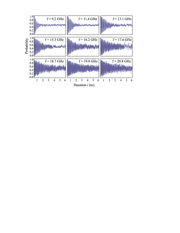
Figure 3: Some experimental oscillations observed for different pulse height. The measured frequency is indicated in the top right part of each plot.

Remarkably, changing the pulse height does not only modify the oscillation frequency but also influences qualitatively and quantitatively its decay law. This is more clearly pointed out considering the envelope of each probability, shown in figure 4. In contrast with the exponential decay typically originated from quantum noise, the decay of the probabilities are fitted by the decay law (blue lines in figure 4)[28]:

$$d(t)=\,\frac{1}{[1+(\gamma_{II}t)^{2}]^{1/4}}\,\exp{\left[-\frac{(\gamma_{I}t)^{2}}{2}\right]}\,,$$ (3)

with independent fitting parameters, $\gamma_{I}$ and $\gamma_{II}$.

Figure 4: Decay envelopes of the observed oscillations (red points), and relative fitting curves (blue continuous lines).

The combination of exponential quadratic and algebraic decay is characteristic of defocusing processes due to fluctuactions with $1/f$ spectrum of the parameters entering the splitting $\Omega$ [28, 29]. Similar behaviors have in fact been observed in different architectures and in the presence of microwave manipulation pulses [29]. The observed decay laws therefore suggest that the present experiment is mainly affected by $1/f$ noise in the control fluxes and in the junctions critical currents. Relaxation processes, typically leading to exponential decay, seem to be weakly effective.

The experimentally estimated values of $\gamma_{I}$ as a function of the frequency $f=f_{0}\sqrt{1+\beta(\varphi_{c})}$ ($f_{0}=\Omega_{0}/(2\pi)$) are reported in figure 5 (left panel - red dots). We observe a regular behavior characterized by a minimum at $f_{0}=\Omega_{0}/(2\pi)=19.8$GHz ($\varphi_{c}^{Top}\approx\pi$). This behavior suggests the existence of an optimal point in the present setup. The values of $\gamma_{II}$, shown in figure 5 (right panel - red dots) are instead quite scattered and we observe $\gamma_{II}>\gamma_{I}$, except for frequencies around $10$GHz where $\gamma_{II}\approx\gamma_{I}$. As a consequence, by changing the operating point, $\varphi_{c}^{Top}$, the probability turns from a decay approximately exponential to an algebraic behavior for frequencies $f$ close to $f_{0}$, where $\gamma_{I}$ is minimum.

In order to further understand whether this is the appropriate picture, in the following Section we theoretically analyze the effect of low and high frequency flux and critical current noise in the present setup. Before proceeding with the analysis, we need to identify the phases of the manipulation which are presumably more severely affected by noise sources. The various parts of the experiment can be addressed separately as follows:

1. Initial phase ”W”: During the initial ”W” phase, when the barrier is very high and the system is rigorously prepared in one of the two states, any possible transition between wells is blocked by the high barrier. The system remains in an eigenstate to high accuracy.

2. ”W-U-V” transition: The effect of noise during this rapid transition is a very difficult problem, involving an out-of-equilibrium dynamics. However, for the present experiment, noise during this phase is presumably irrelevant. In fact, any noise source acting during this transition should affect the oscillations amplitude independently on the pulse duration. Therefore we expect that it merely produces a net reduction of the visibility of the oscillation at the start time. Since we are able to observe oscillations with high visibilities, up to $95\%$ (fig.2), we conclude that the effect of noise during this phase is small. This fact can be tentatively explained by considering that the critical region where the change of the potential shape occurs (”U” region) is crossed over in a very short time (of the order of picoseconds), shorter than the typical time of coupling with the environment (few nanoseconds).

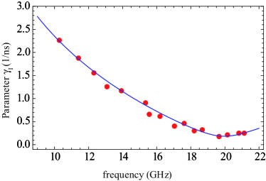
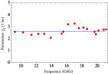
Figure 5: Red points are the decay rate $\gamma_{I}$ (left panel) and $\gamma_{II}$ (right panel) obtained by fitting of the experimental decay curves in figure 3 with eq. (3). The blue line in the left panel is the fit of the data points with eq. (10) (Section 3). In the right panel the blue line is the average value of the scattered values of $\gamma_{II}$

3. Phase ”V”: On the contrary, relaxation and decoherence will act heavily during the single well condition ”V”, with an effect depending on the time $t$ of permanence in this phase.

4. ”V-U-W” transition: For the return transition from the single to the double well potential (”V-U-W”) the same considerations of the ”W-U-V” transition hold (based on the initial visibility of the oscillation), so that one can conclude that also in this case the effect of noise is rather small.

5. Final phase ”W”: Finally, when the barrier is raised again in the final condition before the readout (”W”), transitions between the two wells are again blocked by the barrier. In this case the final state will be a superposition of the left/right states and the effect of dephasing can be quite strong. However, since we are just interested on the final population of one of the localized states, the information on the relative phase between the two states can be disregarded.

In conclusion, we expect that the observed decay of the probability can be attributed mainly to noise sources acting during the phase ”V”, when the system evolves during the time $t$ and several repetitions of the protocol are performed. In the following Section we will investigate the effect of low-frequency noise during repeated measurement protocols in the ”V” phase of the present experiment.

4 Defocusing during repeated measurements

Superconducting qubits in the various implementations are usually affected by broadband and non-monotonic noise [12, 29, 30]. The various noise sources responsible for this phenomenology have a qualitative different influence on the system evolution. To solve the qubit dissipative dynamics we apply the multi-stage elimination approach introduced in Ref. [28]. In simplest cases the effect of noise with large spectral components at low frequencies (adiabatic noise), like $1/f$ noise, and the effect of noise acting at frequencies of the order of the qubit splitting (quantum noise), can be treated independently. The leading effect of adiabatic noise during repeated measurement protocols is defocusing, analogous to inhomogeneous broadening in Nuclear Magnetic Resonance (NMR) [31]. It is expressed by the ”static path” or static noise approximation (SPA) describing the average of signals oscillating at randomly distributed effective frequencies [28, 29]. Defocusing can be sensitively reduced by operating at ”optimal points” where the variance of the stochastic frequency is minimal [32]. Quantum noise is instead responsible for relaxation processes. It can be treated by solving a Bloch-Redfield master equation, which leads to exponential decay with decoherence time denoted $T_{2}$ in the NMR notation [34].

The measurements reported in the previous Section indicate a dominant adiabatic noise. Here we concentrate our attention on the effect of noise during the single well ”V” phase, when the harmonic approximation holds with level spacing given in eq.(2). Defocusing originates from variations of the effective frequency $\Omega$ during the measurement runs which we attribute to fluctuations of the control bias fluxes $\delta\varphi_{x}$, $\delta\varphi_{c}$ and of the critical current $\delta I_{0}$, which correspond to fluctuations of $\beta_{0}$, $\delta\beta_{0}$. Fluctuations of the magnetic fluxes are caused by extrinsic and intrinsic sources. The electromagnetic circuit originates quantum noise. In addition, electric lines used to bias the qubit, in particular those coming from the room temperature electronics, are responsible for noise components mainly at low frequencies, where the filtering is weakly effective (below tens of kHz). The intrinsic flux noise acting on the superconducting loops is typically $1/f$ (adiabatic). Different models of flux noise microscopic sources have been proposed, like electron hopping between traps either with fixed randomly-oriented spins [35] or with spin flips [36]. Spin diffusion along the superconducting surface has also been proposed [37]. Fluctuations of the critical current are instead due only to intrinsic causes, like the presence of two state fluctuators in the junction barrier [38, 15]. In the present article, we do not address the important issue of the microscopic source of the fluctuations. Rather, we note the existence of low-frequency variations of the effective oscillation frequency and describe their effects in the adiabatic approximation. To this end we assume small fluctuations of $\Omega$ given in eq.(2) around the nominal values of the control parameters, $\varphi_{c}^{Top}$ and $\varphi_{x}=0$. The expansion of $\Omega$ to the second order in the fluctuations leads to $\Omega+\delta\Omega$ where

$$\frac{\delta\Omega}{\Omega_{0}}\sim b_{1}\,\delta\beta_{0}+c_{1}\,\delta\varphi_{c}-\frac{1}{2}\big{[}\,a_{2}\,\delta\varphi_{x}^{2}\,+\,b_{2}\,\delta\beta_{0}^{2}\,+\,c_{2}\,\delta\varphi_{c}^{2}\,+\,m_{2}\,\delta\varphi_{c}\delta\beta_{0}\,\big{]}\,.$$ (4)

The coefficients of the first and second order terms are (for semplicity here we use $\varphi_{c}$ for $\varphi_{c}^{Top}$)

$$b_{1}=\frac{1}{2}\frac{\cos(\varphi_{c}/2)}{\sqrt{1+\beta(\varphi_{c})}}\qquad\qquad\quad,\qquad\quad\quad\;\;c_{1}=-\frac{1}{4}\frac{\beta_{0}\sin(\varphi_{c}/2)}{\sqrt{1+\beta(\varphi_{c})}}$$ (5)

and

$$\!\!a_{2}=\frac{\beta(\varphi_{c})}{2(1+\beta(\varphi_{c}))^{5/2}}\quad\qquad \qquad\qquad b_{2}=\frac{\cos^{2}(\varphi_{c}/2)}{4(1+\beta(\varphi_{c}))^{3/2}}$$ , (6)

$$\!\!\!\!\!\!\!\!\!\!\!\!\!\!\!\!\!\!\!\!\!\!\!\!\!\!\!\!\!\!\!\!\!\!c_{2}=\frac{1}{8\sqrt{1+\beta(\varphi_{c})}}\left(\beta(\varphi_{c})+\frac{\beta_{0}^{2}\sin^{2}(\varphi_{c}/2)}{2(1+\beta(\varphi_{c}))}\right)\; \;m_{2}=\frac{\sin(\varphi_{c}/2)}{2(1+\beta(\varphi_{c}))^{3/2}}\left(1+\frac{\beta(\varphi_{c})}{2}\right).$$ , (7)

In the SPA the off-diagonal elements of the qubit reduced density matrix (RDM), $\rho(t)$, in the basis of the lowest eigenstates in the ”V” potential $\{|0\rangle,|1\rangle\}$ is obtained by evaluating the average over the fluctuations $\delta\varphi_{x}$, $\delta\varphi_{c}$ and $\delta_{\beta_{0}}$

$$\langle\rho_{01}(t)\rangle\,=\,\rho_{01}(0)\,e^{-i\Omega t}\,\langle e^{-i\delta\Omega t}\rangle\,,$$ (8)

here we assume that fluxes and critical current fluctuactions are are uncorrelated random variables with Gaussian distribution, zero mean and standard deviations $\sigma_{x}$, $\sigma_{c}$ and $\sigma_{\beta_{0}}$ respectively. We remark that for the fluctuations of the critical current this assumption should be checked considering the microscopic source of $I_{0}$ fluctuations. The power spectra of the control flux biases and of the critical current measured in similar flux or phase qubits reveal a $1/f$ behavior at low-frequencies [35, 38]. The variance of the corresponding variables, $\sigma_{\alpha}^{2}$ ($\alpha=x,c,\beta_{0}$), is proportional to the amplitude of the $1/f$ spectrum, $S_{\alpha}^{1/f}(\omega)=\pi\sigma_{\alpha}^{2}[\ln(\gamma_{M\alpha}/\gamma_{m\alpha})\,\omega]^{-1}$ ($\gamma_{m\alpha}$ and $\gamma_{M\alpha}$ are the low and the high frequency cut-offs of the $1/f$ region).
In order to compare with the experiments, we evaluate the average probability $\langle P_{LL}(t)\rangle$. For the chosen initial condition, $|\psi(t=0)\rangle=|L\rangle=(|0\rangle+|1\rangle)/\sqrt{2}$ the probability reads $\langle P_{LL}(t)\rangle=\frac{1}{2}+\langle{\rm Re}[\rho_{01}(t)]\rangle$. Where we assumed that the sum of the populations of the lowest eigenstates of the harmonic potential is constant, $\rho_{00}(t)+\rho_{11}(t)=1$. This assumption is justified in the adiabatic approximation, where populations do not evolve. It also holds in the presence of quantum noise, provided leakage from the bi-dimensional Hilbert space can be neglected.

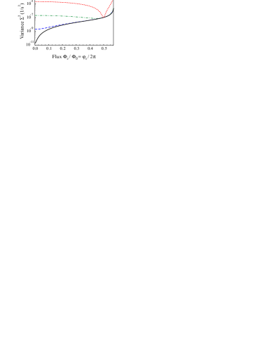
Figure 6: Variance of $\Omega$ given by eq. (13) as a function of $\varphi_{c}$ in the allowed interval of values where $\beta(\varphi_{c})>-1$ for $\sigma_{c}\sim\sigma_{x}\approx 3\times 10^{-4}$, and different $\sigma_{\beta_{0}}$ values $2\times 10^{-5}$, $2\times 10^{-4}$, $2\times 10^{-3}$, $2\times 10^{-2}$ from bottom to top.

The averaged probability thus reads

$$\langle P_{LL}(t)\rangle=\frac{1}{2}[1+\langle\cos((\Omega+\delta\Omega)t)\rangle]=\frac{1}{2}[1+d(t)\cos(\Omega t+\theta)]$$ (9)

where $d(t)=|\langle\exp{i\delta\Omega t}\rangle|$ and $\theta={\rm arg}[\langle\exp{i\delta\Omega t}\rangle]$. The coherence $\langle\rho_{01}(t)\rangle$ in the SPA is obtained evaluating the average eq.(8) with $\delta\Omega$ given by eq. (4). For short times (neglecting contributions $\propto t^{4}$ with respect to terms $\propto t^{2}$) $d(t)$ is indeed given by eq.(3) with $\gamma_{I}$ and $\gamma_{II}$ given by

$$\gamma_{I} = \Omega_{0}\sqrt{b_{1}^{2}\sigma_{\beta_{0}}^{2}+c_{1}^{2}\sigma_{c}^{2}}$$ (10)

$$\gamma_{II} = \Omega_{0}\sqrt{b_{2}^{2}\sigma_{\beta_{0}}^{4}+c_{2}^{2}\sigma_{c}^{4}+a_{2}^{2}\sigma_{x}^{4}+m_{2}^{2}\sigma_{\beta_{0}}^{2}\sigma_{c}^{2}}\,.$$ (11)

Note that the first order terms of the expansion (4) enter $\gamma_{I}$, the second order ones enter $\gamma_{II}$. Finally we include the possibility of incoherent energy exchanges with the environment due to quantum noise. In the simplest version of the multi-stage elimination approach the overall decay factor of the coherence is

$$d(t)=|\langle\exp{i\delta\Omega t}\rangle|\,e^{-t/T_{2}}\,,$$ (12)

where the decoherence time due to quantum noise, $T_{2}$, depends on the power spectrum of the flux and of the critical current fluctuations at frequency $\Omega$.

The existence of an optimal point in the present setup depends on the possibility to minimize the standard deviation of the effective splitting $\Omega$, $\Sigma=\sqrt{\langle\delta\Omega^{2}\rangle-\langle\delta\Omega\rangle^{2}}$ [32, 33]. In fact, from the short-times expansion of eq. (8) we find $|\langle e^{-i\delta\Omega t}\rangle|\approx\sqrt{1-(\Sigma t)^{2}}$, thus defocusing is reduced when $\Sigma$ is minimal. In the present case, from (4), we find

$$\Sigma^{2}=\gamma_{I}^{2}+\frac{1}{2}\gamma_{II}^{2}\,.$$ (13)

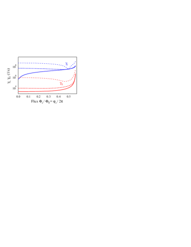
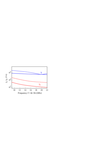
Figure 7: Left panel: $\gamma_{I}$ (blue) and $\gamma_{II}$ (red) as a function of $\varphi_{c}$ for $\sigma_{c}\sim\sigma_{x}\approx 3\times 10^{-4}$, and different $\sigma_{\beta_{0}}$ values (solid lines for $2\times 10^{-5}$, dashed lines for $2\times 10^{-3}$, dotted lines for $2\times 10^{-2}$). Right panel: $\gamma_{I}$ (blue) and $\gamma_{II}$ (red) as a function of $f=\Omega/2\pi$ in the experimental regime $\varphi_{c}\in[0.98\,\pi,1.2\,\pi]$ for the previous values of $\sigma_{c}$, $\sigma_{x}$ and $\sigma_{\beta_{0}}=2\times 10^{-5}$ (solid line), $\sigma_{\beta_{0}}=2\times 10^{-2}$ (dotted line).

Because of the periodicity of the first order terms in (4), included in the coefficients $b_{1}$ and $c_{1}$ defined in eq. (5), $\Sigma$ is mimimal either at $\varphi_{c}\approx 0$, when $\sigma_{c}>\sigma_{\beta_{0}}$, or at $\varphi_{c}\approx\pi$ in the opposite case. This is illustrated in figure 6 where we show $\Sigma$ for typical values of the variances $\sigma_{c}$ and $\sigma_{x}$ [35, 38] and increasing values of $\sigma_{\beta_{0}}$. Depending on which condition applies to a specific setup, the device can be operated at the proper optimal point .

The dependence of $\gamma_{I}$ and $\gamma_{II}$ on the operating point is reported in figure 7 for the same parameters of figure 6. In the considered regime, $\gamma_{I}$ is minimal at the optimal point, wherever it is located (left panel). This is a consequence of the fact that under these conditions the variance of $\Omega$ is dominated by the first order terms and $\Sigma\approx\gamma_{I}$. In the right panel of figure 7 we show $\gamma_{I}$ and $\gamma_{II}$ as a function of the frequency $f$ when $\varphi_{c}$ varies in the experimental range around $\varphi_{c}\approx\pi$ (as indicated in figure 2). In this frequency range $\gamma_{I}$ is minimal only when $\sigma_{\beta_{0}}>\sigma_{c}$ (corresponding to the dot-dashed and dotted curves in figure 6). We may thus expect that a similar situation occurs in the present experiment, with an optimal point at $\varphi_{c}^{Top}\approx\pi$ corresponding to a minimum of $\gamma_{I}$. However we note that for the parameters in figure 7, since $\gamma_{I}>\gamma_{II}$, the coherence decay $d(t)$ is dominated by the exponential factor $\exp{(\gamma_{I}^{2}t^{2}/2)}$, independently of the optimal point location. Since in the present experiment we observe a crossover from an exponential to an algebraic decay by changing the working point, for some operating conditions around $\varphi_{c}^{Top}\approx\pi$ it should turn out that $\gamma_{I}\lesssim\gamma_{II}$. Since at the considered working point ($\varphi_{x}=0$) fluctuactions of the flux $\varphi_{x}$ contribute to the second order in (4), the above relation between $\gamma_{I}$ and $\gamma_{II}$ may in principle occur when the flux variances differ considerably. Such a situation is hovewer unlikely, a dependence of $1/f$ flux noise on the SQUID size as due to a ”global magnetic field noise” has in fact been ruled out [35]. Such a situation is also excluded in the present experiment. An illustrative case with $\sigma_{x}\gg\sigma_{c}$ is shown in figure 8. Due to the increased weight of the second order terms in (4), $\gamma_{II}$ has a local mimimum at the optimal point, $\varphi_{c}^{Top}\approx\pi$. However for frequencies close to the minimum, being $\gamma_{II}<\gamma_{I}$, the decay factor would be exponential rather than algebraic, in contrast to the observations reported in the previous Section.

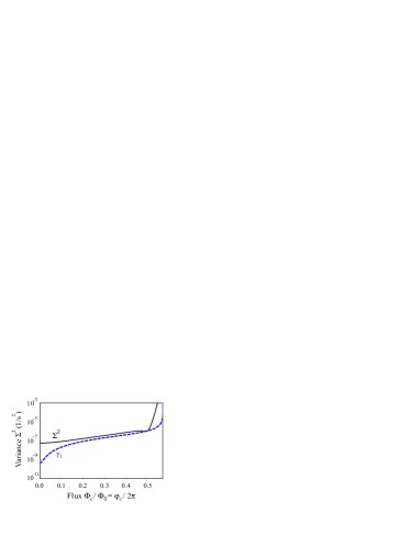
Figure 8: Left panel: variance $\Sigma^{2}$ as a function of $\varphi_{c}$ with the minimum at $\approx\pi$, continuous line is (13), the dashed line is the first order approximation $\Sigma\approx\gamma_{I}$. Right panel: the rates $\gamma_{I}$ and $\gamma_{II}$ as a function of $f$. The variances in this example have been fixed to highlight the regime $\gamma_{I}\gtrsim\gamma_{II}$, and are $\sigma_{c}\approx 10^{-3}$, $\sigma_{x}\approx 10^{-1}$, $\sigma_{\beta_{0}}\approx 10^{-4}$.

We conclude from this analysis that the present model, considering adiabatic fluctuations of the two fluxes $\varphi_{c}$ and $\varphi_{x}$, and of the critical current, predicts the existence of an optimal point of minimal variance of the effective splitting and of minimal $\gamma_{I}$, when first order terms in the expansion of the effective frequency $\Omega$ dominate. On the other side, it is difficult to predict the simultaneous existence of an optimal point at $\varphi_{c}^{Top}\approx\pi$ where $\gamma_{I}$ is minimum and $\gamma_{I}<\gamma_{II}$ only close to the minimum. A plausible scenario is that the present experiment is sensitive to first order contributions, entering $\gamma_{I}$, whereas second order effects entering $\gamma_{II}$ are masked possibly by additional noise sources not included in our analysis. For instance, our model does not include SQUID inductance fluctuactions with $1/f$ power spectrum, which are highly correlated to $1/f$ flux noise [39].

5 Fit of experimental data: $\gamma_{I}$, $\gamma_{II}$

According to the analysis of the previous Section, whereas for $\gamma_{I}$ we may expect an agreement between eq. (10) and experimental data, we expect that eq.(11) for $\gamma_{II}$ has to be supplemented by an additional contribution of different origin. Therefore, in order to extract $\gamma_{I}$, $\gamma_{II}$ and $1/T_{2}$ from the experimental data we fit the envelopes of the experimental curves in figure 3 considering them as independent parameters.

Indeed, the experimentally estimated $\gamma_{I}$ for the different oscillation frequencies $f$ can be fitted with eq.(10), giving a remarkable agreement with fitting parameters $\sigma_{c}=1.4\times 10^{-3}$ and $\sigma_{\beta_{0}}=0.105$, corresponding to $\sigma_{\Phi_{c}}=223\mu\Phi_{0}$ and $\sigma_{I_{0}}=1.7\,\mu$A, see figure 5 (left panel, blue line). The noise on the flux $\varphi_{c}$ in addition to the $1/f$ behavior, possibly is also influenced by low frequency noise components due to the room temperature instrumentation. For the estimated noise variances, fluctuations of the critical current are almost always dominating except for the optimal point at $f_{0}=\Omega_{0}/(2\pi)=19.8$GHz where the effect of flux noise emerges. The existence of this optimal point is evident from the decays in figure 4, where a crossover between two decay regimes is observed: a fast decay at lower frequencies is followed by a slower decay at higher frequencies.

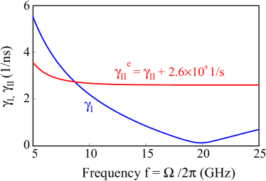
Figure 9: Plot of $\gamma_{I}$ (blue) and $\gamma_{II}^{e}=\gamma_{II}+2.6\cdot 10^{9}\,{\rm s}^{-1}$ (red) as a function of $f$ for variances extracted from the fit of $\gamma_{I}$, $\sigma_{c}\approx\sigma_{x}\approx 10^{-3}$, $\sigma_{\beta_{0}}\approx 10^{-1}$.

On the other side, the value of $\sigma_{\beta_{0}}$ obtained form the fit is much larger than the values reported in other superconducting qubits [35, 38]. An independent check of this quantity in the present setup is not possible, since measurements of the low-frequency power spectrum of critical current noise are not available at present. One possible explanation of the quite high value of $\sigma_{I_{0}}$ is related to the materials used for the qubit fabrication. In fact other superconducting qubits based on the same materials and fabrication technology and displaying coherence times similar to the ones reported in our experiment (few nanoseconds) [21] presented a considerable enhancement of these times by improving the used materials, for example by introducing $SiN_{x}$ dielectric films instead of standard $SiO_{2}$ for the crossover wiring [15, 16]. The full understanding of this point requires the repetition of the experiment with the use of different materials and technologies. Another possible source of this inconsistency stems from the assumed Gaussian distribution for the critical current fluctuations, $\delta\beta_{0}$. Evaluating possible deviations from the Gaussian approximation requires considering a microscopic model of critical current fluctuations. This is another possible extension of the present analysis.

The values of $\gamma_{II}$ extracted from the fit of the oscillations in figure 3 are scattered around an average value $\sim 2.6\cdot 10^{9}\,{\rm s}^{-1}$, as shown in figure 5. Equation (11) for $\gamma_{II}$ with $\sigma_{x}\sim\sigma_{c}=1.4\times 10^{-3}$ and $\sigma_{\beta_{0}}=0.105$ predicts $\gamma_{II}\ll\gamma_{I}$, in contrast with the observations. However, including a constant (frequency independent) noise contribution in the second order terms, i.e. defining an effective $\gamma_{II}^{e}\approx\gamma_{II}+2.6\cdot 10^{9}\,{\rm s}^{-1}$, the crossover from exponential to algebraic decay where $\gamma_{I}\ll\gamma_{II}$ visible in figure 5 can be quantitatively reconstructed, as illustrated in figure 9.

Finally, the reported measurements do not allow for a reliable estimate of the effect of quantum noise, included in the exponential decay term with $T_{2}$. The observations are compatible with a decoherence time $T_{2}$ with a lower limit of tens of nanoseconds, which is reasonable in this type of qubits [15].

6 Conclusions

In conclusion, we considered the manipulation of a double SQUID qubit by fast flux pulses, and observed the decay envelope of the obtained oscillations for different control conditions, corresponding to different oscillation frequencies. The shapes of the decay envelopes show a peculiar behaviour with a crossover between two distinct regimes. These behaviors can be attributed to various sources of adiabatic noise affecting the system. The effect of high frequency noise is negligible, and this indicates a correct filtering and shielding of the system.

We observed a crossover between an exponential and an algebraic decay regime, with an optimal point where decay is algebraic. We demonstrated that this behavior is due to the interplay of first order effects of low-frequency flux and critical current noise. In general, intrinsic fluctuation of the critical current dominate except at the optimal point where the weaker effect of flux bias fluctuations springs up. The existence of the optimal point is an interesting characteristic for possible applications.

The effect of second order fluctuating terms is still misunderstood and will require further investigation. To this end we plan to repeat the experiment with different, improved materials. The ensuing noise characterization may possibly provide new insights into the low-frequency noise sources in this kind of setup.

References

References

- [1] Ladd T D et al2010 Nature 464 45-53.
- [2] Clarke J and Wilhelm F K 2008 Nature 453 1031-1042.
- [3] Devoret M H and Martinis J M 2004 Quantum Information Processing 3 163-203.
- [4] Majer J et al2007 Nature 449 443-447.
- [5] DiCarlo L et al2009 Nature 460 240-244.
- [6] Manucharyan V E et al2009 Science 326 113-116.
- [7] Johnson B R et al2010 Nature Physics 6 663-667.
- [8] A. Palacios-Laloy A et al2010 Nat. Phys. 6, 442-447.
- [9] Ansmann M et al2009 Nature 461 504-506.
- [10] Hofheinz M et al2008 Nature 454 310-314.
- [11] Nakamura Yet al1999 Nature 398 786; Yu Y et al2002 Science 296 889; Martinis J M et al2002 Phys. Rev. Lett.89 117901; Chiorescu I et alScience 299 1869; Yamamoto T et alNature 425 941; Saito S et al2004 Phys. Rev. Lett.93 037001.
- [12] Vion D et al2002 Science 296 886.
- [13] Yoshihara F et al2006 Phys. Rev. Lett.97 167001.
- [14] Blais A et al2004 Phys. Rev. A 69 062320; Devoret M H et alet al. in Quantum Tunneling in Condensed Media (eds Kagan, Y. and Leggett, A. J.) 313 - 345 (Elsevier, Amsterdam, 1992); Wallraff A et al2004 Nature 431 162 - 167.
- [15] Martinis J M et al2004 Phys. Rev. Lett. 95, 210503.
- [16] McDermott R, 2009 IEEE Transactions on Applied Superconductivity 19, 2-13.
- [17] Carelli P et al2001, Ieee Transactions on Applied Superconductivity 11, 210-214.
- [18] Chiarello F 2000 Physics Letters A 277, 189-193.
- [19] Castellano M G et al2010 New J. Phys. 12, 043047.
- [20] Poletto S et al2009 New J. Phys. 11, 013009.
- [21] Poletto S et al2009 Physica Scripta T137, 014011.
- [22] Castellano M G et al2007 Phys. Rev. Lett. 98, 177002.
- [23] Chiarello F 2007 The European Physical Journal B - Condensed Matter and Complex Systems 55, 7-11.
- [24] A. B. Zorin and F. Chiarello 2009 Phys. Rev. B 80, 214535.
- [25] Castellano M G et al2003 Journal of Applied Physics 94, 7935-7937.
- [26] Zorin A B 1995 Rev. Sci. Instrum. 66, 4296.
- [27] Steffen M et al2010 J. Phys.: Condens. Matter 22, 053201.
- [28] Falci G et al2005 Phys. Rev. Lett. 94, 167002.
- [29] Ithier G et al2005 Physical Review B 72 134519.
- [30] Astafiev O et al2004 Phys. Rev. Lett. 93, 267007.
- [31] Schlichter C P , Principles of Magnetic Resonance (Springer, New York, 1996).
- [32] Paladino E et al2010 Phys. Rev. B 81, 052502.
- [33] Paladino E et al2011 New J. Phys. 13 093037.
- [34] C. Cohen-Tannoudji, J. Dupont-Roc and G. Grynberg, Atom-Photon Interactions, Wiley-Interscience (1993).
- [35] Koch R H et al2007 Phys. Rev. Lett. 98 267003.
- [36] de Sousa R 2007 Phys. Rev. B 76 245306.
- [37] Faoro L and Ioffe L B 2008 Phys. Rev. Lett. 100 227005.
- [38] Van Harlingen D J et al2004 Phys. Rev. B 70 064517.
- [39] Sendelbach S et al2009 Phys. Rev. Lett. 103, 117001.