METHODS TO COMPUTE PRESSURE AND WALL TENSION IN FLUIDS CONTAINING HARD PARTICLES

Abstract

Colloidal systems are often modelled as fluids of hard particles (possibly with an additional soft attraction, e.g. caused by polymers also contained in the suspension). In simulations of such systems, the virial theorem cannot be straightforwardly applied to obtain the components of the pressure tensor. In systems confined by walls, it is hence also not straightforward to extract the excess energy due to the wall (the “wall tension”) from the pressure tensor anisotropy. A comparative evaluation of several methods to circumvent this problem is presented, using as examples fluids of hard spheres and the Asakura-Oosawa model of colloid-polymer mixtures with a size ratio $q=0.15$ (for which the effect of the polymers can be integrated out to yield an effective attractive potential between the colloids). Factors limiting the accuracy of the various methods are carefully discussed, and controlling these factors very good mutual agreement between the various methods is found.

PACS numbers: 82.70.Dd, 05.10.Ln, 61.20.Ja, 68.08.-p

1 Introduction

In many colloidal dispersions, the interaction between the colloidal particles (or at least the repulsive part of these interactions) can be represented as that of hard particles (hard spheres, hard rods, etc.) [1, 2, 3, 4, 5]. Colloidal dispersions are model systems for the experimental study of cooperative phenomena in condensed matter, since the size of these particles (in the $\mu m$ range) and their slow dynamics allows their study in unprecedented detail, which would not be possible for condensed matter systems formed from small molecules. Moreover, hard particles are the archetypical many-body systems, for which computer simulation methods were first introduced a long time ago: the importance sampling Monte Carlo method [6] was introduced discussing a fluid of hard disks; similarly, Molecular Dynamic methods were introduced in the context of the study of the hard sphere fluid [7]. These fluids formed from hard particles also are an important testing ground for analytical theories of fluids [8]. The above remarks just sketch a few motivations to explain why the simulation of fluids formed from hard particles is of fundamental importance.

However, simulations of fluids containing hard particles suffer from one important technical difficulty: the well-known virial equation for the pressure tensor (for systems where particles interact with pair-wise forces $\vec{f}(\vec{r}_{ij})$ with $r_{ij}=|\vec{r}_{ij}|,\vec{r}_{ij}=\vec{r}_{i}-\vec{r}_{j})$ [8]

$$p^{\alpha\beta}=\rho k_{B}T\,\delta^{\alpha\beta}+\frac{1}{dV}\Big{\langle}\sum\limits_{i<j}f^{\alpha}(\vec{r}_{ij})r^{\beta}_{ij}\Big{\rangle}_{NVT}$$ (1)

is not straightforwardly applicable (for hard spheres of diameters $\sigma_{i}$, the force $\vec{f}\equiv 0$ if $r_{ij}>(\sigma_{i}+\sigma_{j})/2$, while distances $r_{ij}<(\sigma_{i}+\sigma_{j})/2$ are excluded, and for $r_{ij}=(\sigma_{i}+\sigma_{j})/2$ the potential energy jumps from zero to infinity, and hence the force is also not defined in this case). Note that in Eq. (1) $\alpha,\beta$ denote Cartesian components, $\rho=N/V$ is the density ($N$=particle number, $V$= “volume” of the $d$-dimensional system), $k_{B}$ is Boltzmann’s constant, $T$ absolute temperature, and $\langle\cdots\rangle_{NVT}$ is understood as a statistical average in the canonical ($NVT)$ ensemble. Computation of the pressure is not only of the interest to clarify the equation of state of the considered system in the bulk, but is also required when one considers a system confined by walls, and wishes to estimate the excess free energy due to the walls. Assuming a geometry where the system is confined by two identical walls at a (large) distance $D$ apart, the wall-fluid surface excess free energy per unit area $\gamma_{wf}$ (also called “wall tension”) is expressed in terms of the anisotropy of the pressure tensor as [9]

$$\gamma_{wf}=D(P_{N}-P_{T})/2$$ (2)

where $P_{N}=p^{zz}$ is the “normal pressure” which in equilibrium is homogeneous in the system, while $P_{T}$ is the average tangential pressure

$$P_{T}=(1/2D)\int\limits_{0}^{D}(p^{xx}(z)+p^{yy}(z))dz.$$ (3)

Note that Eq. (2) supposes that the two walls are far enough from each other that in between the fluid can attain its bulk properties, i.e. the two walls are non-interacting, the density profile $\rho(z)$ as well as the transverse pressure tensor components $p^{xx}(z)$ and $p^{yy}(z)$ are constant, independent of $z$, for a broad region of $z$ near $z=D/2$. In contrast, $\rho(z)$ does depend on $z$ near the walls, as well as $p^{xx}(z)$ and $p^{yy}(z)$, while the transverse component $p^{zz}(z)$ is strictly independent of $z$, irrespective of the choice of $D$. The generalization of $p^{\alpha\beta}$ in Eq. 1, which addresses only the behavior in the bulk, to such inhomogeneous systems with external boundaries will be discussed in Sec. 3 below.

In the present paper, we shall discuss methods from which the pressure and the wall tension can be computed for fluids where particles experience hard-core interactions, and hence the straightforward use of Eq. 1, or its extension to inhomogeneous systems is not possible. In Sec. 2, we shall describe the application of a recent method due to Schilling and Schmid [10], to compute absolute free energies of disordered structures by molecular simulations, considering the situation described above, where a system is confined by walls. We assume planar, structureless walls, with a smooth repulsion described by a Weeks-Chandler-Andersen (WCA) [11]-type potential,

$$V_{\rm WCA}(z)=4\varepsilon[(\sigma_{w}/z)^{12}-(\sigma_{w}/z)^{6}+1/4],\,0\leq z\leq z_{c}=\sigma_{w}2^{1/6}\quad,$$ (4)

while $V_{WCA}(z\geq z_{c})=0$. Here the strength ($\varepsilon$) and range $(\sigma_{w})$ of the potential provide parameters which can be varied, and so also the wall tension $\gamma_{wf}$ can be changed. For the chosen geometry, the free energy density can be written as

$$f(\rho,T,D)=f_{b}(\rho,T)+(2/D)\gamma_{wf}$$ (5)

where $f_{b}(\rho,T)$ is the free energy density of a corresponding bulk system at density $\rho$ and temperature $T$. We shall test the applicability of Eq. (5) for the simplest case, namely the hard sphere fluid.

In Sec. 3 we follow the alternative approach of De Miguel and Jackson [12], where Eqs. (2), (3) are used for hard particles in spite of the fact that a straightforward use of Eq. (1) is not possible. In this method, virtual changes of simulation box linear dimensions are performed to sample the probability that no molecular pair overlaps would occur as a result of these virtual moves. From this probability, the pressure can be estimated. While we already have verified the accuracy of this method for the case of a hard sphere fluid [13], we here extend the method to the case where the interparticle potential has both a hard core repulsion and a soft attraction. A well-known and practically relevant example for such a situation is provided by the Asakura-Oosawa model [14, 15, 16] for colloid-polymer mixtures, in the limit where the polymers are much smaller than the colloids. Describing the colloids as hard spheres of diameter $\sigma$ and the polymers as soft spheres of diameter $\sigma_{p}$, polymer-colloid overlap is also strictly forbidden, but polymer coils can interpenetrate and hence overlap with negligible energy cost. For $q\equiv\sigma_{p}/\sigma\leq 0.154$, one can integrate out the polymer degrees of freedom from the partition function exactly, replacing their physical effects by an effective attractive interaction between the colloids [14, 15, 16, 17, 18]

$$V_{\rm AO}(r)/k_{B}T=-\eta^{r}_{p}\Big{(}\frac{1+q}{q}\Big{)}^{3}\Big{\{}1-\frac{3r/\sigma}{2(1+q)}+\frac{(r/\sigma)^{3}}{2(1+q)^{3}}\Big{\}},\quad\sigma<r<\sigma+\sigma_{p},$$ (6)

while $V_{\rm AO}(r<\sigma)=\infty$, $V_{AO}(r\geq\sigma+\sigma_{p})=0$. The strength of this attractive potential is controlled by the “polymer reservoir packing fraction” $\eta_{p}^{r}$, which is related to the chemical potential $\mu_{p}$ of the polymers as $\eta^{r}_{p}=(\pi/6)\sigma^{3}_{p}\exp(\mu_{p}/k_{B}T)$.

Both methods of Secs 2. and 3 are checked by applying an independent third method, extending [13] a thermodynamic integration method [19] where one gradually inserts a wall potential in a system without walls (with periodic boundary conditions). Our extension [13] called “ensemble mixing method“ samples the free energy of systems with intermediate Hamiltonians. This new method is presented in Sec. 4, while Sec. 5 presents our conclusions.

2 Estimation of wall tension from computation of absolute free energies

As is well known, the absolute free energy of a system is normally not a straightforward output of a Monte Carlo simulation [20]. The most commonly used strategy is to use thermodynamic integration, supposing that the Hamiltonian $\mathcal{H}(\lambda)$ depends on a parameter $\lambda$ that can be varied from a reference state (characterized by $\lambda_{0}$) whose free energy is known, to the state of interest ($\lambda_{1}$), without crossing any phase transition,

$$\Delta F=F(\lambda_{1})-F(\lambda_{0})=\int\limits_{\lambda_{0}}^{\lambda_{1}}d\lambda^{\prime}\langle\mathcal{H}(\lambda^{\prime})/\partial\lambda^{\prime}\rangle_{\lambda^{\prime}}\quad.$$ (7)

For a dense fluid, Schilling and Schmid [10] propose to take as a reference state a configuration that is representative for the structure of interest (obtained within a standard simulation of the considered system). From this well-equilibrated state a reference state is constructed by fixing this particular configuration with suitable external potentials that hold all particles rigidly in their position $\{\vec{r}^{\;p}_{i}\}$ in that particular configuration (and the internal interactions between the particles can be switched off). In practice, Schilling and Schmid [10] used as a pinning potential in the reference state

$$U_{\rm ref}(\lambda)=\lambda\sum_{i}\phi(|\vec{r}_{i}-\vec{r}_{i}^{\;p}|/r_{\rm cut}),\,\,{\rm with}\,\phi(x)=x-1\,,$$ (8)

where it is understood that particle $i$ can only be pinned by well $i$ at $\vec{r}_{i}^{\;p}$, and not by the other wells (but one carries out identity swaps to make the particles indistinguishable). For this non-interacting reference state the (configurational) reference free energy is

$$F_{\rm ref}(\lambda)=\ln(N/V)-\ln[1+(V_{0}/V)g_{\phi}(\lambda)]\quad,$$ (9)

where $V_{0}=4\pi r^{3}_{\rm cut}/3$ and $g_{\phi}(\lambda)=3\lambda^{d}(e^{\lambda}-\sum\limits_{k=0}^{3}e^{k}/k!)$, for the above choice of $\phi(x)$. Then, intermediate models are defined as

$$\mathcal{H}^{\prime}(\lambda)=\mathcal{H}_{\rm int}+U_{\rm ref}(\lambda)\quad,$$ (10)

where $\mathcal{H}_{\rm int}$ describes the interactions in the system which then are switched on (if necessary, in several steps). The free energy difference relative to $F_{\rm ref}(\lambda)$ then is computed by thermodynamic integration, for which $\langle\partial\mathcal{H}_{\rm ref}(\lambda)/\partial\lambda\rangle=\langle\sum_{i}\phi(|\vec{r}_{i}-\vec{r}_{i}^{\;p}|/r_{\rm cut})\rangle_{\lambda}$ needs to be sampled. For details, how this is done efficiently, we refer to the original publication [10]. Schilling and Schmid [10] have already tested this method for hard spheres in the bulk, obtaining the free energy for several densities, and verifying the (expected) agreement with the Carnahan-Starling equation of state [21].

In the present section, we present a straightforward extension of this method to a hard sphere system in a $L\times L\times D$ geometry, choosing $L=6$ (lengths being measured in units of $\sigma$), choosing a packing fraction $\eta=(\pi/6)\rho=0.3686$ and several choices for $D$ (Fig. 1). In order to obtain a reliable estimation of the error of this method, the approach was repeated for each choice of $D$ for 5 independent (but equivalent) reference configurations. The total number of Monte Carlo steps per particle for each of these runs was in the order of about $4\cdot 10^{5}$ for each of the $500$ steps of the thermodynamic integration and about $2\cdot 10^{6}$ for each of the $40$ steps in which the potential wells were switched on. Fig. 1 shows that indeed $F/D$ plotted vs. $1/D$ is compatible with a straight line, and the intercept of this straight line agrees with the Carnahan-Starling result (which was verified directly by also running a $L\times L\times L$ system at the chosen packing fraction). The accuracy with which the straight line can be fitted to the data points allows us to estimate $\gamma_{wf}$ from Eq. (5) with a relative accuracy of about 1%, and the result (choosing units such that $k_{B}T=1$) $\gamma=1.01\pm 0.01$ is fully compatible with the result of the ensemble mixing method for this case (Sec. 5). Thus, Fig. 1 is a valuable feasibility test that shows that the Schilling-Schmid method [10] is useful for the estimation of interfacial excess free energies of fluids.

3 Computation of the pressure tensor in systems of hard particles confined by walls

In this section we consider the AO-model of colloid-polymer mixtures, where particles interact both with a hard core interaction (for $r<\sigma)$ and a soft attractive part of the interaction, as described in Eq. (6). We wish to apply Eq. (2), and need to compute both $P_{N}$ and $P_{T}$ for this purpose. Furthermore we allow again for walls where the WCA potential, Eq. (4), acts.

First we note that in a system which is inhomogeneous in the $z$-direction the generalization of Eq. (1) to a local pressure tensor can be written as [22]

$$p^{\alpha\beta}(z)=\rho(z)k_{B}T\delta^{\alpha\beta}-\frac{1}{L^{2}}\sum\limits_{i<j}r^{\alpha}_{ij}\Big{(}\frac{\partial U}{\partial\vec{r}_{ij}}\Big{)}^{\beta}\theta[(z-z_{i})/z_{ij}]\theta[(z_{j}-z)/z_{ij}]/{|z_{ij}|}$$

$$-\rho(z)z\frac{d}{dz}V_{\rm WCA}(z)\delta^{\alpha z}\delta^{\beta z}\quad.$$ (11)

Note that in the total force acting on a particle there is also a contribution due to the wall potential, which has been written down explicitly in the last term, which contributes only for $\alpha=z$ and $\beta=z$. Thus, we can decompose $p^{zz}$ into the three contributions $\rho(z)k_{B}T$ and $p_{\rm wall}(z)\equiv-\rho(z)z(dV_{\rm WCA}(z)/dz)$ and the part due to interparticle interaction $p^{zz}_{\rm int}(z)$,

$$p^{zz}=\rho(z)k_{B}T+p^{zz}_{\rm int}(z)+p_{\rm wall}(z)\quad,$$ (12)

noting that while all three components of $p^{zz}$ do have a pronounced $z$-dependence in Eq. (12), the total normal pressure $p^{zz}$ in fact must be independent of $z$.

In our case Eqs. (3), (12) can be applied directly with respect to the soft attractive part of the interactions, but not with respect to the hard core part. Here we apply the principle that all contributions to the pressure simply are additive,

$$p^{\alpha\beta}_{\rm int}(z)=p^{\alpha\beta}_{\rm int,\,soft}(z)+p^{\alpha\beta}_{\rm int,\,hard}(z)\quad,$$ (13)

and we only compute $p^{\alpha\beta}_{\rm int,\,soft}(z)$ directly from the virial expression, i.e. the second term on the right hand side of Eq. (3), while for $p^{\alpha\beta}_{\rm int,\,hard}(z)$ we apply the method of De Miguel and Jackson [12], as already used in our previous work on the hard sphere fluid [13].

In the latter method, one considers virtual volume changes according to

$$D\rightarrow D^{\prime}=D(1-\xi),\,L\rightarrow L^{\prime}=L(1-\xi)$$ (14)

where $\xi<<1$. In any equilibrium configuration, there cannot be any overlaps between the hard cores of any pair of particles, but in dense fluids these virtual moves will create some overlaps. One then can sample the probabability $P_{\rm nov}(\xi)=\exp(-b\xi)\approx 1-b\xi$ that no overlap of particles occurs. Denoting the constant $b$ for the moves from $D$ to $D^{\prime}$ as $b_{N}$, and for moves from $L$ to $L^{\prime}$ as $b_{T}$, we obtain

$$P_{N,\,{\rm hard}}/(\rho k_{B}T)=1+b_{N}/N,$$ (15)

$$P_{T,\,{\rm hard}}/(\rho k_{B}T)=1+b_{T}/N\quad,$$ (16)

where

$$P_{N,{\rm hard}}=(1/D)\int\limits_{0}^{D}p^{zz}_{\rm int,\,hard}(z)dz\quad,$$ (17)

and

$$P_{T,\,{\rm hard}}=(1/2D)\int\limits^{D}_{0}[p^{xx}_{\rm int,\,hard}(z)+p^{yy}_{\rm int,\,hard}(z)]dz.\quad.$$ (18)

In view of the substantial difficulty in obtaining very accurate simulation “data”, we have not attempted to compute the individual profiles $p^{\alpha\beta}_{\rm int}(z)$, noting that for the desired use of Eq. (2) only the quantities averaged across the film matter, as written in Eqs. (17), (18).

As an example, Fig. 2 shows the density profile $\rho(z)$ and the profile $p_{\rm wall}(z)$ as well as the profiles of those parts of both $p^{zz}_{\rm int}(z)$ and $p_{\rm int}^{xx}(z)=p^{yy}_{\rm int}(z)$ that are due to attractive parts of the potential of the AO model (Eq. 6). We recognize that all these contributions exhibit rapid large oscillations near the walls. These oscillations need to be well resolved (with a binning of the $z$-coordinate that is about an order of magnitude smaller than the hard sphere diameter, which sets the scale for these oscillations) and carefully sampled. Otherwise systematic errors are made when these contributions are integrated over $z$, and despite of the simplification that only integrated pressures are needed (cf. Eqs. (17), (18)) all results would suffer from systematic errors.

However, even with this simplification it is very difficult to obtain a very good accuracy, because systematic errors that occur if the range of $\xi$ for which $P_{\rm nov}(\xi)$ is sampled are not extremely small.

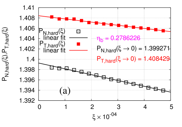
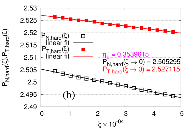
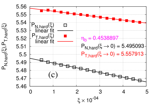
Figure 3: Extrapolation of the repulsive part of the total normal pressure $P_{N,{\rm hard}}$ and the total tangential pressure $P_{T,{\rm hard}}$ resulting from the hard sphere interactions at three packing fractions plotted vs $\xi$ for $\eta_{b}=0.2786226$(a), $0.3539615$(b) and $0.4538897$(c).

For the sampling of $P_{\rm nov}(\xi)$, a careful sampling of the probability that pairs of particles occur at a distance $\sigma+\Delta r$ from each other is required, for very small values of $\Delta r$ is required. Of course, the number of particles $n(\Delta r)$ that occur at a distance in between $\sigma$ and $\sigma+\Delta r$ goes to zero as $\Delta r\rightarrow 0$. The constants $b_{N}$ and $b_{T}$ in Eqs. (15), (16), as well as the analogous constant for the bulk pressure in a system with periodic boundary conditions, depend very sensitively on the magnitude of $\xi$ that is considered in the virtual volume changes considered in Eq. (14), or, equivalently, the range of $\Delta r$ that is used to fit the derivative of $dn(\Delta r)/d(\Delta r)$ as $\Delta r\rightarrow 0$. This problem is illustrated in Fig. 3 for several cases of $\eta_{b}$. Note that the range of $\xi$ from $0<\xi<5\cdot 10^{-4}$ must be probed to allow an accurate linear fit from which the limiting value for $\xi\rightarrow 0$ can be extracted. If one fits a larger range of $\xi$, systematic errors do arise, particularly for larger values of the packing fraction. Note also that the relative range of pressure variation with $\xi$ increases with increasing packing fraction. Thus, it is rather easy to find a correct result for rather small values of the bulk packing fraction $\eta_{b}$, but much more difficult when $\eta_{b}$ approaches the region where the onset of crystallization occurs. This problem is not specific for the AO model, but occurs for the pure hard sphere system as well. In fact, already an examination of the local density near the walls (Fig. 4) shows that in the fluid phase both models are still very similar (only the solid phases at the liquid to solid transition have rather different packing fractions [23], and the interfacial stiffness between the coexisting phases also differ appreciably [23]). In the AO model, the first peak of the layering structure near the WCA wall is slightly higher and slightly sharper as in the pure hard sphere case, but otherwise the differences are rather minor.

Fig. 5 then presents the various contributions to the pressure as well as the wall tension $\gamma_{wf}$ as a function of bulk packing fraction. Of course, for the application of Eq. (2) the individual terms $P_{N}$, $P_{T}$ need to be obtained with an accuracy much better than one part in a thousand, if for large $D$ a meaningful accuracy of $\gamma_{wf}$ is desired: From Fig. 5(a), we recognize that near the crystallization transition (which occurs for [23] $\eta_{p}=0.494)$ the pressure in the bulk is of order 10¹, while $\gamma_{wf}$ is of order 10^o. With $D/2$ of order 20, Eq. (2) implies $P_{N}-P_{T}$ is of order $1/20$, and hence $(P_{N}-P_{T})/P_{N}$ is of order 1/200. This consideration already explains why (on the scale of Fig. 5a) the difference between $P_{N}$ and $P_{T}$ is invisible, and getting $\gamma_{wf}$ accurate to a few percent hence is a computational tour de force. This consideration explains readily why already for the case of hard spheres it has happened that different methods for the estimation of $\gamma_{wf}$ have yielded results that slightly different from each other (see Ref.  [13] for a recent account on the literature of this problem).

4 The ensemble mixing method

In Ref. [13] we have already presented very briefly the ensemble mixing method where one gradually transforms from a system without walls in the (NVT) ensemble (with periodic boundary conditions in all three space directions) to a system with two parallel walls at distance $D$ from each other (and periodic boundary conditions only in the $x,y$ directions parallel to the walls). Describing the system without walls by a Hamiltonian $\mathcal{H}_{1}(\vec{X})$, $\vec{X}$ denoting a point in configuration space, and the system with walls by $\mathcal{H}_{2}(\vec{X})$, the idea (originally proposed by Heni and Löwen [19]) is to construct a smooth path along which one can carry out a thermodynamic integration, that yields the free energy difference between the two systems, from which hence $\gamma_{wf}$ can be inferred. Heni and Löwen [19] applied this idea to the fluid of hard spheres, and also the recent extension due to Deb et al. [13] deals with the hard sphere fluid only. In the present section, we demonstrate that this method can equally well be applied to the AO model.

Since both systems $\mathcal{H}_{1}(\vec{X})$ and $\mathcal{H}_{2}(\vec{X})$ refer to the same choice of particle number $N$ and volume $V$, i.e. the same phase space, one can think of constructing an interpolation Hamiltonian $\mathcal{H}(\vec{X})$ as follows,

$$\mathcal{H}(\vec{X})=(1-\kappa)\mathcal{H}_{1}(\vec{X})+\kappa\mathcal{H}_{2}(\vec{X})$$ (19)

where the parameter $\kappa\in[0,1]$ is varied for calculating the free energy difference between the systems $(1,2)$. In our simulations, $\kappa$ is discretized in a set of discrete values $\{\kappa_{i}\}$, and the system is allowed to jump from $\kappa_{i}$ to a neighboring value, $\kappa_{i+1}$ or $\kappa_{i-1}$. These moves are accepted or rejected with a Metropolis step, and hence in order to ensure a large enough acceptance probability, the number of intermediate systems $\{\kappa_{i}\}$ needs to be chosen proportional to the volume $V$ of the system. We sample the relative probability $P(i)$ to reside in state $i$ with a variant of Wang-Landau sampling [24, 25]. Alternatively, other free-energy schemes like successive umbrella sampling can be applied[26]. The free energy difference between the two states $i$ and $i+1$ is given by $k_{B}T[\ln P(i)-\ln P(i+1)]$. In this way one can sample the free energy difference $\Delta F(D)$ for any given choice of $D$, between a system with walls and the system of corresponding thickness and particle number but without walls. The wall free energy then follows as

$$\gamma_{wf}=\lim\limits_{D\rightarrow\infty}\Delta F(D)/(2L^{2}k_{B}T)\quad.$$ (20)

Note that due to the excess density $\rho_{s}$ at the walls (which is present in the systems with walls, so that $\rho=N/V=\rho_{b}+(2/D)\rho_{s}$), for any finite $D$ the bulk density of the system with periodic boundary conditions (which is $\rho$) differs slightly but systematically from the bulk density in the system with the walls (which is $\rho_{b}=\rho-(2/D)\rho_{s})$. This fact already suggests that the extrapolation in Eq. (20) should be carried out in terms of a plot of $\Delta F(D)/(2L^{2}k_{B}T)$ linearly versus $1/D$ (Fig. 6). In this way the data included already in Fig. 5(b) have been generated.

Of course, in this method the lateral linear dimension $(L=8.05\sigma)$ is rather small, and often even smaller choices for $L$ have been used (e.g., $L=5\sigma)$ [13]. However, no significant finite size effects associated with the use of such small values of $L$ were detected. For the pressure tensor calculations, somewhat larger choices for $L$ have been possible (near $L=12$). Again, the good agreement between both methods to obtain $\gamma_{wf}$ for a significant range of $\eta_{b}$ (Fig. 5b) can be taken as an indication that neither method suffers from significant systematic errors, in the range of the parameters of interest for the present model.

5 Conclusion

In this paper, a comparative study of several methods to compute the excess free energy of walls in fluids (the “fluid-wall tension”) has been presented, considering fluids where the particles exhibit a hard-core repulsion, and hence the standard method based on the wall-induced anisotropy of the pressure tensor is not straightforward to apply. We have described three methods: (i) In the Schmid-Schilling method, the absolute free energy of the system is computed. When one does this for systems in a film geometry with several choices for the distance $D$ between the walls confining the film, one can infer the wall tension $\gamma_{wf}$ from the coefficient of the term in the free energy that exhibits a $1/D$ variation. We have tested this method so far for the hard sphere fluid only, but we did find good agreement with other methods. (ii) The pressure tensor anisotropy method can in fact be generalized to systems, with hard potentials, by a careful sampling of the probability $P_{\rm nov}(\xi)$ that particles do not overlap when virtual changes of the linear dimensions by a factor $1-\xi$ are performed. We have applied this method to the AO model of a colloid-polymer mixture, where the (implicitly treated) polymers are responsible for an effective attraction between the particles. The latter part of the potential is treated via the virial formula for the pressure tensor, while the repulsive part is treated with a sampling of $P_{\rm nov}(\xi)$, as mentioned above. We have shown that by a careful consideration of accuracy issues this method does yield valid results, but a substantial computational effort is needed. (iii) The third method is the ensemble mixing method, where one considers systems with periodic boundary conditions and no walls “mixed” (in the sense of a combined Hamiltonian, Eq. (19)) with a system with the same particle number and linear dimensions, but bounded by walls. This method has been used to test the other two methods, and our practical experience is that this last method amounts to the relatively smallest computational effort, in comparison with the other two methods. In the future work, we plan to use such methods to study the wetting behavior of colloidal dispersions.

Acknowledgement: This work was supported by Deutsche Forschungsgemeinschaft (DFG) under grants No Bi 314/19 (D.D.), TR6/C4 (D.W.) and TR6/A5 (A.W.). We are grateful to NIC Jülich for a generous grant of computer time at the JUROPA supercomputer of the JSC. It is a pleasure to dedicate this paper to David P. Landau on occasion of his 70^th birthday, and to thank him for his inspiring work over many decades, which also has been instrumental for some of the developments described here (in particular, the ensemble mixing method has profited from the Wang-Landau algorithm).

file=fig1.pdf,width=6.7cm

Figure 1: Extrapolation of the free energy $f(\eta_{c},D)$ of a hard sphere system at a packing fraction $\eta_{c}=0.3686$ of colloids plotted versus $2/D$, $D$ being the distance between two parallel walls, at which the WCA potential (Eq. (4)) acts. Note that the intercept at the ordinate is known accurately from the Carnahan-Starling equation of state. The slope of the straight line fit yields the wall tension.

$\begin{array}[]{ccc}\includegraphics[width=216.81pt]{fig2a_inset.pdf}&&\includegraphics[width=216.81pt]{fig2b_inset.pdf}\end{array}$

Figure 2: Profiles of the packing fraction $\eta(z)$ and wall contribution $p^{zz}_{\rm soft}(z)$ to the normal pressure $p_{\rm wall}(z)$, case (a), and of the attractive potential parts to both normal $\{p^{z}_{\rm soft}(z)\}$ and tangential $\{p^{xx}_{\rm soft}(z)=p^{yy}_{\rm soft}(z)\}$ pressure tensor, for the AO model at bulk packing fraction $\eta_{b}=0.4785133$. Note that $p^{xx}_{\rm soft}(z)$, $p^{zz}_{\rm soft}(z)$ are obtained from the second term on the right hand side of Eq. (1). Insets show the variations near the left wall on magnified abscissa scales.

$\begin{array}[]{ccc}\includegraphics[width=216.81pt]{fig4a.pdf}&&\includegraphics[width=216.81pt]{fig4b.pdf}\end{array}$

Figure 4: Density profile $\rho(z)$ versus $z$ near WCA walls with $\epsilon=1$ at $z=0$, for the hard sphere model (a) and the AO model (b).

$\begin{array}[]{ccc}\includegraphics[width=216.81pt]{fig5a.pdf}&&\includegraphics[width=216.81pt]{fig5b.pdf}\end{array}$

Figure 5: (a) Various contributions to the normal pressure $P_{N}$ ($P_{N,{\rm wall}}$, $P_{N,{\rm int}}$) and the tangential pressure $(P_{T})$ for the AO model plotted versus $\eta_{b}$, choosing $D=44.55737$ and two WCA walls with $\varepsilon=1.0$. (b) Wall tension $\gamma_{wf}$ plotted vs. $\eta_{b}$. Open squares are due the ensemble mixing method, full squares result from the application of Eq. (2).

$\begin{array}[]{ccc}\includegraphics[width=199.4681pt]{fig6a.pdf}&&\includegraphics[width=199.4681pt]{fig6b.pdf}\end{array}$ .

Figure 6: Typical example showing how wall tensions $\gamma_{wf}$ are extracted using the ensemble mixing method for the AO model. Part (a) shows the free energy difference $\Delta F(\kappa)/k_{B}T$ vs. $\kappa$ for $\varepsilon=2$, $\eta_{b}=0.4697$. Part (b) shows the extrapolation to $1/D\rightarrow 0$ for several $\eta_{b}$

References

- [1] For a review, see P.N. Pusey, in Liquids, Freezing, and the Glass Transition edited by J.P. Hansen, D. Levesque and J. Zinn-Justin (Noth-Holland, Amsterdam, 1991), p. 763, or refs. 2-5
- [2] W.C.K. Poon and P.N. Pusey, in Observation, Prediction and Simulation of Phase Transitions in Complex Fliuids, edidted by M. Baus, L.F. Rull, and J.P. Ryckaert (Kluwer, Dordrecht, 1995), p. 3
- [3] H.N.W. Lekkerkerker, in Observation, Prediction, and Simulation of Phase Transitions in Complex Fluids, edited by M. Baus, L.F. Rull, and J.P. Ryckaert (Kluwer, Dordrecht, 1995), p. 53
- [4] A.K. Arora and B.V.R. Tata, Adv. Colloid & Interface Sci. 78, 49 (1998)
- [5] H. Löwen, J. Phys.: Condens. Matter 13, R 415 (2001)
- [6] N. Metropolis, A.W. Rosenbluth, M.N. Rosenbluth, A.H. Teller, and E. Teller, J. Chem. Phys. 21, 1087 (1953)
- [7] B.J. Alder and T.E. Wainwright, J. Chem. Phys. 27, 1208 (1957)
- [8] J.P. Hansen and I.R. McDonald, Theory of Simply Liquids, 3rd ed. (Academic, New York 2006)
- [9] J.S. Rowlinson and B. Widom, Molecular Theory of Capillarity (Clarendon, Oxford, 1982)
- [10] T. Schilling and F. Schmid, J. Chem. Phys. 131, 231102 (2009), T. Schilling, F. Schmid, Physics Procedia 4, 131 (2010)
- [11] J.D. Weeks, D. Chandler, and H.C. Andersen, J. Chem. Phys. 54, 5237 (1971)
- [12] E. DeMiguel and G. Jackson, Mol. Phys. 104, 3717 (2006)
- [13] D. Deb, A. Winkler, M.H. Yamani, M. Oettel, P. Virnau, and K. Binder, J. Chem. Phys. 134, 214706 (2011)
- [14] S. Asakura and F. Oosawa, J. Chem. Phys. 22, 1255 (1954)
- [15] S. Asakura and F. Oosawa, J. Polym. Sci. 33, 183 (1958)
- [16] A. Vrij, Pure Appl. Chem. 48, 371 (1970)
- [17] M. Dijkstra, R. van Roij, and R. Evans, Phys. Rev. E 59, 5744 (1999)
- [18] M. Dijkstra and R. van Roij, Phys. Rev. Lett. 89, 208303 (2002)
- [19] M. Heni and H. Löwen, Phys. Rev. E 60, 7057 (1999)
- [20] D.P. Landau and K. Binder, A Guide to Monte Carlo Simulations in Statistical Physics, 3rd ed. (Cambridge Univ. Press, Cambridge, 2009)
- [21] N. Carnahan and K. Starling, J. Chem. Phys. 51, 635 (1969)
- [22] M. Rao and B.J. Berne, Mol. Phys. 32, 455 (1979)
- [23] T. Zykova-Timan, J. Horbach, and K. Binder, J. Chem. Phys. 133, 014705 (2010)
- [24] F. Wang and D.P. Landau, Phys. Rev. Lett. 86, 2050 (2001)
- [25] F. Wang and D.P. Landau, Phys. Rev. E 64, 056101 (2001)
- [26] P. Virnau and M. Müller, J. Chem. Phys. 120, 10925 (2004)