State transfer in intrinsic decoherence spin channels

Abstract

By analytically solving the master equation, we investigate quantum state transfer, creation and distribution of entanglement in the model of Milburn’s intrinsic decoherence. Our results reveal that the ideal spin channels will be destroyed by the intrinsic decoherence environment, and the detrimental effects become severe as the decoherence rate $\gamma$ and the spin chain length $N$ increase. For infinite evolution time, both the state transfer fidelity and the concurrence of the created and distributed entanglement approach steady state values, which are independent of the decoherence rate $\gamma$ and decrease as the spin chain length $N$ increases. Finally, we present two modified spin chains which may serve as near perfect spin channels for long distance state transfer even in the presence of intrinsic decoherence environments $\mathcal{F}{[\rho(t)]}$.

1 Introduction

In quantum information processing (QIP), it is desirable to achieve a high-fidelity transfer of quantum states between different parts, such as the core processor, storage, etc., of a quantum computer. To this end, a variety of solid-state spin networks with always-on interactions have been proposed [1-16]. Particularly, Christandl et al. showed that with elaborately designed modulated exchange couplings between neighboring spins, one can implement perfect quantum state transfer (QST) over arbitrary distances between the opposite ends of a XX spin chain or between the two antipodes of the one-link and the two-link hypercubes with however the maximum perfect communication distance $\rm 2log_{3}\it N$ [3,4]. In addition, they also showed that these modulated spin structures can distribute arbitrary entanglement between two distant parties. Zhang and Long et al. [13] realized this perfect state transfer algorithm in a three-qubit XX chain using liquid NMR system. Later, Shi et al. presented a class of more general pre-engineered perfect spin channels [6] according to the spectrum-parity-matching condition (SPMC) they deduced. Then, Kostak et al. [14] established a general formalism for engineering spin Hamiltonians for perfect state transfer in networks of arbitrary topology and coupling configuration. Christandl’s innovative works were extended by Jafarizadeh and Sufiani in a recent work [15], in which they adopted distance-regular graphs as spin networks and found that any such network (not just the hypercube) can achieve unit fidelity of state transfer over arbitrarily long distances. Moreover, D’Amico et al. [10] showed that one can create and distribute entanglement with an interaction-modulated Y-shaped spin network, particularly, with a slightly complicated bifurcation structure, the distributed entanglement can be frozen when a phase flip is applied to one spin out of each pair.

In addition to the above-mentioned protocols which mainly concentrated on spin chains with nearest-neighbor (NN) couplings, in Ref. [17] Paternostro et al. studied QST in imperfect artificial spin networks with all the qubits are mutually coupled (in which the usually assumed NN coupling is invalid). They presented a strategy to avoid the spoiling effects of these redundant connections with a modification of the couplings of the first and the last qubits in the chain, which enables nearly optimal state transfer. Then in Ref. [18] Kay demonstrated that perfect state transfer is also possible in the presence of next-nearest-neighbor (NNN) couplings. Moreover, compared to the case where the system contains only two-spin interactions, the authors in Ref. [19] presented a scheme of QST by introducing the three-spin interaction, and showed that they can significantly increase the speed of QST in an XY chain. Besides the spin-half systems, state and entanglement transfer driven by a bilinear-biquadratic (BB) spin-1 Heisenberg chain was also discussed recently [20], in which the authors concentrated on the relations between the transfer efficiency and the quantum phase transitions.

Most recently, a milestone work appears in Ref. [21] presented a control-limited scheme [22] for perfect state transfer through a pre-engineered spin chain with the help of local end-chain single-qubit operations. While nearly all of the previous schemes whose achievements of perfect state transfer relies crucially on the preparation of the spin medium in a fiducial pure state, the authors in Ref. [21] demonstrated that state initialization of the spin medium is inessential to the performance of the protocol if proper encoding at the end of the chain is performed. The key requirements for their scheme are the arrangement of proper time evolution and the performance of clean projective measurements on the two end spins. This innovative work considerably relaxes the prerequisites for obtaining reliable QST across interacting-spin systems. Stimulated by this innovative work, in Ref. [23] Markiewicz and Wieśniak proposed a special type of two-qubit encoding strategy for perfect state transfer, where no remote-cooperated global state initialization and any additional communication are needed.

Apart from these exciting progresses, we noted that although there are several works [24-36] concerning the decoherence effects on entanglement dynamics, studies thus far has seldom consider the influence of different kinds of decoherence scenarios on transfer of quantum states due to the complex and unclear mechanism of its interaction with the environments. However, from a practical point of view, all the real physical systems, especially a solid-state system, will unavoidably be influenced by its surrounding environments. This influence can cause the initial state of the system of interest becomes entangled with the environment in an uncontrollable way, and it is just this entanglement of the system with the environment that causes decoherence. The decoherence can greatly affects the transfer efficiency of quantum states, as well as generation and distribution of entanglement, and thus becomes one of the dominating obstacles baffling the physical implementation of QIP. It is therefore of great importance and fundamentally interesting to find ways to prevent or minimize the detrimental effects in the practical realization of QIP.

The standard way to investigate decoherence is to consider the system of interest as a part of a larger closed system involving the environment, and the density operator of the system can then be obtained by tracing out all other degrees except quantum states of the system. In the present paper, however, we would like to resort to a different approach, i.e., the scenario of the so-called intrinsic decoherence proposed by Milburn [37], who modified the Schrödinger equation in such a way that quantum coherence is automatically destroyed as the system evolves. Such a consideration is fed by two motivations. First, this model is amenable to exact analytical treatment as we will see, one can determine the density operator of the system at arbitrary time $t$ by the sole knowledge of the eigenvalues and eigenvectors of the system. Second, although the absence of unitarity for a closed system in this model makes it unlikely to be a fundamental description of decoherence, its stochastic behavior in time evolution may still be an effective approximation for describing the phenomenon of the system. For example, it has been applied to describe decoherence of a single trapped ion due to intensity and phase fluctuations in the exciting laser pulses [38]. Dynamics of the mutual entropy of two-coupled Josephson charge qubits with intrinsic decoherence has also been studied recently [39]. Moreover, as pointed by the authors of Ref. [29,40], this model may be available in approximately describing the non-dissipative decoherence of several physical systems in the presence of white noise.

2 General formalism

In this paper, we consider quantum state transfer properties in the model of Milburn’s intrinsic decoherence [37]. The kernel of this decoherence scenario is the postulate that on sufficiently short time steps the system does not evolve continuously under unitary evolution but rather in a stochastic sequence of identical unitary transformation, which can account for the disappearance of quantum coherence as the system evolves. Based on this assumption, Milburn obtained the master equation (in units of $\hbar$) governing the time evolution of the system

$${d\rho\over dt}={1\over\gamma}{[\exp(-i\gamma\hat{H})\rho\exp(i\gamma\hat{H})-\rho]},$$ (1)

where $\gamma$ is the intrinsic decoherence parameter (the mean unitary time step). Expanding Eq. (1) to the first order in $\gamma$, one finds

$${d\rho\over dt}={-i[\hat{H},\rho]}-{\gamma\over 2}[\widehat{H},[\hat{H},\rho]].$$ (2)

The first term on the right-hand side of Eq. (2) generates a coherent unitary time evolution of the system, while the second term, which does not commute with the Hamiltonian, represents the decoherence effect on the system and generates an incoherent dynamics of the system. In the limit of $\gamma\rightarrow 0$, the ordinary Schrödinger equation is recovered.

To solve Eq. (2), one can define three auxiliary superoperators $\hat{J}$, $\hat{S}$ and $\hat{L}$, which satisfy

$$\hat{J}\rho=\gamma\hat{H}\rho\hat{H},\quad\hat{S}\rho=-i[\hat{H},\rho],\quad\hat{L}\rho=-\frac{\gamma}{2}\{\hat{H}^{2},\rho\}.$$ (3)

From Eq. (3) it is straightforward to show that

$$\exp(\hat{J}\tau)\rho(t) = \sum_{l=0}^{\infty}\frac{(\gamma\tau)^{l}}{l!}\hat{H}^{l}\rho(t)\hat{H}^{l},$$

$$\exp(\hat{S}\tau)\rho(t) = \exp(-i\hat{H}\tau)\rho(t)\exp(i\hat{H}\tau),$$

$$\exp(\hat{L}\tau)\rho(t) = \exp\left(-\frac{\gamma\tau}{2}\hat{H}^{2}\right)\rho(t)\exp\left(-\frac{\gamma\tau}{2}\hat{H}^{2}\right).$$ (4)

Thus Eq. (2) simplifies to $d\rho/dt=(\hat{J}+\hat{S}+\hat{L})\rho$, and its formal solution can be written in terms of the Kraus operators $\hat{M}_{l}(t)$ as

$$\rho(t)=\sum_{l=0}^{\infty}\hat{M}_{l}(t)\rho(0)\hat{M}_{l}^{{\dagger}}(t),$$ (5)

where $\rho(0)$ denotes the initial state of the system, $\hat{M}_{l}(t)=(\gamma t)^{l/2}\hat{H}^{l}\exp(-i\hat{H}t)\exp(-\gamma t\hat{H}^{2}/2)/\sqrt{l!}$ satisfies the relation $\sum_{l=0}^{\infty}\hat{M}_{l}^{{\dagger}}(t)\hat{M}_{l}(t)=1$ for all time $t$.

If we rewrite $\rho(0)$ in forms of the energy eigenstate basis as $\rho(0)=\sum_{kk^{\prime}}a_{kk^{\prime}}|\psi_{k}\rangle\langle\psi_{k^{\prime}}|$, then we obtain

$$\rho(t)=\sum_{kk^{\prime}}a_{kk^{\prime}}\exp[-it(E_{k}-E_{k^{\prime}})-\frac{\gamma t}{2}(E_{k}-E_{k^{\prime}})^{2}]|\psi_{k}\rangle\langle\psi_{k^{\prime}}|,$$ (6)

where $a_{kk^{\prime}}=\langle\psi_{k}|\rho(0)|\psi_{k^{\prime}}\rangle$, $E_{k}$ and $|\psi_{k}\rangle$ are eigenvalue and the corresponding eigenvector of the considered system.

For the special case that $\rho(0)$ is an eigenstate of the system, $a_{kk^{\prime}}\neq 0$ only when $k=k^{\prime}$, Thus from Eq. (6) one can obtain $\rho(t)=\sum_{k}a_{kk}|\psi_{k}\rangle\langle\psi_{k}|\equiv\rho(0)$, the system will be unaffected by the intrinsic decoherence during the time evolution process.

Furthermore, for a spin chain Hamiltonian commutes with the total $z$ component of the spin, i.e., $[\hat{H},\sigma_{\rm tot}^{z}]=0$, where $\sigma_{\rm tot}^{z}=\sum_{i}\sigma_{i}^{z}$, the $2^{N}\otimes 2^{N}$ Hilbert space can be decomposed into $N+1$ different invariant subspaces, each of which is a distinct eigenspace of the operator $\sigma_{\rm tot}^{z}$, and a system prepared in these subspaces will remains in them. In the single-excitation invariant subspace $\mathcal{H}_{\rm 1}$ spanned by the site basis $|n\rangle=\sigma_{n}^{+}|0\rangle^{\otimes N}$ $(n=1,2,...,N)$, one can rewrite $\rho(t)$ as $\rho(t)=\sum_{nm}b_{nm}|n\rangle\langle m|$, then in the standard basis $\{|00\rangle,|01\rangle,|10\rangle,|11\rangle\}$, the single qubit reduced density matrix can be obtained as

$$\rho_{i}(t)=\left(\begin{array}[]{cc}1-b_{ii}&0\\ 0&b_{ii}\end{array}\right).$$ (7)

Similarly, one can obtain the two-qubit reduced density matrix between qubits $i$ and $j$ as

$$\rho_{ij}(t)=\left(\begin{array}[]{cccc}1-b_{ii}-b_{jj}&0&0&0\\ 0&b_{jj}&b_{ji}&0\\ 0&b_{ij}&b_{ii}&0\\ 0&0&0&0\end{array}\right).$$ (8)

In this paper, we use the fidelity $F=\langle\psi(0)|\rho_{i}(t)|\psi(0)\rangle$ as an estimation of the quality of the state transfer from the sender to the destination qubits [1], and adopt the concept of concurrence $C=\rm{max}\{0,\lambda_{1}-\lambda_{2}-\lambda_{3}-\lambda_{4}\}$ as a measure of the pairwise entanglement [31,32]. Here the quantities $\lambda_{i}$ $(i=1,2,3,4)$ are the square roots of the eigenvalues of the product matrix $R=\rho(\sigma^{y}\otimes\sigma^{y})\rho^{*}(\sigma^{y}\otimes\sigma^{y})$ in decreasing order.

From Eqs. (7), (8) and the above definitions about transfer fidelity and concurrence, one can obtain directly that $F(N,t)=|b_{NN}|$ and $C_{ij}(N,t)=2|b_{ij}|$ for a state initially prepared in the $N$-dimensional subspace $\mathcal{H}_{\rm 1}$.

Another quantity related to the efficiency of the quantum spin channel of interest is the fidelity averaged over all pure states in the Bloch sphere. The state of the whole system at the initial time $t=0$ can be written as

$$|\psi(0)\rangle=\cos{\frac{\theta}{2}}|\textbf{0}\rangle+e^{i\phi}\sin{\frac{\theta}{2}}|s\rangle,$$ (9)

where $|\textbf{0}\rangle=|00...0\rangle$, $|s\rangle=\sigma_{s}^{+}|0\rangle^{\otimes N}$, $\theta$ and $\phi$ are arbitrary phase angles.

For this type of initial state, its dynamics is completely determined by the evolution in the zero and single excitation subspace $\mathcal{H}_{\rm 0\oplus 1}$. From Eq. (6) one can obtain the state at time $t$ as

$$\rho(t) = \cos^{2}\frac{\theta}{2}|\textbf{0}\rangle\langle\textbf{0}|+\sin^{2}\frac{\theta}{2}\sum_{n,m=1}^{N}a_{nm}|n\rangle\langle m|$$ (10)

$$+\left(e^{i\phi}\sin\frac{\theta}{2}\cos\frac{\theta}{2}\sum_{n=1}^{N}b_{n}|n\rangle\langle\textbf{0}|+\rm H.c.\right),$$

with the coefficients $a_{nm}$ and $b_{n}$ given by

$$a_{nm} = \sum_{k,k^{\prime}=1}^{N}c_{k,s}c_{k^{\prime},s}c_{k,n}c_{k^{\prime},m}\times$$

$$\exp\left[-it(E_{k}-E_{k^{\prime}})-\frac{\gamma t}{2}(E_{k}-E_{k^{\prime}})^{2}\right],$$

$$b_{n} = \sum_{k=1}^{N}c_{k,s}c_{k,n}\exp\left(-itE_{k}-\frac{\gamma t}{2}E_{k}^{2}\right),$$ (11)

where $c_{k,n}$ is the amplitude of coefficient for the state $|n\rangle$ in the eigenstate $|\tilde{k}\rangle=\sum_{n=1}^{N}c_{k,n}|n\rangle$.

Then by tracing off the states of all other spins except $i$ from $\rho(t)$, one has

$$\rho_{i}(t)=\left(\begin{array}[]{cc}1-a_{ii}\sin^{2}\frac{\theta}{2}&b_{i}^{*}e^{-i\phi}\sin\frac{\theta}{2}\cos\frac{\theta}{2}\\ b_{i}e^{i\phi}\sin\frac{\theta}{2}\cos\frac{\theta}{2}&a_{ii}\sin^{2}\frac{\theta}{2}\end{array}\right).$$ (12)

From Eqs. (9), (12), the fidelity $F=\langle\psi(0)|\rho_{i}(t)|\psi(0)\rangle$ can be obtained as

$$F = \cos^{2}\frac{\theta}{2}\left(1-a_{ii}\sin^{2}\frac{\theta}{2}+2|b_{i}|\sin^{2}\frac{\theta}{2}\cos\alpha\right)+$$ (13)

$$a_{ii}\sin^{4}\frac{\theta}{2},$$

where $\alpha=\rm{arg}\it(b_{i})$ denotes the argument of the complex number $b_{i}$.

Thus the average fidelity $\bar{F}=\frac{1}{4\pi}\int\langle\psi(0)|\rho_{i}(t)|\psi(0)\rangle d\Omega$ can be calculated as

$$\bar{F}=\frac{|b_{i}|\cos(\alpha)}{3}+\frac{a_{ii}}{6}+\frac{1}{2}.$$ (14)

From Eq. (11) one can see that in the absence of intrinsic decoherence (i.e., $\gamma=0$), the equality $a_{ii}=|b_{i}|^{2}$ holds, thus Eq. (14) reduces to Eq. (6) in Ref. [1], which describes average fidelity in the non-disturbed case.

3 State transfer in decoherence spin channels

We first consider quantum state transfer via spin chain governed by the XX Hamiltonian

$$\hat{H}=\frac{J}{2}\sum_{n=1}^{N-1}(\sigma_{n}^{x}\sigma_{n+1}^{x}+\sigma_{n}^{y}\sigma_{n+1}^{y}),$$ (15)

where $\sigma_{n}^{\alpha}$ $(\alpha=x,y,z)$ are the usual Pauli matrices of the $n$th qubit.

For this model, Christandl et al. have shown that perfect state transfer from one end of the chain to another is only possible for the case of chain length $N=2$ and $N=3$, respectively [3,4]. Here we show that this ideal communication channel will be destroyed under the influence of intrinsic decoherence.

The eigenvalues and eigenvectors of the Hamiltonian (15) can be obtained as

$$E_{k} = 2J\cos\frac{\pi k}{N+1},$$

$$|\tilde{k}\rangle = \sqrt{\frac{2}{N+1}}\sum_{n=1}^{N}\sin\left(\frac{\pi kn}{N+1}\right)|n\rangle.$$ (16)

We first consider transfer of an excitation across the chain. For this purpose, we assume the system is initially prepared in the state $|n_{0}\rangle$. In the energy eigenstate basis, $|n_{0}\rangle$ can be expressed as

$$|n_{0}\rangle=\sqrt{\frac{2}{N+1}}\sum_{k=1}^{N}\sin\left(\frac{\pi kn_{0}}{N+1}\right)|\tilde{k}\rangle.$$ (17)

Thus one has

$$\rho(0)=\frac{2}{N+1}\sum_{k,k^{\prime}=1}^{N}\sin\left(\frac{\pi kn_{0}}{N+1}\right)\sin\left(\frac{\pi k^{\prime}n_{0}}{N+1}\right)|\tilde{k}\rangle\langle\tilde{k}^{\prime}|.$$

Combination of Eqs. (6) and (18) gives rise to

$$\rho(t) = \frac{4}{(N+1)^{2}}\sum_{n,m=1}^{N}\sum_{k,k^{\prime}=1}^{N}\sin\left(\frac{\pi kn}{N+1}\right)\sin\left(\frac{\pi k^{\prime}m}{N+1}\right)$$

$$\times\sin\left(\frac{\pi kn_{0}}{N+1}\right)\sin\left(\frac{\pi k^{\prime}n_{0}}{N+1}\right)\times$$

$$\exp\left[-i2Jt\left(\cos{\frac{\pi k}{N+1}}-\cos{\frac{\pi k^{\prime}}{N+1}}\right)\right]\times$$

$$\exp\left[-2J^{2}\gamma t\left(\cos{\frac{\pi k}{N+1}}-\cos{\frac{\pi k^{\prime}}{N+1}}\right)^{2}\right]|n\rangle\langle m|.$$

For initial state $|1\rangle$ prepared in the input node A, the transfer fidelity of the output state in node B can be obtained from Eq. (19), and typical plots for the cases of $N=2$ and $N=3$ with different decoherence rates are shown in Fig. 1, where the coupling constant $J$ is chosen to be 1. In big contrast to the ideal case (i.e., $\gamma=0$), one can see that the transfer fidelity $F$ behaves as a damped oscillation as the time $t$ evolves. This phenomenon can be understood from Eq. (19), where the product of the first five terms on the right-hand side causes the oscillations, and the last term introduces the amplitude damping. With the increase of the decoherence rate $\gamma$, or the chain length $N$, the detrimental effects becomes more severe and therefore more quantum state information will be lost. Thus for spin networks with identical neighboring qubit couplings, even if for the one-link and two-link hypercube geometries, perfect transfer of an excitation is still impossible in the intrinsic decoherence environments.

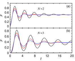
Figure 1: (Color online) Dynamics of the state transfer fidelity $F$ for the XX chain with identical interactions. The decoherence rate is given by $\gamma=0.1$ (black), $\gamma=0.2$ (red) and $\gamma=0.3$ (blue).

For infinite time $t$, the system evolves into a steady state with the transfer fidelity arrives at an asymptotic value $F^{\rm steady}(N)$, which can be obtained by combination of Eqs. (7), (19) and taking the infinite-time limit. After a tedious computation, we obtain

$$F^{\rm steady}(N)=\frac{3}{2(N+1)}.$$ (20)

Clearly, this steady state transfer fidelity is independent of the decoherence rate $\gamma$, and it solely decreases with the increase of the chain length $N$.

Next we consider time-dependence of the average fidelity for the XX spin chain with identical interactions and subject to intrinsic decoherence environments, with initial state prepared in the form of Eq. (9) in node A, i.e., $s=1$. From Fig. 2 one can see clearly that the average fidelity $\bar{F}$ also behaves as a damped oscillation as the time evolves. Here the relative small value for the case of $N=2$ is due to the fact that the phase of the state at node B is uncorrected, i.e., $\alpha$ is not a multiple of $2\pi$. When $t\rightarrow\infty$, the average fidelity also arrives at a steady state value, which is independent of the decoherence rate $\gamma$, and can be obtained analytically by taking the infinite-time limit of $\bar{F}$ from Eqs. (11), (14), and (16) as

$$\bar{F}^{\rm steady}(N)=\left\{\begin{aligned} &\frac{6N+17}{12N+12}\quad\rm if\quad\it N\in\rm odd,\\ &\frac{2N+3}{4N+4}\quad\quad\rm if\quad\it N\in\rm even.\end{aligned}\right.$$ (21)

Contrary to that of the initial state $|1\rangle$, this steady value does not decrease monotonously with the increase of the chain length $N$. However, as can be seen from Eq. (21), they decrease with the increase of the odd and even $N$, respectively, and approach to the asymptotic value 0.5 in the limit of $N\rightarrow\infty$.

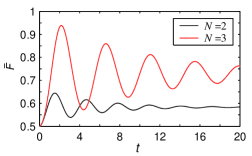
Figure 2: (Color online) Dynamics of the average fidelity $\bar{F}$ for the XX spin chain with identical interactions, where the decoherence rate is given by $\gamma=0.1$.

In the following we discuss quantum state transfer in intrinsic decoherence spin channels with fixed but different couplings between qubits. We consider the following modified Hamiltonian

$$\hat{H}=\sum_{n=1}^{N-1}\frac{J_{n,n+1}}{2}(\sigma_{n}^{x}\sigma_{n+1}^{x}+\sigma_{n}^{y}\sigma_{n+1}^{y}),$$ (22)

where $J_{n,n+1}=\lambda\sqrt{n(N-n)}$ is the modulated exchange coupling, and $\lambda$ is a scaling constant.

The above Hamiltonian is identical to the representation of the Hamiltonian $\hat{H}_{s}$ of a fictitious spin $S=(N-1)/2$ particle: $\hat{H}_{s}=\lambda S_{x}$, where $S_{x}$ is its angular momentum operator in $x$-direction and $\lambda$ is a scaling constant. For this Hamiltonian, its eigenvalues and corresponding eigenvectors can be obtained as [43]

$$E_{k}=(-N+2k-1)\lambda,\quad|\tilde{k}\rangle=\sum_{n=1}^{N}c_{k,n}|n\rangle.$$ (23)

where the coefficient $c_{k,n}$ is given by the following recursion relations

$$c_{1,1} = 1/2^{(N-1)/2},c_{k,1}=(-1)^{k+1}c_{1,k}$$

$$c_{k,n} = \frac{2E_{k}c_{k,n-1}-\sqrt{(n-2)(N-n+2)}c_{k,n-2}}{\sqrt{(n-1)(N-n+1)}}\quad(n\geqslant 2).$$

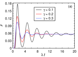
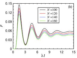
Figure 3: (Color online) Dynamics of the state transfer fidelity $F$ for the XX chain with modulated interactions. (a) chain length $N=100$ with different decoherence rate; (b) decoherence rate $\gamma=0.15$ with different chain length.

For this modulated chain, it has been shown that one can achieve perfect state transfer between the input node $n$ and the output node $N-n+1$ after a time $t_{0}=\pi/2\lambda$ and at intervals of $\pi/\lambda$ thereafter in the absence of decoherence environment [3,4]. When the intrinsic decoherence is present, however, this ideal spin channel will be destroyed, and it acts as an amplitude damping quantum channel as the rescaled time $\lambda t$ evolves. As can be seen from Fig. 3, the transfer fidelity $F$ oscillates around a steady state value, with the amplitude decreases gradually. This detrimental effects becomes more and more severe with the increase of the decoherence rate and the spin chain length, which is in consistent with the cases of the two- and three-site spin chains with identical interactions (In fact, they are two special cases of the interaction-modulated spin chain). This puts new constraints on these spin chains for long distance quantum state transfer. When $t\rightarrow\infty$, the transfer fidelity reaches a steady state value, which can be obtained from Eqs. (6), (7), (23), and (24) as

$$F^{\rm{steady}}(N)=\frac{1}{2^{2N-2}}\prod_{k=2}^{N}\left(4-\frac{2}{k-1}\right).$$ (25)

The steady state transfer fidelity of the interaction-modulated spin chain is still independent of the decoherence rate $\gamma$, and its magnitude is larger than its unmodulated counterparts [cf. Eqs. (20) and (25)], thought it still decreases with the increase of the chain length $N$.

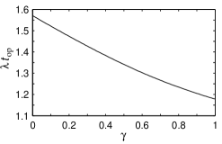
Figure 4: Dependence of $\lambda t_{\rm op}$ on decoherence rate $\gamma$. Note that the magnitudes of $\lambda t_{\rm op}$ is independent of the chain length $N$.

On the other hand, since the detrimental effects become severe as the rescaled time $\lambda t$ evolves, one may expect there exists an optimal time $\lambda t_{\rm op}$ at which the state transfer fidelity $F$ gets its maximum value. In Fig. 4 we show $\lambda t_{\rm op}$ versus the intrinsic decoherence rate $\gamma$, from which one can see that $\lambda t_{\rm op}$ is shifted to the left-hand side of $\lambda t_{0}=\pi/2\simeq 1.57$, and it decreases with the increase of $\gamma$. Our numerical results also revealed that the magnitudes of $\lambda t_{\rm op}$ is independent of the chain length $N$.

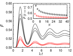
Figure 5: (Color online) Dynamics of the average fidelity $\bar{F}$ for the XX chain with modulated interactions, where the decoherence rate $\gamma=0.15$. The black lines from top to bottom correspond to chain length $N=101$, 151, and 201; whereas the red lines from top to bottom correspond to chain length $N=100$, 150, and 200. The inset shows the asymptotic value of the average fidelity for infinite time $t$ versus chain length $N$.

When considering the average fidelity, the numerical results calculated from Eqs. (11), (14), (23), and (24) show that it displays qualitatively the similar behaviors with that displayed in Fig. 3. The average fidelity decreases with increasing value of both odd and even $N$, respectively, and the chain with odd-number qubits seems to be more robust on creating high-fidelity state transfer in the presence of intrinsic decoherence (see Fig. 5). Moreover, as can be seen from the inset of Fig. 5, the average fidelity goes to a steady state value in the limit of $t\rightarrow\infty$, which has no relation with the decoherence rate $\gamma$. They decrease with the increase of both odd and even $N$, and approach the asymptotic value 0.5 in the limit of $N\rightarrow\infty$.

In the absence of intrinsic decoherence (i.e., $\gamma=0$), the above interaction-modulated spin chain can also be used to perfectly transfer an entangled state from one end of the chain to another [4]. When the decoherence is present, however, this ideal spin channel will be destroyed. For example, If one start with the Bell state $|\psi^{\pm}\rangle=(|01\rangle\pm|10\rangle)/\sqrt{2}$ on the first two qubits of the chain, the temporal evolution of the concurrence will behaves similarly as the state transfer fidelity, i.e., it acts as an amplitude damping channel. When the rescaled evolution time $\lambda t$ approaches infinite, from the formulae described in Section 2 one can obtain

$$C_{1,2}^{\rm{steady}}(N)=C_{N-1,N}^{\rm{steady}}(N)=\prod_{n=3}^{N}\frac{2n-5}{2n-4}.$$ (26)

In fact, one can show that for the initial state $|\psi\rangle=a|01\rangle\pm b|10\rangle$ $(|a|^{2}+|b|^{2}=1)$ prepared on the first two qubits, the following relation holds

$$C_{1,2}^{\rm{steady}}(N)=C_{N-1,N}^{\rm{steady}}(N)=C_{1,2}^{\rm{initial}}\prod_{n=3}^{N}\frac{2n-5}{2n-4},$$ (27)

where $C_{1,2}^{\rm{initial}}=2|ab|$ denotes the concurrence of the initial state of the first two qubits. This indicates that when the rescaled evolution time $\lambda t$ approaches infinite, the system goes to a steady mirror-symmetric state with two-qubit reduced density matrix $\rho_{nm}(t)=\rho_{N-n+1,N-m+1}(t)$, and the steady state value $C_{N-1,N}^{\rm{steady}}(N)=C_{1,2}^{\rm{steady}}(N)$ decreases as the chain length $N$ increases.

We now investigate entanglement distribution between two distant parties through the intrinsic decoherence spin channel. For this purpose, we assume the entangled state $|\psi\rangle=(|01\rangle+|10\rangle)/\sqrt{2}$ is initially prepared between a noninteracting qubit NI and the first qubit A on the chain, then after some time $t$, the entanglement will be established between NI and the target spin B. The overall Hamiltonian of the system can be written as $\hat{H}^{\prime}=I\otimes\hat{H}$, and with the same method used above, one can demonstrate that the concurrence $C_{\rm{NI,B}}(N,t)$ (Note that here $N$ denotes the length of the interacting-spin chain, and does not include the noninteracting qubit NI) also behaves as a damped oscillation, and when $t\rightarrow\infty$, we obtain

$$C_{\rm{NI,A}}^{\rm{steady}}(N) = C_{\rm{NI,B}}^{\rm{steady}}(N)$$ (28)

$$= \left\{\begin{aligned} &0\quad\rm\quad\quad\quad\quad\quad\quad if\quad\it N\in\rm odd,\\ &\prod_{n=3}^{(N+4)/2}\frac{2n-5}{2n-4}\quad\rm if\quad\it N\in\rm even.\end{aligned}\right.$$

This equation shows clearly that the XX chain with even-number qubits is more robust than its counterpart with odd-number qubits on distributing quantum entanglement. This is somewhat different from that of the average fidelity (see Fig. 5), where the chain with odd-number qubits is more efficient on creating high-fidelity state transfer in the presence of intrinsic decoherence.

4 Creating entanglement in decoherence environments

In this section, we see intrinsic decoherence effects on the creation of entanglement in various kinds of spin networks. For this purpose, we consider the multiarm structure $M(l_{1},l_{2},N_{A})$ of the XX Hamiltonian (22) with the addition of the exchange couplings between the hub site and its nearest-neighbor output sites satisfy the branching rule [10]. Here $l_{1}$ and $l_{2}$ denote the number of sites in the input and output arms, respectively, and $N_{A}$ is the number of output arms (see Fig. 6). It has been shown that in the absence of decoherence environment, this structure can be employed to create multi-qubit entangled $W$ state at the ends of the outgoing arms.

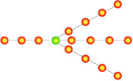
Figure 6: (Color online) Sketch of the multiarm structure of the spin network, where the green circle denotes the hub. The number of sites in the input and output arms are $l_{1}=3$, $l_{2}=4$, and the number of output arms is $N_{A}=3$.

The Hamiltonian in the subspace $\mathcal{H}_{1}$ spanned by the basis vectors $|n\rangle$ ($n=1,2,...,N$ ) is

$$\hat{H}=\sum_{(ij)}J_{ij}|i\rangle\langle j|+\rm H.c.,$$ (29)

where the summation runs over all pairs of neighboring spins. For the sake of simplicity, we first consider the Y-shaped structure $Y(l_{1},l_{2},2)$. The total number of sites now is $N=l_{1}+2l_{2}+1$. To examine temporal evolution of the concurrence of the prepared initial state, we make the following basis transformation for spins just in the same position of each arm

$$|n^{\pm}\rangle=\frac{1}{\sqrt{2}}(|n\rangle\pm|n^{\prime}\rangle),$$ (30)

where $n,n^{\prime}>l_{1}+1$. Then in the subspace spanned by $|n\rangle$ $(n\leqslant l_{1}+1)$ and $|n^{\pm}\rangle$ $(n>l_{1}+1)$, the Hamiltonian can be rewritten as

$$\hat{H} = \sum_{n<l_{1}+1}J_{n,n+1}|n\rangle\langle n+1|+$$ (31)

$$\sum_{n>l_{1}+1}\sum_{r=+,-}J_{n,n+1}|n^{r}\rangle\langle(n+1)^{r}|+$$

$$\sqrt{2}J_{l_{1}+1,l_{1}+2}|l_{1}+1\rangle\langle(l_{1}+2)^{+}|+\rm H.c.$$

Clearly, under the transformation (30) the Y-shaped structure is transformed into a linear chain consisting of the input arm, the hub and one output arm while the other output arm is decoupled (see Fig. 7), i.e., this structure is identical to the interaction-modulated one-dimensional XX chain with chain length $l=l_{1}+l_{2}+1$.

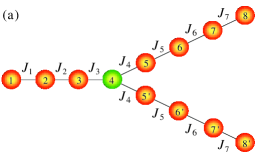
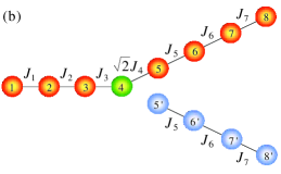
Figure 7: (Color online) (a) Sketch of the Y-shaped spin network. (b) Under the transformation (30) the Y-shaped structure is transformed into a linear chain consisting of the input arm and one output arm while the other output arm is decoupled.

For this spin network, if we prepare initial state $|1\rangle$ in the first node of the input arm, then after some time $t$, entanglement will be established between the end nodes of the output arms (for Fig.7, it corresponds to node 8 and $8^{\prime}$). From the formalism described in Section 2 one can obtain $C(l_{1},l_{2},\lambda,t)=F(l,\lambda,t)$. This implies that under the influence of intrinsic decoherence, the concurrence of the created entanglement between the end nodes of the output arms also behaves as a damped oscillation as the rescaled time $\lambda t$ evolves. For infinite rescaled evolution time $\lambda t\rightarrow\infty$, the concurrence goes to a steady state value $C^{\rm{steady}}(l_{1},l_{2})=2^{2-2l}\prod_{k=2}^{l}[4-2/(k-1)]$, which can be obtained directly from Eq. (25).

Similarly, for the multiarm structure $M(l_{1},l_{2},N_{A})$, using the same method, one can obtain that the concurrence measuring pairwise entanglement between arbitrary two qubits of the end nodes of the output arms is given by $C(l_{1},l_{2},N_{A},\lambda,t)=2F(l,\lambda,t)/N_{A}$ (when $N_{A}=2$, this equality reduces to that describing the Y-shaped structure), which observes the similar behaviors as the Y-shaped structure, i.e., it behaves as a damped oscillation as the rescaled time $\lambda t$ evolves, and when $\lambda t\rightarrow\infty$, it goes to a steady value $C^{\rm{steady}}(l_{1},l_{2},N_{A})=2^{3-2l}\prod_{k=2}^{l}[4-2/(k-1)]/N_{A}$.

5 Modified spin chains for high-fidelity state transfer

From the above arguments one can see that the interaction-modulated ideal spin channels for perfect state transfer are destroyed in the presence of intrinsic decoherence environments. Though there exists an optimal rescaled time at which one can get a relative high transfer fidelity, however, this transfer fidelity (including the average fidelity) decreases as the chain length $N$ increases, which puts great constrains for long distance communication in interacting-spin systems.

Here we demonstrate that a minor modification of the exchange interactions between the first and the last two nodes of the above structure can fulfill the requirements of long distance and near perfect state transfer (see Fig. 8a). To see this, we display our numerical results for chain length $N=11$ and $N=51$ in Fig. 9(a), from which one can see that for all decoherence rate $\gamma$, the maximum transfer fidelity $F_{max}$ approaches unity if $J_{0}$ is small enough (note that when $J_{0}=0$, $F\equiv 0$), which indicates that even in the presence of intrinsic decoherence environments, one can still achieve near perfect transfer of an excitation between the opposite ends of a XX chain by varying the strength of the exchange interactions between the first and the last two nodes of the modulated spin chain.

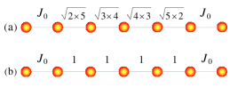
Figure 8: (Color online) Sketches of the two modified seven-site spin chains which may serve as spin channels for near perfect state transfer in the presence of intrinsic decoherence environments. Here we choose $N$ odd for it enables more efficient (i.e., high speed) state transfer than its counterpart with even $N$.

Another structure which may serve as near perfect spin channel for long distance transfer of an excitation in intrinsic decoherence environments is the XX quantum wire with the neighboring couplings except those between the first and the last two nodes are the same (see Fig. 8b). This chain can serve as spin channel for an almost perfect state transfer in the absence of decoherence environments [11]. When the intrinsic decoherence is present, from Fig. 9(b) one can see that a long distance transfer of an excitation whose fidelity can be arbitrarily close to unity is also possible for very small but nonzero $J_{0}$, even for large decoherence rate $\gamma$.

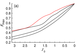
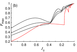
Figure 9: (Color online) Dependence of $F_{max}$ on $J_{0}$ for the two modified spin channels displayed in Fig. 8. In both figures the black lines from top to bottom correspond to chain length $N=11$ and decoherence rate $\gamma$=0.15, 0.30 and 0.45; whereas the red lines correspond to $N=51$ and $\gamma$=0.15. Note that when $J_{0}=0$, $F\equiv 0$.

To understand the above phenomenon, we sketch dynamics of $c_{\rm i}(t)$ in Fig. 10, where $c_{\rm i}(t)=\sqrt{\langle i|\rho_{i}(t)|i\rangle}$ denotes the amplitude of the coefficient for the state $|i\rangle$. From these two figures one can see that for very small but nonzero $J_{0}$, except the two end spins (here is node 1 and 11), the spins at the odd-number sites remain almost unexcited during the time evolution process (i.e., $c_{\rm i}(t)|_{\rm{i\in odd;i\neq 1,N}}\simeq 0$), as if the excitation is transferred only through the even-number nodes. In fact, a more detailed analysis show that if $J_{0}\rightarrow 0^{+}$ and $t\leqslant t_{\rm{op}}$, the mixedness of the system remain almost unchanged ($1-tr\rho^{2}\simeq 0$), i.e., the state here is very close to a pure state during the evolution process and thus can be described approximately by $|\psi(t)\rangle=c_{1}(t)|1\rangle+c_{N}(t)|N\rangle+\sum_{\rm{i\in even}}c_{i}(t)|i\rangle$, where $c_{1}(t)+c_{N}(t)\simeq 1$ (note that $c_{1}^{2}(t)+c_{N}^{2}(t)<1$ since $c_{\rm i}(t)|_{\rm{i\in even}}\neq 0$).

In order to better understand why the spins located at odd-number sites (the two end spins are exceptions) remain almost unexcited during the time evolution process for very small values of $J_{0}$, we graph the effects of decreasing $J_{0}$ on the eigenvector population $c_{k,1}^{2}=\{|\langle\hat{k}|1\rangle|^{2}\}_{E_{k}}$ for the two modified spin chains in Fig. 11, from which one can see that with decreasing values of $J_{0}$, the distribution of the eigenvectors becomes narrower and narrower. Particularly, in the limitation $J_{0}\rightarrow 0^{+}$, $\{|\langle\hat{k}|1\rangle|^{2}\}_{E_{k}}\neq 0$ only for the three central eigenvectors of the system, i.e., $c_{k,1}\neq 0$ only when $k_{1}=(N-1)/2$, $k_{2}=(N+1)/2$ and $k_{3}=(N+3)/2$. Moreover, for these three values of $k$, it can be shown that when $J_{0}\rightarrow 0^{+}$, $c_{k,n}\neq 0$ only when $n=1$, $N$ and $n\in\rm{even}$ for $k=k_{1}$, $k_{3}$, and $n=1$, $N$ for $k=k_{2}$. For example, when $N=11$, the eigenvectors of the Hamiltonian describing the first modified spin chain for the above three values of $k$ can be obtained as

$$\left\{\begin{aligned} &|\hat{k}_{1,3}\rangle=\frac{1}{2}(|1\rangle+|N\rangle)\mp\sqrt{\frac{5}{42}}(|2\rangle+|10\rangle)\mp\\ &\quad\quad\quad\sqrt{\frac{1}{12}}|6\rangle\pm\sqrt{\frac{15}{168}}(|4\rangle+|8\rangle),\\ &|\hat{k}_{2}\rangle=\sqrt{\frac{1}{2}}(|1\rangle-|N\rangle).\end{aligned}\right.$$ (32)

Similarly, for the second modified spin chain, its eigenvectors for the above three values of $k$ with arbitrary chain length $N$ ($N\in$ odd) can be obtained as

$$\left\{\begin{aligned} &|\hat{k}_{1,3}\rangle=\frac{1}{2}[|1\rangle+(-1)^{(N+1)/2}|N\rangle]\pm\\ &\quad\quad\quad\frac{1}{\sqrt{N-1}}\sum_{n\in\rm{even}}(-1)^{n/2}|n\rangle,\\ &|\hat{k}_{2}\rangle=\frac{1}{\sqrt{2}}[|1\rangle+(-1)^{(N-1)/2}|N\rangle].\end{aligned}\right.$$ (33)

On the other hand, for initial state $|1\rangle$ prepared in the input node A, the density matrix at arbitrary time $t$ can be obtained by choosing $\theta=\pi/2$, $\phi=0$ of Eqs. (10) and (11) as

$$\rho(t) = \sum_{n,m=1}^{N}\sum_{k,k^{\prime}=1}^{N}c_{k,1}c_{k^{\prime},1}c_{k,n}c_{k^{\prime},m}$$

$$\exp\left[-it(E_{k}-E_{k^{\prime}})-\frac{\gamma t}{2}(E_{k}-E_{k^{\prime}})^{2}\right]|n\rangle\langle m|.$$

Combination of Eq. (34) with the above arguments, one can conclude that the spins located at odd-number sites remain almost unexcited during the time evolution process, i.e., the excitation is transferred only through the even-number nodes for very small but nonzero values of $J_{0}$.

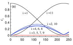
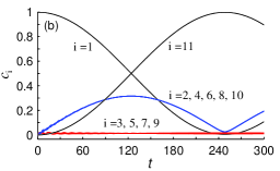
Figure 10: (Color online) Dynamics of $c_{\rm{i}}(t)$ for the two modified spin channels displayed in Fig. 8 with $J_{0}=0.02$, $\gamma=0.15$ and $N=11$. Here the curves for even-number $i$ (denoted by blue lines) are almost overlapped.

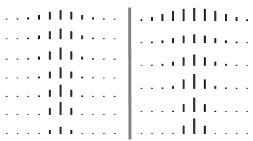
Figure 11: The eigenvector populations $\{|\langle\hat{k}|1\rangle|^{2}\}_{E_{k}}$ (denoted by the relative height of the vertical lines) for the system of 11 spins. The graphs from left to right in every plot correspond to the values of $k$ increases one by one (or equivalently, the eigenvalues increase one by one). The left seven panels correspond to the first modified spin chain with $J_{0}$=3, 2.5, 2, 1.5, 1, 0.5 and $J_{0}\rightarrow 0^{+}$ (from top to bottom), while the right six panels correspond to the second modified spin chain with $J_{0}$=1, 0.8, 0.6, 0.4, 0.2 and $J_{0}\rightarrow 0^{+}$ (from top to bottom).

In fact, from the formalism described in Section 2, one can see that the transfer fidelity of an excitation from one end of the chain to another is completely determined by

$$a_{NN} = \sum_{k,k^{\prime}=k_{1}}^{k_{3}}c_{k,1}c_{k^{\prime},1}c_{k,N}c_{k^{\prime},N}$$ (35)

$$\exp\left[-it(E_{k}-E_{k^{\prime}})-\frac{\gamma t}{2}(E_{k}-E_{k^{\prime}})^{2}\right],$$

where the coefficients of the eigenvectors for the three values of $k$ are given by

$$c_{k_{1},1} = c_{k_{3},1}=\frac{1}{2},\quad c_{k_{1},N}=c_{k_{3},N}=\frac{(-1)^{(N+1)/2}}{2},$$

$$c_{k_{2},1} = \frac{1}{\sqrt{2}},\quad c_{k_{2},N}=\frac{(-1)^{(N-1)/2}}{\sqrt{2}}.$$ (36)

On the other hand, the eigenvalues of the two modified spin chains correspond to the three eigenvectors $\{|\hat{k}_{1}\rangle,|\hat{k}_{2}\rangle,$ $|\hat{k}_{3}\rangle\}$ can be written as $\{-E_{0},0,E_{0}\}$ ($E_{0}$ can be obtained numerically), thus from the above two equations and the formalism described in Section 2, one can obtain the transfer fidelity of one excitation as

$$F = \frac{3}{8}+\frac{1}{8}\exp(-2\gamma E_{0}^{2}t)\cos(2E_{0}t)-$$ (37)

$$\frac{1}{2}\exp\left(\frac{-\gamma E_{0}^{2}t}{2}\right)\cos(E_{0}t)\quad(N\in\rm{odd}).$$

Since $E_{0}$ is very small in the limit of $J_{0}\rightarrow 0^{+}$, from Eq. (37) one can see that an almost perfect transfer of an excitation from one end of the chain to another occurs after time $t_{c}\sim\pi/E_{0}$. Moreover, we noted that $E_{0}$ decreases with the decrease of $J_{0}$, thus the critical time at which the transfer fidelity $F$ gets its maximum value increases with the decrease of $J_{0}$, and is independent of the decoherence rate $\gamma$. These conclusions can be corroborated by numerical results displayed in Fig. 10. For the system parameters adopted there (i.e., $N=11$, $J_{0}=0.02$), $E_{0}$ can be obtained numerically as $E_{01}\simeq 0.013801$ and $E_{02}\simeq 0.012648$, thus one has $t_{c1}\sim 227$ and $t_{c1}\sim 248$. Clearly, these results agree well with those displayed in Fig. 10.

A similar analysis shows that for the two modified spin chains with even-number qubits, the behavior of the transfer fidelity is determined only by the two central eigenvectors of the system in the limit of $J_{0}\rightarrow 0^{+}$, i.e., $c_{k,1}\neq 0$ only when $k_{1}=N/2$ and $k_{2}=N/2+1$. The eigenvectors of the Hamiltonian describing both the two modified spin chains for the above two values of $k$ can be obtained as

$$\left\{\begin{aligned} &|\hat{k}_{1}\rangle=\frac{1}{\sqrt{2}}[|1\rangle+(-1)^{N/2}|N\rangle],\\ &|\hat{k}_{2}\rangle=\frac{1}{\sqrt{2}}[|1\rangle-(-1)^{N/2}|N\rangle],\end{aligned}\right.$$ (38)

with the corresponding eigenvalues $-E_{0}$ and $E_{0}$. Combination of these with the formalism in Section 2, the transfer fidelity of one excitation can be obtained as

$$F=\frac{1}{2}-\frac{1}{2}\exp(-2\gamma E_{0}^{2}t)\cos(2E_{0}t)\quad(N\in\rm{even}).$$ (39)

From Eq. (38) one can see that in the limit of $J_{0}\rightarrow 0^{+}$, except the two spins located at the end nodes, all the other spins remain almost unexcited during the time evolution process, as if the excitation is transferred only between the two end nodes. Moreover, from Eq. (39) one can see that an almost perfect transfer of an excitation from one end of the chain to another occurs after time $t_{c}\sim\pi/2E_{0}$. However, our numerical results show that the values of $E_{0}$ for odd $N$ is much larger than that for even $N$ (e.g., for $J_{0}=0.001$, the values of $E_{0}$ for $N=11$ is about 2524 and 2804 times larger than that for $N=10$ and 12), thus the chain with odd $N$ enables a more efficient (i.e., high speed) state transfer than its counterpart with even $N$.

As a final discussion, it is worthwhile to investigate the efficiency of the above two modified spin channels, i.e., whether they can serve as near perfect spin channels for transfer of an arbitrary one-qubit state by varying the strength of $J_{0}$. For this purpose, we compute the average fidelity. From the above analysis one can obtain straightforwardly that in the limit of $J_{0}\rightarrow 0^{+}$, the average fidelity can be expressed as

$$\bar{F}=\frac{|b_{N}|\cos(\alpha)}{3}+\frac{a_{NN}}{6}+\frac{1}{2},$$ (40)

where the coefficients for odd and even $N$ are given by

$$a_{NN} = \frac{3}{8}+\frac{1}{8}\exp(-2\gamma E_{0}^{2}t)\cos(2E_{0}t)-$$

$$\frac{1}{2}\exp\left(\frac{-\gamma E_{0}^{2}t}{2}\right)\cos(E_{0}t),$$

$$b_{N} = \frac{(-1)^{(N-1)/2}}{2}\left[1-\exp\left(\frac{-\gamma E_{0}^{2}t}{2}\right)\cos(E_{0}t)\right],$$

and

$$a_{NN} = \frac{1}{2}-\frac{1}{2}\exp(-2\gamma E_{0}^{2}t)\cos(2E_{0}t),$$

$$b_{N} = (-1)^{N/2}i\exp\left(\frac{-\gamma E_{0}^{2}t}{2}\right)\sin(E_{0}t).$$ (42)

As pointed above, $E_{0}$ is an infinitesimal in the limit of $J_{0}\rightarrow 0^{+}$, thus from Eqs. (40) and (41) one can see obviously that for odd $N$, the average fidelity approaches unity after time $t_{c}\sim\pi/E_{0}$. For even $N$, however, due to the fact that $\alpha=\pi/2$ is not a multiple of $2\pi$, the average fidelity can only reach its maximum value $2/3$ (equals to the classical average fidelity) after time $t_{c}\sim\pi/2E_{0}$. This implies that for the above two modified spin channels with even $N$, one cannot achieve near perfect state transfer of an arbitrary one-qubit state simply by varying the strength of $J_{0}$. But if one can apply an external magnetic field $B$ along the $z$ axis of every spin (this does not change the eigenvectors of the system since $[\hat{H},\sigma_{\rm{tot}}^{z}]=0$), the phases of the received state at the destination node may be corrected. With this method, we performed numerous calculations and the numerical results revealed that the average fidelity can also approaches unity by choosing appropriate strength of the magnetic field (e.g., for $N=10$, $J_{0}=0.01$ and $B=\pm 0.0003$, the two modified spin channels give rise to $\bar{F}_{max}=0.9998$ and $\bar{F}_{max}=0.9996$, respectively).

6 Summary

To summarize, we have investigated quantum state transfer, generation and distribution of entanglement in the model of Milburn’s intrinsic decoherence environment. We focused on diverse interaction-modulated spin networks which may serve as perfect spin channels in the absence of decoherence. As one expected, the state transfer fidelity as well as the amount of the generated and distributed entanglement will be significantly lowered by the intrinsic decoherence environment, and this detrimental effects become severe as the decoherence rate $\gamma$ and the spin chain length $N$ increase. For infinite evolution time $t$, we show analytically that both the state transfer fidelity (including the average fidelity) and the concurrence of the generated and distributed entanglement approach steady state values, which are independent of the decoherence rate $\gamma$. This brings great constraints on these structures as spin channels for long distance and high-fidelity communication. Finally, as alternative schemes to diminish the detrimental effects, we presented two modified spin chains which may serve as spin channels for long distance and near perfect state transfer in the intrinsic decoherence environments. Our results revealed that in the limit of $J_{0}\rightarrow 0^{+}$, these two modified spin channels generate maximum fidelity 1 after certain time $t_{c}\sim\pi/E_{0}$ for spin chains with odd-number qubits. For spin chains with even-number qubits, however, one needs to apply an external magnetic field in order to achieve near perfect state transfer.

Acknowledgements

This work was supported by the National Natural Science Foundation of China under Grant No. 10547008, the Specialized Research Program of Education Bureau of Shaanxi Province under Grant No. 08JK434, and the Youth Foundation of Xi’an Institute of Posts and Telecommunications under Grant No. ZL2008-11.

References

- (1) S. Bose, Phys. Rev. Lett. 91, 207901 (2003)
- (2) T.J. Osborne, N. Linden, Phys. Rev. A 69, 052315 (2004)
- (3) M. Christandl, N. Datta, A. Ekert, A.J. Landahl, Phys. Rev. Lett. 92, 187902 (2004)
- (4) M. Christandl, N. Datta, T.C. Dorlas, A. Ekert, A. Kay, A.J. Landahl, Phys. Rev. A 71, 032312 (2005)
- (5) Y. Li, T. Shi, B. Chen, Z. Song, C.P. Sun, Phys. Rev. A 71, 022301 (2005)
- (6) T. Shi, Y. Li, Z. Song, C.P. Sun, Phys. Rev. A 71, 032309 (2005)
- (7) M.-H. Yung, S. Bose, Phys. Rev. A 71, 032310 (2005)
- (8) D. Burgarth, S. Bose, Phys. Rev. A 71, 052315 (2005)
- (9) D. Burgarth, S. Bose, New J. Phys. 7, 135 (2005)
- (10) I. D’Amico, B.W. Lovett, T.P. Spiller, Phys. Rev. A 76, 030302 (2007)
- (11) A. Wójcik, T. Łuczak, P. Kurzyński, A. Grudka, T. Gdala, M. Bednarska, Phys. Rev. A 72, 034303 (2005)
- (12) R.H. Crooks, D.V. Khveshchenko, Phys. Rev. A 77, 062305 (2008)
- (13) J.F. Zhang, G.L. Long, W. Zhang, Z.W. Deng, W.Z. Liu, Z.H. Lu, Phys. Rev. A 72, 012331 (2005)
- (14) V. Kostak, G.M. Nikolopoulos, I. Jex, Phys. Rev. A 75, 042319 (2007)
- (15) M.A. Jafarizadeh, R. Sufiani, Phys. Rev. A 77, 022315 (2008)
- (16) G. Gualdi, V. Kostak, I. Marzoli, P. Tombesi, Phys. Rev. A 78, 022325 (2008)
- (17) M. Paternostro, G.M. Palma, M.S. Kim, G. Falci, Phys. Rev. A 71, 042311 (2005)
- (18) A. Kay, Phys. Rev. A 73, 032306 (2006)
- (19) J.F. Zhang, X.H. Peng, D. Suter, Phys. Rev. A 73, 062325 (2006)
- (20) O. Romero-Isart, K. Eckert, A. Sanpera, Phys. Rev. A 75, 050303 (2007)
- (21) C. Di Franco, M. Paternostro, M.S. Kim, Phys. Rev. Lett. 101, 230502 (2008)
- (22) C. Di Franco, M. Paternostro, D.I. Tsomokos, S.F. Huelga, Phys. Rev. A 77, 062337 (2008)
- (23) M. Markiewicz, M. Wieśniak, Phys. Rev. A 79, 054304 (2009)
- (24) X.X. Yi, H.T. Cui, X.G. Wang, Phys. Lett. A 306, 285 (2003)
- (25) A.R.R. Carvalho, F. Mintert, A. Buchleitner, Phys. Rev. Lett. 93, 230501 (2004)
- (26) J. Wang, H. Batelaan, J. Podany, A.F. Starace, J. Phys. B 39, 4343 (2006)
- (27) A. Abliz, H.J. Gao, X.C. Xie, Y.S. Wu, W.M. Liu, Phys. Rev. A 74, 052105 (2006)
- (28) S.B. Li, J.B. Xu, Phys. Lett. A 311, 313 (2003)
- (29) S.B. Li, J.B. Xu, Phys. Lett. A 334, 109 (2005)
- (30) B. Shao, T.H. Zeng, J. Zou, Commun. Theor. Phys. 44, 255 (2005)
- (31) M. Hein, W. Dür, H.-J. Briegel, Phys. Rev. A 71, 032350 (2005)
- (32) J.M. Cai, Z.W. Zhou, G.C. Guo, Phys. Rev. A 74, 022328 (2006)
- (33) P.F. Yu, J.G. Cai, J.M. Liu, G.Y. Shen, Eur. Phys. J. D 44, 151 (2007)
- (34) Z. Sun, X.G. Wang, Y.B. Gao, C.P. Sun, Eur. Phys. J. D 46, 521 (2008)
- (35) A. Montakhab, A. Asadian, Phys. Rev. A 77, 062322 (2008)
- (36) Z.G. Li, S.M. Fei, Z.D. Wang, W.M. Liu, Phys. Rev. A 79, 024303 (2009)
- (37) G. J. Milburn, Phys. Rev. A 44, 5401 (1991)
- (38) S. Schneider, G.J. Milburn, Phys. Rev. A 57, 3748 (1998)
- (39) M. Abdel-Aty, Phys. Lett. A 372, 3719 (2008)
- (40) K. Kimm, H.-h. Kwon, Phys. Rev. A 65, 022311 (2002)
- (41) S. Hill, W.K. Wootters, Phys. Rev. Lett. 78, 5022 (1997)
- (42) W.K. Wootters, Phys. Rev. Lett. 80, 2245 (1998)
- (43) M.L. Hu, X.Q. Xi, Acta Phys. Sin. 57, 3319 (2008)