Study of the neoclassical radial electric field of the TJ-II flexible heliac

Abstract

Calculations of the monoenergetic radial diffusion coefficients are presented for several configurations of the TJ-II stellarator usually explored in operation. The neoclassical radial fluxes and the ambipolar electric field for the standard configuration are then studied for three different collisionality regimes, obtaining precise results in all cases.

1 Introduction

Radial electric fields are recognized to play a key role in the radial transport of stellarators. From the neoclassical transport point of view, they affect the particle orbits [helander2002collisional, wakatani1998stellarator]: for low-collisionality plasmas, they suppress the unfavorable $1/\nu$ regime [galeev1979theory] and allow for the formation of electron transport barriers, see Ref. [yokoyama2007cerc] and references therein. Additionally, radial electric fields and plasma rotation are tightly connected: it is considered that sheared $E\times B$ flows are likely to reduce the edge turbulence level thus facilitating access to High confinement (H) mode, see Refs. [burrell1997shearflow, wagner2007hmode] and references therein. A review on internal transport barriers and H mode in helical systems can be found in Ref. [wagner2006barriers]. Both effects have been measured at the heliac TJ-II [alejaldre1999first]: transitions to core electron root confinement have been observed in Electron Cyclotron Heated (ECH) plasmas [castejon2002cerc]. Transitions to H mode have been documented [sanchez2009transitions, estrada2009transitions] together with mean and low frequency oscillating sheared $E\times B$ flows in plasmas heated by Neutral Beam Injection (NBI).

Neoclassical transport theory allows to predict the radial electric field in helical devices by means of the ambipolarity condition. Examples of these calculations exist for devices such as W7-AS [kick1999w7as] and LHD [yokoyama2002lhd] among many others [yokoyama2007cerc, maassberg1993stellarators]. Previous neoclassical transport calculations of the ambipolar electric field at TJ-II include ECH plasmas [tribaldos2001nctj2, chmyga2002hibp, turkin2011predictive] and also medium-density NBI plasmas [zurro2006rotation]. In Refs. [chmyga2002hibp, zurro2006rotation], the calculations were compared with Heavy Ion Beam Probe (HIBP) and passive emission spectroscopy measurements: qualitative agreement was obtained. A number of additional HIBP measurements exist for ECH plasmas [krupnik2005hibp, melnikov2005hibp, milligen2011transitions], and more recently for NBI plasmas [melnikov2007hibp]. Near the edge, the electric field has been measured by means of reflectometry [estrada2006refle, estrada2009transitions] and, very recently, by studying mode rotation velocities [milligen2011islands].

Ref. [tribaldos2001nctj2] includes a comprehensive study of the transport coefficients and the flux balances for two ECH plasmas (although no multiple roots were found, see below), but an analogous work is missing for medium-density NBI plasmas, where only the ambipolar electric field has been shown. Furthermore, lithium wall coating of TJ-II has recently allowed [sanchez2009transitions] transitions to regimes of relatively high density in NBI plasmas, and these plasmas have not yet been described from the neoclassical transport point of view. Additionally, many of the effects reported above show a dependence on the magnetic configuration [estrada2004cerc, estrada2009transitions]. No qualitative changes are expected in the neoclassical radial transport of these configurations since the main Fourier components of the magnetic field strength do not change too much [solano1988tj-ii, tribaldos2001nctj2]. Still, the flexibility of TJ-II allows for exploring a large set of configurations (on a shot-to-shot basis [alejaldre1999confinement] or continuously [lopez2009cmode]) and a general study of the variation of the transport coefficients and the neoclassical balance may be of interest. More precise calculations for selected discharges are underway.

In this work, we aim to complete the previous neoclassical transport studies in view of the recent upgrades in TJ-II operation: we study a low-density ECH plasma and discuss, for the first time in detail from the neoclassical transport point of view, the issue of multiple roots at TJ-II. We also study a high-density NBI plasma and show for the first time the radial fluxes. Finally, we extend the calculations in these two plasmas to seven other configurations usually operated at TJ-II. The paper is organized as follows: the basic theory is reviewed in Section 2. The monoenergetic radial transport coefficient for the 100_44_64 magnetic configuration, the most usually operated at TJ-II, is briefly described in Section 3.1. Then, convolution and solution of the ambipolar equation yield the radial fluxes and the radial electric field for the two plasmas. A Monte-Carlo technique for error propagation allows us to account for the convergence problems of DKES [hirshman1986dkes] for the long-mean-free-path (lmfp), enhanced by the complexity of the magnetic configuration of TJ-II. This is done in Section 3.2. Finally we have explored part of the set of magnetic configurations of TJ-II with DKES calculations. In Section 3.3 we compare the main Fourier coefficients describing the equilibria, show how the monoenergetic radial transport coefficient depends on the configuration and finally discuss the implications on the radial particle balance. Section 4 is devoted to the conclusions.

2 Determination of the neoclassical radial fluxes

The radial electric field $E_{\mathrm{r}}$ may be obtained from the ambipolar condition of the neoclassical radial particle fluxes, which in a pure plasma composed of electrons and ions reads:

$$\Gamma_{\mathrm{e}}(E_{\mathrm{r}})=\Gamma_{\mathrm{i}}(E_{\mathrm{r}})\,.\\$$ (1)

The neoclassical fluxes are linear combinations of the density and temperature gradients and the radial electric field [helander2002collisional, wakatani1998stellarator]. For each species $\mathrm{b}$, the flux-surface-averaged radial particle flux $\Gamma_{\mathrm{b}}$ and radial energy flux $Q_{\mathrm{b}}$ are:

$$\frac{\Gamma_{\mathrm{b}}}{n} = -L_{11}^{\mathrm{b}}\left(\frac{1}{n}\frac{\mathrm{d}n}{\mathrm{d}r}-Z_{\mathrm{b}}e\frac{E_{\mathrm{r}}}{T_{\mathrm{b}}}-\frac{3}{2}\frac{1}{T_{\mathrm{b}}}\frac{\mathrm{d}T_{\mathrm{b}}}{\mathrm{d}r}\right)-L_{12}^{b}\frac{1}{T_{\mathrm{b}}}\frac{\mathrm{d}T_{\mathrm{b}}}{\mathrm{d}r}\,,$$ (2)

$$\frac{Q_{\mathrm{b}}}{nT_{\mathrm{b}}} = -L_{21}^{\mathrm{b}}\left(\frac{1}{n}\frac{\mathrm{d}n}{\mathrm{d}r}-Z_{\mathrm{b}}e\frac{E_{\mathrm{r}}}{T_{\mathrm{b}}}-\frac{3}{2}\frac{1}{T_{\mathrm{b}}}\frac{\mathrm{d}T_{\mathrm{b}}}{\mathrm{d}r}\right)-L_{22}^{b}\frac{1}{T_{\mathrm{b}}}\frac{\mathrm{d}T_{\mathrm{b}}}{\mathrm{d}r}\,.$$ (3)

Here $n$ is the density, and $T_{\mathrm{b}}$ and $Z_{\mathrm{b}}e$ are the temperature and the charge. We consider current free operation, $E_{\parallel}\!=\!0$. The thermal coefficients $L^{\mathrm{b}}_{\mathrm{j}\mathrm{k}}$ at each radial position can be calculated by convolution with a Maxwellian distribution of the monoenergetic radial diffusion coefficient:

$$L^{\mathrm{b}}_{\mathrm{j}\mathrm{k}}(r,n,T_{\mathrm{i}},T_{\mathrm{e}},E_{\mathrm{r}})\!=\!\frac{2}{\sqrt{\pi}}\int_{0}^{\infty}\mathrm{d}\,x^{2}\,e^{-x^{2}}x^{1+2(\delta_{\mathrm{j},2}+\delta_{\mathrm{k},2})}D_{11}(r,\nu^{*},\Omega)\,.$$ (4)

The integration variable, $x\!=\!v/v_{\mathrm{t}\mathrm{h}}^{\mathrm{b}}$, is the particle velocity normalized by the thermal velocity. The monoenergetic radial transport coefficient $D_{11}$, which we discuss in Section 3.1, depends on the collisionality $\nu^{*}\!=\!\nu R/v\iota$ and the electric field parameter $\Omega\!\equiv\!E_{\mathrm{r}}/(vB_{0})$. Here, $\nu$ is the collision frequency, $\iota$ is the rotational transform, $R$ the major radius and $B_{0}$ is the (0,0) Fourier harmonic of the magnetic field strength in Boozer coordinates.

From Eqs. (1), (2), (3) and (4), it is clear that the determination of the radial electric field in helical plasmas is a non-linear problem due to the $L_{\mathrm{j}\mathrm{k}}(E_{\mathrm{r}})$ dependence. This may lead to several solutions or roots of the ambipolar condition [mynick1983roots] when solving the ambipolar equation by means of root-finding algorithms. When this happens, we select among ion root $E_{\mathrm{r}}^{\mathrm{i}}$ and electron root $E_{\mathrm{r}}^{\mathrm{e}}$ according to a thermodynamic condition: minimization of the generalized heat production rate due to neoclassical transport, see e.g. [turkin2011predictive, maassberg1993root]. $I\!<\!0$ ($I\!>\!0$) means that the electron (ion) root is selected, where

$$I=\int_{E_{\mathrm{r}}^{\mathrm{i}}}^{E_{\mathrm{r}}^{\mathrm{e}}}(\Gamma_{\mathrm{i}}-\Gamma_{\mathrm{e}})\mathrm{d}E_{\mathrm{r}}\,.$$ (5)

Note that the transition region between roots has been imposed to have zero radial width. Another option would have been to solve a diffusion equation for $E_{\mathrm{r}}$, instead of Eq. (1).

For error estimate, we follow the Monte-Carlo method described in Ref. [velasco2011bootstrap]: we start with a database of the radial diffusion coefficient $D_{11}(r,\nu^{*},\Omega)$ with the corresponding error bars. For every value of $r$, $\nu^{*}$ and $\Omega$, we give a numerical value to $D_{11}$ in Eq. (4) by employing a Gaussian random number and then solve Eq. (1). By repeating this procedure a number of times, we obtain averages and standard deviations of $E_{\mathrm{r}}$ and the other relevant quantities.

It must be noted that the neoclassical ordering may be violated at TJ-II [tribaldos2005global, velasco2009finite] if the widths of the ion drift-orbits are large. This makes the diffusive picture fail, and a convective term corresponding to ripple-trapped particles should be added to $\Gamma_{\mathrm{i}}$ in Eq. (1), leading to a smaller electric field. The higher the collisionality, the lower the correction. The incompressibility of the $E\times B$ drift, one of the approximations in the calculation [beidler2007icnts], is valid for the NBI plasmas, where the electric field is small in absolute value, but it may fail when the electron root is realized and the electric field is close to resonance values. This may also lead to underestimate the ion flux, and thus to overestimate the positive radial electric field. Finally, although the monoenergetic calculations do not conserve momentum, momentum-correction is negligible for the radial transport of non-quasisymmetric stellarators [maassberg2009momentum, lore2010quasi].

3 Calculation and results

3.1 The magnetic configuration and the radial diffusion monoenergetic coefficient

TJ-II is a four-period ($N\!=\!4$) flexible heliac of medium size, with strong helical variation of the magnetic axis and magnetic surfaces with bean-shaped cross-section and small Shafranov shift. The so-called 100_44_64 configuration (the most often employed during TJ-II operation) has a major radius of $R\!=\!1.504\,$m, its minor radius is $a\!=\!0.192\,$m and its volume-averaged magnetic field is $0.957\,$T. We stick to the vacuum equilibrium calculated using VMEC [hirshman1986vmec], which has a flat iota profile, with $\iota(0)\!=\!-1.551$ and $\iota(a)\!=\!-1.650$.

The radial diffusion coefficient has been calculated with DKES, in an independent simulation for each radial position and value of $\nu^{*}$ and $\Omega$. The distribution function has been described with up to 150 Legendre polynomials and 2548 Fourier modes. For the description of each magnetic surface, the largest 50 Fourier modes have been employed.

Fig. 1 shows the normalized radial diffusion coefficient $D^{*}_{11}\!=\!D_{11}/D_{11}^{\mathrm{p}}$ calculated for several values of the collisionality and the normalized electric field, at $\rho\!=\!0.7$. The normalization $D_{11}^{\mathrm{p}}$ is the value of $D_{11}$ in the plateau regime for the equivalent axisymmetric tokamak, as in Ref. [beidler2011ICNTS].

The Pfirsch-Schlüter (PS), plateau and long-mean-free-path (lmfp) regimes [wakatani1998stellarator] are clearly visible in Fig. 1, with a qualitative dependence on $\nu^{*}$ and $\Omega$ equal to that of the classical stellarator. The same behaviour has been reported for similar configurations of TJ-II and other stellarators [tribaldos2001nctj2, beidler2011ICNTS]. This text-book dependence of $D^{*}_{11}$ with $\nu^{*}$ and $\Omega$ can be summarized as follows:

• $\nu$ regime for high collisionalities, with reduction of transport for large radial electric fields due to $E\times B$ poloidal precession [igitkhanov2006impurity].

• Independence from $\nu^{*}$ and $\Omega$ for intermediate collisionality.

• $1/\nu$ dependence for low collisionalities and $\Omega\!=\!0$, suppressed by the electric field, which leads to $\nu$ and $\sqrt{\nu}$ regimes [galeev1979theory].

The large error bars for collisionalities lower than $10^{-4}$ might lead to inaccurate results for low-density plasmas, due to the $1/\nu$ dependence of the coefficient. In this work, these error bars have been propagated to the final results following the method described in Ref. [velasco2011bootstrap]: as we will see in Section 3.2, the collisionality is usually high enough so that this procedure yields accurate results.

A database of $D^{*}_{11}$ has been built in the ($\rho$,$\nu^{*}$,$\Omega$)-space, with $\rho$ between 0.1 and 1, $\nu^{*}$ between $3\times 10^{-5}$ and $3\times 10^{2}$ and $\Omega$ between 0 and $1\times 10^{-1}$. The convolution of Eq. (4) requires interpolation and extrapolation in this three-dimensional database. The interpolation is done by means of 3-point Lagrange, with $\nu^{*}$, $\Omega$ and $D^{*}_{11}$ in logarithmic scale. Since $D^{*}_{11}$ is calculated at several tens of radial positions, interpolation in $\rho$ is not necessary (but note that Eq. (4) is local, so that radial interpolation would not be required at this step). We have made use of the asymptotic collisional and collisionless limits [beidler2011ICNTS] where possible. Neither the choice of interpolation algorithm nor the extrapolation procedure affect significantly the final results [spong2005flow]. Integration has been made by means of Gauss-Laguerre of order 64 (order 200 yields compatible results).

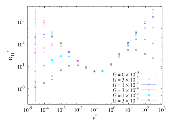
Figure 1: Monoenergetic radial diffusion coefficient at $\rho\!=\!0.7$ as a function of the collisionality for several values of the normalized electric field.

3.2 Radial balances

We calculate the ambipolar electric field for two regimes of TJ-II: a low-density ECH plasma (Figs. 2, 3, 4, 5 and 6) a high-density NBI plasma (Figs. 7, 8, 9 and 10). Since the walls are coated with lithium [tabares2008lithium], TJ-II plasmas have low impurity content, and the effective charge may be taken to be $Z_{\mathrm{eff}}\!=\!1\,$ everywhere.

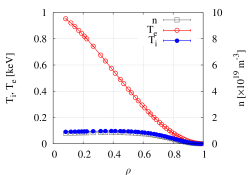
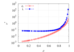
Figure 2: Plasma profiles for the low-density plasma: density and temperatures (left); collisionalities (right).

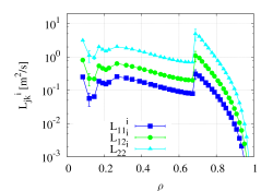
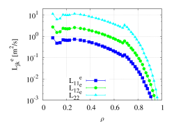
Figure 3: Thermal transport coefficients for the low-density plasma.

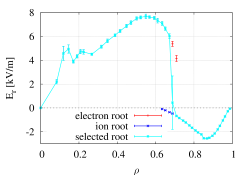
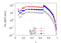
Figure 4: Radial balance for the low-density plasma: ambipolar radial electric field (left); ambipolar particle and energy fluxes (right).

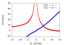
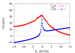
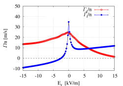
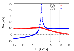
Figure 5: Radial particle fluxes as a function of the radial electric field at 4 radial positions of the ECH plasma: $\rho\!=\!0.22$ (top left), $\rho\!=\!0.61$ (top right), $\rho\!=\!0.65$ (bottom left) and $\rho\!=\!0.74$ (bottom right).

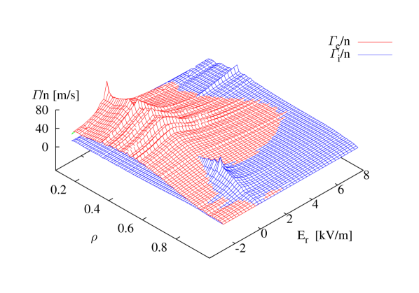
Figure 6: Radial profile of the solution of the ambipolarity equation for the ECH plasma.

First of all, the two plasmas show some common features: near the edge, both the temperatures and densities drop to zero in a way that the collisionality rises some orders of magnitude. As a result of this, the thermal coefficients will be very small and the neoclassical transport will be negligible: in this region, transport will be completely anomalous. Therefore, the calculated $E_{\mathrm{r}}$ may be relevant only if the dominant turbulence is electrostatic, and hence automatically ambipolar; the neoclassical radial fluxes are shown for the sake of completeness.

For electrons, one has almost everywhere $L^{\mathrm{e}}_{22}\!\gg\!L^{\mathrm{e}}_{21}\!\gg\!L^{\mathrm{e}}_{11}\,$, so the temperature gradient acts usually as the main drive for both the radial particle and energy flux. For ions, the three coefficients $L^{\mathrm{i}}_{\mathrm{j}\mathrm{k}}$ are somewhat closer, and the ion temperature is rather flat, so also the density gradient and the radial electric field are responsible for the radial fluxes.

The low-density plasma has a hollow density profile and a peaked electron temperature profile, with a central value around 1 keV, see Fig. 2. In these conditions, the electrons are in the lmfp regime, except near the edge, where the temperature drops. The ion temperature is lower, about 100 eV, and therefore the ions are in the plateau regime.

The thermal transport coefficients are larger for the electrons for $\rho\!<0.6$, see Fig. 3, and so is the temperature gradient. This yields a positive ambipolar radial electric field in Fig. 4. Fig. 5 shows the solution of the ambipolar equation at $\rho\!=\!0.22$ (top left) and $\rho\!=\!0.61$ (top right). At both positions, the radial electron flux, which is larger, is reduced by a non-zero electric field via the dependence $L^{\mathrm{e}}_{\mathrm{j}\mathrm{k}}(E_{\mathrm{r}})$. The ion radial flux is driven by the convective term $E_{\mathrm{r}}/T_{\mathrm{i}}$ (although at $\rho\!=\!0.61$, the effect of a radial electric field reducing the orbit width is clearly visible). At $\rho\!=\!0.22$, the poloidal resonance may be playing a role in $\Gamma_{\mathrm{i}}$ for $E_{\mathrm{r}}\sim 1\,kV/m$: the diffusion coefficient has a peak for the value of $E_{\mathrm{r}}$ such that the poloidal $E\times B$ drift and the poloidal parallel velocity cancel out, and then decreases. At outer positions, the electron collisionality is higher and the density and ion temperature gradients rise. In these conditions, the ion particle flux is larger than the electron flux for $\rho\!>\!0.61$. Around $\rho\!=\!0.65$ (bottom left of Fig. 5), two stable solutions for the ambipolar condition appear: as in inner positions, a positive electric field (electron root) which drives convectively the ions. But also a negative electric field (ion root) is able to bring ion transport to the electron level, via reduction of the radial excursions of trapped ions. At these conditions, electrons are the rate-controlling species (i.e., the ion radial flux is reduced to the electron level), and the particle flux is driven by the density and electron temperature gradients. Finally, closer to the edge, the electron transport drops, and only a negative electric field is able to restore ambipolarity. Bottom right of Fig. 5 shows this happening at $\rho\!=\!0.74$. The radial dependence of the ambipolar equation has been summarized in Fig. 6, where we show the radial particle fluxes as a function of $\rho$ and $E_{\mathrm{r}}$. The intersections of $\Gamma_{\mathrm{i}}(\rho,E_{\mathrm{r}})$ and $\Gamma_{\mathrm{e}}(\rho,E_{\mathrm{r}})$ give the profile of the radial electric field $E_{\mathrm{r}}(\rho)$.

This general behaviour is consistent with that obtained in calculations for similar magnetic configurations of TJ-II [tribaldos2001nctj2, turkin2011predictive] and to the experimental data from HIBP [chmyga2002hibp, melnikov2007hibp].

For a wide range of radial positions, $0.3\!<\!\rho\!<0.7$, the radial fluxes are very slowly decreasing (almost constant) functions of $\rho$. This happens because the ions, which are the rate controlling species, are driven by a radial electric field with low shear, $E_{\mathrm{r}}\sim\mathrm{d}T_{\mathrm{e}}/\mathrm{d}r$. A jump to higher fluxes may be observed for $\rho\!>\!0.7$ in Fig. 4, and thus a minimum of the radial fluxes at $\rho\!=\!0.7$, the point of maximum density and temperature gradients. The jump can also be seen in the thermal coefficients, see Fig. 3: it corresponds to the change of electron to ion root and it reflects the difference in the drift-orbit size for the two different absolute values of the radial electric field. The jump is thus larger for the ions, which is consistent with the data shown in Fig. 5 (bottom left). If $E_{\mathrm{r}}$ were obtained by solving a diffusion equation, the transition from electron to ion root would be smoother. Yet, the results of the calculations in Ref. [turkin2011predictive] suggest that the minima might remain, both in the particle flux and in the energy flux; the formation a particle transport barrier at $\rho\!=\!0.7$ has been observed in low-density transitions in ECH plasmas of TJ-II (see Ref. [milligen2011transitions] and references therein) but no simultaneous accumulation of energy has been detected.

During this low-density transition, a double poloidal-velocity shear layer has been measured near the edge [estrada2009transitions, milligen2011islands]. Although the formation of this layer is caused by anomalous transport, once the profiles are set the static electric field may be discussed in terms of neoclassical fluxes: the electron temperature (and thus the thermal transport coefficients) drops much faster than the ion temperature in the range $0.7\!<\!\rho\!<\!0.9$, and this requires a negative shear to maintain ambipolarity; the opposite happens for $\rho\!>\!0.9$, hence the positive shear in our calculation.

For NBI plasmas, the electron temperature is flatter and lower, since the plasma has reached the ECH-cutoff density. The ion temperature is still flat, and slightly higher due to the NBI heating. The lithium wall coating has allowed [sanchez2009transitions] transitions from plasmas of medium density ($\langle n\rangle\sim 2\times 10^{19}m^{-3}$) to plasmas of relatively high density ($\langle n\rangle\sim 5\times 10^{19}m^{-3}$). The studied plasmas are shown in Fig. 7: both the ions and the electrons are in the plateau regime, the ions being slightly more collisional. In these conditions, the thermal transport coefficients shown in Fig. 8 are larger for the ions, whose drift-orbit size is much larger. Since the electron temperature is rather flat except near $\rho\!=\!0.7$, the plasma is in the ion root everywhere, see Fig. 9. The solution of the ambipolar equation for these plasmas is shown in Fig. 10. The situation is similar to that of the ECH plasma near the edge: the radial ion flux, being larger, is reduced via $L^{\mathrm{i}}_{12}(E_{\mathrm{r}})$ to the electron level, which is in turn determined by the density and electron temperature gradients. The radial fluxes are maximum where the density and ion temperature gradients are larger.

The ambipolar $E_{\mathrm{r}}$ for the is qualitatively similar to that obtained for a similar magnetic configurations (and lower density) in Ref. [zurro2006rotation] and to HIBP measurements [melnikov2007hibp].

At TJ-II, the ion temperature is usually measured by a charge-exchange neutral particle analyzer [fontdecaba2004cxnpa] and the profiles, obtained on a shot-to-shot basis, are not always compatible with the ones deduced from spectroscopy measurements [zurro2006rotation]. It is therefore meaningful to allow for variations in the ion temperature profile in the neoclassical transport calculations. If $T_{\mathrm{i}}$ were slightly higher and more peaked than the $T_{\mathrm{i}}$ employed so far, no qualitative effects would be expected in ECH plasmas, since $E_{\mathrm{r}}$ is determined by the electron temperature. The ambipolar flux, being the ions the rate-controlling species, would probably be slightly larger. For the NBI plasmas, a more negative electric field is expected, maybe slightly peaked near the core region, with no major changes in the ambipolar flux.

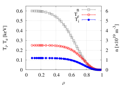
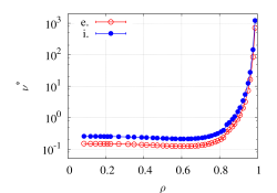
Figure 7: Plasma profiles for the high-density plasma: density and temperatures (left); collisionalities (right).

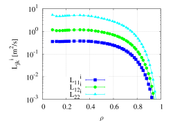
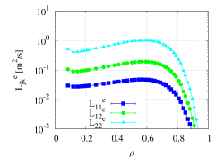
Figure 8: Thermal transport coefficients for the high-density plasma.

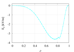
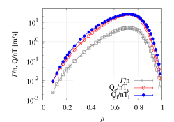
Figure 9: Radial balance for the high-density plasma: ambipolar radial electric field (left); ambipolar particle and energy fluxes (right).

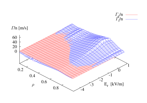
Figure 10: Radial profile of the solution of the ambipolarity equation for the NBI plasma.

Configuration name	$\langle B(T)\rangle_{vol}$	V($m^{3}$)	$\iota(0)$	$\iota(a)$
100_32_60	1.087	0.934	-1.423	-1.517
100_38_62	0.971	1.031	-1.492	-1.593
100_40_63	0.960	1.043	-1.510	-1.609
100_42_63	0.931	1.079	-1.534	-1.630
100_44_64	0.962	1.098	-1.551	-1.650
100_46_65	0.903	1.092	-1.575	-1.676
100_50_65	0.962	1.082	-1.614	-1.704
100_55_67	0.964	1.073	-1.659	-1.739

Table 1: Main parameters of the configuration scan.

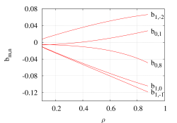
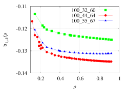
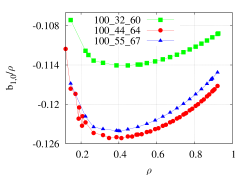
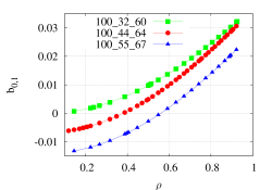
Figure 11: Main Fourier components of the 100_44_64 configuration (top left); helical curvature (top right), toroidal curvature (bottom left) and toroidal mirror (bottom right) for the configurations 100_32_60, 100_44_64, 100_55_67.

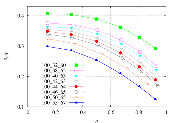
Figure 12: Profile of the effective curvature for all the configurations of the study.

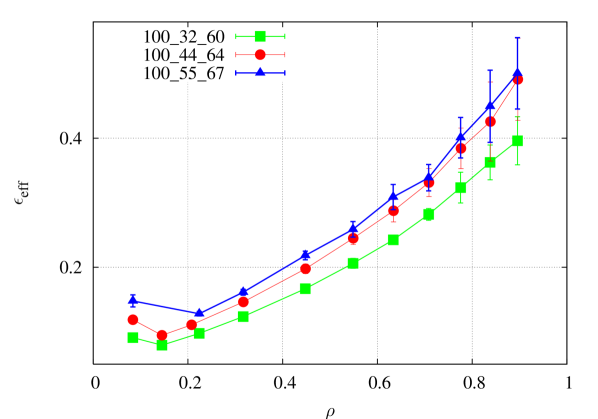
Figure 13: Profile of the effective ripple for the configurations 100_32_60, 100_44_64, 100_55_67.

3.3 Configuration dependence of the radial fluxes

Finally, we make a scan in a relevant part the configuration space of TJ-II. We study eight magnetic configurations usually explored in regular operation of TJ-II. Their main global parameters are shown in Table 1. The rotational transform at the magnetic axis varies about a 20% during the scan (and so does at the edge, since the profile shape is kept unchanged). Since the volume is approximately constant as well and the main Fourier terms in the description of the magnetic field do not change too much, no large differences in the neoclassical radial transport are expected [solano1988tj-ii]. Indeed the qualitative behaviour is identical to that of Fig. 1. We thus make a discussion on the radial profile of several quantities that parametrize the dependence on $\nu^{*}$ of the monoenergetic coefficient for the 100_44_64 configuration and the others.

The two main contributions to the radial diffusion should come from the helical ($b_{1,-1}$) and toroidal ($b_{1,0}$) curvatures and the toroidal mirror ($b_{0,1}$) in the Fourier decomposition of $B$ given by:

$$B(\rho,\phi,\theta)/B_{0}(\rho)=\sum_{n=-\infty}^{\infty}\sum_{m=0}^{\infty}b_{m,n}(\rho)cos(m\theta-Nn\phi)\,,$$ (6)

where $\phi$ and $\theta$ are Boozer coordinates. They are shown in Fig. 11 for three of the configurations of the scan: 100_44_64, 100_32_60, 100_55_67 (the center and the extremes of the scan).

In the PS regime, for $\Omega\!=\!0\,$, we have $D^{*}_{11}\!\propto\!\kappa^{-1}\nu^{*}\,$ [igitkhanov2006impurity]. Here, $\kappa\propto(b_{1,0})^{-2}$ is called toroidal curvature. The small correction for large $\Omega$ depends weakly on $\iota$ and $R$.

According to Fig. 11, we can expect the collisional transport of these configurations to be quite similar. Nevertheless, modulation of the toroidal mirror term $b_{0,1}$ allows for optimization of radial transport in elongated configurations (see e.g. Ref [beidler2011ICNTS]). In Ref. [aizawa2000curvature], an effective toroidal curvature was defined, including $b_{1,0}$ and $b_{0,1}$, in order to account for this effect. The latter Fourier term has a large relative (although not absolute) variation in this configuration scan [velasco2011bootstrap]. From the slope of $D^{*}_{11}$ for high $\nu^{*}$ in Fig. 1 one can calculate an effective curvature $\kappa_{\mathrm{eff}}$ defined by:

$$D^{*}_{11}(\nu^{*}\to\infty,\Omega=0)=\frac{32}{3\pi}\frac{\nu^{*}}{\kappa_{\mathrm{eff}}}\,.$$ (7)

Therefore, from the slope of $D^{*}_{11}$ for high $\nu^{*}$ in Fig. 1 one can extract the local value of $\kappa_{\mathrm{eff}}$. The profile of this quantity is shown in Fig. 12. There is a $\iota^{-2}$ scaling (see Table 1) at every radial position in our set of configurations, so we focus, from now on, on the extremes of the scan. Since $D_{11}^{\mathrm{p}}\!\propto\!(\iota B_{0}^{2})^{-1}$ and $\nu^{*}\!\propto\!\iota^{-1},$ the contribution of the PS regime to the thermal transport coefficient is $L_{11}\!\propto\!(\kappa_{\mathrm{eff}}\iota^{2}B_{0}^{2})^{-1}$. These results altogether yield a neoclassical transport in the configuration 100_32_60 reduced with respect to the others (100_44_64 and 100_55_65) via the trivial scaling $L_{11}\!\propto\!B_{0}^{-2}\,$.

The results are different in the lmfp regime. In the limit case of classical stellarator (i.e., if only $b_{1,0}$ and $b_{1,-1}$ are non-zero in Eq. (6)), we have $D^{*}_{11}\!\propto\!(b_{1,-1})^{3/2}/\nu^{*}\,$ for $\Omega\!=\!0$ [galeev1979theory]. If more Fourier terms are non-zero, particle-trapping in local minima of the magnetic field leads to enhanced radial transport. However, one can still describe the radial diffusion in the lmfp regime in terms of an effective helical ripple $\varepsilon_{\mathrm{eff}}\,$[dommaschk1984ripple, beidler1994ripple, beidler2011ICNTS]. This quantity is defined by:

$$D^{*}_{11}(\nu^{*}\to 0,\Omega=0)=\left(\frac{4}{3\pi}\right)^{2}\frac{(2\varepsilon_{\mathrm{eff}})^{3/2}}{\nu^{*}}\,,$$ (8)

obtained from data such as Fig. 1. It contains information of the helical ripple $b_{1,-1}$, as well as of all the other terms in Eq. (6). In Fig. 13 we show the radial profile of the effective ripple for three of the configurations: 100_32_60, 100_44_64, 100_55_67. The configuration 100_32_60 has a smaller effective ripple, while those of the 100_44_64 and 100_55_67 configurations are quite close. Since, for the lmfp regime, one has $L_{11}\!\propto\!\varepsilon_{\mathrm{eff}}^{3/2}B_{0}^{-2}\,$, the latter configurations will have similar radial neoclassical transport. Configuration 100_32_60 will have considerably smaller transport, and the reduction will be larger than the $L_{11}\!\propto\!B_{0}^{-2}\,$ of the PS regime.

These results altogether lead to a reduced radial neoclassical transport for the 100_32_60 configuration with respect to the 100_44_64, 100_55_67 configurations. The reduction is larger for the electrons (which have a larger contribution of the lmfp regime) than for the ions (which are more collisional). Consequently, this will affect, via the ambipolar condition, the neoclassical radial electric field, which will be smaller. This is consistent with impurity poloidal rotation measurements for ECH plasmas in Ref. [zurro2006rotation]. The results are shown in Fig. 14 for the profiles of the ECH plasma, see Fig. 2: the differences in $E_{\mathrm{r}}$ are larger for $\rho\!<\!0.7$, where the collisionality is lower. The radial particle fluxes are mainly reduced for $\rho\!>\!0.7$, where the ion-root is realized and thus the electrons are the rate-controlling species. The results for the NBI plasmas, shown in Fig. 15, are similar to that of the ECH plasma for $\rho\!>\!0.7$: a small reduction of the electric field (which now becomes more negative) together with a reduction of the ambipolar particle flux.

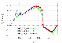
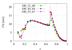
Figure 14: Ambipolar radial electric field (left) and radial particle fluxes (right) for configurations 100_32_60, 100_44_64, 100_55_67 and the profiles of Fig. 2.

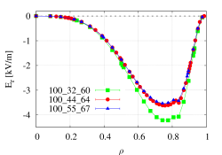
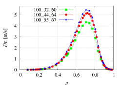
Figure 15: Ambipolar radial electric field (left) and radial particle fluxes (right) for configurations 100_32_60, 100_44_64, 100_55_67 and the profiles of Fig. 7.

4 Conclusions

We have presented calculations of the radial diffusion monoenergetic transport coefficient for several configurations of TJ-II. By convolution of these coefficients, we have calculated the ambipolar radial electric field and the fluxes for two different plasmas corresponding to the 100_44_64 configuration. The convolution included data with large error bars due to the poor convergence of DKES in the lmfp regime, but a Monte Carlo method for error propagation has allowed us to show that the results are accurate even for the ECH plasma.

The results for the ECH plasma are similar to the ones obtained in previous works. No such calculations exist for high-density NBI plasmas, but the some of the results shown here stay in qualitative agreement with the experiment. Future work includes comparison with HIBP and CXRS measurements for this kind of discharges.

Small quantitative and no qualitative differences have been found between configurations, since the Fourier spectra are very similar. The results predict that configurations with reduced $\iota$ lead, for the same plasma profiles, to slightly smaller radial electric field and to slightly improved particle confinement.

The results shown here extend the knowledge of neoclassical transport and radial electric field to regimes and configurations not explored previously at TJ-II.

5 Acknowledgments

The authors are grateful to D. Spong and S.P. Hirshman for the DKES and VMEC codes. Previous discussions with H. Maaßberg, C.D. Beidler and A. López-Fraguas, were very useful. Conversations with B Ph. Van Milligen, B. Zurro and I. Calvo improved the quality of the manuscript. This work has been partially funded by the Spanish Ministerio de Ciencia e Innovación, Spain, under Project ENE2008-06082/FTN.

References