Probing Substellar Companions of AGB Stars through Spirals and Arcs

Abstract

Recent observations of strikingly well-defined spirals in the circumstellar envelopes of asymptotic giant branch (AGB) stars point to the existence of binary companions in these objects. In the case of planet or brown dwarf mass companions, we investigate the observational properties of the spiral-onion shell wakes due to the gravitational interaction of these companions with the outflowing circumstellar matter. Three dimensional hydrodynamical simulations at high resolution show that the substellar mass objects produce detectable signatures, corresponding to density contrasts (10–200 %) and arm separations (10–400 AU) at 100 AU distance, for the wake induced by a Jupiter to brown dwarf mass object orbiting a solar mass AGB star. In particular, the arm pattern propagates in the radial direction with a speed depending on the local wind speed and sound speed, implying possible variations in the arm separation in the wind acceleration region and/or in a slow wind with significant temperature variation. The pattern propagation speeds of the inner and outer boundaries differ by twice the sound speed, leading to the overlap of high density boundaries in slow winds and producing a subpattern of the spiral arm feature. Vertically, the wake forms concentric arcs with angular sizes anticorrelated to the wind Mach number. We provide an empirical formula for the peak density enhancement as a function of the mass, orbital distance, and velocity of the object as well as the wind and local sound speed. In typical condition of AGB envelopes, the arm-interarm density contrast can be greater than 30 % of the background density within a distance of $\sim 10\,(M_{p}/M_{J})$ AU for the object mass $M_{p}$ in units of Jupiter mass $M_{J}$. These results suggest that such features may probe unseen substellar mass objects embedded in the winds of AGB stars and may be useful in planning future high sensitivity/resolution observations with ALMA.

1 INTRODUCTION

In high density environments, substellar companions leave their orbital imprints through the gravitational interaction with the surrounding circumstellar medium. An example is the observation of molecular spiral arms in the protoplanetary disk of AB Aurigae (Fukagawa et al., 2004), which is considered as evidence of a giant planet within the disk (Lin et al., 2006). It is now well established that a spiral wave sets up in the differentially rotating system (e.g., Goldreich & Tremaine, 1979; Masset, 2008, and references therein) during the formation and growth of a planet. This protoplanetary phase lasts for a few million years and is followed by a main sequence phase, in which the circumstellar disk dissipates and the planet-disk interaction ceases.

Planets or brown dwarfs orbiting low and intermediate mass stars ($M_{\ast}\leq 6-8$ $M_{\odot}$) may have another opportunity to interact with their immediate surroundings before the stars terminate their evolution as white dwarf remnants. Stars that have evolved off the main sequence, especially on the asymptotic giant branch (AGB), expel a large fraction of their mass at rates $\sim 10^{-7}-10^{-4}$ $M_{\odot}$ yr^-1, forming extensive ($10^{16}-10^{18}$ cm) cool ($10^{2}-10^{3}$ K) low velocity ($3-30$ km s^-1) outflowing envelopes (Habing & Olofsson, 2003; Fong et al., 2006, and references therein). Such intense mass loss rates imply an envelope density of $10^{-19}-10^{-16}$ $g$ cm^-3 at 100 AU distance from the stellar center, which is slightly lower than the typical density of protoplanetary disks (Hayashi, 1981; Aikawa & Herbst, 1999). Similar to the protoplanetary case, substellar mass objects that are embedded in the dense circumstellar envelopes of evolved giant stars will interact with the environment, playing a role in shaping the wind structure and also affecting the orbital evolution of the system.

Recently, the circumstellar envelopes of a few AGB stars have been found to possess spiral morphologies (e.g., Mauron & Huggins, 2006 for AFGL 3068; Dinh-V.-Trung & Lim, 2009 for CIT 6). Such structures cannot be explained by the spherically symmetric wind models for isolated stars with either continued (e.g., Parker, 1958; Gilman, 1972) or pulsating (e.g., Wood, 1979; Willson & Hill, 1979; Winters et al., 2000; Simis et al., 2001) mass ejection (for a review, see Lafon & Berruyer, 1991), although the pulsation models are able to explain the concentric shells and arcs of dust detected in a number of post-AGB or proto-planetary phases (e.g., Sahai et al., 1998; Mauron & Huggins, 1999; Kwok et al., 2001; Hrivnak et al., 2001). However, direct comparison with the detailed observational aspects remains as they likely involve the nonlinear process of dust formation in the envelopes. On the other hand, the spirals and greatly distended shells/arcs are more naturally produced by dynamical effects arising from a binary interaction in the expanding wind of the mass losing AGB star (Soker, 1994; Mastrodemos & Morris, 1999; He, 2007; Edgar et al., 2008). The binary-induced spiral model is supported by the detection of two point sources within the amazingly well-defined spiral envelope of AFGL 3068 (Morris et al., 2006).

Interestingly, albeit initiated from a different viewpoint, a very similar spiral-onion shell structure in three dimensional space was described by Kim & Kim (2007). This study may help facilitate an understanding of asymmetric morphologies in circumstellar envelopes for cases of companions with low masses, which are not sufficiently massive to displace the parent star due to orbital motion. Their linear perturbation analysis for gravitationally induced density wakes of circularly orbiting objects was motivated by Ostriker’s (1999) purely analytical formalism of the density wakes for linear orbit objects. Follow up studies were carried out for binaries (Kim et al., 2008), for heavy objects showing nonlinear aspects (Kim & Kim, 2009; Kim, 2010), and for objects in accelerated motion (Namouni, 2010). Kim & Kim (2009) noticed that the local features of the nonlinear density wake are conceptually the same as those of a Bondi-Hoyle-Lyttleton accretion column (see Edgar, 2004, and references therein), and are insensitive to the surface condition of the object.

We note that the above theoretical works are based on an initially static uniform medium, which differs from the expanding AGB envelopes. However, their results deserve to be examined in the extreme limit of a slow wind. The focus of these works was on the orbital evolution of the perturbing object due to dynamical friction, leaving the details of the wake itself in abeyance. In a separate paper (Kim, 2011, hereafter K11) the properties of the wake induced by a circularly orbiting object at distance $r_{p}$ with the orbital Mach number $\mathcal{M}_{p}$ ($>$1) in a static uniform background was investigated. Here, we compare the results for the outflowing envelopes to the case of a static background. The resulting wake in the latter is characterized by a single-armed Archimedes spiral in the orbital plane satisfying $r/r_{p}=\varphi\mathcal{M}_{p}^{-1}+1$, where $\varphi$ is the angular distance along the spiral pattern, and by arcs in meridional planes having the angular size of $2\tan^{-1}(\mathcal{M}_{p}^{2}-1)^{1/2}$. Its density contrast is determined by

$$\alpha_{1}=\frac{r_{B}}{|r-r_{p}|}\frac{1}{(\mathcal{M}_{p}^{2}-1)^{1/2}},$$ (1)

and the background density modification due to memory effect, where $r_{B}$ is the Bondi accretion radius of the perturbing object. In this paper, we investigate the effects of an outflowing background on the wake features both analytically and numerically in order to provide an interpretative framework of future observations for indirectly probing substellar mass objects in AGB envelopes. In §2 we describe the setup of the numerical simulation by specifying the stellar wind model as a background and the gravitational perturbation due to an object orbiting about the central star. In §3 we present the numerical results focusing on the shape and morphology of the wake as well as its density contrast to the background matter. Finally in §4 we discuss our findings with a view toward future observations.

2 SIMULATION SETUP

2.1 Background Wind Condition

For a wind characterized by a velocity of $\vec{\mathbf{V_{w}}}$, the density distribution $\rho_{w}$ follows from the steady hydrodynamic conditions

$$\vec{\mathbf{\nabla}}\cdot(\rho_{w}\vec{\mathbf{V_{w}}})=0,$$ (2)

and

$$\vec{\mathbf{V_{w}}}\cdot\vec{\mathbf{\nabla}}\vec{\mathbf{V_{w}}}=-\frac{c_{\mathrm{s}}^{2}}{\rho_{w}}\vec{\mathbf{\nabla}}\rho_{w}-\vec{\mathbf{\nabla}}\Phi_{\ast}^{\rm eff},$$ (3)

for a background gravitational potential $\Phi_{\ast}^{\rm eff}$. We do not explicitly consider the effects of dust, which is believed to play an essential role in driving the wind of cool giant stars, but we use an effective potential term $\Phi_{\ast}^{\rm eff}$ by introducing an effective stellar mass $M_{\ast}^{\rm eff}=M_{\ast}(1-f)$ conceptually to include an additional force due to stellar radiation pressure on the wind, $f/r^{2}$. Here, $c_{\mathrm{s}}$ represents the sound speed of the background gas flow, $c_{\mathrm{s}}^{2}=\gamma p/\rho$ with the adiabatic index $\gamma$ in general. In the numerical simulations, we employ an isothermal gas approximation ($\gamma=1$).

In a spherical description, the wind material has a density distribution $\rho_{w}=\rho_{w}(r)$ stratified in the radial direction with a corresponding velocity field $\vec{\mathbf{V_{w}}}=V_{w}(r)\hat{\mathbf{r}}$ affected by the pressure gradient. Given a continuous stellar mass loss rate $\dot{M}_{\ast}$, mass conservation (eq. [2]) for a radial wind leads to $\rho_{w}(r)=\dot{M}_{\ast}/4\pi r^{2}V_{w}(r)$. A constant velocity, as is observed at large radii, results in the wind attaining a $r^{-2}$ density distribution. The details of the velocity structure are regulated by the driving mechanism of the wind. For instance, a purely gaseous wind without any additional force in the momentum equation (eq. [3]) approaches a near-constant velocity regime only at large distances where both the stellar gravity and the gas pressure gradient have significantly decreased. Parker (1958) derived the isothermal wind solution as

$$\mathcal{M}_{w}^{2}-\mathcal{M}_{w}^{2}(r_{c})-2\ln\left(\frac{\mathcal{M}_{w}}{\mathcal{M}_{w}(r_{c})}\right)=4\ln\left(\frac{r}{r_{c}}\right)+4\left(\frac{r_{c}}{r}\right)-4,$$ (4)

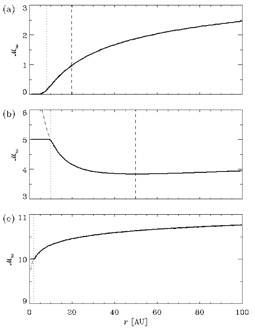
Figure 1: Background wind Mach number $\mathcal{M}_{w}$ as a function of distance $r$ for (a) transonic hydrodynamic wind (model category “T”), (b) supersonic hydrodynamic wind (model category “S”), and (c) wind accelerated by additional $r^{-2}$ force (model category “A”). Thick solid curves show the final stable configuration of the background, following the analytic solution (dot-dashed) outside the conceptual stellar radius $r_{\ast}$ (dotted). Dashed lines in pure hydrodynamic winds indicate the critical radius $r_{c}=GM_{\ast}/2c_{\mathrm{s}}^{2}$ with constant sound speed $c_{\mathrm{s}}$, corresponding to the location of the sonic radius for the transonic branch in (a) and of minimum velocity for supersonic branch in (b).

where $\mathcal{M}_{w}=V_{w}/c_{\mathrm{s}}$ represents the wind Mach number and the critical radius $r_{c}=GM_{\ast}/2c_{\mathrm{s}}^{2}$ is the so-called sonic radius in a transonic wind solution satisfying $\mathcal{M}_{w}(r_{c})=1$. A hydrodynamical wind from the star follows the supersonic ($\mathcal{M}_{w}(r_{c})>1$), transonic ($\mathcal{M}_{w}(r_{c})=1$), or subsonic ($\mathcal{M}_{w}(r_{c})<1$) branch of Parker’s wind solutions (Fig. 1a–b; Lamers & Cassinelli, 1999, see also Figure 3.1 of). Any branch of Parker’s wind solutions shows significant variation of the outflowing velocity inside the critical radius on the scale of a few tens to thousands AU for typical red giant stars (see below for accelerating winds).

The additional outward force due to the stellar radiation pressure on dust, which couples with the gas, is commonly regarded as the wind driving mechanism of AGB stars (Lamers & Cassinelli, 1999; Winters et al., 2000) accelerating the wind faster so that a near-constant velocity is reached at smaller radii. Strong acceleration ($f=1$; $M_{\ast}^{\rm eff}=0$) modifies the isothermal wind to satisfy (see Fig. 1c)

$$\mathcal{M}_{w}^{2}-\mathcal{M}_{w}^{2}(r_{\ast})-2\ln\left(\frac{\mathcal{M}_{w}}{\mathcal{M}_{w}(r_{\ast})}\right)=4\ln\left(\frac{r}{r_{\ast}}\right),$$ (5)

whose quantities are determined by the conditions at the dust condensation radius $r_{\ast}$. In reality, this is probably not a distinct boundary as the wind accelerates gradually and $f$ would not reach unity. Our approximations oversimplify the wind driving mechanism, but‘they are adopted for the background wind condition in order to focus on the larger scale structure.

Although the background wind condition depends on the wind driving mechanism, the response of gas to the gravitational perturbation is insensitive to the global wind structure, but instead is determined by the local wind quantities. This point will be checked by two sets of simulations characterized by the transonic and supersonic branches of Parker’s wind solutions, as well as one set of simulations with $f=1$ mimicking strong radiation pressure. Hence, it will be confirmed that the wake properties are all determined by the wind density $\rho_{w}(r)$, its expansion speed $V_{w}(r)$, and the sound speed $c_{\mathrm{s}}(r)$ on the spot in addition to the orbital and accretion properties of the perturbing substellar mass object.

2.2 Model Parameters

In the background wind characterized by its outflowing velocity $\vec{\mathbf{V_{w}}}$ and corresponding density $\rho_{w}$, we introduce a perturbation $\delta\vec{\mathbf{V}}$ for velocity and $\delta\rho$ for density due to the gravitational potential $\Phi_{p}$ of a substellar companion of mass $M_{p}$ orbiting about the central star at a distance $r_{p}$ with the velocity $V_{p}$. The response of the gaseous medium is governed by the ideal hydrodynamic equations

$$\frac{\partial\rho}{\partial t}+\vec{\mathbf{\nabla}}\cdot(\rho\vec{\mathbf{V}})=0,$$ (6)

and

$$\frac{\partial\vec{\mathbf{V}}}{\partial t}+\vec{\mathbf{V}}\cdot\vec{\mathbf{\nabla}}\vec{\mathbf{V}}=-\frac{c_{\mathrm{s}}^{2}}{\rho}\vec{\mathbf{\nabla}}\rho-\vec{\mathbf{\nabla}}\Phi_{\ast}^{\rm eff}-\vec{\mathbf{\nabla}}\Phi_{p},$$ (7)

for the density $\rho=\rho_{w}+\delta\rho$ and the velocity fields $\vec{\mathbf{V}}=\vec{\mathbf{V_{w}}}+\delta\vec{\mathbf{V}}$. These equations are integrated by the FLASH code of Fryxell et al. (2000) in three dimensional Cartesian coordinates. We utilize the adaptive mesh refinement (AMR) implementation based on the PARAMESH package (MacNeice et al., 1999), in order to minimize the deviations of the wind from a spherical shape by assigning sufficient number of grid cells within $r_{\ast}$ from the center of the mass losing star located at the origin of the Cartesian coordinates. However, to avoid potential artifacts due to the rapidly propagating spiral shocks, the refinement is set only at the beginning of each run such that the nonuniform subgrids are stationary through out the simulation. We use the maximum level of refinement up to eight with the mother grid number of 64$\times$64$\times$32. For the calculation of total gravitational field, the POINTMASS implementation is used with small modifications (1) to include two sources of gravity, (2) to introduce the gravitational softening radii of Plummer-type objects (see, e.g., Binney & Tremaine, 2008), and (3) to allow the motion of the objects.

As the perturber, we consider a substellar mass object with the mass $M_{p}$ greater than 10 $M_{J}$ where $M_{J}$ denotes the mass of Jupiter. The orbit of the perturber is assumed to be circular, ignoring evolutionary processes such as stellar mass loss, mass transport to the substellar object, tidal interaction between the star and the object, and frictional and gravitational drag forces (see, e.g., Villaver & Livio, 2009, and references therein). The range of orbital radius $r_{p}$ considered in our simulations is 10–150 AU. We also confirm that the effect of the perturber size, defined by its gravitational softening radius $r_{s}$, is minor when its size is sufficiently small, exponentially decreasing with decreasing $r_{s}$ (0.1–10 AU). The key parameters are the velocity of the object, $V_{p}$, and of the wind in the outflowing motion $V_{w}$, relative to the sound speed $c_{\mathrm{s}}$. In the numerical simulations, we treat only a pseudo-isothermal gas ($\gamma=1.00001$) with the constant sound speed $c_{\mathrm{s}}$ ranging between 1–10 km s^-1. Given $c_{\mathrm{s}}$, the object speed is arbitrarily selected in the range of $\mathcal{M}_{p}=0.5$–10, to extend parameter space. The wind speeds correspond to a Mach number $\mathcal{M}_{w}<11$. We perform 50 models in total, and Table 1 lists the model parameters of our selected sets of simulations and the respective resolutions. The Bondi accretion radius of the perturber, $r_{B}=GM_{p}/c_{\mathrm{s}}^{2}$, is also listed for reference.

The simulation sets are categorized into accelerated (A), supersonic (S), and transonic (T) background wind models. The S models are further divided according to the wind Mach number into the fast ($\mathcal{M}_{w}=10$) SF and slow ($\mathcal{M}_{w}=5$) SS models. For the A models that treat the wind accelerated by an arbitrary $r^{-2}$ force, we focus on highly supersonic winds, in which the velocity variation is significantly less than that of transonic or marginally supersonic winds, facilitating analysis of the effects of the other parameters explicitly related to the orbiting object. For the S and A models, we start with a constant outflow velocity and a $r^{-2}$ density distribution in the entire domain, and reset the quantities inside $r_{\ast}$ every timestep to avoid the formal infinite values at the center (eqs. [4] and [5]) if an inner boundary is not set. Eventually the flow follows the analytic solution, either equation (4) or (5), determined by the conditions at the reset radius $r_{\ast}$ (Fig. 1). The background density $\rho_{w}$ and velocity field $\vec{\mathbf{V_{w}}}$ for the S and A models are obtained from the separate runs in which the gravitational influence of the perturbing object is suppressed.

3 RESULTS

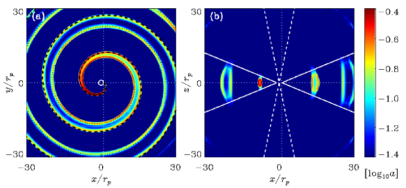
Figure 2: Density enhancement $\alpha$ of model with a fast wind (A1) in logarithmic scale. (a) In the orbital plane, the high density region is bounded by quasi-Archimedes spiral arm boundaries, $r/r_{p}=\varphi\times(\mathcal{M}_{w}\pm 1)/\mathcal{M}_{p}+1$ (black dashed and dotted lines) in the polar coordinates ($r$, $\varphi$) with $\varphi$ measured in the clockwise direction. White solid line represents the circular orbit of the perturbing object moving along in the counterclockwise direction and currently located at the intersection of white dotted lines. (b) In a meridional plane, the wake appears to possess arcs with increasing radius along distance from the center. The boundaries are confined by solid lines having angle of $\tan^{-1}[(\mathcal{M}_{p}^{2}-1)^{1/2}(1+0.2\mathcal{M}_{w}\mathcal{M}_{p})^{-1}]$ from the orbit. The comparison with the extension limit in the absence of wind (i.e., $\mathcal{M}_{w}=0$; dashed) demonstrates the tendency for the wake to vertically flatten with a fast wind. (A color version of this figure is available in the online journal.)

Figure 2 shows the density enhancement factor, $\alpha=\delta\rho/\rho_{w}$, for a fast wind model (A1; see Table 1). Compared to the wakes analyzed in K11 excluding the background wind, the wake in the outflowing environment is radially more extended by $\mathcal{M}_{w}\pm 1$. It is also concentrated to a greater extent toward the orbital plane showing a correlation with both wind and object Mach numbers, $\mathcal{M}_{w}$ and $\mathcal{M}_{p}$. In this section, we elucidate the details of the shape and morphology of the wake pattern in the outflowing circumstance, and determine the arm-interarm density contrast and its dependence on the wind and object properties.

3.1 Shape of Spiral Pattern

The shape of the wake is highly affected by the background flow when formed by the gravitational interaction of the orbiting object with the background medium. In particular, the wake in the wind of an AGB star forms a loosely wound spiral in the orbital plane in contrast to the case of a static medium. The shape of the spiral is determined by the ratio between the pattern propagation speed $V_{\rm arm}$ and the orbital speed of the perturbing object $V_{p}$ (see K11),

$$\frac{d(r/r_{p})}{d\varphi}=\frac{V_{\rm arm}}{V_{p}},$$ (8)

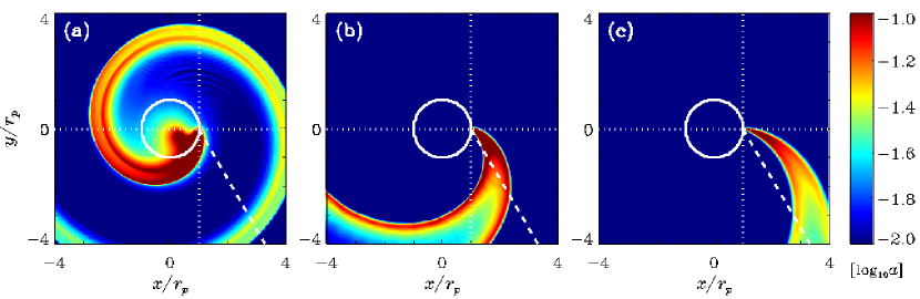
Figure 3: Comparison of the shape of spiral pattern between models with the wind Mach number $\mathcal{M}_{w}$ of (a) 0, (b) 5, and (c) 10. The perturbing object orbits on a circle at distance $r_{p}$ (solid, 20 times greater than the Bondi accretion radius) in the counterclockwise direction with the orbital Mach number $\mathcal{M}_{p}=2$. Its current location is at the intersection of dotted lines. Dashed line denotes the opening angle of the spiral in a static medium, $\Theta=\sin^{-1}\mathcal{M}_{p}^{-1}$, from which the corresponding models with faster winds open up of the spiral pattern. The color bar labels the density enhancement $\alpha$ in logarithmic scale. These models are not listed in Table 1. (A color version of this figure is available in the online journal.)

which reproduces $V_{\rm arm}=c_{\mathrm{s}}$ in Kim & Kim (2007) when the wind is absent. In Figure 3, we compare the spirals induced by the gravitational potential of the orbiting object in different background velocity fields. The change of the spiral shapes due to the different wind velocities is highlighted by the dashed line showing the opening angle of the spiral in a static medium. This line matches the spiral shape in the vicinity of the object in Figure 3a, while the spirals open further with higher wind speeds as displayed in Figure 3b–c. This suggests that, in the presence of wind, the propagation speed of the spiral pattern in the radial direction, $V_{\rm arm}$, is faster than the sonic speed of the medium.

For a linear perturbation analysis, we assume that the wind velocity $V_{w}$ is radial and constant in the entire region (see §2.1 for the background wind conditions applied in numerical simulations). Combining equations (6)–(7) in the linearized versions for the perturbed velocity $\delta\vec{\mathbf{V}}$ under the background conditions satisfying equations (2)–(3), we obtain

$$\frac{D^{2}\vec{\mathbf{\delta V}}}{Dt^{2}}-c_{\mathrm{s}}^{2}\ \vec{\mathbf{\nabla}}\!\left[\left(\vec{\mathbf{\nabla}}-\frac{2}{r}\hat{\mathbf{r}}\right)\cdot\vec{\mathbf{\delta V}}\right]=-\frac{D}{Dt}\vec{\mathbf{\nabla}}\Phi_{p}$$ (9)

where $D/Dt=\partial/\partial t+\vec{\mathbf{V_{w}}}\cdot\vec{\mathbf{\nabla}}$ is the time derivative in the frame moving with the local background wind. Due to the external gravity on the right hand side of the equation, the perturbed gas forms a single-armed spiral-like structure, similar to one in the static background analyzed in detail by K11. Using spherical harmonics for the perturbation, in general, in the form of $\vec{\mathbf{\delta V}}=\vec{\mathbf{\xi}}(r)P_{l}^{m}(\cos\theta)\exp(ikr+im\varphi-i\omega t)$, where $\vec{\mathbf{\xi}}$ is a slowly varying function of radius, we can write

$$\left(\begin{array}[]{lll}(Kr)^{2}-(kr)^{2}&i(kr+i)(A+\cot\theta)&-(kr+i)M\\ iAkr&(Kr)^{2}-L^{2}&iM(A-\cot\theta)\\ -Mkr&iM(A+\cot\theta)&(Kr)^{2}-M^{2}\end{array}\right)\left(\begin{array}[]{l}\xi_{r}\\ \xi_{\theta}\\ \xi_{\varphi}\end{array}\right)=\left(\begin{array}[]{l}0\\ 0\\ 0\end{array}\right),$$ (10)

where $K$, $A$, $M$, and $L^{2}$ are defined as $K=(\omega-V_{w}k)/c_{\mathrm{s}}$, $A=\frac{d}{d\theta}\ln P_{l}^{m}(\cos\theta)$, $M=m/\sin\theta$, and $L^{2}=l(l+1)+(1-m^{2})/\sin^{2}\theta$, respectively. In the WKB approximation ($kr\gg 1$ and $Kr\gg 1$), the dispersion relation yields $\omega=(V_{w}\pm c_{\mathrm{s}})\,k$, indicating that the propagation speed of the pattern is $V_{w}\pm c_{\mathrm{s}}$ at large distances, where $V_{w}$ and $c_{\mathrm{s}}$ are local quantities.

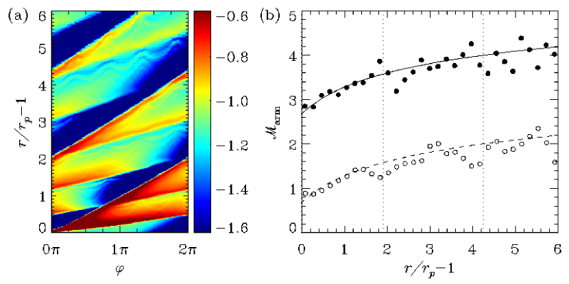
Figure 4: Density enhancement of the spiral structure in logarithmic color scale plotted in the polar coordinates (left), in which the slope of the pattern corresponds to the radial propagation speed of the spiral arm pattern relative to the orbital speed (right) for T model. Solid and dashed lines represent $\mathcal{M}_{w}\pm 1$, tracing the slopes of outer (closed circle) and inner (open circle) boundaries of spiral arm, and the vertical dotted lines denote the turns of outer spiral. (A color version of this figure is available in the online journal.)

In order to check $V_{\rm arm}$ in the numerical simulations, a density map is displayed in Figure 4a for the pattern in polar coordinates ($\varphi,\,r$) in which the slope of the high density arm boundaries represents the velocity ratio $V_{\rm arm}/V_{p}$. Numerical differentiation along the high density boundary indeed gives the propagation speed of $V_{w}+c_{\mathrm{s}}$ for the outer boundary and $V_{w}-c_{\mathrm{s}}$ for the inner boundary (Fig. 4b), depending on the local wind properties and not on the background wind type. This result implies that in the warm central region where the thermal sound speed is relatively large, the shape of spiral must take account of the sound speed as well as the expansion speed of the envelope. The spacing of the arm is not necessarily constant, but varies especially in the wind acceleration zone and in slow wind envelopes. In Figure 4a, the outer boundary reaches $r/r_{p}-1=2.0$ and 4.3 after the first and second turns (see also vertical dotted lines in Fig. 4b) thus the arm spacing increases by 15% (from $\Delta r/r_{p}=2.0$ to 2.3). For the inner boundary, the locations of $r/r_{p}-1=0$, 0.5, 1.2, 2.0, 3.0, 4.2, and 5.4 indicate $\Delta r/r_{p}=0.5$, 0.7, 0.8, 1.0, 1.1, and 1.2 for the respective turns. That is, the arm spacing changes significantly at the first a few turns, where the wind velocity varies considerably in this model, and the increase rate reaches to 140% at the sixth turn relative to the arm spacing at the first turn.

Of particular importance is the overlap of the inner and outer arm boundaries seen in Figure 4a at $r_{\rm over}/r_{p}=1.7$, 3.0, and 5.1. In outflowing envelopes the outer and inner boundaries propagate at different speeds (by $2c_{\mathrm{s}}$), causing overlaps, unlike the unique propagation speed $c_{\mathrm{s}}$ in a static background (K11). Thus the detailed structure of the spiral in the outflowing envelope can be more complicated than in a static background. The difference in propagation speeds results in the overlap of boundaries at resonant positions $r_{\rm over}/r_{p}$ given by the integration of equation (8) as $(V_{w}+c_{\mathrm{s}})/V_{p}\times\varphi$ $\simeq$ $(V_{w}-c_{\mathrm{s}})/V_{p}\times(\varphi+2\pi\times integer)$, assuming that the pattern propagation speed does not change significantly. Hence, the overlap occurs every $\Delta r_{\rm over}$ derived as

$$\frac{\Delta r_{\rm over}}{r_{p}}\simeq\frac{\mathcal{M}_{w}^{2}-1}{\mathcal{M}_{p}}\ \pi,$$ (11)

consistent with the intervals between overlays in Figure 4a.

We should also notice the presence of spiral structures in the cases of subsonic objects (SFx and SSx models). In a static background medium, an object with a subsonic orbital speed ($V_{p}<c_{\mathrm{s}}$) induces the wake to be in a smooth distribution rather than confined within a spiral arm (Kim & Kim, 2007). However, in an outflowing environment, the background wind sweeps and compresses the induced wake material, resulting in a spiral arm shape, as in the cases for supersonic motion.

3.2 Density Enhancement

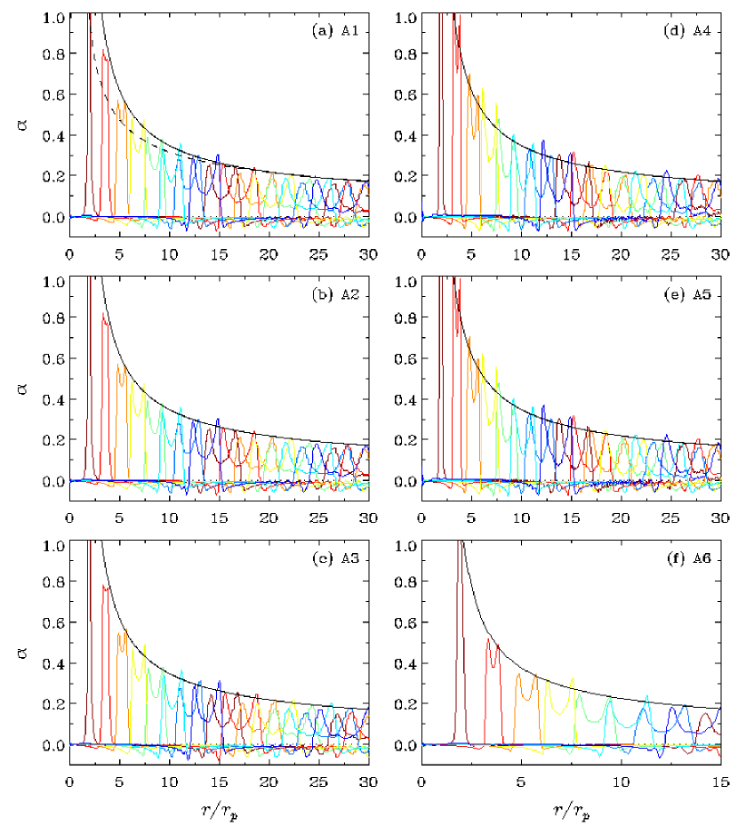
Figure 5: Density enhancement $\alpha$ for models (a) A1, (b) A2, (c) A3, (d) A4, (e) A5, and (f) A6 as a function of the distance normalized by the orbital radius $r_{p}$ of the perturbing object. The colored lines from red to blue display $\alpha$ in the direction apart from the line connecting the object and system center with the angle of 0^∘, 45^∘, 90^∘, 135^∘, 180^∘, 225^∘, 270^∘, and 315^∘ trailing the spiral arm. See text for the formula of the complementary black line that outline the peaks.

Figure 5a exhibits the density enhancement factor for model A1. In order to trace the full structure of the spiral, we plot the profiles along eight different directions in the orbital plane with different colored lines. One noticeable difference from the corresponding profiles in a static background is the level of the zero baseline of the perturbed density. Without a wind, the wake always has minimum density with the central value of $\alpha=r_{B}/r_{p}$ forming a hydrodynamic equilibrium (see K11 for details). However, in the outflowing medium, this global increase of background density is suppressed since the material is swept out of the central part by the wind before its pressure balances the gravitational potential at the central part. This wind sweeping effect also precludes the wake from developing the nonlinear features described by Kim (2010). In Figure 5a, the peak values of the density enhancement decrease with distance as outlined by a solid line (see below). This is approximated by a dashed line, $\alpha=(r_{B}|r-r_{p}|^{-1})^{1/2}$, with the power law index of 0.5 except for the steeper profile in the innermost part.

In order to explore the dependence of the density enhancement $\alpha$ on the properties of object and envelope, we compare in Figure 5 the profiles of $\alpha$ along distances in the orbital plane for the A models. Compared to the fiducial model (A1), we investigate the effects of the stellar mass loss rate $\dot{M_{\ast}}$ (A2), the size of the star $r_{\ast}$ defined by the numerical reset radius (A3), the gravitational softening radius of the perturbing object $r_{s}$ (A4), the mass of the object $M_{p}$ as well as the sound speed of the background gaseous medium $c_{\mathrm{s}}$ (A5), and the orbital radius of the object $r_{p}$ (A6). By comparing model A1 with models A2 and A3, it is found that the perturbed density $\alpha=\delta\rho/\rho_{w}$ does not depend on the mass loss rate $\dot{M_{\ast}}$ and the radius $r_{\ast}$ at which the mass loss occurs, while the overall density structure $\rho_{w}(r)=\dot{M}_{\ast}/4\pi r^{2}V_{w}(r)$ is regulated by the mass loss rate $\dot{M_{\ast}}$ and the background wind velocity $V_{w}(r)$. The independence of density enhancement on the mass loss rate is a natural consequence for an isothermal gas. Reducing the gravitational softening radius $r_{s}$ of the perturbing object by an order of magnitude from $0.1\,r_{B}$ (A1) to $0.01\,r_{B}$ (A4) sharpens the density profiles to some extent but insignificantly changes the overall features. The identity of density profiles in the models A4 and A5 indicates that the density enhancement $\alpha$ depends merely on the Bondi accretion radius $r_{B}\propto M_{p}/c_{\mathrm{s}}^{2}$, and not on the object mass $M_{p}$ or the sound speed $c_{\mathrm{s}}$ individually; it is also checked that $\alpha$ is proportional to $M_{p}$ and $c_{\mathrm{s}}^{-2}$ using models A5-1 and A5-2, respectively. For model A6, the perturbing object is located at a distance twice as large from the central star than the orbital distance in the other A models, resulting in a similar value of $\alpha$ at large distances $r\gg r_{p}$ although the width and interval of the spiral have increased with the larger orbital radius $r_{p}$.

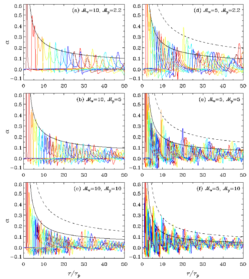
Figure 6: Same as Fig. 5 except for models (a) SFs, (b) SFm, (c) SFf, (d) SSs, (e) SSm, and (f) SSf. The subpattern showing high density groups of peaks (outlined by dashed line) is due to the overlap between the inner and outer boundaries of the spiral wake pattern.

In Figure 6, we further examine the physical parameters that affect the wake density using the S models, focusing on the velocities related to the object motion ($V_{p}$) and the wind expansion ($V_{w}$) in units of background sound speed $c_{\mathrm{s}}$. Comparison between SF models (Fig. 6a–c) and between SS models (Fig. 6d–f) separately reveals a definite anticorrelation of the pattern spacing with the orbital Mach number $\mathcal{M}_{p}$ given a nearly constant wind Mach number $\mathcal{M}_{w}$ (9.5–10 in SF; 3.9–5.2 in SS). On the contrary, one can also find the decrease of the pattern spacing with a smaller wind Mach number $\mathcal{M}_{w}$ by comparing the profiles in (a) and (d), (b) and (e), or (c) and (f). The reduced spacing of the spiral arm pattern facilitates overlaps between the inner and outer arm boundaries characterized by different propagation speeds with respect to each other. As a consequence of the overlaps, the wake develops subpatterns showing additional increases in peak densities at the overlap positions, $r_{\rm over}$, with gradual decreases between the overlap positions. A rough estimate for the overlap intervals, $\Delta r_{\rm over}/r_{p}$ from equation (11), with the assumption of constant $\mathcal{M}_{w}$ is consistent with the intervals between the highest density peaks in Figure 6: $>50$ for (a) and (b), $\sim 30$ for (c), $20-30$ for (d), $10-15$ for (e), and $5-8$ for (f). The peak densities in Figure 6 (excluding the extra peaks due to the subpattern) tend to increase with lower orbital Mach number and higher wind Mach number at $r\gg r_{B}$, albeit the dependence on the wind Mach number is not as clear.

We generalize all the parameter dependence described above, using 50 models of A-, S-, and T-type background winds in the range of $\mathcal{M}_{w}\leq 11$ with $c_{\mathrm{s}}=1$–10 km s^-1 for perturbing objects of $\mathcal{M}_{p}=0.5$–10 and $r_{B}/r_{p}=0.05$–1. By modifying equation (1), based on K11’s analysis for the simpler case of a static uniform background, we obtain an empirical formula for the minimum value of the density peaks (black solid lines in Fig. 5 and 6) described as follows:

$$\alpha_{peak}\gtrsim\frac{r_{B}}{|r-r_{p}|}\left(\frac{\frac{|r-r_{p}|}{r_{B}}\mathcal{M}_{w}^{2}+10\mathcal{M}_{p}\mathcal{M}_{w}+1}{\mathcal{M}_{w}^{2}+|\mathcal{M}_{p}^{2}-1|}\right)^{1/2}\qquad{\rm for}\ \ \mathcal{M}_{w}>1,$$ (12)

which yields $\alpha_{1}$ (eq. [1]) when $\mathcal{M}_{w}=0$. We note that this equation is suitable for supersonic winds since the winds in our simulations are subsonic only in the innermost region in T-type models, which does not sufficiently contribute to the overall profile included in our analysis. A subsonic wind likely leads to a more complicated wake description because (1) it is not able to fully sweep off the delayed perturbations from the object in the past orbits, and (2) concurrently it could cause nonlinear effects, in addition to (3) the wind effect, described here, making the inner and outer arm boundaries overlap because of the different propagating speeds. The dashed lines in Figure 6 outlining the maximum density peaks including substructures, $\alpha=2\alpha_{peak}$ is adopted.

3.3 Vertical Flatness

As seen in Figure 2b, the vertical structure of a gravitational wake has a shape of concentric arcs, confined by solid lines representing the empirical formula for the vertical extension limit. The angular size of the arcs is best fit to the relation

$$\theta_{\rm arc}=2\tan^{-1}\left(\frac{(\mathcal{M}_{p}^{2}-1)^{1/2}}{1+0.2\mathcal{M}_{w}\mathcal{M}_{p}}\right),$$ (13)

which is smaller (or further concentrated toward the orbital plane) in comparison to its counterpart in a static medium ($\mathcal{M}_{w}=0$, dashed; see K11 for details).

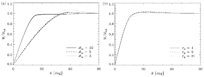
Figure 7: Integrated mass $M$ of perturbed density $\alpha$ as a function of the angle from the orbital plane, normalized by the total mass enhancement $M_{\rm tot}$ in the simulation domain. (a) The integrated mass of wake increases gradually and levels off at 20^∘ for $\mathcal{M}_{w}\simeq 10$ cases (solid, SF models), but it reaches saturation at 50^∘ for $\mathcal{M}_{w}\simeq 3-5$ cases (dashed, SS models; dotted, T model). (b) Comparison of the integrated wake mass in models A1 (dashed), A5-1 (solid), and A5-2 (dotted) indicates its weak dependence on the accretion radius $r_{B}=GM_{p}/c_{\mathrm{s}}^{2}$, and moreover on the perturber mass $M_{p}$ and the sound speed $c_{\mathrm{s}}$ of the gas flow, separately.

In order to quantify the wake mass distribution in the vertical direction, the perturbed density $\alpha$ is integrated as a function of latitudinal angle. Figure 7a displays the integrated wake mass normalized by the total wake mass for different wind Mach numbers $\mathcal{M}_{w}$. The dotted and dashed lines (T and SS models) show gradual increases until reaching unity at $\sim$ 50^∘ for $\mathcal{M}_{w}\simeq 3-5$, while the solid lines (SF models) reveal that the saturation is already achieved at $\sim$ 20^∘ for a higher wind Mach number $\mathcal{M}_{w}\simeq 10$. Beyond these latitudinal angles, the AGB envelopes remain unchanged under the gravitational perturbation of the orbiting substellar object. The decrease of the critical angle with $\mathcal{M}_{w}$ implies a more flattened morphology of the circumstellar matter in a faster outflow. This is due to the fact that in fast background winds, the secondary’s gravitational potential relative to the wind kinematics is low so that its perturbation affects only a limited area. In slow winds, however, the dependence of the vertical extent on $\mathcal{M}_{w}$ is weak, as revealed in the resemblance of the dotted ($\mathcal{M}_{w}=3$) and dashed ($\mathcal{M}_{w}=5$) lines in Figure 7a.

The distribution of the integrated wake mass is relatively independent of $\mathcal{M}_{p}$, $c_{\mathrm{s}}$, $M_{p}$, and the background wind model. For instance, Figure 7a shows the overlap of 4 solid lines (SFf, SFm, SFs, and SFx models) and 4 dashed lines (SSf, SSm, SSs, and SSx models), respectively, for $\mathcal{M}_{p}=0.5$, 2.2, 5.0, and 10.0. The independence on the perturber mass $M_{p}$ and the fluid sound speed $c_{\mathrm{s}}$ (or the Bondi accretion radius $r_{B}$ by association) is shown in Figure 7b (A1, A5-1, and A5-2 models). Moreover, the independence on the wind model is found from similarities between the solid lines in Figure 7a (S models) and the lines in Figure 7b (A models) for fast winds ($\mathcal{M}_{w}\simeq 10$) and between the dotted (T model) and dashed (S models) lines in Figure 7a for slower winds ($\mathcal{M}_{w}\simeq 3-5$). In conclusion, the vertical distribution of a wake in an outflowing background is determined by the Mach number of the average expansion velocity, $\mathcal{M}_{w}$ ($\geq 1$), only weakly depending on the accretion and orbital properties of the perturbing object.

4 DISCUSSION

In order to probe the existence of planets and/or brown dwarfs around evolved giant stars, we investigate the properties of the gravitational wake induced by a substellar mass object in an outflowing environment, through hydrodynamic simulations using the FLASH adaptive mesh refinement code. The perturbing object of substellar mass $M_{p}$ is assumed to be in circular motion at distance $r_{p}$ with the orbital speed of $V_{p}$. For an isothermal sound speed $c_{\mathrm{s}}$, the expansion speed $V_{w}(r)$ of the background wind is determined by the hydrodynamic condition at a reset radius representing the wind-generating location. As functions of the object and wind parameters, $M_{p}$, $r_{p}$, $V_{p}$, $V_{w}$, and $c_{\mathrm{s}}$, we quantify the observable properties of the wake, revealing that the shape of the spiral and arcs are dependent on viewing direction and the density contrast of the structure. Conversely, possible future observations of circumstellar spirals and arcs will allow us to place constraints on the properties of substellar objects in the winds of AGB stars.

We find that the overdense arm pattern of the wake propagates outward with the speed of $V_{\rm arm}=V_{w}\pm c_{\mathrm{s}}$, where the upper and lower signs represent the case for the outer and inner boundaries of the arm pattern, respectively. Here, the speeds are local, implying that the arm spacing varies in the wind acceleration zone and/or in regions where the sound speed varies. In order to measure the variation of arm spacing due to the wind acceleration, which is believed to occur within up to a few tens of stellar radii (Habing & Olofsson, 2003), observations with high angular resolution ($\lesssim$ a few $0.\!\!\arcsec 1$ for the closest AGB stars) are required. Outside the acceleration zone, where the variation of pattern propagation speed is negligible, these pattern propagation speeds yield the wake shape in the orbital plane,

$$r/r_{p}=\varphi\times(V_{w}\pm c_{\mathrm{s}})/V_{p}+1$$ (14)

for the outer and inner boundaries, respectively, constituting Archimedes spiral shapes. If we define the arm spacing $\Delta r_{\rm arm}$ as the interval of the outer or inner boundary individually, the spiral shapes of boundaries simply yield

$$\Delta r_{\rm arm}=(V_{w}\pm c_{\mathrm{s}})\times\frac{2\pi r_{p}}{V_{p}}$$ (15)

assuming that the pattern propagation speed does not significantly vary within one turn. One can estimate the orbital period, $2\pi r_{p}/V_{p}$, by measuring the observed arm spacing in addition to the wind and sound speeds. Alternatively, this is written by

$$\Delta r_{\rm arm}=\frac{2\pi(V_{w}\pm c_{\mathrm{s}})}{(GM_{\ast})^{1/2}}\times r_{p}^{3/2},$$ (16)

from which we can predict the orbital distance $r_{p}$ of the substellar object in the case that the stellar mass $M_{\ast}$ is known. We note that the sound speed should be taken into account especially in a slow wind ($V_{w}\sim c_{\mathrm{s}}$).

The outer arm boundary propagates at a higher speed than the inner boundary by $2c_{\mathrm{s}}$, leading to the broadening of the arm as a function of radial distance. Thus, these high density boundaries overlap each other and are in resonance at the overlap positions, $r_{\rm over}$. Assuming a constant wind and sonic speeds, the spacings of these resonant positions is derived to be $\Delta r_{\rm over}/\Delta r_{\rm arm}=0.5\,(V_{w}/c_{\mathrm{s}}\mp 1)$ (see eqs. [11] and [15]). In cool AGB envelopes, the wind is usually much faster than the sound speed ($V_{w}\gg c_{\mathrm{s}}$), making $\Delta r_{\rm over}$ relatively large. For instance, with $V_{w}=10c_{\mathrm{s}}$, which is easily found for AGB stars, the outer and inner arm boundaries can meet only after five turns. For the case of an observational detection of only parts of the spiral, especially when the partial spiral is expected over the distance of $\Delta r_{\rm over}$, a more careful analysis is required to avoid misidentifying the outer and inner boundaries.

We have also provided an empirical formula (eq. [12]) for the arm-interarm density contrast, $\alpha=\delta\rho/\rho_{w}$, along a normalized distance $r/r_{p}$ as a function of $V_{w}/c_{\mathrm{s}}$, $V_{p}/c_{\mathrm{s}}$, and $r_{B}/r_{p}=GM_{p}/(c_{\mathrm{s}}^{2}r_{p})$. Using this empirical formula, we estimate the properties of a Jupiter wake in the stellar wind when our Sun becomes a giant of size 1 AU ($M_{\ast}=0.8$ $M_{\odot}$, $\dot{M_{\ast}}=2\times 10^{-7}$ $M_{\odot}$ yr^-1, $T_{\ast}=3000K$; according to Hurley et al., 2000). The wind speed $V_{w}$ is set to be $\sim$ 10 km s^-1 based on the trend between the mass-loss rate and the envelope expansion speed (see Fig. 16 in Fong et al., 2006), and the sonic speed $c_{\mathrm{s}}$ is assumed to be 1 km s^-1. The estimated orbital speed $V_{p}=(GM_{\ast}/r_{p})^{1/2}$ of Jupiter in situ ($r_{p}=5$ AU) is 12 km s^-1, corresponding to the arm-interarm density contrast of only 7 % of the background density at distance of 100 AU. The density contrast does not significantly depend on the orbital distance, i.e., 6–11 % for $r_{p}=3$–30 AU. Thus, it is difficult to detect the gravitational wake of a Jupiter mass object with the current observational limitations of sensitivity and angular resolution. In the same range of orbital distance, a 10 Jupiter mass object can create a gravitational wake with the density contrast of 30–44 % at 100 AU; and for a brown dwarf mass (0.07 $M_{\odot}$), the contrast increases to 160–220 %, which may be detectable with the high sensitivity performance of the Atacama Large Millimeter/submillimeter Array (ALMA). We note that these numerical values are lower limits since the peak density contrast at the arm boundary can be higher with a realistic size of the object much smaller than $\geq 0.1$ AU employed in this study; but the effect of the object size $r_{s}$ is not significant unless the size is comparable to the accretion radius $r_{B}$. The required spatial resolution to distinguish the arm pattern separation is 12–370 AU depending on the orbital distance ($r_{p}=3$–30 AU). On a larger scale, a distance corresponding to 5 times this arm separation (in this case of $V_{w}/c_{\mathrm{s}}=10$) is the distance between overlaps showing a higher density contrast by a factor of 2.

The case for fast winds compared to the sonic and object speeds is the most relevant case for many observed AGB envelopes ($\gtrsim$ 10 km s^-1). For a substellar object orbiting at a distance, $r_{p}>10\,(M_{\ast}/M_{\odot})\,(V_{w}/10\,\textrm{km\,s}{}^{-1})^{-2}\,{\rm AU}$, the density contrast at large distance ($r\gg r_{p},\,r_{B}$) can be simply written as

$$\alpha_{peak}\gtrsim\left(\frac{r_{B}}{r}\right)^{1/2}\qquad{\rm for}\ \ V_{w}>V_{p}\gg c_{\mathrm{s}},$$ (17)

from which the measurement of the density contrast provides the value of the Bondi accretion radius $r_{B}=GM_{p}/c_{\mathrm{s}}^{2}$ (or the object mass $M_{p}$ with a given sound speed) for the structure at a known distance from the AGB star. Under the fast wind assumption, the density contrast shows a shallower decrease with distance, compared to its counterpart in an initially static background decreasing as $r^{-1}$ (K11). This shallow decrease in the density contrast facilitates observations at great distances from the star, which is favorable to avoid the high obscuration due to either the bright stellar glare or the dense central environment. Equation (17) indicates that the density contrast between arm and interarm regions can be greater than $\alpha_{peak}$ for distances where

$$\left(\frac{r}{\rm AU}\right)\,\gtrsim\,\left(\frac{M_{p}}{M_{J}}\right)\left(\frac{c_{\mathrm{s}}}{{\rm km\,s}^{-1}}\right)^{-2}{\alpha_{peak}}^{-2}.$$ (18)

Assuming that we can distinguish a density fluctuation of 30 % ($\alpha_{peak}\sim 0.3$), the wake due to an object of mass $M_{p}$ would be observable in the central area within a distance of $\sim 10\,(M_{p}/M_{J})$ AU in the case of $c_{\mathrm{s}}=1$ km s^-1. That is, we may expect to observe the wake of a $10M_{J}$ mass planet within 100 AU with a sensitivity corresponding to a density contrast of 30 %. Alternatively, it may be necessary to take account of the density enhancement due to the planetary wakes when modeling the overall profile of circumstellar envelopes using observational data in which the wakes are not resolved.

In the regime for which the background wind is slower than the orbital velocity ($V_{p}\gtrsim V_{w}\gg c_{\mathrm{s}}$), corresponding to an object in a close orbit at $r_{p}\lesssim 10\,(M_{\ast}/M_{\odot})\,(V_{w}/10\,{\rm km\,s^{-1}})^{-2}\,{\rm AU}$, the peak density contrast at large distance ($r\gg r_{p},\,r_{B}$) is roughly proportional to the velocity ratio $V_{w}/V_{p}$. In this regime, the effect of the wind outflow in opening the spiral pattern competes with the object orbital motion tightening the pattern (see eq. [14]), causing a higher density jump at the more normal shock boundary to the instantaneous flow.

Although the analysis in this paper only treats a substellar mass object orbiting about the AGB star fixed at the system center, our results can be extrapolated to the gravitational density wake of the companion in a stellar binary system. For instance in an AGB envelope, characterized by a temperature of 100 K ($c_{\mathrm{s}}=1$ km s^-1), a solar mass companion would produce a density fluctuation of a factor of 1.6 to 1.3 ($\alpha_{peak}\sim 0.6$–$0.3$ from eq. [17]) at distance of 3,000–10,000 AU from the center of the mass losing star, where the spiral pattern is found in AFGL 3068 (Mauron & Huggins, 2006). The density fluctuation from the companion’s wake is smaller than that estimated from the scattered light observation (the factor of up to $\sim 5$), indicating that the spiral pattern of AFGL 3068 is likely caused by the reflex motion of the AGB star as suggested in Mauron & Huggins (2006), following earlier theoretical work, for example, by Soker (1994). However, in the central 1″ region ($<$ 1,000 AU), where the density fluctuation due to the companion is larger, ALMA would possibly resolve a double spiral structure due to the individual stars. To compare the contribution of the two different mechanisms, we plan to study the density enhancement due to the reflex motion of the mass losing star, similar to the study here. The shapes of two spirals (e.g., pitch angle, arm spacing) are expected to be same, because the spiral shape is determined by the local wind properties, $V_{w}$ and $c_{\mathrm{s}}$. But the spiral of the AGB star is probably detached from the star because of the stellar outflow, contrary to the spiral of the companion attached to the object.

Our work suggests directions for future research. For example, a detailed study of the inner regions of the AGB envelope is necessary to examine the effects of gas heating/cooling, dust anisotropic distribution, and possibly stellar pulsation on the properties of the spiral arm pattern. In addition, investigations of binary systems over a wider range of mass ratios should be examined to explore the modifications in the spiral/arc patterns in the regime where the effect of the reflex motion of the AGB star is also important. Finally, radiative transfer modeling of the molecular line emission and dust continuum are encouraged in order to compare theoretical models with observed structures in detail.

Table 1: Parameters for numerical simulations

	Object Properties						Background Properties					Domain Information
Model	$M_{p}$	$r_{B}$	$r_{s}$	$r_{p}$	$\mathcal{M}_{p}$		$\dot{M}_{\ast}$	$r_{\ast}$	$\overline{\mathcal{M}_{w}}$ ($\mathcal{M}_{w,p}$)	$c_{\mathrm{s}}$		$L$	$\Delta L$	refinement
	[$M_{\odot}$]	[AU]	[AU]	[AU]			[$M_{\odot}$ yr-1]	[AU]		[km s-1]		[AU]	[AU]
Accelerated Wind via $r^{-2}$ Force ($M_{\ast}^{\rm eff}=0$ $M_{\odot}$)
A1	0.01	9	1.0	10	5.0		$1\times 10^{-6}$	2	11 (10.3)	1		300	0.15 – 2.34	7 – 3
A2	0.01	9	1.0	10	5.0		$1\times 10^{-4}$	2	11 (10.3)	1		300	0.15 – 2.34	7 – 3
A3	0.01	9	1.0	10	5.0		$1\times 10^{-6}$	1	11 (10.3)	1		300	0.15 – 2.34	7 – 3
A4	0.01	9	0.1	10	5.0		$1\times 10^{-6}$	2	11 (10.3)	1		300	0.07 – 2.34	8 – 3
A5	0.09	9	0.1	10	5.0		$1\times 10^{-6}$	2	11 (10.3)	3		300	0.07 – 2.34	8 – 3
A5-1	0.01	9	1.0	10	5.0		$1\times 10^{-6}$	2	11 (10.3)	3		300	0.15 – 2.34	7 – 3
A5-2	0.09	9	1.0	10	5.0		$1\times 10^{-6}$	2	11 (10.3)	1		300	0.15 – 2.34	7 – 3
A6	0.01	9	1.0	20	5.0		$1\times 10^{-6}$	2	11 (10.3)	1		600	0.59 – 4.69	6 – 3
Supersonic Wind Branch ($M_{\ast}^{\rm eff}=1$ $M_{\odot}$)
SFf	0.10	10	1.0	20	10.0		$1\times 10^{-6}$	10	10 (9.6)	3		1000	0.98 – 7.81	6 – 3
SFm	0.10	10	1.0	20	5.0		$1\times 10^{-6}$	10	10 (9.6)	3		1000	0.98 – 7.81	6 – 3
SFs	0.10	10	1.0	20	2.2		$1\times 10^{-6}$	10	10 (9.6)	3		1000	0.98 – 7.81	6 – 3
SFx	0.10	10	1.0	20	0.5		$1\times 10^{-6}$	10	10 (9.6)	3		1000	0.98 – 7.81	6 – 3
SSf	0.10	10	1.0	20	10.0		$1\times 10^{-6}$	10	5 (4.2)	3		3000	0.73 – 11.7	8 – 4
SSm	0.10	10	1.0	20	5.0		$1\times 10^{-6}$	10	5 (4.2)	3		3000	0.73 – 11.7	8 – 4
SSs	0.10	10	1.0	20	2.2		$1\times 10^{-6}$	10	5 (4.2)	3		3000	0.73 – 11.7	8 – 4
SSx	0.10	10	1.0	20	0.5		$1\times 10^{-6}$	10	5 (4.2)	3		3000	0.73 – 11.7	8 – 4
Transonic Wind Branch ($M_{\ast}^{\rm eff}=1$ $M_{\odot}$)
T	0.25	25	1.0	100	10.0		$5\times 10^{-5}$	20	3.4 (1.7)	3		2000	0.98 – 15.6	7 – 3

Note. — Each column represents [1] model name, [2] perturbing object’s mass $M_{p}$, [3] Bondi accretion radius $r_{B}=GM_{p}/c_{\mathrm{s}}^{2}$, [4] gravitational softening radius $r_{s}$, [5] orbital radius $r_{p}$, [6] orbital Mach number $\mathcal{M}_{p}$, [7] stellar mass loss rate $\dot{M}_{\ast}$, [8] stellar size $r_{\ast}$ that generates the wind, [9] wind Mach number $\mathcal{M}_{w}$ on average over the simulation domain (and at $r_{p}$), [10] sound speed of background gas $c_{\mathrm{s}}$, [11] half of domain size $L$, [12] range of  spatial resolution $\Delta L$, [13] corresponding range of refinement level with the mother grids of 64$\times$64$\times$32 in $(x,y,z)$-directions. Mass and gravitational softening radius of the central star are 1$M_{\odot}$ and 1 AU, respectively. Underlines emphasize the main difference of the respective models from the fiducial models appearing at the top in categories “A”, “SF”, and “SS”, respectively.

References

- Aikawa & Herbst (1999) Aikawa, Y., & Herbst, E. 1999, A&A, 351, 233
- Binney & Tremaine (2008) Binney, J., & Tremaine, S. 2008, Galactic Dynamics (Princeton, NJ: Princeton Univ. Press)
- Dinh-V.-Trung & Lim (2009) Dinh-V.-Trung, & Lim, J. 2009, ApJ, 701, 292
- Edgar (2004) Edgar, R. 2004, New A Rev., 48, 843
- Edgar et al. (2008) Edgar, R. G., Nordhaus, J., Blackman, E. G., & Frank, A. 2008, ApJ, 675, L101
- Fong et al. (2006) Fong, D., Meixner, M., Sutton, E. C., Zalucha, A., & Welch, W. J. 2006, ApJ, 652, 1626
- Fryxell et al. (2000) Fryxell, B,. Olson, K., Ricker, P., Timmes, F. X., Zingale, M., Lamb, D. Q., MacNeice, P., Rosner, R., Truran, J. W., & Tufo, H. 2000, ApJS, 131, 273
- Fukagawa et al. (2004) Fukagawa, M., et al. 2004, ApJ, 605, L53
- Gilman (1972) Gilman, R. C. 1972, ApJ, 178, 423
- Goldreich & Tremaine (1979) Goldreich, P., & Tremaine, S. 1979, ApJ, 233, 857
- Habing & Olofsson (2003) Habing, H. J., & Olofsson, H. 2003, Asymptotic Giant Branch Stars (New York: Springer)
- Hayashi (1981) Hayashi, C. 1981, Progress of Theoretical Physics Supplement, 70, 35
- He (2007) He, J. H. 2007, A&A, 467, 1081
- Hrivnak et al. (2001) Hrivnak, B. J., Kwok, S., & Su, K. Y. L. 2001, AJ, 121, 2775
- Hurley et al. (2000) Hurley, J. R., Pols, O. R., & Tout, C. A. 2000, MNRAS, 315, 543
- Kim (2011) Kim, H. 2011, ApJ, 739, 102 (K11)
- Kim & Kim (2007) Kim, H., & Kim, W.-T. 2007, ApJ, 665, 432
- Kim & Kim (2009) Kim, H., & Kim, W.-T. 2009, ApJ, 703, 1278
- Kim et al. (2008) Kim, H., Kim, W.-T., & Sánchez-Salcedo, F. J. 2008, ApJ, 679, L33
- Kim (2010) Kim, W.-T. 2010, ApJ, 725, 1069
- Kwok et al. (2001) Kwok, S., Su, K. Y. L., & Stoesz, J. A. 2001, Astrophysics and Space Science Library, 265, 115
- Lafon & Berruyer (1991) Lafon, J.-P. J., & Berruyer, N. 1991, A&A Rev., 2, 249
- Lamers & Cassinelli (1999) Lamers, H. J. G. L. M., & Cassinelli, J. P. 1999, Introduction to Stellar Winds (Cambridge, UK: Cambridge Univ. Press)
- Lin et al. (2006) Lin, S.-Y., Ohashi, N., Lim, J., Ho, P. T. P., Fukagawa, M., & Tamura, M. 2006, ApJ, 645, 1297
- MacNeice et al. (1999) MacNeice, P., Olson, K. M., Mobarry, C., de Fainchtein, R., & Packer, C. 1999, CPC, 126, 3
- Masset (2008) Masset, F. S. 2008, EAS Publications Series, 29, 165
- Mastrodemos & Morris (1999) Mastrodemos, N., & Morris, M. 1999, ApJ, 523, 357
- Mauron & Huggins (1999) Mauron, N., & Huggins, P. J. 1999, A&A, 349, 203
- Mauron & Huggins (2006) Mauron, N., & Huggins, P. J. 2006, A&A, 452, 257
- Morris et al. (2006) Morris, M., Sahai, R., Matthews, K., Cheng, J., Lu, J., Claussen, M., & Sánchez-Contreras, C. 2006, Planetary Nebulae in our Galaxy and Beyond, 234, 469
- Namouni (2010) Namouni, F. 2010, MNRAS, 401, 319
- Ostriker (1999) Ostriker, E. C. 1999, ApJ, 513, 252
- Parker (1958) Parker, E. N. 1958, ApJ, 128, 664
- Sahai et al. (1998) Sahai, R., et al. 1998, ApJ, 493, 301
- Simis et al. (2001) Simis, Y. J. W., Icke, V., & Dominik, C. 2001, A&A, 371, 205
- Soker (1994) Soker, N. 1994, MNRAS, 270, 774
- Villaver & Livio (2009) Villaver, E., & Livio, M. 2009, ApJ, 705, L81
- Willson & Hill (1979) Willson, L. A., & Hill, S. J. 1979, ApJ, 228, 854
- Winters et al. (2000) Winters, J. M., Le Bertre, T., Jeong, K. S., Helling, C., & Sedlmayr, E. 2000, A&A, 361, 641
- Wood (1979) Wood, P. R. 1979, ApJ, 227, 220