From travelling waves to mild chaos: a supercritical bifurcation cascade in pipe flow

Abstract

We study numerically a succession of transitions in pipe Poiseuille flow that leads from simple travelling waves to waves with chaotic time-dependence. The waves at the origin of the bifurcation cascade possess a shift-reflect symmetry and are both axially and azimuthally periodic with wave numbers $\kappa=1.63$ and $n=2$, respectively. As the Reynolds number is increased, successive transitions result in a wide range of time-dependent solutions that includes spiralling, modulated-travelling, modulated-spiralling, doubly-modulated-spiralling and mildly chaotic waves. We show that the latter spring from heteroclinic tangles of the stable and unstable invariant manifolds of two shift-reflect-symmetric modulated-travelling waves. The chaotic set thus produced is confined to a limited range of Reynolds numbers, bounded by the occurrence of manifold tangencies. The states studied here belong to a subspace of discrete symmetry which makes many of the bifurcation and path-following investigations presented technically feasible. However, we expect that most of the phenomenology carries over to the full state-space, thus suggesting a mechanism for the formation and break-up of invariant states that can sustain turbulent dynamics.

1 Introduction

The problem of the transition to turbulence in shear flows is one of great theoretical complexity and paramount practical relevance Grossmann (2000); Eckhardt et al. (2007); Eckhardt (2009). Since Osbourne Reynolds (1883) published his fundamental work on the onset of turbulent motion in a straight pipe of circular cross-section, this problem has become a paradigm for this class of flows. Many theoretical Boberg & Brosa (1988); Brosa & Grossmann (1999), numerical Schmid & Henningson (1994); Zikanov (1996); Shan et al. (1999) and experimental Wygnanski & Champagne (1973); Wygnanski et al. (1975); Darbyshire & Mullin (1995); Hof et al. (2006) studies have focused on elucidating how turbulence can appear for finite amplitude perturbations despite the linear stability of the laminar Hagen-Poiseuille flow Pfenniger (1961); Meseguer & Trefethen (2003).

The computation of finite amplitude solutions in the form of travelling waves Faisst & Eckhardt (2003); Wedin & Kerswell (2004); Pringle & Kerswell (2007) has opened up a window for further studies from a nonlinear dynamics perspective. This parallels similar developments in other flows such as plane Couette Nagata (1997); Wang, Gibson & Waleffe (2007) or plane Poiseuille Pugh & Saffman (1988); Soibelman & Meiron (1991); Ehrenstein & Koch (1991). These waves typically appear in saddle-node bifurcations and come in a variety of symmetries Pringle & Kerswell (2007); Pringle, Duguet & Kerswell (2009). The upper-branch solutions, with wall friction values closer to turbulent ones, seem to play a role in developed turbulence Eckhardt, Schneider, Hof & Westerweel (2007); Kerswell & Tutty (2007); Schneider, Eckhardt & Vollmer (2007) and have been observed in experiments Hof et al. (2004). Their lower-branch counterparts appear to be connected to the critical threshold Duguet, Willis & Kerswell (2008); Mellibovsky & Meseguer (2009) separating the basins of attraction of laminar and turbulent flows, and are relevant for the transition process Skufca et al. (2006); Schneider et al. (2007). Some of the latest developments for the case of pipe flow are compiled in Eckhardt (2009).

The presence of finite amplitude persistent structures is a prerequisite for the appearence of turbulence, but further structural information is needed to explain or understand the dynamics. Specifically, further bifurcations are needed in order to increase the temporal complexity and to change the nature of the dynamics from persistent to transient or vice versa. Accordingly, we here focus on the transitions of these waves in order to explore the origins of the increasing complexity observed in pipe flow.

Since tracking of states with several unstable directions in high-dimensional spaces is technially difficult and computationally demanding, we focus on the subspace with $2$-fold azimuthal periodicity that was also explored in Mellibovsky & Eckhardt (2011). The symmetry eliminates some unstable directions so that a direct identification of the relevant structures without the need for advanced tracking or stabilisation methods is possible. Specifically, we have identified a family of states in this subspace for which the lower-branch solutions have a single unstable direction within the subspace so that a symmetry-restricted time evolution converges when combined with edge tracking techniques Skufca, Yorke & Eckhardt (2006); Schneider, Eckhardt & Yorke (2007); Duguet, Willis & Kerswell (2008); Schneider & Eckhardt (2009). A thorough study of the Takens-Bodganov bifurcation in which this family of waves is created showed that, for wavenumbers beyond a certain value, the upper-branch waves are stable within the subspace and, therefore, within grasp of direct time-evolution Mellibovsky & Eckhardt (2011). We here will study the evolution of the upper branch solutions and their secondary instabilities that lead to time-dependent behaviour and, eventually, to chaos and turbulence.

Due to the broken fore-aft symmetry of pipe flow, the simplest possible solutions already exhibit a time-dependence in the form of an axial downstream drift with a constant phase speed. Some spiralling (rotating-travelling) waves, which rotate due to the breach of all azimuthal reflection ($Z_{2}$) symmetries, have also been identified Pringle & Kerswell (2007); Mellibovsky & Meseguer (2009). Duguet, Pringle & Kerswell (2008) took time-dependency in pipe flow one step further by computing a branch of modulated travelling waves (or, as they called them, relative periodic orbits), although their role in transition or sustained turbulence was assessed as inconclusive. A second family arose naturally from the study of the Takens-Bogdanov bifurcation in Mellibovsky & Eckhardt (2011), but again its existence seemed at best incidental. No further solutions of higher complexity that bridge the gap between the steady laminar flow and turbulence have been observed or computed in pipe flow.

The aim of this study is precisely to take advantage of the stability of upper-branch waves in the family of shift-reflect symmetric states to explore a bifurcating cascade and to produce, along the way, an array of solutions exhibiting ever increasing time-dependent complexity. Figure 1 summarises in a sketch the bifurcation cascade that the travelling waves undergo as Re is increased.

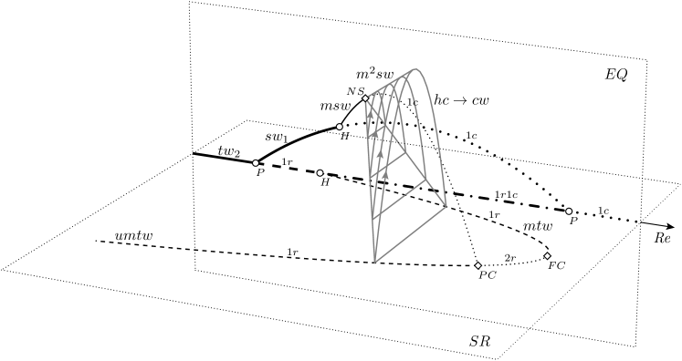
Figure 1: Sketch summarising the bifurcation structure identified and discussed in the present manuscript. The three axes indicate the Reynolds number (Re, the control parameter), the departure from the space of relative equilibria ($EQ$ vertical plane) and the departure from the shift-reflect subspace (horizontal $SR$ plane). The various states found are travelling ($tw$), spiralling ($sw$), modulated-travelling ($mtw$), unstable modulated-travelling ($umtw$), modulated-spiralling ($msw$), doubly-modulated-spiralling ($m^{2}sw$) and chaotic ($cw$) waves. Pitchfork ($P$), Hopf ($H$), Neimark-Sacker ($NS$), fold-of -cycles ($FC$), pitchfork-of-cycles ($PC$), and a global heteroclinic-cyclic ($hc$) bifurcations are indicated. Solid, dashed, dotted and dash-dotted lines represent solutions with $0$ (stable), $1$, $2$ and $3$-dimensional unstable manifolds. Real and complex pairs are indicated with $r$ and $c$.

All relative equilibria ($EQ$ vertical plane) as well as all stable states (solid lines) and part of the shift-reflect ($SR$ horizontal plane) unstable states are readily accessible and give evidence of the bifurcation scenario proposed. We will argue that, at the final stage, the clean heteroclinic-cyclic bifurcation shown here is replaced by a wedge of manifold tangencies giving rise to mildly chaotic waves (as defined and explained in §5).

The states discussed here may be stable in their symmetry-restricted subspace, but they are typically unstable when considered within the full state space. Since there is nothing to suggest that the bifurcation sequence observed and discussed here requires the symmetry reduction (except for reducing the effort that has to go into their identification), it can be expected that it also appears for travelling waves in the full state space. In this sense the present study also suggests paths for the formation and break up of other invariant structures in pipe flow.

The outline of the paper is as follows. In §2, we present the pipe Poiseuille flow problem and sketch a numerical scheme for the integration of the resulting equations. The symmetries of the problem are discussed and numerical methods for the computation and stability analysis of relative equilibria are briefly summarised. Some aspects of bifurcation theory in the case of relative equilibria are also reviewed in §2. A detailed exploration of parameter space delimiting the region of existence of relevant travelling and spiralling waves and an analysis of their stability is presented in §3. In §4 we set out to uncover successive transitions from these waves into increasingly complex types of solutions and describe their main features. The detailed aspects of the global transition leading to the creation of a chaotic set are then discussed in §5. Conclusions and ensuing remarks are summarised in §6.

2 Formulation and methods

In this section we briefly summarise the methods section from a previous contribution so that the symbols and key elements are introduced. Further details can be found in §2 of Mellibovsky & Eckhardt (2011).

We consider the flow of an incompressible Newtonian fluid through a pipe of circular cross section at constant mass flow. The Reynolds number $\mbox{{Re}}=UD/\nu$ is based on the mean axial flow speed $U$, the pipe diameter $D$ and the kinematic viscosity $\nu$. The base profile, in nondimensional cylindrical coordinates ${\mathit{\boldsymbol{x}}}=(r,\theta,z)$, is ${\mathit{\boldsymbol{u}}}_{\rm b}=u_{r}^{\rm b}\;\hat{\mathit{\boldsymbol{r}}}+u_{\theta}^{\rm b}\;\hat{\boldsymbol{\theta}}+u_{z}^{\rm b}\;\hat{\mathit{\boldsymbol{z}}}=(1-r^{2})\;\hat{\mathit{\boldsymbol{z}}}$. The equations for the perturbations in velocity ${\mathit{\boldsymbol{u}}}=(u_{r},u_{\theta},u_{z})$ and pressure $p$ are the Navier-Stokes equations

$$\partial_{t}{\mathit{\boldsymbol{u}}}=-\boldsymbol{\nabla}p+\frac{1}{\mbox{{Re}}}\Delta{\mathit{\boldsymbol{u}}}-({\mathit{\boldsymbol{u}}}\boldsymbol{\cdot}\boldsymbol{\nabla})({\mathit{\boldsymbol{u}}}_{\rm b}+{\mathit{\boldsymbol{u}}})-({\mathit{\boldsymbol{u}}}_{\rm b}\boldsymbol{\cdot}\boldsymbol{\nabla}){\mathit{\boldsymbol{u}}}+f\;\hat{\mathit{\boldsymbol{z}}},\\$$ (1)

together with the incompressibility constraint,

$$\boldsymbol{\nabla}\boldsymbol{\cdot}{\mathit{\boldsymbol{u}}}=0,$$ (2)

the condition for constant mass flux,

$$Q(\mathit{\boldsymbol{u}})=\int_{0}^{2\pi}\int_{0}^{1}(\mathit{\boldsymbol{u}}\boldsymbol{\cdot}\hat{\mathit{\boldsymbol{z}}})\;r{\rm d}r{\rm d}\theta=0,$$ (3)

and the boundary conditions,

$${\mathit{\boldsymbol{u}}}(1,\theta,z;t)={\boldsymbol{0}},\;\;{\mathit{\boldsymbol{u}}}(r,\theta+2\pi/{n_{s}},z,t)={\mathit{\boldsymbol{u}}}(r,\theta,z+2\pi/\kappa,t)={\mathit{\boldsymbol{u}}}(r,\theta,z,t).$$ (4)

The adjustable axial forcing $f=f(t)$ in (1) ensures the constant mass-flux constraint (3). In addition to the non-slip boundary condition at the wall we have periodicity in the azimuthal and axial directions. In the azimuthal direction we take $n_{s}=2$ throughout, confining the analysis to $2$-fold azimuthally-periodic fields. All solutions in this subspace are also solutions to the full Navier-Stokes equations, but the imposed discrete symmetry supresses some undesired unstable directions. The axial wave number $\kappa$ is an additional parameter that was important in unfolding the Takens-Bodganov bifurcation in Mellibovsky & Eckhardt (2011). We here focus on the values $\kappa=1.63$ (${\it\Lambda}\simeq 1.927D$), for which the bifurcation cascade presents its maximum complexity and richness of solutions, and on the interval $\kappa\in[1.5,1.7]$. The Reynolds number is varied in the range $\mbox{{Re}}\in[1800,2800]$, with most of the bifurcations concentrated in a small range around $\mbox{{Re}}\simeq 2200$.

For the spatial discretisation of (1-4) we use a solenoidal spectral Petrov-Galerkin scheme thoroughly described and tested by Meseguer & Mellibovsky (2007). The velocity field is expanded in the form

$$\mathit{\boldsymbol{u}}(r,\theta,z;t)=\sum_{l=-L}^{L}\sum_{n=-N}^{N}{e}^{-{\rm i}(\kappa lz+n_{s}n\theta)}\;\mathit{\boldsymbol{u}}_{ln}(r;t),$$ (5)

$$\mathit{\boldsymbol{u}}_{ln}(r;t)=\sum_{m=0}^{M}a_{lnm}^{(1,2)}(t)\;\mathit{\boldsymbol{v}}_{lnm}^{(1,2)}(r),$$ (6)

with $a_{lnm}^{(1,2)}$ the complex expansion coefficients which are collected in a state vector $\mathit{\boldsymbol{a}}$. The spectral resolution, checked as adequate for the computations performed in this study, has been set to $L=16$, $N=12$ and $M=36$, corresponding to $\pm 16$ axial and $\pm 12$ azimuthal Fourier modes, and to $37$ Chebyshev collocation points for the radial coordinate. For the time-evolution, we take a 4th order linearly implicit method with stepsize $\Delta t=1\times 10^{-2}\,D/(4U)$.

Fluid flow solutions lie in infinite dimensional space, of which we compute finite, yet high-dimensional representations. Elegant approaches to project these solutions onto low-dimensional spaces to aid visualisation have been devised Gibson, Halcrow & Cvitanović (2008) and successfully applied to other flows such as plane Couette Gibson, Halcrow & Cvitanović (2009). We take the simpler approach of using some random expansion coefficients and global derived quantities to represent the flow. To free the representation from the drifting degeneracy associated to the travelling and/or rotating component of the waves, it is more convenient to use the absolute value rather than the coefficients themselves. In this study we will be making extensive use of the moduli of a streamwise-independent ($\lvert a_{010}^{(2)}\rvert$), an axisymmetric ($\lvert a_{100}^{(2)}\rvert$) and a mixed ($\lvert a_{110}^{(2)}\rvert$) coefficient. In what follows, the absolute value symbols will be omitted for simplicity.

The basic solutions come in the form of travelling waves, which are best described as relative equilibria and possess the continuous space-time symmetry

$$(u,v,w)_{\rm tw}(r,\theta,z;t)=(u,v,w)_{\rm tw}(r,\theta,z-c_{z}t;0),$$ (7)

where $c_{z}$ is the axial drift speed. In a comoving reference frame travelling downstream with speed $c_{z}$ travelling waves appear as stationary solutions. Near a relative equilibrium the drift dynamics is trivial and decouples from the dynamics orthogonal to the drift. As a result, bifurcations of relative equilibria can be analysed in two steps, first describing the bifurcations associated to the orthogonal dynamics, then adding the corresponding drift along the travelling direction Krupa (1990).

In order to avoid the transformation to the co-moving frame of reference, it is convenient to have observables that are translationally invariant in the axial direction: then the phase motion of the travelling wave drops out and they appear as fixed points in this observable without further action. One such quantity is the normalised energy,

$$\varepsilon({\mathit{\boldsymbol{u}}})=\frac{1}{2\epsilon_{\rm b}}\int_{0}^{2\pi/\kappa}{\rm d}z\int_{0}^{2\pi}{\rm d}\theta\int_{0}^{1}r{\rm d}r\;{\mathit{\boldsymbol{u}}}^{*}\boldsymbol{\cdot}{\mathit{\boldsymbol{u}}},$$ (8)

with $\epsilon_{\rm b}=\pi^{2}/(3\kappa)$ the energy of the basic flow and ^∗ symbolising complex conjugation. This energy decouples exactly into the sum of its axial-azimuthal Fourier components $\varepsilon_{ln}=\varepsilon(\mathit{\boldsymbol{u}}_{ln})$. As a measure of three-dimensional structure, we define the non-axisymmetric streamwise-dependent component as $\varepsilon_{\rm 3D}=\sum_{l,n\neq 0}\varepsilon(\mathit{\boldsymbol{u}}_{ln})$.

Another such quantity is the mean axial pressure gradient needed to drive the flow at constant mass-flux, normalised by the pressure gradient for the corresponding laminar flow,

$$(\boldsymbol{\nabla}p)_{z}=\left.\left\langle\iint_{r,\theta}\frac{\partial p}{\partial z}\right\rangle_{z}\right/\left(\frac{dp}{dz}\right)_{lam}=1+\frac{Ref}{4}.$$ (9)

It is closely related to the wall friction factor Schlichting & Gersten (2000):

$$C_{f}=\frac{2D}{\rho U^{2}}\left\langle\iint_{r,\theta}\frac{\partial p}{\partial z}\right\rangle_{z}=64\frac{(\boldsymbol{\nabla}p)_{z}}{Re},$$ (10)

which constitutes a good indicator of whether the flow is laminar or turbulent.

In the azimuthal direction, all the solutions studied here are invariant under the cyclic group $C_{2}$ (rotations by integer multiples of $\pi$). On top of this symmetry, the travelling wave family that constitutes the departing point for the present study, possesses an additional discrete symmetry: a combined shift-reflect symmetry. Solutions invariant under this symmetry operation,

$$S{\mathit{\boldsymbol{u}}}({\mathit{\boldsymbol{x}}})=S(u,v,w)(r,\theta_{i}+\theta,z;t)=(u,-v,w)(r,\theta_{i}-\theta,z+\pi/\kappa;t),$$ (11)

are left unaltered when shifted half a wavelength downstream and then reflected with respect to any of two diametral planes tilted with $\theta_{0}$ and $\theta_{0}+\pi/2$, where $\theta_{0}$ parametrises the azimuthal degeneracy of solutions. It can be shown that the expansion coefficient $a_{100}^{(2)}$ vanishes exactly when this symmetry is present, its norm giving a fairly good notion of how far apart from the symmetry space any given flow field is. The $S$ symmetry is a remnant version of the $Z_{2}$ reflections group implied by the broken $O(2)=SO(2)\times Z_{2}$ azimuthal symmetry. Waves that break all left-right symmetries incorporate an azimuthal precessing motion on top of the axial drift, so that they spiral and modify (7) into

$$(u,v,w)_{\rm tw}(r,\theta,z;t)=(u,v,w)_{\rm tw}(r,\theta-c_{\theta}t,z-c_{z}t;0),$$ (12)

where $c_{\theta}$ is the azimuthal drift speed. Evidently, the decoupling from the drift dynamics of the drift-orthogonal dynamics discussed for travelling waves holds true for waves that also rotate.

Modulated waves arise from Hopf bifurcations of travelling and spiralling waves. No general result is available when it comes to their stability. The effects on the degenerate frequency (or frequencies) associated to the travelling (or spiralling) component of the wave when a modulational frequency comes into play cannot be discarded at once. Nonetheless, as our computations will show, the approach of choosing an appropriate comoving frame of reference remains accurate, and modulated travelling (spiralling) waves seem to behave as relative periodic orbits rather than as generic quasiperiodic orbits on a $2$-torus ($3$-torus).

In order to choose this appropriate frame of reference we define the instantaneous axial and azimuthal phase speeds Mellibovsky & Eckhardt (2011) as the values $c_{z}$ and $c_{\theta}$, respectively, that minimize at any given instant of time, the $2$-norm

$$\min_{c_{z},c_{\theta}}\left\|\mathit{\boldsymbol{a}}(t+\Delta t)-\mathsfbi{T}(c_{z}\Delta t)\mathsfbi{R}(c_{\theta}\Delta t)\;\mathit{\boldsymbol{a}}(t)\right\|,$$ (13)

with $\mathsfbi{T}(\Delta z)$ and $\mathsfbi{R}(\Delta\theta)$ the diagonal operators for translation and rotation, whose action on the components of the state vector is defined as:

$$\left.\begin{array}[]{rcl}\left(\mathsfbi{T}(\Delta z)\;\mathit{\boldsymbol{a}}\right)_{lnm}^{(1,2)}&=&a_{lnm}^{(1,2)}\;\mathrm{e}^{-{\rm i}\kappa l\Delta z},\\[5.69046pt] \left(\mathsfbi{R}(\Delta\theta)\;\mathit{\boldsymbol{a}}\right)_{lnm}^{(1,2)}&=&a_{lnm}^{(1,2)}\;\mathrm{e}^{-{\rm i}n_{s}n\Delta\theta}.\end{array}\right\}$$ (14)

Therefore, we will systematically work on a comoving reference frame in which waves become equilibria and we will apply continuous dynamical systems theory. Moreover, modulated and doubly-modulated waves become periodic orbits and $2$-tori, so that they can be seen as equilibria and periodic orbits, respectively, on a purposefully designed comoving Poincaré section. This is accomplished by using drift-independent quantities upon definition of the Poincaré section. The stability of modulated waves can then be studied through their associated Poincaré map, making use of discrete-time dynamical systems theory.

Besides the complications introduced by the bifurcation of relative equilibria, i.e. group orbits invariant under the flow of equivariant vector fields, we will be dealing here with additional symmetries that modify or replace well known bifurcating scenarios that are typical of low dimensional dynamical systems. To overcome this, we will take advantage of the substantial developments that have been achieved in the last two decades regarding bifurcation in dynamical systems with symmetries Golubitsky, Stewart & Schaeffer (1988); Crawford & Knobloch (1991); Chossat & Lauterbach (2000).

3 Relative equilibria

The relative equilibria considered here are travelling waves or spiralling waves, i.e. states that become stationary in appropriately translating and/or rotating frames of reference. In addition to the discrete $2$-fold azimuthal periodicity ($C_{2}$, i.e. $n_{s}=2$), the waves at the origin of this study also show a combined shift-reflect symmetry ($S$). They were first computed by Faisst & Eckhardt (2003) and Wedin & Kerswell (2004) using volume forcing homotopy.

When parametrised in terms of axial wavenumber ($\kappa$) and Reynolds number (Re), they appear in a Takens-Bogdanov bifurcation, thoroughly studied in Mellibovsky & Eckhardt (2011). Their existence extends in Reynolds number to as low as $\mbox{{Re}}\simeq 1358.5$ for the optimal wave number $\kappa\simeq 1.55$ Faisst & Eckhardt (2003); Wedin & Kerswell (2004). Ensuing from this bifurcation scenario there are parameter regions in which upper-branch solutions are stable to $2$-fold azimuthally-periodic perturbations so that time-dependent solutions which bifurcate at higher Re can be computed via straightforward symmetry-restricted time-evolution.

In what follows, we continue both upper- and lower-branch members of this family of travelling waves to higher Re and analyse their stability in order to explore the framework in which increasingly complex dynamics occur.

We do not study the shift-reflect mirror-symmetric family of travelling waves Duguet et al. (2008) that coexists in state space with the solutions discussed here. They reside in a region of phase space that is noticeably far from the present region of interest and there are no indications that they interact with the solutions found in this work, at least not in the parameter ranges studied here.

3.1 Travelling waves

Lower-branch travelling waves of this family can be continued to extremely high Re without much noticeable change to their stability properties, regardless of $\kappa$. As many other lower-branch travelling waves, they seem to develop a critical layer as Re is increased Viswanath (2009) and exhibit a single unstable eigenmode when considered in the azimuthal subspace they inhabit. They are edge states Schneider et al. (2007) of the $2$-fold azimuthally-periodic pipe within this subspace. In the full state space they may be part of the edge and may provide the symmetric states needed to connect the stable manifolds of non-symmetric but symmetry-related edge states Vollmer, Schneider & Eckhardt (2009). Figure 2(a) shows $z$-averaged cross-sectional axial velocity contours ($\langle u_{z}\rangle_{z}$, left) and a couple of axial vorticity isosurfaces ($\omega_{z}$, right) of a lower-branch travelling wave at $(\kappa,\mbox{{Re}})=(1.63,2215)$.

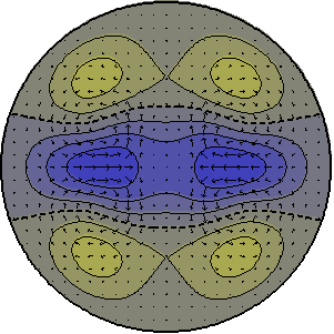
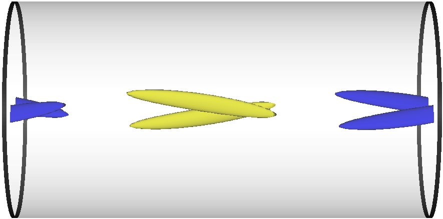
(a)			(b)
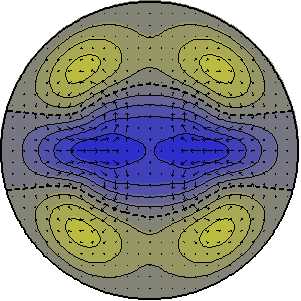
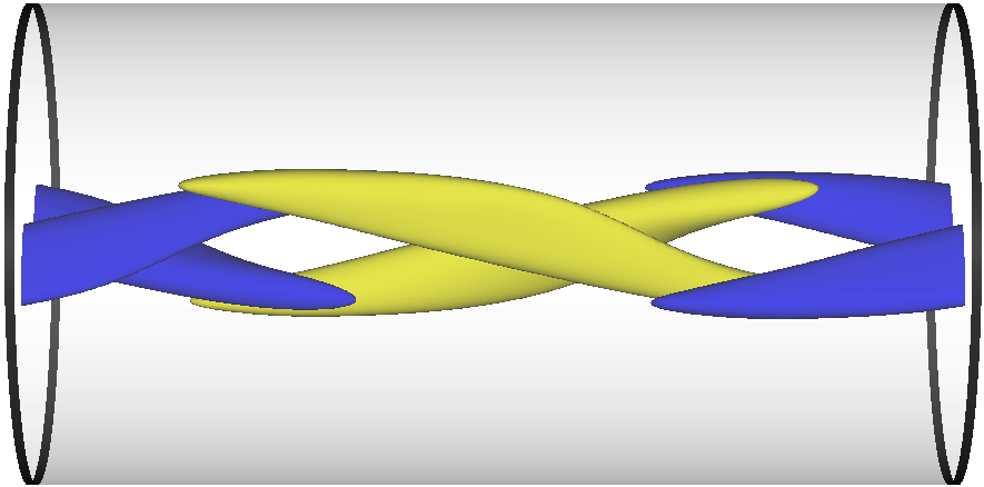
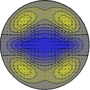
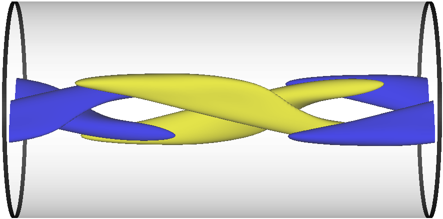
(c)			(d)

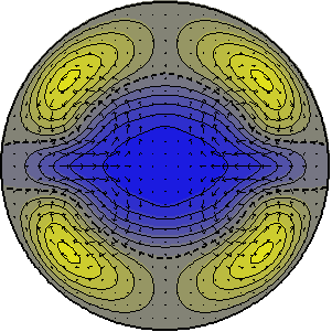
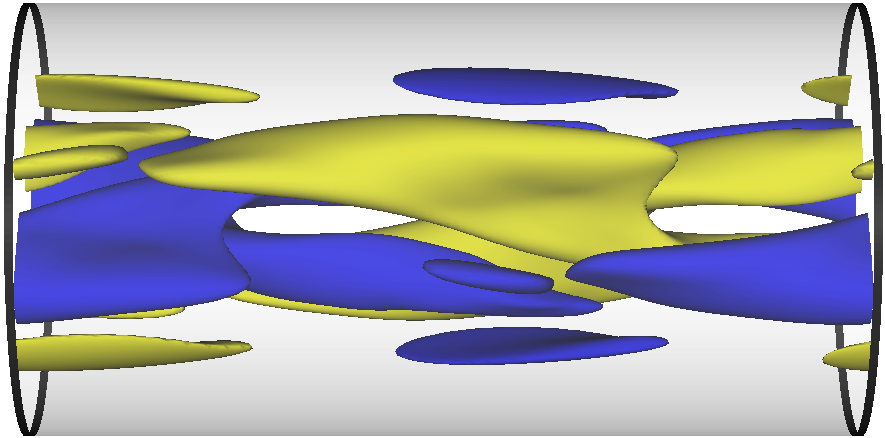
Figure 2: Travelling waves at $(\kappa,\mbox{{Re}})=(1.63,2215)$. Left: $z$-averaged cross-sectional axial velocity contours spaced at intervals of $\Delta\langle u_{z}\rangle_{z}=0.1U$. In-plane velocity vectors are also displayed. Right: axial vorticity isosurfaces at $\omega_{z}=\pm 1U/D$. Fluid flows rightwards. Blue (dark gray) for negative, Yellow (light) for positive. (a) Lower-branch ($tw_{1}$), (b) lower-middle-branch ($tw_{2}$), (c) upper-middle-branch ($tw_{3}$) and (d) upper-branch ($tw_{4}$) travelling waves.

The shift-reflect symmetry of the solution is evidenced by the two orthogonal diametral reflection planes (at $\theta_{i}=0,\pi/2$) of the $z$-averaged cross-sectional contours. High- and low-speed streaks are clearly visible. In-plane velocity vectors show the location, on average, of the two pairs of counter-rotating vortices that are displayed in the three-dimensional view.

The behaviour of upper-branch waves depends much more strongly on $\kappa$. This is apparent from figure 3, where $(\boldsymbol{\nabla}p)_{z}$ has been plotted against Re for three different values of $\kappa$.

(a)
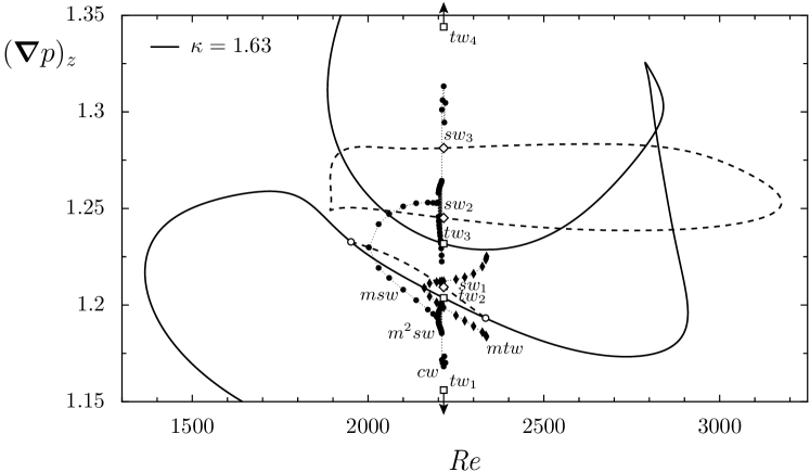
(b)

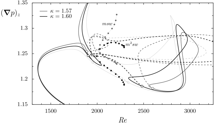
Figure 3: Mean axial pressure gradient ($(\boldsymbol{\nabla}p)_{z}$) as a function of Re for (a) $\kappa=1.63$ and (b) $\kappa=1.57,1.60$ (shading as explained in the legend). Solid lines represent shift-reflect travelling waves, dashed for spiralling waves. Extrema of time-dependent travelling/spiralling solutions are marked as filled diamonds/circles, which denote Hopf bifurcations when placed on equilibria continuation curves. Open circles denote pitchfork bifurcations. Relative equilibria at $(\kappa,\mbox{{Re}})=(1.63,2215)$ have been marked with open squares ($tw_{s}$, travelling waves from figure 2) and diamonds ($sw_{s}$, spiralling waves from figure 6). Modulated travelling, modulated spiralling, doubly-modulated spiralling and chaotic waves are labelled $mtw$, $msw$, $m^{2}sw$ and $cw$, respectively.

At high $\kappa$ (figure 3a), upper-branch waves extend to moderate $\mbox{{Re}}\sim 2900$, then turn back in a contorted fashion toward lower values of the parameter, undergo a saddle-node bifurcation at about $\mbox{{Re}}\simeq 1885$ and finally progress towards much higher Re. As a result, four instances of the same solution coexist over a fairly wide Re-range. They are shown in figure 2 for $(\kappa,\mbox{{Re}})=(1.63,2215)$ and marked with open squares as $tw_{1}$, $tw_{2}$, $tw_{3}$, and $tw_{4}$ in figure 3(a). As already mentioned, the wave requiring the lowest driving axial pressure gradient ($tw_{1}$, on the lower branch, out of scale in figure 3a for clarity) lives on the laminar flow basin boundary. At the other end of the continuation curve, the waves exhibit driving pressure gradients in the region of turbulent flow values ($tw_{4}$, figure 2d, on the upper branch, also out of range in figure 3a)). Structures resembling these and other upper-branch travelling waves have been observed experimentally in developed turbulence Hof et al. (2004) as well as in numerical simulation Kerswell & Tutty (2007); Schneider, Eckhardt & Vollmer (2007); Willis & Kerswell (2008). The shift-reflect symmetry is clearly preserved but vorticity and axial velocity gradients in the vicinity of the wall are much more pronounced than for the lower-branch waves, as expected for turbulent solutions.

Due to the contorted shape of the curve, two additional waves exist in a region that extends up to $\mbox{{Re}}\simeq 2800$. They are $tw_{2}$ and $tw_{3}$ of figures 2b and 2c, which we dub lower- and upper-middle-branch waves, respectively, because of the relative values of their pressure gradients. Both waves are also shift-reflect symmetric. The main properties of all members of this travelling-waves family at $(\kappa,\mbox{{Re}})=(1.63,2215)$ are summarised in table 1.

	$(\boldsymbol{\nabla}p)_{z}$	$\nu$	$c_{z}$	$10^{3}\times c_{\theta}$	$10^{4}\times\varepsilon_{\rm 2\theta}$	$10^{2}\times\varepsilon_{\rm 2z}$	$10^{4}\times\varepsilon_{\rm 3D}$	$ev\in S$	$ev\in\bar{S}$
$tw_{1}$	$1.1171$	$0.03228$	$1.5481$	$0.0$	$0.3940$	$1.0508$	$4.0964$	$1r$
$tw_{2}$	$1.2037$	$0.03478$	$1.4600$	$0.0$	$1.0010$	$1.3027$	$7.5781$	$1c$	$1r$
$tw_{3}$	$1.2318$	$0.03559$	$1.4349$	$0.0$	$1.3086$	$1.3051$	$8.8704$	$1r$	$1r$
$tw_{4}$	$1.4738$	$0.04258$	$1.2891$	$0.0$	$4.3161$	$1.4333$	$19.280$	$1c$	$1r+2c$
$sw_{1}$	$1.2093$	$0.03494$	$1.4583$	$\pm 0.9192$	$1.0331$	$1.3632$	$7.6261$		$1c$
$sw_{2}$	$1.2813$	$0.03702$	$1.4413$	$\pm 1.5964$	$1.6748$	$1.9689$	$8.4999$		$1r+1c$
$sw_{3}$	$1.2451$	$0.03597$	$1.5015$	$\pm 1.9248$	$1.7667$	$2.4578$	$5.3584$		$1c$

Table 1: Relative equilibria of the $2$-fold azimuthally periodic subspace at $(\kappa,\mbox{{Re}})=(1.63,2215)$. The last two columns, $ev\in S$ and $ev\in\bar{S}$, count real ($r$) and complex pairs ($c$) of eigenmodes corresponding to the shift-reflect and shift-reflect-orthogonal subspaces, respectively. Tabulated travelling/spiralling waves are marked with open squares/diamonds in figure 3(a).

For lower $\kappa$ (figure 3b), the continuation curve splits into two, adding two extra saddle-node points and leaving an island of solutions at moderate Re. Figure 4 shows a close-up of the parameter region where this topological change takes place.

(a)

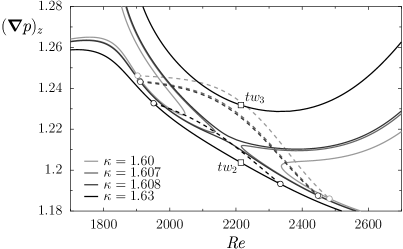
(b)

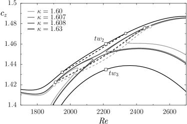
Figure 4: Detail near $(\kappa,\mbox{{Re}})\sim(1.61,2200)$ highlighting the change in behaviour of the continuation curves. Solid lines represent travelling waves (darker for increasing $\kappa$) whereas dashed lines correspond to spiralling waves. Lower-middle branch ($tw_{2}$) and upper-middle branch ($tw_{3}$) waves are indicated with squares. Open circles denote pitchfork bifurcations. (a) Mean axial pressure gradient $(\boldsymbol{\nabla}p)_{z}$ and (b) axial advection speed ($c_{z}$), as a function of Re.

It becomes clear in figure 4(a) that for $\kappa\lesssim 1.607$, the segments of the continuation curve corresponding to $tw_{2}$ and $tw_{3}$ collide and produce a gap in Re where the multiplicity of solutions is reduced to just two. Waves $tw_{2}$ and $tw_{3}$ at $(\kappa,\mbox{{Re}})=(1.63,2215)$ (figures 2b,c) already look much alike and, indeed, collide in a saddle-node point and disappear as $\kappa$ is reduced, leaving $tw_{1}$ and $tw_{4}$ (figures 2a,d) as the only surviving members of the family.

3.2 Spiralling waves

A pair of symmetry-conjugate branches of spiralling waves branches off the lower-middle-branch of shift-reflect waves in a symmetry-breaking pitchfork bifurcation (dashed lines in figures 3 and 4a,b). As a result of the loss of symmetry they start precessing in the azimuthal direction, but remain stationary in an appropriately spiralling frame of reference.

For the lower $\kappa$ shown (light gray), the Re-continuation curve starts at a pitchfork point, exhibits a counterclockwise loop to higher values of the pressure gradient and then a clockwise loop to lower pressure gradients before continuing to higher Re. The branch extends beyond the region of existence of middle-branch travelling waves, where it exhibits an additional fold (outside the range of the figure) that takes them back in Re. At this point the curve bends back to end up branching back with middle-branch travelling waves in a second pitchfork. In this way, the spiralling waves bridge the Re-gap left by middle-branch travelling waves described above. At the two pitchfork ends of the continuation curve, spiralling waves bifurcate with no rotation speed. As the asymmetry increases, rotation speed builds up reaching significant precessing rates, as shown in figure 5.

(a)

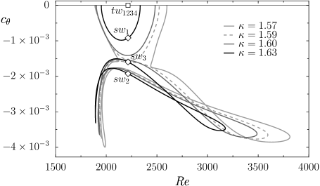
(b)

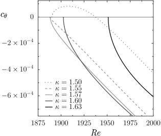
Figure 5: (a) Rotation phase speed ($c_{\theta}$) as a function of Re and $\kappa$ (shading) for spiralling waves. Shift-reflect travelling waves collapse on the $x$-axis. Relative equilibria at $(\kappa,\mbox{{Re}})=(1.63,2215)$ have been marked with open squares ($tw_{s}$, travelling waves from figure 2) and diamonds ($sw_{s}$, spiralling waves from figure 6). (b) Detail of the bifurcating point including lower $\kappa$-curves.

The waves continued have negative rotation speed, but, obviously, their shift-reflected counterparts exhibit opposite azimuthal rotation. The rotation drift of the waves is much slower than their axial drift. As a matter of fact, the spiralling waves reported here travel a minimum of $700$ wavelengths or $1350$ diameters in the time they complete a full rotation.

For $\kappa\gtrsim 1.59$ (dashed curve in figure 5a) the continuation curve splits in two, leaving a disconnected island of strongly spiralling waves and a monotonous curve connecting at both ends with the travelling-wave family. At $(\kappa,\mbox{{Re}})=(1.63,2215)$, three different spiralling waves coexist: lower-, middle- and upper-branch waves, indicated by open diamonds and named $sw_{1}$, $sw_{2}$ and $sw_{3}$. They are shown in figure 6 and they all clearly break the shift-reflect symmetry.

(a)
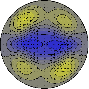
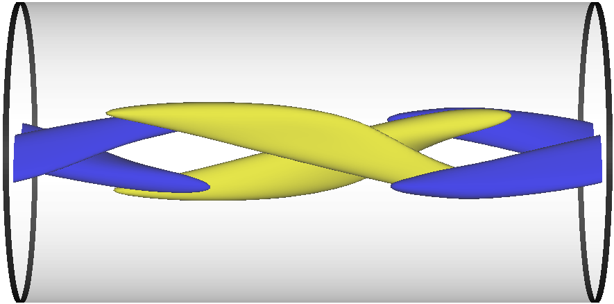
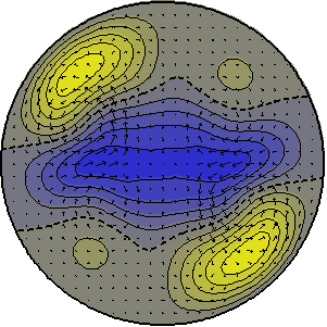
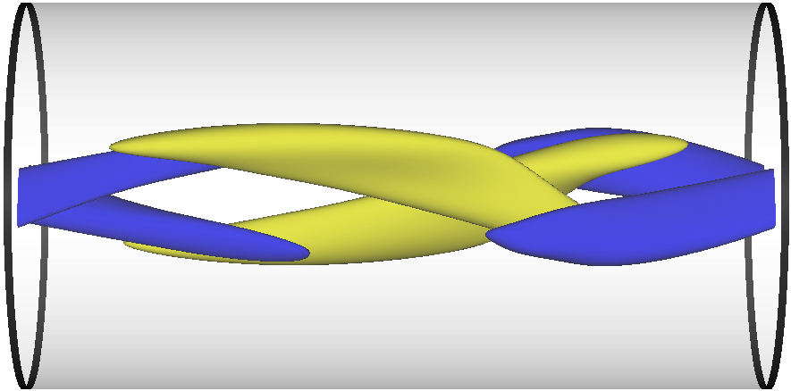
(b)			(c)

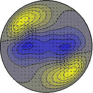
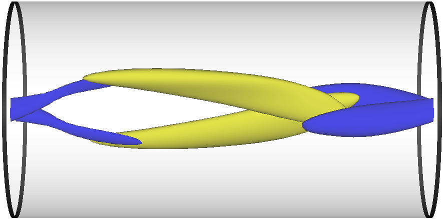
Figure 6: Spiralling waves at $(\kappa,\mbox{{Re}})=(1.63,2215)$. Left: $z$-averaged cross-sectional axial velocity contours spaced at intervals of $\Delta\langle u_{z}\rangle_{z}=0.1U$. In-plane velocity vectors are also displayed. Right: axial vorticity isosurfaces at $\omega_{z}=\pm 1U/D$. Fluid flows rightwards. Blue (dark gray) for negative, yellow (light) for positive. (a) Lower-branch ($sw_{1}$), (b) middle-branch ($sw_{2}$) and (c) upper-branch ($sw_{3}$) spiralling waves.

The spiralling waves most strongly related to $tw_{2}$ is $sw_{1}$. They are close in parameter space (their continuation curves are connected) and they also look very much alike. Cross-sectional contours are strikingly similar, except that $sw_{1}$ has slightly broken the shift-reflect symmetry. The other two spiralling waves, $sw_{2}$ and $sw_{3}$, have completely broken the symmetry and their rotation rates are much larger than for $sw_{1}$. The main properties of these spiralling waves at $(\kappa,\mbox{{Re}})=(1.63,2215)$ are summarised alongside those of travelling waves in table 1.

It has already been pointed out that spiralling waves that break a left-right symmetry, here in the form of a shift-reflect symmetry, appear in symmetry-related pairs that rotate either clockwise or counterclockwise with opposite rotation speeds. This is a general remark, but the loss of symmetry does not preclude the existence of non-robust asymmetric waves that balance the azimuthal driving force and, consequently, do not rotate. As is the case for some helical waves in pipe flow Pringle & Kerswell (2007), non-shift-reflect waves exist whose rotation rate cancels exactly. This is exemplified for $\kappa=1.50$ (dotted line) in figure 5(b), where a branch of spiralling waves first appears with counterclockwise rotation that only for higher Reynolds numbers switches to the clockwise rotation that characterises all other spiralling waves continued in the plot. As the rotation speed crosses zero, two mutually-symmetric spiralling waves switch the sense of rotation. Since this crossing happens for a specific value of the system parameters it is a non-robust, non-generic phenomenon.

3.3 Stability of travelling and spiralling waves

The Takens-Bogdanov bifurcation in which the travelling waves appear at the lower Re-range was studied in Mellibovsky & Eckhardt (2011). Lower-branch waves were shown to always exhibit a single unstable direction, while sufficiently far away from the bifurcation point, upper-branch waves (here renamed lower-middle-branch for convenience) were shown to be stable to all $2$-fold azimuthally-periodic perturbations.

The stability properties of travelling waves along the continuation surface is quite involved, with many eigenvalues crossing back and forth, and many states related by the multiple folds present. A detailed study of these bifurcations is beyond the scope of the present analysis. Instead, we will concentrate on parameter regions where interesting dynamics occur and on stable waves that transitions to more complex flows. Thus, we will initially keep the wavenumber at $\kappa=1.63$ and search for bifurcations of the lower-middle-branch travelling wave ($tw_{2}$) and the lower-branch spiralling wave ($sw_{1}$) with Reynolds numbers in the range $\mbox{{Re}}\in[1800,2600]$. Stability of other waves will be reported for completeness, but their transitions cannot be analysed in detail since the states resulting are all unstable at onset and not accessible through time evolution. The stability analysis will then be broadened by varying $\kappa$ and Re together in order to extend the bifurcation points into bifurcation curves in $(\mbox{{Re}},\kappa)$-parameter space.

Figure 7(a) tracks the relevant (bifurcating) eigenvalues of $tw_{2}$ and $sw_{1}$ for $\kappa=1.63$ and varying Re.

(a)

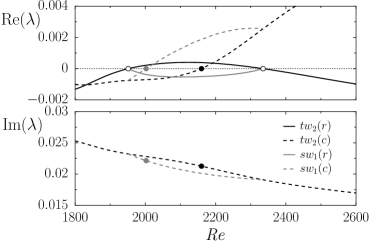
(b)

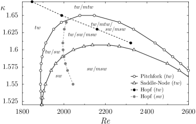
Figure 7: (a) Real (solid) and complex (dashed) relevant eigenvalues of $tw_{2}$ (black) and $sw_{1}$ (gray) along their $\kappa=1.63$-continuation curves. Open and filled circles correspond to pitchfork and Hopf bifurcation points, respectively. (b) Bifurcation curves on $(\mbox{{Re}},\kappa)$-parameter space as explained in the legend. Regions of existence of travelling, spiralling, modulated-travelling and modulated-spiralling waves are labelled $tw$, $sw$, $mtw$ and $msw$, respectively.

A real eigenvalue of $tw_{2}$ (black solid line) undergoes two zero-crossings (open circles) at $\mbox{{Re}}=1951.1$ and $\mbox{{Re}}=2335.2$, corresponding to the creation and destruction of a spiralling-wave ($sw_{1}$) branch. Both pitchfork bifurcations are supercritical and the spiralling waves created have one less unstable direction than the travelling waves they originate from. Inbetween the two pitchfork points, at about $\mbox{{Re}}=2159.8$, a complex pair (black dashed line) crosses the imaginary axis at a Hopf point (black circle), and a branch of modulated travelling waves ($mtw$) appears. The initial modulational frequency of these waves is given by the imaginary part of the eigenvalue at the crossing. Here, $\omega=0.02127\;(4U/D)$, corresponding to a period $T=2\pi/\omega=295.5D/(4U)$. Index theory dictates that, due to the travelling waves stability properties just described, spiralling waves must be stable at the low-Re end and Hopf unstable at the high-Re end.

The complex pair duplicated on the spiralling branch (gray dashed line) takes the lead from its travelling counterpart and undergoes a Hopf bifurcation (gray circle) somewhat earlier in Re, generating a branch of modulated spiralling waves ($msw$). These waves bifurcate at $\mbox{{Re}}=2002.1$ with $\omega=0.02214\;(4U/D)$, corresponding to a period $T=283.8D/(4U)$, slightly shorter than for $mtw$. Both Hopf bifurcations are supercritical and the emerging modulated waves inherit the stability of the original waves.

Identical analyses have been carried out for several other values of $\kappa$ in order to explore the topology of parameter space. Tracks of the bifurcation points from figure 7(a) in the $\kappa$-Re parameter space are shown in figure 7(b). A saddle-node bifurcation curve (solid line with triangles), only present for $\kappa\lesssim 1.607$, delimits a region where no middle-branch travelling waves exist, as described above and illustrated in figure 4. A pitchfork bifurcation curve (solid line with open circles) delimits the region of existence of lower-branch spiralling waves ($sw_{1}$). Middle- and upper-branch spiralling waves can extend beyond this region and actually do so as shown in figure 5. In the region where travelling waves exist, modulated travelling waves that preserve the shift-reflect symmetry appear along a Hopf line (black dashed line with filled circles). As the travelling-waves Hopf-line crosses into the region of existence of spiralling waves another Hopf line (gray dashed line with filled circles), duplicated from the original, but related to the destabilisation of spiralling waves, starts running on their continuation surface. Along this line, modulated spiralling waves are created. All these modulated waves acquire the stability properties of the original waves so that both Hopf lines are supercritical. Since the waves go unstable when Re is increased, the region of existence of modulated waves always lies to the right of their respective bifurcation curves.

Figures 8(a) and 8(b) depict the eigenspectra at $(\mbox{{Re}},\kappa)=(2215,1.63)$ of all four coexisting shift-reflect travelling waves and of all three spiralling waves, respectively.

(a)

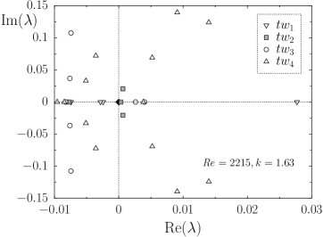
(b)

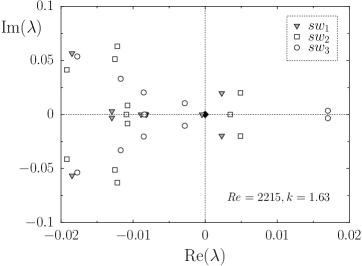
Figure 8: Spectra of (a) travelling and (b) spiralling waves at $(\mbox{{Re}},\kappa)=(2215,1.63)$ as indicated in figure 3(a). Eigenvalues are coded as explained in the legend. The black diamond at the origin represents degenerate eigenmodes corresponding to infinitesimal translation and rotation of the waves.

Apart from the degenerate eigenmodes corresponding to infinitesimal translations and rotations shared by all waves (filled black square at the origin), $tw_{1}$ (downward-pointing triangles in figure 8a) has a single unstable real eigenmode, a relict from the saddle-node at which the wave was created together with $tw_{2}$. The upper-branch wave, $tw_{4}$ (upward-pointing triangles), exhibits, after a long sequence of destabilisations and restabilisations that go beyond the scope of this study, a total of seven unstable directions: an unstable shift-reflect-symmetric complex pair, and an unstable real eigenvalue and two complex pairs pointing out of the symmetry subspace. As shown in figure 7(a), $tw_{2}$ has both an unstable real eigenvalue and an unstable complex pair at $\mbox{{Re}}=2215$. The unstable real eigenmode of $tw_{2}$ (shaded squares) is shift-reflect antisymmetric and points in the direction of $sw_{1}$. Its symmetry-breaking nature is clear from figure 9(a), where mean axial velocity contours are shown to be exactly antisymmetric and axial vorticity has a dominant sign, a feature that is imprinted upon $sw_{1}$. Of course, shooting in the opposite direction (changing the sign of the eigenmode), the shift-reflect-conjugate version of $sw_{1}$ can be found.

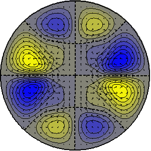
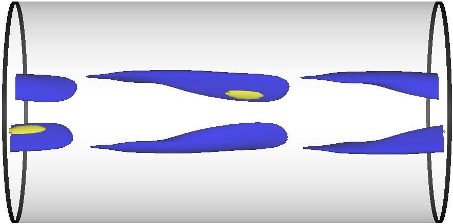
(a)			(b)

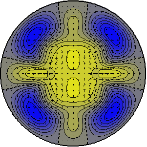
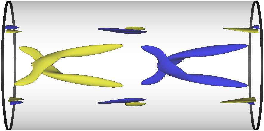
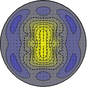
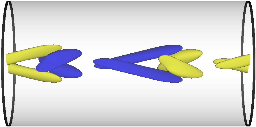
Figure 9: Unstable eigenmodes of $tw_{2}$ (see figure 8a) at $(\kappa,\mbox{{Re}})=(1.63,2215)$. Shown are averaged cross-sectional axial velocity contours with in-plane velocity vectors and three-dimensional isosurfaces of axial vorticity (blue -dark- for negative, yellow -light- for positive). (a) Symmetry-breaking real eigenmode. (b) Real (top) and imaginary (bottom) parts of the symmetry-preserving unstable complex pair. Axial vorticity has been scaled ($\omega_{z}(\mbox{Im})=5\omega_{z}(\mbox{Re})$) to aid visualisation.

The leading complex pair of $tw_{2}$ are shift-reflect symmetric and point in the direction of an invariant unstable manifold leading to a modulated travelling wave that will be described later on. The real and imaginary parts of the eigenmode are shown in figure 9(b), where axial vorticity isosurfaces of the real part are rescaled by a factor of $5$ to make real and imaginary parts of comparable magnitude. The shift-reflect character of the complex pair is clear from the figure. The upper-middle-branch wave $tw_{3}$ (circles) has an unstable shift-reflect-symmetric real eigenvalue (figure 10a), presumably left from the saddle-node at which the wave merges with $tw_{2}$ at higher Re, and an additional symmetry-breaking real eigenvalue inherited from $tw_{2}$. The associated eigenmode is shown in figure 10(b) and preserves some of the features of the unstable symmetry-breaking eigenmode of $tw_{2}$, such as the streaks layout and the signature of the vortical structure, although their respective symmetry-breaking unstable manifolds have deformed and may already lead to different phase space regions.

Spiralling waves $sw_{2}$ (squares in figure 8b) and $sw_{3}$ (circles) exhibit an unstable real eigenvalue together with a complex pair and just a complex pair, respectively. The real unstable eigenvalue of middle-branch $sw_{2}$ is the remnant of saddle-node bifurcations relating the wave with $sw_{1}$ and $sw_{3}$ at other values of Re and $\kappa$. The unstable manifold defined by it is therefore expected to lead to $sw_{1}$ and $sw_{3}$ at either side of $sw_{2}$. The complex pair, shared by all three spiralling waves, is at the origin of a branch of modulated spiralling waves branching off $sw_{1}$ that will be described later. This eigenmode has been represented in figure 10(c).

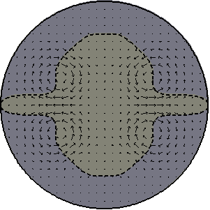
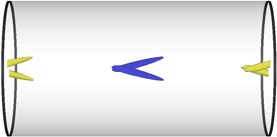
(a)			(c)
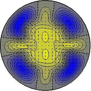
(b)

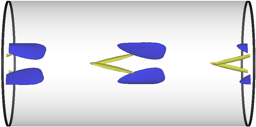
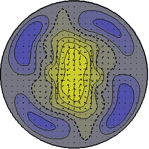
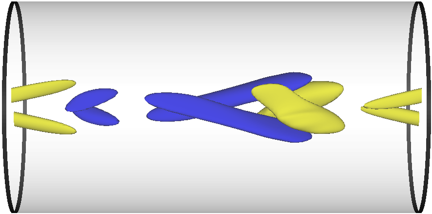
Figure 10: Unstable eigenmodes of $tw_{3}$ (see figure 8a) and $sw_{1}$ (see figure 8b) at $(\kappa,\mbox{{Re}})=(1.63,2215)$. (a) Symmetry-preserving real eigenvector of $tw_{3}$. (b) Symmetry-breaking real eigenvector of $tw_{3}$. (c) Real (top) and imaginary (bottom) parts of the unstable complex pair of $sw_{1}$. Shown are averaged cross-sectional axial velocity contours with in-plane velocity vectors and three-dimensional isosurfaces of axial vorticity (blue -dark- for negative, yellow -light- for positive). Axial vorticity has been scaled ($\omega_{z}(\mbox{Im})=5\omega_{z}(\mbox{Re})$) to aid visualisation.

This complex pair of eigenvectors is remarkably similar to that of $tw_{2}$ (figure 9b). They look alike in all respects except that the latter preserves the shift-reflect symmetry, while the former does not. The fact that both Hopf lines of figure 7(b) coalesce in a single point in $(\kappa,\mbox{{Re}})$ parameter space is not a coincidence. In fact, it is to be expected that modulated travelling waves and modulated spiralling waves are related by a pitchfork bifurcation of a symmetric fixed cycle Kuznetsov (1995).

All unstable eigenmodes of figure 8 have been reported in the last two columns of table 1, either in $ev\in S$ or $ev\in\bar{S}$, depending on whether they do or do not belong to the shift-reflect subspace, respectively.

4 Time-dependent solutions

The Hopf bifurcations prepare the stage for the appearance of time-dependent solutions. Only $2$-fold azimuthally-periodic flows will be considered, so that time-dependent solutions that are stable within this subspace can be computed through symmetry-restricted time evolution. Unless otherwise stated, this is the only symmetry enforced in the numerical representation, while all other symmetries are unconstrained and may be broken.

4.1 Modulated travelling waves

In the symmetry-preserving Hopf bifurcation on the lower-middle travelling-wave branch ($tw_{2}$) a shift-reflect-symmetric time-periodic solution appears which is a modulated travelling wave, also referred to as a relative periodic orbit. As Re is increased, a complex pair of eigenvalues crosses into the unstable half of the complex plane as shown in figure 7(a) for $\kappa=1.63$ and extended for all $\kappa$ in figure 7(b). In the $\kappa$-range of interest, the pitchfork bifurcation occurs before the Hopf bifurcation. As a consequence, modulated waves emerging from the Hopf instability, although supercritical, must be expected to inherit all previous instabilities. Accordingly, at $\kappa=1.63$, emerging modulated travelling waves are pitchfork unstable at onset.

Fortunately, the Hopf instability belongs precisely in the symmetry subspace that the pitchfork instability breaks, so that the latter can be suppressed by restricting time-evolution to the shift-reflect subspace. It is precisely the fact that shift-reflect-restricted time evolution unveils a stable branch of modulated travelling waves pointing towards increasing Re, that indicates that the Hopf bifurcation is supercritical in the sense that the first Lyapunov coefficient is negative Kuznetsov (1995).

Thus, a branch of shift-reflect modulated travelling waves ($mtw$) has been unfolded at $\kappa=1.63$ and represented in figure 3(a) (filled diamonds). The shape of the continuation curve is suggestive of a turning point in a fold-of-cycles at about $\mbox{{Re}}\simeq 2337$, implying the existence of a saddle branch of cycles of larger amplitude. The consequences of this were advanced in figure 1 and will be discussed below. Let us first focus on the nodal branch and analyse one of the solutions.

Figure 11 shows two alternative axial-drift-independent phase map projections of a modulated travelling wave solution at $(\kappa,\mbox{{Re}})=(1.63,2335)$.

(a)

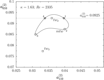
(b)

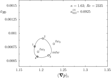
Figure 11: Phase map projections of a modulated travelling wave ($mtw$) at $(\kappa,\mbox{{Re}})=(1.63,2335)$. (a) $a_{010}^{(2)}$ vs $a_{110}^{(2)}$. (b) Three-dimensional energy ($\varepsilon_{\rm 3D}$) vs axial pressure gradient ($(\boldsymbol{\nabla}p)_{z}$). Middle-branch travelling waves ($tw_{2}$ and $tw_{3}$) have been labelled and marked with open squares. Positive and negative crossings of a Poincaré section defined by $a_{010}^{(2)}=a_{010}^{(2)}(tw_{2})$ are indicated by plus signs and crosses, respectively. Numbered circles correspond to snapshots in figure 13.

The solution describes a closed loop and can therefore be seen as a relative periodic orbit. Travelling waves, which are degenerate or relative equilibria, and solutions bifurcating from them have a pure frequency associated to the advection speed (solid-body translation). Time series of local quantities such as point velocities or pressures are necessarily imprinted by this frequency, but the modulation disappears by restating the problem in a comoving frame. Global quantities such as modal energies or volume averaged fields naturally overlook solid-body rotation and translation, making them suitable for a decoupled analysis in the direction orthogonal to the degenerate drift. Thus, as justified before, the bifurcation analysis of travelling waves can be carried out analogously to that of fixed points, as long as special care is taken in the neighbourhood of homoclinic connections Rand (1982); Golubitsky et al. (2000). The Hopf bifurcation adds a modulational frequency to the pure translational frequency. As a result, global quantities cease to be constant and oscillate with this frequency, while the representation of local quantities would have made the solution appear as quasiperiodic.

At $\mbox{{Re}}=2335$, close to the presumed fold-of-cycles, the modulation has grown large around the travelling wave ($tw_{2}$) from which it originally bifurcated. To allow comparison with other solutions that will be discussed later, a Poincaré section at $a_{010}^{(2)}=a_{010}^{(2)}(tw_{2})$ has been defined. The trajectory pierces the Poincaré section twice, so it is convenient to differentiate between positive and negative crossings (plus signs and crosses, respectively, in figure 11). This Poincaré section is special in the sense that it is independent of the degenerate drift. Using global quantities is equivalent to working in a reference frame moving with the wave. In this way, drifting waves drop from the analysis, while modulated waves appear as equilibria of the Poincaré application and doubly-modulated waves (or relative tori) as discrete cycles.

The time dependence is clarified by figure 12(a), where axial phase speed ($c_{z}$, black line) and mean axial pressure gradient ($(\boldsymbol{\nabla}p)_{z}$, gray line) time-series along a full period of the solution have been represented.

(a)

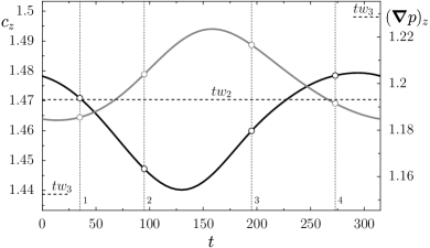
(b)

Figure 12: Modulated travelling wave ($mtw$) at $(\kappa,\mbox{{Re}})=(1.63,2335)$. (a) Axial phase speed ($c_{z}$, black line) and axial pressure gradient ($(\boldsymbol{\nabla}p)_{z}$, gray line) time-series. Dotted horizontal lines indicate the values for $tw_{2}$ and $tw_{3}$ while numbered vertical lines and open circles indicate snapshots in figure 13. (b) Fourier transform of the non-axisymmetric streamwise-dependent modal energy contents ($\varepsilon_{\rm 3D}$). Part of the time signal is plotted in the inset.

Comparing the time signals with the constant value for middle-branch travelling waves ($tw_{2}$ and $tw_{3}$, horizontal dotted lines) it becomes clear that the modulated wave oscillates around $tw_{2}$, and seems to visit $tw_{3}$ once along every period, although figure 11 seems to discard too close a visit. Both signals oscillate $\pm 1\%$ around a mean value that has an offset when compared with $tw_{2}$. On average, the driving pressure gradient is slightly higher and the axial drift rate slower than for the travelling wave. This follows from the fact that we are no longer close to the bifurcation point and nonlinear effects have long kicked in. The Fourier transform of the energy contained in non-axisymmetric streamwise-dependent modes ($\varepsilon_{\rm 3D}$) has been plotted in figure 12(b), with the time signal shown in the inset frame. The spectrum reveals that the solution has a strong mean component and a peak angular frequency at $\omega_{0}=0.0199\;(4U/D)$, corresponding to a period $T_{0}=2\pi/\omega_{0}=315.2D/(4U)$. This period is extremely long when compared with the streamwise advection time-scale, which is of order $2\pi/(\kappa c_{z})\sim 3$. The signal is not strictly sinusoidal and some energy is spread among a number of harmonics of $\omega_{0}$.

To better convey the modulational character of the instability, a few snapshots (conveniently marked in figures 11 and 12a) of the flow field along a cycle have been represented in figure 13 (see online movie).

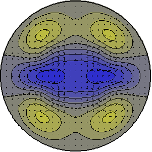
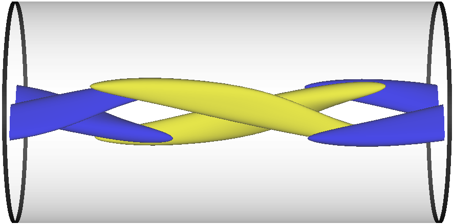
($1$)			($2$)
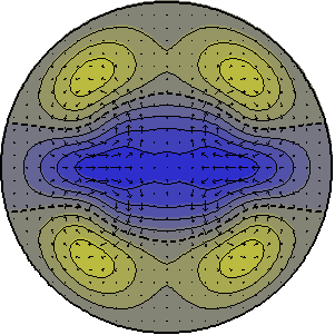
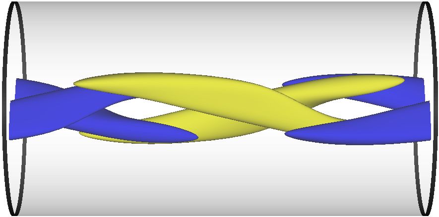
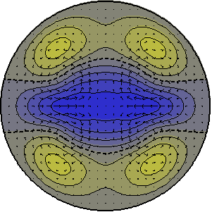
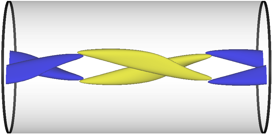
($3$)			($4$)

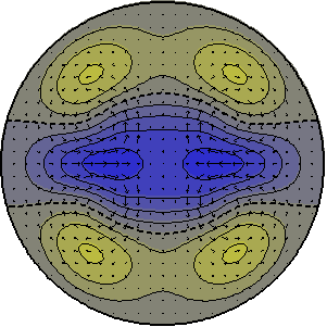
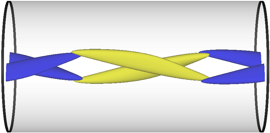
Figure 13: Modulated travelling wave at $(\kappa,\mbox{{Re}})=(1.63,2335)$. Left: $z$-averaged cross-sectional axial velocity contours spaced at intervals of $\Delta\langle u_{z}\rangle_{z}=0.1U$. In-plane velocity vectors are also displayed. Right: axial vorticity isosurfaces at $\omega_{z}=\pm 1U/D$. Fluid flows rightwards. Blue (dark gray) for negative, yellow (light) for positive. ($1$) $t=35$, ($2$) $t=95$, ($3$) $t=195$ and ($4$) $t=273$ $D/(4U)$. To avoid drift due to streamwise advection, snapshots are taken in a comoving frame moving with the instantaneous advection speed from figure 12(a). The snapshots have been indicated with empty circles in figures 11 and 12(a).

It is clear from the snapshots that the modulated wave indeed oscillates around $tw_{2}$ (figure 2b) and that, as noted, preserves the shift-reflect symmetry. As expected from the mild oscillation of all time signals, the modulation is not very prominent and the snapshots look all fairly similar.

4.2 Modulated spiralling waves

The Hopf bifurcation on the branch of spiralling waves occurs at lower Re than on the branch of travelling waves (figure 7b). Spiralling wave $sw_{1}$ loses stability in a supercritical Hopf and a branch of stable modulated spiralling waves emerges, pointing in the direction of increasing Re. Three of such branches have been plotted in figure 3 (filled circles, labelled $msw$) for varying $\kappa$ (shading as explained in the legend).

Figure 14 shows a three-dimensional phase map projection on the space defined by $(a_{010}^{(2)},a_{110}^{(2)},a_{100}^{(2)})$ of a modulated spiralling wave ($msw$) at $(\kappa,\mbox{{Re}})=(1.63,2185)$.

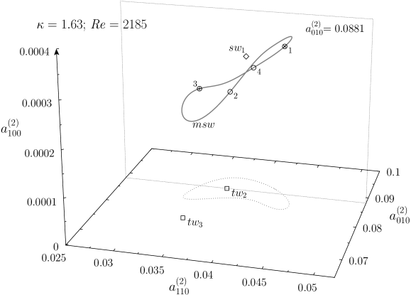
Figure 14: Three-dimensional phase map projection $(a_{010}^{(2)},a_{110}^{(2)},a_{100}^{(2)})$ of a modulated spiralling wave ($msw$) at $(\kappa,\mbox{{Re}})=(1.63,2185)$. Middle-branch travelling waves ($tw_{2}$ and $tw_{3}$) have been labelled and marked with open squares and spiralling wave ($sw_{1}$) with an open diamond. Positive and negative crossings of a Poincaré section defined by $a_{010}^{(2)}=a_{010}^{(2)}(tw_{2})$ are indicated by plus signs and crosses, respectively. Numbered circles correspond to snapshots in figure 17.

The wave describes a closed loop in phase space surrounding the spiralling wave ($sw_{1}$) from which it bifurcated, and it does so at a finite amplitude of $a_{100}^{(2)}$, away from the shift-reflect subspace where this coefficient cancels exactly. The projection on the shift-reflect subspace (light gray dotted line on the $a_{100}^{(2)}=0$ plane) is reminiscent of figure 11(a), even if Re is different, which suggests that both waves are related by a pitchfork of cycles.

A couple of additional phase map projections have been represented in figure 15.

(a)

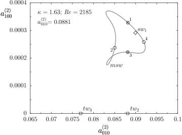
(b)

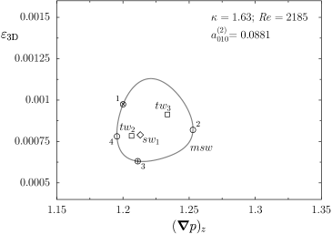
Figure 15: Phase map projections of a modulated spiralling wave ($msw$) at $(\kappa,\mbox{{Re}})=(1.63,2185)$. (a) $a_{100}^{(2)}$ vs $a_{010}^{(2)}$. (b) Three-dimensional energy ($\varepsilon_{\rm 3D}$) vs axial pressure gradient ($(\boldsymbol{\nabla}p)_{z}$). Middle-branch travelling waves ($tw_{2}$ and $tw_{3}$) have been labelled and marked with open squares and spiralling wave ($sw_{1}$) with an open diamond. Positive and negative crossings of a Poincaré section defined by $a_{010}^{(2)}=a_{010}^{(2)}(tw_{2})$ are indicated by plus signs and crosses, respectively. Numbered circles correspond to snapshots in figure 17.

Figure 15(a) shows the projection of figure 14 on the $(a_{100}^{(2)},a_{010}^{(2)})$ plane, while figure 15(b) represents the same trajectory in the $(\varepsilon_{\rm 3D},(\boldsymbol{\nabla}p)_{z})$ plane. Comparison of the latter with figure 11(b) further supports the connection between $msw$ and $mtw$.

The variables used for phase map representation naturally filter the frequencies associated to degenerate drifts. In this case, since we are dealing with a modulated spiralling wave bifurcated from a spiralling wave, not only the axial phase speed ($c_{z}$) is masked, but also the azimuthal rotation rate ($c_{\theta}$). Together with the modulational (Hopf) frequency, two additional frequencies associated to drifts are involved, although only the former is relevant to the dynamics. Both phase speeds have been plotted along a full period of $msw$ in figure 16(a).

(a)

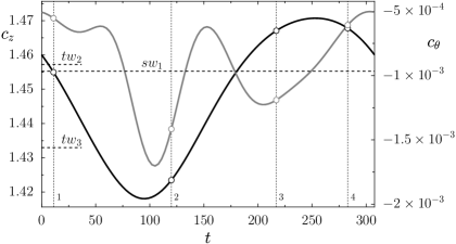
(b)

Figure 16: Modulated spiralling wave ($msw$) at $(\kappa,\mbox{{Re}})=(1.63,2185)$. (a) Axial ($c_{z}$, black line) and azimuthal ($c_{\theta}$, gray line) phase speed time-series. Dotted horizontal lines indicate the values for $sw_{1}$, $tw_{2}$ and $tw_{3}$ while numbered vertical lines and open circles indicate snapshots in figure 17. (b) Fourier transform of the non-axisymmetric streamwise-dependent modal energy contents ($\varepsilon_{\rm 3D}$). Part of the time signal is plotted in the inset.

They oscillate around the spiralling wave values with a certain offset due to nonlinear effects. Figure 16(b) shows the Fourier spectrum of the energy signal in the inset. As was already observed for $mtw$, also $msw$ has a slow modulation angular frequency of $\omega_{0}=0.0204\;(4U/D)$, corresponding to a period $T_{0}=307.8D/(4U)$. The fact that both periods are of the same order reinforces the suspicion that they are a consequence of the same mechanism.

Snapshots corresponding to the time instants indicated with circles in figures 14, 15 and 16(a), have been plotted in figure 17 (see online movie).

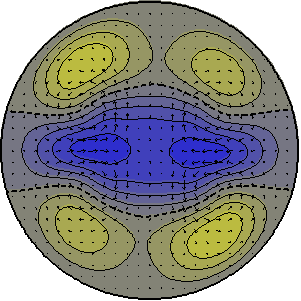
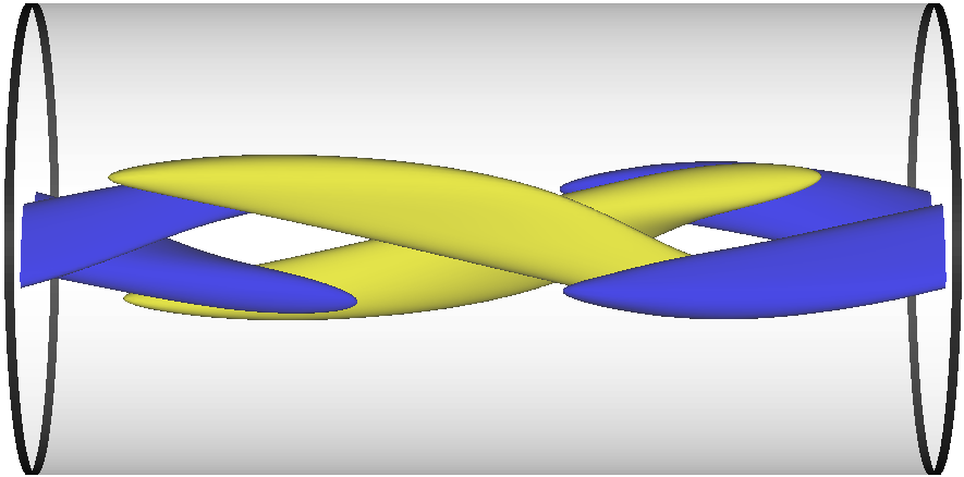
($1$)			($2$)
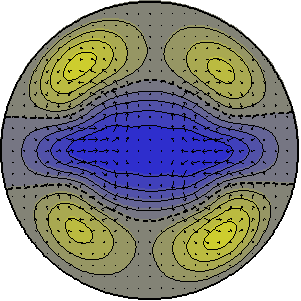
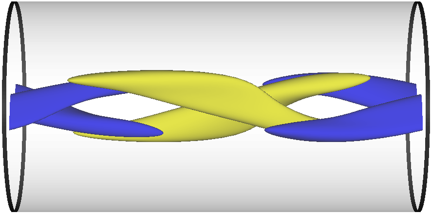
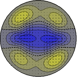
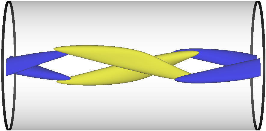
($3$)			($4$)

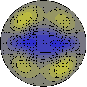
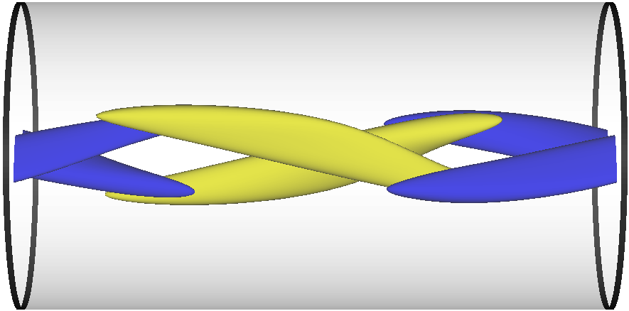
Figure 17: Modulated spiralling wave at $(\kappa,\mbox{{Re}})=(1.63,2185)$. Left: $z$-averaged cross-sectional axial velocity contours spaced at intervals of $\Delta\langle u_{z}\rangle_{z}=0.1U$. In-plane velocity vectors are also displayed. Right: axial vorticity isosurfaces at $\omega_{z}=\pm 1U/D$. Fluid flows rightwards. Blue (dark gray) for negative, yellow (light) for positive. ($1$) $t=11$, ($2$) $t=120$, ($3$) $t=217$ and ($4$) $t=283$ $D/(4U)$. To avoid drift due to streamwise advection, snapshots are taken in a comoving frame spiralling with the instantaneous advection speeds from figure 16(a). The snapshots have been indicated with circles in figures 14, 15 and 16(a).

As was the case for $mtw$ of figure 13, the modulational character of $msw$ is very mild. Nevertheless, it clearly orbits around $sw_{1}$ and the symmetry-breaking is fairly clear at all times.

At the lower $\kappa$ explored (light solid circles in figure 3b), the modulated spiralling waves branch seems to undergo a fold-of-cycles. The bifurcation scenario presented in figure 1 is not applicable to this lower $\kappa$. At higher $\kappa$, instead, modulated waves lose stability to doubly-modulated spiralling waves in a supercritical Neimark-Sacker bifurcation.

4.3 Doubly-modulated spiralling waves

In an appropriately spiralling frame of reference, modulated spiralling waves appear as periodic orbits. A Poincaré section can be defined as in previous section to analyse the stability of the orbit. When considering the Poincaré map associated to the relative periodic orbit, the solution reduces to a simple equilibrium and discrete-time bifurcation analysis can be applied.

For high enough $\kappa$, modulated spiralling waves undergo a supercritical Neimark-Sacker bifurcation (Hopf of cycles) that occurs away from strong resonances Kuznetsov (1995). Bifurcated waves are relative quasiperiodic solutions involving $2$ degenerate and $2$ modulational frequencies, adding up to $4$ frequencies. The two extrema (minimum and maximum) that were used to represent modulated waves split in four to convey the existence of a modulation of the modulation (figure 3, filled circles, labelled $m^{2}sw$). This is visible at the highest Re values for $\kappa=1.60$ (intermediate-gray) and more clearly, yet in a short range of less than $10$ Re-units, for $\kappa=1.63$ (black).

Track of the doubly-modulated waves at $\kappa=1.60$ is lost shortly after they bifurcate in what seems to be a fold-of-tori that will not be pursued here. At this $\kappa$, the bifurcation diagram of figure 1 would be complicated in ways that make it inaccessible. The more extended existence of doubly-modulated waves at $\kappa=1.63$ leaves enough room for them to evolve nonlinearly away from modulated waves so that they can be properly analysed.

Figure 18 shows a three-dimensional phase map projection on the space defined by $(a_{010}^{(2)},a_{110}^{(2)},a_{100}^{(2)})$ of a doubly-modulated spiralling wave ($m^{2}sw$) at $(\kappa,\mbox{{Re}})=(1.63,2205)$.

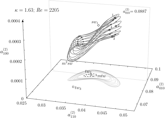
Figure 18: Three-dimensional phase map projection $(a_{010}^{(2)},a_{110}^{(2)},a_{100}^{(2)})$ of a doubly-modulated spiralling wave ($m^{2}sw$) at $(\kappa,\mbox{{Re}})=(1.63,2205)$. Middle-branch travelling waves ($tw_{2}$ and $tw_{3}$) have been labelled and marked with open squares and spiralling wave ($sw_{1}$) with an open diamond. Positive and negative crossings of a Poincaré section defined by $a_{010}^{(2)}=a_{010}^{(2)}(tw_{2})$ are indicated by plus signs and crosses, respectively. Numbered circles correspond to snapshots in figure 21.

The modulated spiralling wave ($msw$) from which $m^{2}sw$ bifurcates has gone unstable and is therefore inaccessible. Nevertheless, it can be safely presumed that it looks similar to $msw$ as shown for $\mbox{{Re}}=2185$ in figure 17 and that it must be contained within the region of phase space delimited by the invariant torus on which $m^{2}sw$ runs. Looking at the Poincaré section, it is easy to identify the drift undergone by the wave after every flight. The drift goes in a circle, appearing as an invariant cycle on the Poincaré map.

Doubly-modulated waves will generally be dense-filling on the torus (quasiperiodic), since no resonant conditions are enforced by any of the symmetries of the problem and the new frequency does not necessarily need to be commensurate with the previously existing modulation frequency inherited from the modulated wave. However, as the parameter is varied, Arnold tongues might be crossed and phase locking occur producing parameter windows where periodic orbits exist. The torus persists under small parameter variations but the orbit structure will be dependent on whether the rotation number of the map defined by Poincaré reduction is rational or irrational. As a matter of fact, the wave shown in figure 18 exhibits a rational proportion between the two frequencies, as can be seen in figure 19.

(a)

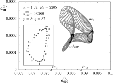
(b)

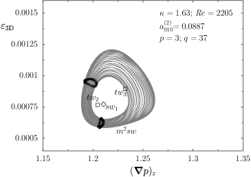
Figure 19: Phase map projections of a doubly-modulated spiralling wave ($m^{2}sw$) at $(\kappa,\mbox{{Re}})=(1.63,2205)$. (a) $a_{100}^{(2)}$ vs $a_{010}^{(2)}$. The inset shows a Poincaré section defined by $a_{110}^{(2)}=a_{110}^{(2)}(tw_{2})$. (b) Three-dimensional energy ($\varepsilon_{\rm 3D}$) vs axial pressure gradient ($(\boldsymbol{\nabla}p)_{z}$). The Poincaré section is defined by $a_{010}^{(2)}=a_{010}^{(2)}(tw_{2})$. Middle-branch travelling waves ($tw_{2}$ and $tw_{3}$) have been labelled and marked with open squares and spiralling wave ($sw_{1}$) with an open diamond. Positive and negative crossings of Poincaré sections are indicated by plus signs and crosses, respectively.

The orbit structure and the Poincaré sections clearly show that the wave is a $(3,37)$-cycle: the cycle makes $37$ revolutions along the modulated wave trajectory (short modulation period) and $3$ around the invariant curve on the Poincaré map (long modulation period) before closing. The $37$th iterate of the Poincaré map is therefore a fixed point. The existence of a stable $(3,37)$-cycle implies that an unstable $(3,37)$-cycle must also exist Kuznetsov (1995). This is the only phase locking identified in this study, meaning that all other doubly-modulated waves found are dense or, at least, of extremely long period.

The Neimark-Sacker modulational frequency is much higher than the inherited Hopf frequency. Phase-speed time-series along a full cycle around the Poincaré section for the wave at $(\kappa,\mbox{{Re}})=(1.63,2205)$ are shown in figure 20(a).

(a)

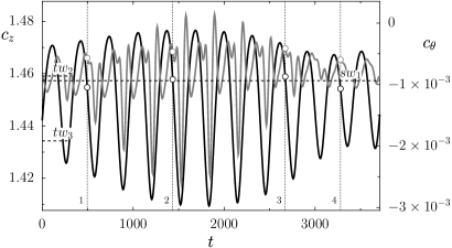
(b)

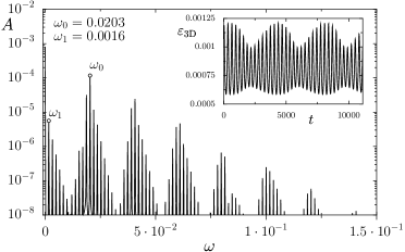
Figure 20: Doubly-modulated spiralling wave ($m^{2}sw$) at $(\kappa,\mbox{{Re}})=(1.63,2205)$. (a) Axial ($c_{z}$, black line) and azimuthal ($c_{\theta}$, gray line) phase speed time-series. Dotted horizontal lines indicate the values for $sw_{1}$, $tw_{2}$ and $tw_{3}$ while numbered vertical lines and open circles indicate snapshots in figure 21. (b) Fourier transform of the non-axisymmetric streamwise-dependent modal energy contents ($\varepsilon_{\rm 3D}$). Part of the time signal is plotted in the inset.

The signal is of about the same frequency as that in figure 16(a), but now, it is slightly modulated with a much longer period. The spectrum of the energy signal shown in figure 20(b) features the same peaks, corresponding to the fast modulation $\omega_{0}=0.0203$, as that of the modulated wave (figure 16b), except that additional peaks at multiples of the slow frequency $\omega_{1}=0.001649$ appear in the scene. The spectrum is still discrete, as should be expected from a quasiperiodic signal, but now two frequencies are identifiable. In this case, due to phase locking, the ratio of frequencies is rational and coincides precisely with the rotation number ($\rho=\omega_{1}/\omega_{0}=p/q=3/37$).

The slow period is very long ($T_{1}=2\pi/\omega_{1}\simeq 3810.3D/(4U)$), which makes it difficult to select just a few snapshots that are representative of the time dependence of the wave. Nevertheless, the modulation along the short period has already been exemplified for a modulated spiralling wave in figure 17 and should be fairly similar for a bifurcated doubly-modulated wave. Therefore, we will focus here on the slow modulation effect by representing the drift experienced by the wave every time the Poincaré section is pierced. Figure 21 (see online movie) shows four such crossings of the Poincaré section defined by $a_{010}^{(2)}=a_{010}^{(2)}(tw_{2})$ as indicated in figure 18.

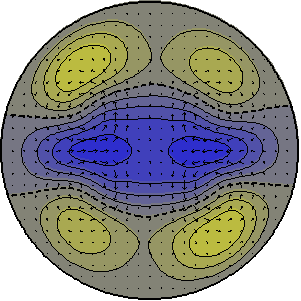
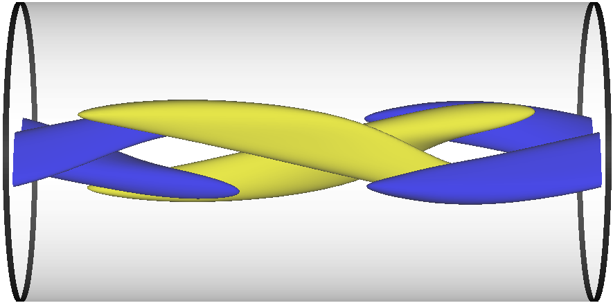
($1$)			($2$)
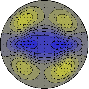
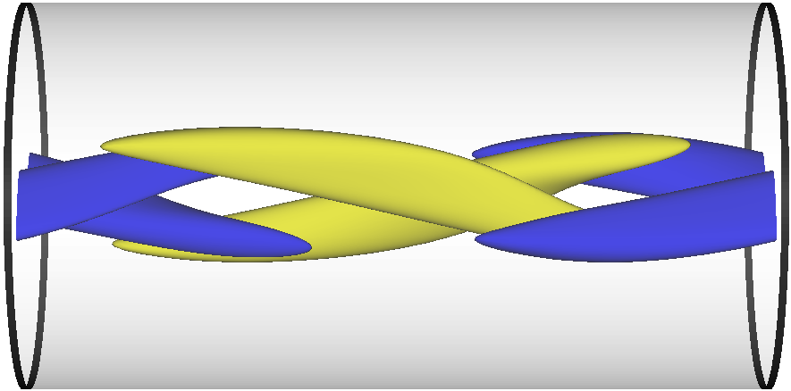
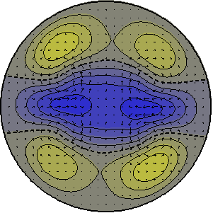
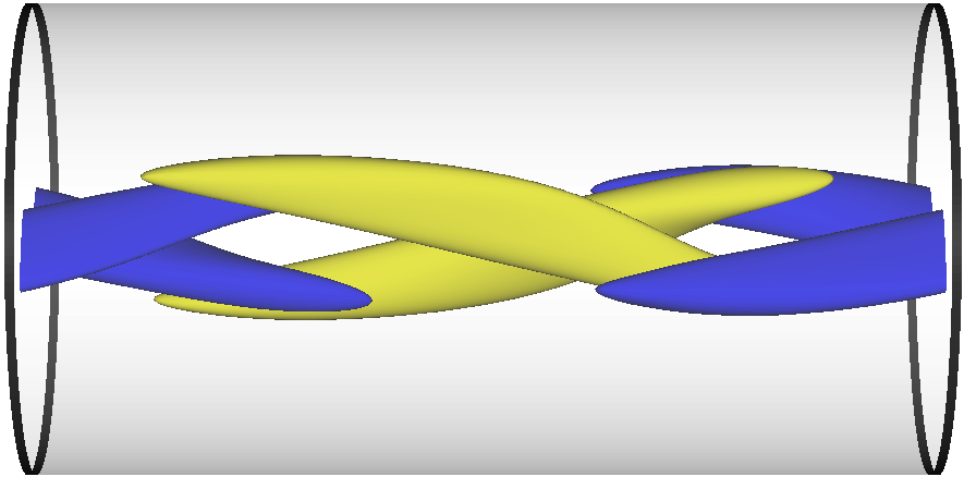
($3$)			($4$)

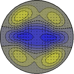
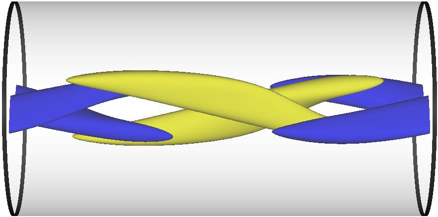
Figure 21: Doubly-modulated spiralling wave at $(\kappa,\mbox{{Re}})=(1.63,2205)$. Left: $z$-averaged cross-sectional axial velocity contours spaced at intervals of $\Delta\langle u_{z}\rangle_{z}=0.1U$. In-plane velocity vectors are also displayed. Right: axial vorticity isosurfaces at $\omega_{z}=\pm 1U/D$. Fluid flows rightwards. Blue (dark gray) for negative, yellow (light) for positive. ($1$) $t=495$, ($2$) $t=1435$, ($3$) $t=2672$ and ($4$) $t=3280$ $D/(4U)$. To avoid drift due to streamwise advection, snapshots are taken in a comoving frame spiralling with the instantaneous advection speeds from figure 20(a). The snapshots have been indicated with circles in figures 18 and 20(a).

The solution, which originally bifurcated at zero amplitude with respect to the modulated spiralling wave, has barely left the linear regime. Consequently, the modulation is extremely mild and only a close inspection reveals that there is any modulation at all. The four snapshots should be compared with figure 17($1$) and seen as a modulation of it, since it represents the unique point at which $msw$ crosses the Poincaré section.

Increasing Re at $\kappa=1.63$ results in a significant swell of the invariant torus and an ulterior catastrophic transition into a chaotic attractor.

4.4 Mildly chaotic spiralling waves

Doubly-modulated travelling waves cease to exist abruptly and the new dynamics are organised along pseudoperiodic trajectories. These solutions largely preserve some of the features of the original torus at some stages but depart frantically at some other stages. Reattachment to the remnants of the torus never occurs at the same point, introducing a mild degree of chaoticity.

A full pseudo-period of a time-evolving chaotic spiralling wave ($cw$) at $(\kappa,\mbox{{Re}})=(1.63,2215)$ has been represented in figure 22.

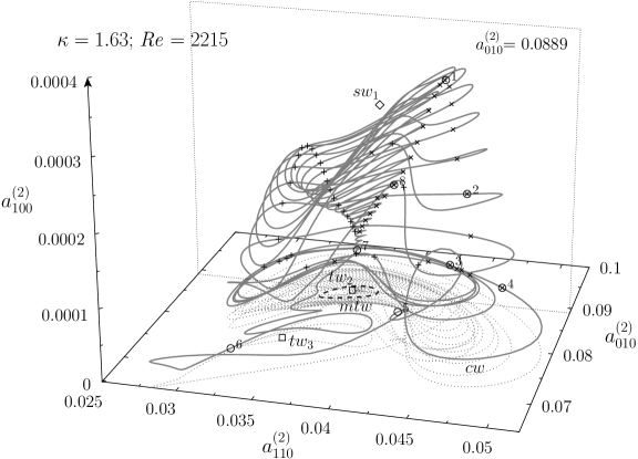
Figure 22: Three-dimensional phase map projection $(a_{010}^{(2)},a_{110}^{(2)},a_{100}^{(2)})$ of a chaotic spiralling wave ($cw$) at $(\kappa,\mbox{{Re}})=(1.63,2215)$ along a full pseudo-period. Middle-branch travelling waves ($tw_{2}$ and $tw_{3}$) have been labelled and marked with open squares and spiralling wave ($sw_{1}$) with an open diamond. A coexisting modulated travelling wave ($mtw$, black dashed line) has also been represented. Positive and negative crossings of a Poincaré section defined by $a_{010}^{(2)}=a_{010}^{(2)}(tw_{2})$ are indicated by plus signs and crosses, respectively. Numbered circles correspond to snapshots in figure 25.

For a while, the orbit runs on the remnants of the invariant torus that existed at lower Re (figure 18). As it goes around, though, the flow is unable to close as before, and the trajectory is thrown away and gets hooked in a seemingly periodic motion as if it was captured by the stable manifold of some periodic orbit. All this happens at very low $a_{100}^{(2)}$, which is indicative of a close approach to the shift-reflect subspace. After some turns, the trajectory departs again with a violent thrust and then reconnects back onto what seems to be the unstable manifold of $tw_{2}$. Finally, following this manifold, the trajectory makes its trip back onto the torus-dominated region and the process starts anew.

Several pseudo-periods of the wave have been represented in a couple of phase map projections (figure 23) to illustrate its mildly chaotic character.

(a)

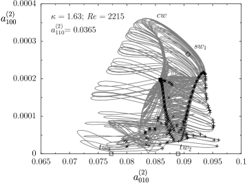
(b)

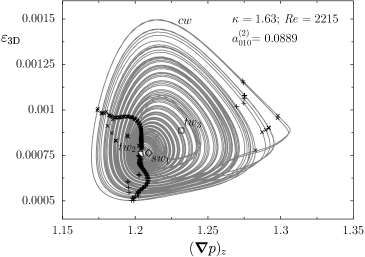
Figure 23: Phase map projections of a chaotic spiralling wave ($cw$) at $(\kappa,\mbox{{Re}})=(1.63,2215)$ along several pseudo-periods. (a) $a_{100}^{(2)}$ vs $a_{010}^{(2)}$. Marks indicate crossings of a Poincaré section defined by $a_{110}^{(2)}=a_{110}^{(2)}(tw_{2})$. (b) Three-dimensional energy ($\varepsilon_{\rm 3D}$) vs axial pressure gradient ($(\boldsymbol{\nabla}p)_{z}$). The Poincaré section is defined by $a_{010}^{(2)}=a_{010}^{(2)}(tw_{2})$. Middle-branch travelling waves ($tw_{2}$ and $tw_{3}$) have been labelled and marked with open squares and spiralling wave ($sw_{1}$) with an open diamond. Positive and negative crossings of Poincaré sections are indicated by plus signs and crosses, respectively.

The Poincaré map in figure 23(a) tends to be dense and deterministic at the upper tip, where the solution runs on the torus (to be compared with figure 19a). Meanwhile, the lower side features a chaotic cloud of random crossings. Furthermore, the return funnel that gets the trajectory back on the torus exhibits a variable width that can get as narrow as in figure 22. The $\varepsilon_{\rm 3D}$ vs $(\boldsymbol{\nabla}p)_{z}$ phase map also gives a clear view on the fate of the torus. While at $\mbox{{Re}}=2205$ (figure 19b) the doughnut shape with closed $mtw$-centred orbits on the Poincaré sections was clearly identifiable, at $\mbox{{Re}}=2215$ (figure 23b), the hole has been disrupted and long excursions to high three-dimensional energy values and large axial pressure gradients occur.

Time signals preserve the fast frequency associated to the old Hopf instability, while the slow frequency resulting from the Neimark-Sacker instability is exchanged for a longer period modulation that is no longer constant. Phase speed time-series for a pseudo-period of the chaotic wave at $(\kappa,\mbox{{Re}})=(1.63,2215)$ have been drawn in figure 24(a).

(a)

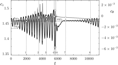
(b)

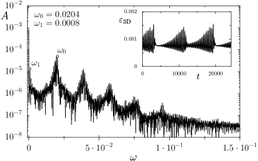
Figure 24: Chaotic spiralling wave ($cw$) at $(\kappa,\mbox{{Re}})=(1.63,2215)$. (a) Axial ($c_{z}$, black line) and azimuthal ($c_{\theta}$, gray line) phase speed time-series. Dotted horizontal lines indicate the values for $sw_{1}$, $tw_{2}$ and $tw_{3}$ while numbered vertical lines and open circles indicate snapshots in figure 25. (b) Fourier transform of the non-axisymmetric streamwise-dependent modal energy contents ($\varepsilon_{\rm 3D}$). Part of the time signal is plotted in the inset.

Both signals undergo a steady amplitude growth before becoming somewhat chaotic. Phase speed modulations get fairly large just before the chaotic transient, with the azimuthal phase speed ($c_{\theta}$) even changing sign, which means that at some intervals the wave becomes retrograde. Towards the end of the chaotic transient, the azimuthal phase speed vanishes as the wave approaches the shift-reflect subspace and, shortly after, the axial phase speed ($c_{z}$) evolves towards lower-middle-branch travelling-wave values ($tw_{2}$). From there on, the wave evolves as if it was following the combined pitchfork-Hopf-unstable manifold of $tw_{2}$ and the process restarts. It is remarkable how, despite the close visit to the shift-reflect subspace, and even if the azimuthal speed changes sign, the wave always makes its way back to the same side of phase space. There are no reversals, contrary to what happens for the Lorenz attractor Strogatz (1994), and the shift-reflect-conjugate side of phase space is never visited. Therefore, a shift-reflect-symmetric chaotic attractor spiralling with opposite rotation rate exists and the two attractors do not interact.

The inset of figure 24(b) illustrates the variable nature of the long modulational period. The spectral energy density of the signal reflects this variability. There still are clear peaks at the high frequency $\omega_{0}=0.0204\;(4U/D)$ and its harmonics, largely preserved from modulated and doubly-modulated spiralling waves. The long period modulation, though, is no longer represented by a discrete peak, but by a certain dispersion around $\omega_{1}\simeq 0.0008\;(4U/D)$. The pseudo-period is much longer than for doubly-modulated waves due to the fact that the wave spends large amounts of time in a region of phase space not visited by $m^{2}sw$. The effect of the dispersion is that the wave ceases to be quasiperiodic and the spectrum becomes continuous.

To portray the time-dependence of the flow field, several snapshots of the chaotic spiralling wave along a pseudo-period have been gathered in figure 25.

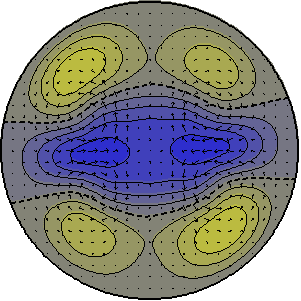
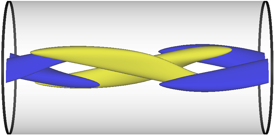
($1$)			($2$)
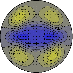
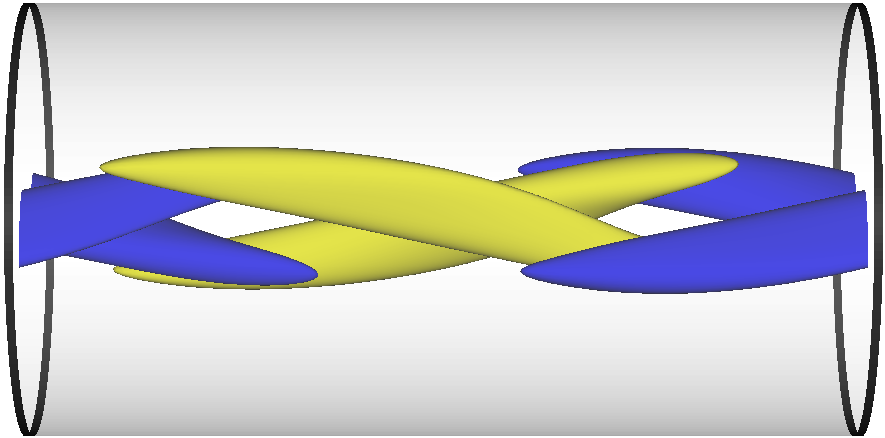
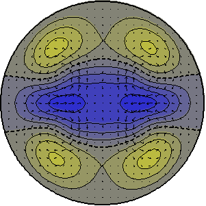
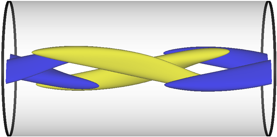
($3$)			($4$)
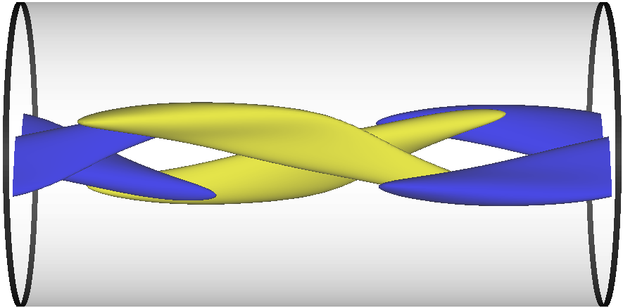
($5$)			($6$)
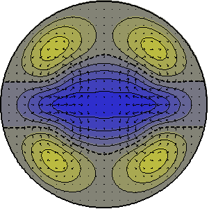
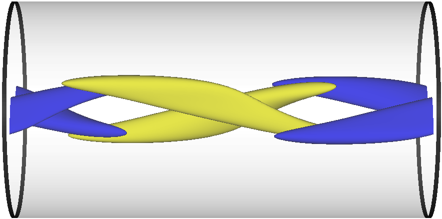
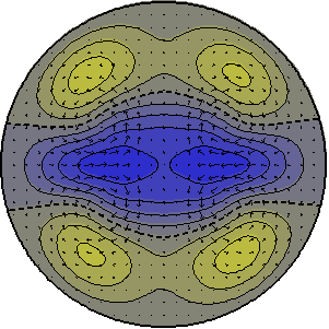
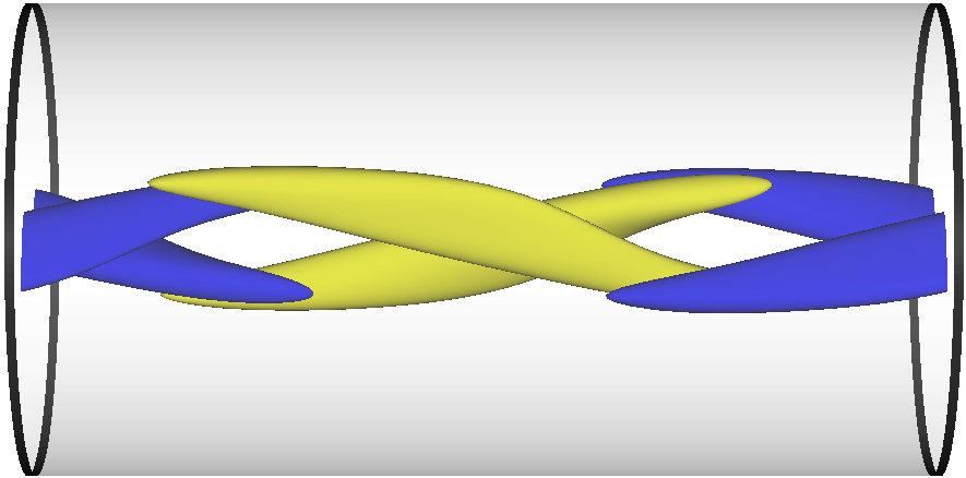
($7$)			($8$)

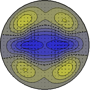
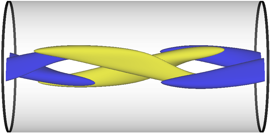
Figure 25: Chaotic spiralling wave at $(\kappa,\mbox{{Re}})=(1.63,2215)$. Left: $z$-averaged cross-sectional axial velocity contours spaced at intervals of $\Delta\langle u_{z}\rangle_{z}=0.1U$. In-plane velocity vectors are also displayed. Right: axial vorticity isosurfaces at $\omega_{z}=\pm 1U/D$. Fluid flows rightwards. Blue (dark gray) for negative, yellow (light) for positive. ($1$) $t=1974$, ($2$) $t=3569$, ($3$) $t=4547$, ($4$) $t=5526$ , ($5$) $t=5654$ , ($6$) $t=5771$ , ($7$) $t=7000$ and ($8$) $t=10196$ $D/(4U)$. To avoid drift due to streamwise advection, snapshots are taken in a comoving frame spiralling with the instantaneous advection speeds from figure 24(a). The snapshots have been indicated with circles in figures 22 and 24(a).

To reduce the number of snapshots to a minimum and at the same time allow comparison with $m^{2}sw$, flow fields have been represented either on the same Poincaré section as in figure 21 (snapshots $1$-$4$ and $8$) or along the violent escape in the vicinity of the shift-reflect subspace (snapshots $5$-$7$).

Snapshots ($1$), ($2$) and ($8$) clearly correspond to time-instants at which the trajectory runs on the torus. It is not surprising that they look similar to the corresponding snapshots ($1$, $2$ and $4$ in figure 21) of $m^{2}sw$. Snapshots ($3$) and ($4$), notwithstanding the fact that they correspond to Poincaré crossings, exemplify new dynamics. They are in a region of phase space away from where the torus existed and very close to the shift-reflect subspace, as is apparent from the clearly identifiable quasi-symmetry planes of the cross-sections. Snapshot ($3$) belongs in the region where $cw$ seems to get hooked on a periodic orbit, while snapshot ($4$), taken at the time the violent excursion starts, seems to confirm it, as it holds great similarity with ($3$). The axial pressure gradient peak in figure 23(b) is represented by snapshot ($5$), where the streaks are clearly very strong and the shift-reflect symmetry fairly clear. Snapshot ($6$) shows the closest visit to the shift-reflect subspace and is, at the same time, a disputably close visit to $tw_{3}$ (figure 2c) as indicated by both cross-sectional axial velocity contours and axial-vorticity isosurfaces. ($4$)-($6$) occurs in a small fraction of the full trajectory, which ultimately justifies the description of the escape as violent. The shift-reflect symmetry starts to be disrupted again in snapshot ($7$) and the wave evolves slowly as if departing away from $tw_{2}$ along its unstable pitchfork-Hopf manifold. The flow field in ($7$) is clearly half way between $tw_{2}$ (figure 2b) and $sw_{1}$ (figure 6a). At ($8$) the symmetry has been completely broken and the flow field reattaches to the remnants of the invariant torus.

4.5 Phase-locked wave

As in many systems (see, e.g. logistic map, Strogatz, 1994) where a chaotic attractor develops, there exist parameter intervals where the solution locks onto a stable periodic orbit. These are called periodic windows, and the chaotic set described above is no exception.

At $\mbox{{Re}}=2209.7$, very slightly above torus breakdown and creation of the chaotic set, and for a tiny interval, the flow becomes periodic. The periodic trajectory, which looks very similar to the pseudoperiodic trajectory at $\mbox{{Re}}=2215$, has been represented in figure 26.

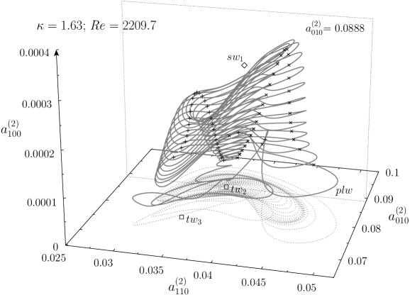
Figure 26: Three-dimensional phase map projection $(a_{010}^{(2)},a_{110}^{(2)},a_{100}^{(2)})$ of a phase-locked spiralling wave ($plw$) at $(\kappa,\mbox{{Re}})=(1.63,2209.7)$ along a full period. Middle-branch travelling waves ($tw_{2}$ and $tw_{3}$) have been labelled and marked with open squares and spiralling wave ($sw_{1}$) with an open diamond. Positive and negative crossings of a Poincaré section defined by $a_{010}^{(2)}=a_{010}^{(2)}(tw_{2})$ are indicated by plus signs and crosses, respectively.

Phase speeds have been plotted in figure 27(a) for comparison with $cw$.

(a)

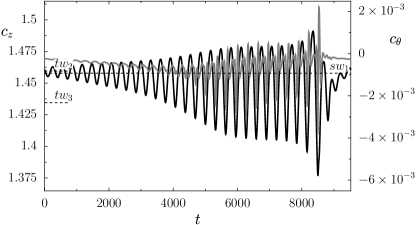
(b)

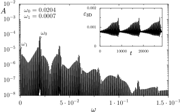
Figure 27: Phase-locked spiralling wave ($plw$) at $(\kappa,\mbox{{Re}})=(1.63,2209.7)$. (a) Axial ($c_{z}$, black line) and azimuthal ($c_{\theta}$, gray line) phase speed time-series. Dotted horizontal lines indicate the values for $sw_{1}$, $tw_{2}$ and $tw_{3}$. (b) Fourier transform of the non-axisymmetric streamwise-dependent modal energy contents ($\varepsilon_{\rm 3D}$). Part of the time signal is plotted in the inset.

Chaos disappears but the invariant torus is not reestablished and the shift-reflect escape is preserved. The slowly evolving interval that we identified as an approach to the unstable manifold of $tw_{2}$ is no longer as clear, and the return funnel is wide from the beginning, so that amplitude modulation is present all along. Despite the close resemblance of all time-signals to some of the pseudo-periods at $\mbox{{Re}}=2215$, time-stamps are now strictly periodic and the Fourier transform of three-dimensional energy time-series is again discrete as was the case at $\mbox{{Re}}=2205$. The fast frequency $\omega_{0}=0.0204\;(4U/D)$ is clearly identifiable with the Hopf instability, while the slow frequency $\omega_{1}=0.0006596\;(4U/D)$ is inherited from $cw$ but now takes a sharp value and fits exactly an integer number of times in $\omega_{0}$.

We do not provide snapshots of the flow structures at selected times along a period because of the close resemblance they bear with those shown for $\mbox{{Re}}=2215$ in figure 25.

4.6 Turbulent transients

At somewhat larger Re the chaotic set ceases to be an attractor and cannot hold trajectories indefinitely. Figure 28 exemplifies two departures from the chaotic set at $\kappa=1.63$ and $\mbox{{Re}}=2235$ and $2240$.

(a)

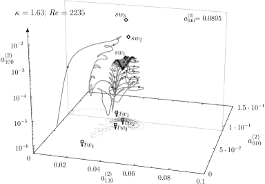
(b)

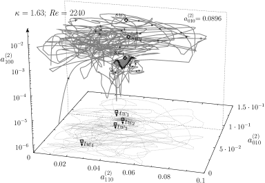
Figure 28: Three-dimensional phase map projection $(a_{010}^{(2)},a_{110}^{(2)},a_{100}^{(2)})$ of two escapes from the chaotic set. (a) $(\kappa,\mbox{{Re}})=(1.63,2235)$. (b) $(\kappa,\mbox{{Re}})=(1.63,2240)$. Travelling waves ($tw_{1}$, $tw_{2}$, $tw_{3}$ and $tw_{4}$) have been labelled and marked with open squares and spiralling waves ($sw_{1}$, $sw_{2}$ and $sw_{3}$) with open diamonds. Positive and negative crossings of a Poincaré section defined by $a_{010}^{(2)}=a_{010}^{(2)}(tw_{2})$ are indicated by plus signs and crosses, respectively.

Logarithmic scale has been used for the vertical axis to aid visualisation. The dense structure in the middle of the figure is the remains of the chaotic attractor, which preserves the same structure as for lower Re, except that it is no longer an attractor. For both Re shown, the solution departs in pretty much the same direction towards the region in phase space where the strongly spiralling waves $sw_{2}$ and $sw_{3}$ are. At $\mbox{{Re}}=2235$ (figure 28a), the trajectory does not reach the waves and relaminarisation follows shortly. Instead, at $\mbox{{Re}}=2240$ (figure 28b), the flow reaches the location where spiralling waves live and is kicked towards turbulence. The solution stays turbulent for around $1000D/(4U)$ and finally relaminarises, oddly enough, along a path that seems close to that followed at $\mbox{{Re}}=2235$.

Full understanding of the actual nature of the $2$-fold azimuthally-symmetric turbulent saddle is beyond the scope of this study and the issue will not be pursued further. It is nevertheless pertinent to stress that turbulence does occur within the azimuthal subspace and even when computations are further restricted to preserve the shift-reflect symmetry.

5 Formation and destruction of the chaotic attractor

Most of the transitions between states reported in this study, once the drifts due to axial and azimuthal degeneracy have been appropriately tackled, are of a local nature and conspicuously well understood. This is not the case of the transition from doubly-modulated waves to mildly chaotic waves. There are several known paths whereby deterministic solutions revolving around an invariant torus become chaotic when the torus disappears. Some of them have been described in the context of turbulent transition. Landau (1944) suggested quasiperiodic motion resulting from an infinite cascade of bifurcating incommensurable frequencies that ultimately lead to turbulence. Ruelle & Takens (1971) and Newhouse, Ruelle & Takens (1978) modified the scenario to include dissipative systems, such as viscous fluids, that do not, in general, have quasiperiodic motions. Their route to chaos involved successive bifurcations from a stable equilibrium into a stable limit cycle followed by transition to a stable $2$-torus and then to chaos. The scenario, though, does not give a full description of all possible bifurcation scenarios leading to the destruction of a $2$-torus and does not provide conditions under which chaos may or may not follow. Some scenarios have been analysed by generalising Floquet theory in systems without symmetry Chenciner & Iooss (1979) and some theorems on torus breakdown have been formulated Anischenko, Safonova & Chua (1993). These theorems, known under the name Afraimovich-Shilnikov theorems, suggest three distinct scenarios: (i) breakdown due to some ordinary bifurcation of phase-locked limit cycles such as period doubling (flip) or Neimark-Sacker; (ii) sudden transition to chaos due to the appearance of a homoclinic connection; (iii) breakdown following from a gradual loss of smoothness. We will argue that our one-dimensional path follows (ii).

Very valuable information can be retrieved from the frequency of quasiperiodic solutions as they approach the bifurcation point. As shown in figure 29(a), the fast angular frequency ($\omega_{0}$) evolves smoothly through the Neimark-Sacker bifurcation from modulated to doubly-modulated waves. So much so, that the bifurcation point for $\kappa=1.63$ (black solid line) at $\mbox{{Re}}\sim 2199$ is not discernible and doubly-modulated waves inherit this Hopf frequency directly from modulated waves.

(a)

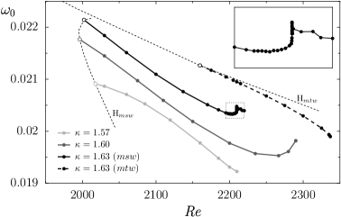
(b)

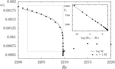
Figure 29: (a) Fast angular frequency ($\omega_{0}$) of all time-dependent solutions as a function of Re and $\kappa$. Solid lines for spiralling waves and dashed for travelling. Shading for varying $\kappa$ as indicated in the legend. Hopf bifurcation curves are indicated with dotted lines and labelled (H_mtw and H_msw). The inset shows a close-up of the small dotted square. (b) Slow frequency ($\omega_{1}$) of doubly-modulated waves at $\kappa=1.63$. The dotted-square-region is zoomed-in in the inset with a coordinate transformation ($T_{1}=2\pi/\omega_{1}$ vs $\log(\mbox{{Re}}_{c}-\mbox{{Re}})$).

As quasiperiodic motion evolves, the frequency grows slightly but remains bounded and stabilises at a fairly constant value (on average) for chaotic waves after the global bifurcation has taken place. In contrast, the slow frequency ($\omega_{1}$) experiences substantial variation across the bifurcation, as is evident from figure 29(b). Since the two frequencies associated to degenerate drifts ($c_{z}$ and $c_{\theta}$) are constant and $\omega_{0}$ is nearly constant, while the period $T_{1}=2\pi/\omega_{1}$ becomes unbounded, we will represent the $4$-torus as a limit cycle and relative limit cycles as equilibria. We can do this because constant and nearly constant frequencies do not play a role in the dynamics near bifurcation points.

Infinite-period bifurcations are commonly associated with homoclinic or heteroclinic behaviour. The two most typical cases are the saddle-node and the saddle-loop homoclinic bifurcations, depending on whether the bifurcating orbit becomes homoclinic to a non-hyperbolic or to an hyperbolic equilibrium, respectively Strogatz (1994); Kuznetsov (1995). One of the mensurable properties that allows to discriminate between the two is the way in which the period diverges. When a saddle-node develops on a limit cycle, the period diverges according to:

$$T_{1}=\frac{2\pi}{\omega_{1}}\sim\frac{C}{\sqrt{\mbox{{Re}}_{c}-\mbox{{Re}}}}+D,$$ (15)

where $\mbox{{Re}}_{c}$ is the critical Re, and $C$ and $D$ are fitting parameters. Meanwhile, when a cycle grows to collide with a hyperbolic saddle and then disappear in a saddle-loop bifurcation, the period diverges logarithmically, like Gaspard (1990)

$$T_{1}=\frac{2\pi}{\omega_{1}}\sim-\lambda^{-1}\log(\mbox{{Re}}_{c}-\mbox{{Re}})+D,$$ (16)

where the factor $\lambda$ is the eigenvalue of the unstable direction of the hyperbolic fixed point and $\log$ represents the natural logarithm.

The behaviour of the period near a saddle-loop bifurcation may be extended to more complex scenarios such as Shilnikov bifurcations in n-dimensional dynamical systems or even tori collision with hyperbolic limit cycles Marques, Lopez & Shen (2001), while the saddle-node homoclinic trend is also observed in the case of orbits homoclinic to nonhyperbolic equilibria or to other nonhyperbolic cycles (e.g. a blue sky catastrophe, see Meca, Mercader, Batiste & Ramírez-Piscina, 2004, but also in the case when the invariant set forms a torus).

The frequency-range of the doubly-modulated-waves is in very good agreement with a logarithmic fit (16) (gray solid line in figure 29b, see the inset). As a result from the fit, an estimated value of $\mbox{{Re}}_{c}=2209.67253$ is obtained for the critical bifurcation point and $\lambda=1.959\times 10^{-3}(4U/D)$. This suggests that the torus might be becoming homoclinic to a hyperbolic saddle cycle with an unstable multiplier of $\mu=\mathrm{e}^{\lambda T_{0}}\simeq 1.8253$ ($T_{0}=307.2D/(4U)$ is the fast period of trajectories on the torus, which should coincide, in the limit, with the period of the saddle cycle) as the bifurcation is approached.

The evolution of the frequency suggests an approach to a homoclinic or, as we will see, a heteroclinic cyclic connection involving hyperbolic orbits. To elucidate with which solution or solutions the torus collides, figure 30 depicts trajectories corresponding to refined approaches to the transition point from either side of the bifurcation.

(a)

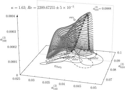
(b)

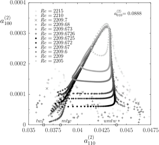
Figure 30: (a) Three-dimensional phase map projection $(a_{010}^{(2)},a_{110}^{(2)},a_{100}^{(2)})$ just before (gray, circles for Poincaré crossings) and after (black, plus signs) transition. (b) Poincaré section showing solutions before (filled circles) and after (plus signs and crosses for phase-locked wave) transition. Travelling waves ($tw_{2}$ and $tw_{3}$) have been labelled and marked with open squares and spiralling wave ($sw_{1}$) with an open diamond. The shift-reflect stable ($mtw$) and unstable ($umtw$) modulated waves (dashed and dashdotted lines in a, open circles in b) are also shown.

Figure 30(a) shows a three-dimensional phase map representation of the stable solution just before (doubly-modulated wave, gray solid line) and after (mildly chaotic wave, black solid line) transition. For a large fraction of the time, both solutions run together, as is clear from the upper part of the plot. However, as the solutions spiral down the outer side of the torus and approach the shift-reflect subspace, the doubly-modulated wave closes on the torus from below, while the chaotic wave is kicked away and frenzies in the vicinity of the shift-reflect subspace for a while before joining the torus back at the inner side to spiral up. The divergence of the trajectories is further evidenced when comparing the crossings on the Poincaré section (open circles for the quasiperiodic wave, plus signs for the chaotic wave). The Poincaré map associated to the doubly-modulated wave describes a triangle-shaped cycle, while the chaotic wave only preserves the upper part of the triangle and breaks down at the lower side. The solutions, as shown in the figure, only revolve once around the torus, but they fill the trajectories on the Poincaré map densely when followed for sufficiently long times.

Figure 30(b) shows these solutions on the Poincaré section, together with an array of solutions at varying distance from either side of the bifurcation point. As transition is approached from $\mbox{{Re}}<\mbox{{Re}}_{c}$ (filled circles getting darker), the cycle gets more and more triangle-shaped, starting from the phase-locked pseudo-circular shape at $\mbox{{Re}}=2205$. The cycles run clockwise. The upper corner remains fixed, while the lower side gets aligned with the shift-reflect subspace, represented by the horizontal axis, and approaches it in a blow-up fashion (note that solutions are not Re-equispaced). For each quasiperiodic wave, a fairly equidistant chaotic wave at the other side of the transition point has been represented (plus signs, crosses for the phase-locked wave at $\mbox{{Re}}=2209.7$). The right side of the chaotic wave closes on the right side of the quasiperiodic wave like a zipper as bifurcation is approached. After departing from the right vertex of the triangle, chaos follows and reattachment to the left side of the torus is less neat.

The trend followed by the right vertex of the triangle suggests that a shift-reflect saddle cycle (a fixed point of the Poincaré map) might be approached. Less clear, due to the chaotic dynamics, but still plausible, is the conjecture that the left vertex approaches the modulated travelling wave ($mtw$). This modulated travelling wave, a stable node in its shift-reflect subspace, was presumed to undergo a fold-of-cycles at around $\mbox{{Re}}\simeq 2337$, thus pairing with a shift-reflect saddle cycle of larger amplitude. This would be the saddle cycle approached by the right vertex. If collision of the torus with the two limit cycles occurred simultaneously, as suggested by figure 30(b) and supported by the fold-pitchfork bifurcation scenario for maps (see Kuznetsov, Meijer & Van Veen, 2004, for the closely related fold-flip bifurcation), a non-robust heteroclinic cycle would be created at $\mbox{{Re}}_{c}$ leaving no attractors. No full description of the fold-pitchfork bifurcation for maps is available in the literature. It would correspond to the analysis of a 1:1 resonance Kuznetsov (1995) in the presence of $Z_{2}$ symmetry and the details are too intricate to be discussed here and shall be treated elsewhere.

Using shift-reflect symmetry-restricted time-evolution and edge-tracking refinement Skufca et al. (2006); Schneider et al. (2007), where the laminar and turbulent asymptotic states have been replaced by two clearly distinct paths towards the stable modulated wave, we have numerically computed the conjectured unstable modulated wave ($umtw$) with sufficient accuracy. It has a single real multiplier outside of the unit circle corresponding to a shift-reflect eigenmode. Its location is perfectly congruent with a collision with the outer surface of the torus (right vertex) as the global bifurcation point is approached (see figure 30).

It can be shown that the $mtw$ branch effectively experiences a fold-of-cycles (a shift-reflect real multiplier crosses the unit circle) and that $umtw$ belongs precisely to the saddle branch created at the fold as schematically shown in figure 1.

Figure 31 shows two alternative axial-drift-independent phase map projections of the unstable modulated travelling wave solution at $(\kappa,\mbox{{Re}})=(1.63,2209.67)$, close to the bifurcation point.

(a)

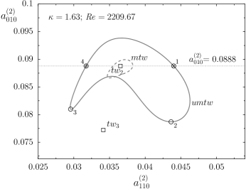
(b)

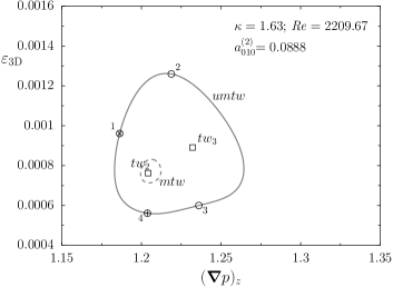
Figure 31: Phase map projections of an unstable modulated travelling wave ($umtw$) at $(\kappa,\mbox{{Re}})=(1.63,2209.67)$. (a) $a_{010}^{(2)}$ vs $a_{110}^{(2)}$. (b) Three-dimensional energy ($\varepsilon_{\rm 3D}$) vs axial pressure gradient ($(\boldsymbol{\nabla}p)_{z}$). Middle-branch travelling waves ($tw_{2}$ and $tw_{3}$) have been labelled and marked with open squares. The modulated travelling wave $mtw$ at the same parameter values is indicated with a dashed line. Positive and negative crossings of a Poincaré section defined by $a_{010}^{(2)}=a_{010}^{(2)}(tw_{2})$ are indicated by plus signs and crosses, respectively. Numbered circles correspond to snapshots in figure 33.

It is a straightforward observation to identify $mtw$ and $umtw$ as bounding solutions for the asymptotic shift-reflect projection of the doubly-modulated wave $m^{2}sw$ as it approaches the bifurcation point (compare the three solutions in figure 30). Especially $umtw$, since $mtw$ seems to be affected by manifold tangles. This correspondence gets even clearer when comparing figure 31(b) and figure 19(b). The projection of the doubly-modulated wave seems to grow in the region bounded by $mtw$ at the inside and $umtw$ at the outside, the heteroclinic bifurcation corresponding to the simultaneous collision with both modulated waves.

The time evolution of $umtw$ is characterised in figure 32(a) through the representation of the axial phase speed ($c_{z}$, black line) and the mean axial pressure gradient ($(\boldsymbol{\nabla}p)_{z}$, gray line) time-series along a full period of the solution.

(a)

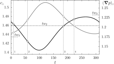
(b)

Figure 32: Unstable modulated travelling wave ($umtw$) at $(\kappa,\mbox{{Re}})=(1.63,2209.67)$. (a) Axial phase speed ($c_{z}$, black line) and axial pressure gradient ($(\boldsymbol{\nabla}p)_{z}$, gray line) time-series. Dotted horizontal lines indicate the values for $tw_{2}$ and $tw_{3}$ while numbered vertical lines and open circles indicate snapshots in figure 33. (b) Fourier transform of the non-axisymmetric streamwise-dependent modal energy contents ($\varepsilon_{\rm 3D}$). Part of the time signal is plotted in the inset.

Comparing the time signals with those for $mtw$ in figure 12(a) it becomes relatively clear that $umtw$ results from an amplification of $mtw$ once it has gone unstable at the fold. The Fourier transform of the energy contained in non-axisymmetric streamwise-dependent modes ($\varepsilon_{\rm 3D}$) has been plotted in figure 32(b), with the time signal shown in the inset frame. The resolution of the spectrum is not as good as for stable waves due to the difficulty in stabilising an unstable wave for sufficiently long times. Nevertheless, the wave can be claimed as sufficiently well converged and it exhibits a clear peak of angular frequency at $\omega_{0}=0.0202\;(4U/D)$, corresponding to a period $T_{0}=2\pi/\omega_{0}=311.2D/(4U)$. The $mtw$ at the same parameter values, has a slightly faster frequency $\omega_{0}=0.0209\;(4U/D)$, amounting to a shorter period $T_{0}=2\pi/\omega_{0}=299.9D/(4U)$.

To better support the relevance of the wave in the dynamics of the problem, a few snapshots (indicated in figures 31 and 32a with circles) of the flow field along a cycle have been represented in figure 33 (see online movie).

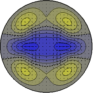
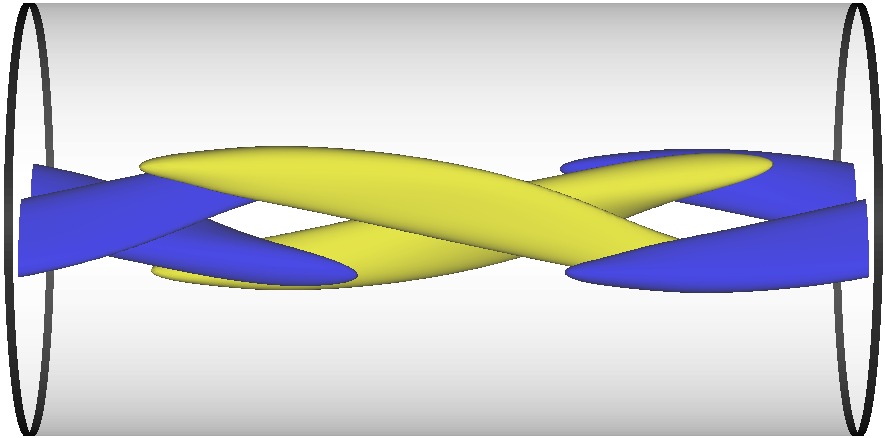
($1$)			($2$)
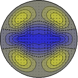
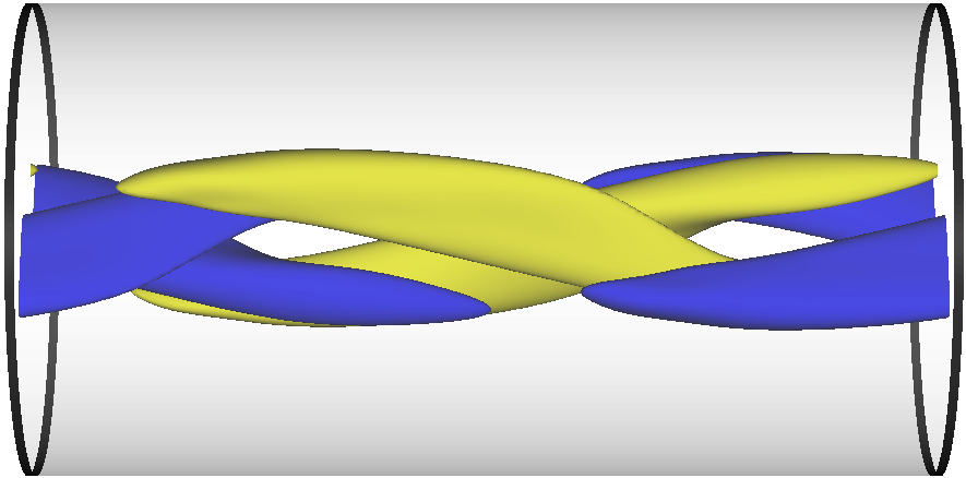
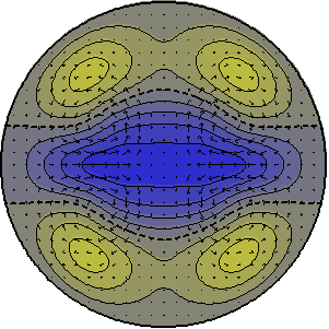
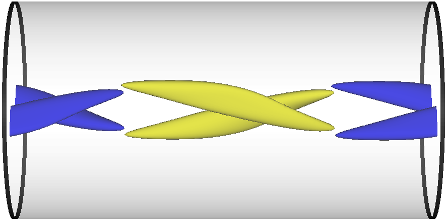
($3$)			($4$)

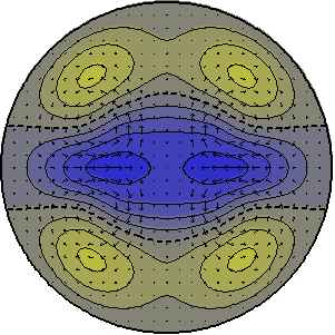
Figure 33: Unstable modulated travelling wave at $(\kappa,\mbox{{Re}})=(1.63,2209.67)$. Left: $z$-averaged cross-sectional axial velocity contours spaced at intervals of $\Delta\langle u_{z}\rangle_{z}=0.1U$. In-plane velocity vectors are also displayed. Right: axial vorticity isosurfaces at $\omega_{z}=\pm 1U/D$. Fluid flows rightwards. Blue (dark gray) for negative, yellow (light) for positive. ($1$) $t=8$, ($2$) $t=58$, ($3$) $t=185$ and ($4$) $t=223$ $D/(4U)$. To avoid drift due to streamwise advection, snapshots are taken in a comoving frame moving with the instantaneous advection speed from figure 32(a). The snapshots have been indicated with empty circles in figures 31 and 32(a).

It is clear from the snapshots that the modulation is similar but of slightly larger amplitude than that for $mtw$ at $\mbox{{Re}}=2335$ (figure 13). Significantly relevant is also the resemblance born by snapshot ($1$) to that of figure 25($3$) corresponding to an approach to the shift-reflect space of the chaotic wave $cw$ at $\mbox{{Re}}=2215$. This fact, added to the similarities of the phase map trajectories (see the winding of the trajectory near the shift-reflect subspace in figure 22) clearly underlines the influence of this wave on the dynamics even at Re-values beyond the global bifurcation.

The bifurcation scenario introduced in figure 1 is now schematically developed in figure 34(a-d).

(a)		(b)	(c)	(d)
		$\overbrace{\textrm{\makebox[286.19078pt][c]{}}}$
		(e)	(f)	(g)

Figure 34: Schematic phase map representation on a Poincaré section of the formation and destruction of the chaotic set. (a), (b), (c) and (d) represent an approximating interpolated flow. (e), (f) and (g) sketch the heteroclinic tangencies expected instead of (c). Phase maps are symmetric with respect to the horizontal axis, which represents the shift-reflect subspace, but only the upper half is shown.

A stable modulated spiralling wave (filled circle) and two saddle modulated travelling waves (open circles on the horizontal axis, which represents the shift-reflect subspace) exist for sufficiently low Re (figure 34a). Strictly speaking, phase maps are symmetric with respect to the horizontal axis and a symmetry-related stable modulated spiralling wave should have been drawn. For simplicity, though, only the upper half is actually represented. In figure 34(b), the modulated spiralling wave has undergone a Neimark-Sacker bifurcation and a stable doubly-modulated wave has been created (thick solid loop). This wave grows and collides with both modulated travelling waves simultaneously in figure 34(c), generating an heteroclinic cycle that leaves this phase-space region open in figure 34(d), as observed for $\mbox{{Re}}\gtrsim 2225$.

The phase maps sketched correspond to approximating the Poincaré application by an interpolating flow. For the real map, heteroclinic cycles ($hc$ in figure 1) will not generically arise. Instead, heteroclinic tangles and tangencies will typically occur, broadening the bifurcation point (or curve) into a wedge where complex dynamics and chaos are common feature. This is precisely what was observed in §4. The appearance of chaotic waves, and the transition point here discussed, would then be related to the first heteroclinic tangency of the stable and unstable modulated waves manifolds (figure 34e). Chaotic waves exist for a finite range of the parameter (figure 34f) but end up disappearing and causing the phase space region they inhabited to open up (figure 34g), so that the flow can leave towards other regions. In the present case towards turbulent motion, as described above.

In the Re-range where chaotic waves exist, the manifolds entanglement and interweaving is complicated by the presence of the travelling- and spiralling-wave solutions discussed in §3. It is not possible with the tools at hand to gain a complete understanding of what the role of relative equilibria and their manifolds is in organising the dynamics around the chaotic set. An example of the complex interminglement of manifolds is visible in figure 30(b) for $\mbox{{Re}}=2209.6726$, where the reattachment to the remnants of the torus is sometimes accomplished along the unstable manifold of the travelling wave $tw_{2}$ rather than along that of the modulated travelling wave $mtw$ as is clear from the alignment of black plus signs.

All things considered, the torus breakdown scenario involving a homoclinic or, rather, heteroclinic-cyclic connection, seems to be the most plausible. The logarithmic fit of the period is supportive of this surmise, except that the fitting parameter $\lambda$ needs to be reinterpreted and it is not clear as to which of either modulated waves it is related. The unstable multiplier associated to $mtw$ has been measured and its value $\mu_{mtw}=1.1265$ corresponds to an eigenvalue $\lambda=3.972\times 10^{-4}(4U/D)$, which is one order of magnitude smaller than the one resulting from the logarithmic fit. It could well be that the unstable manifold of the saddle cycle takes the lead as the unstable manifold of $mtw$ loses strength in the presence of twisting and tangency. An indicator that this could be happening is the deformation of the bottom left corner of the cycle in figure 30(b), which seems to be adapting to the foldings of the tangle. Unfortunately, the unstable multiplier of $umtw$ cannot by itself explain the divergence of the period, either. Its value $\mu_{umtw}=3.9549$, tantamounts to an eigenvalue $\lambda=4.419\times 10^{-3}(4U/D)$, which is larger, by a factor of two, than the parameter $\lambda$ ajusted by the fit.

6 Conclusion

We have studied the fate of upper-branch travelling waves of a shift-reflect-symmetric family that belongs in the $2$-fold azimuthally-periodic subspace of pipe Poiseuille flow. The special stability properties of these waves, which are stable to perturbations within their azimuthal subspace in some regions of parameter space, assist bare time-evolution into converging time-dependent solutions that result from ulterior destabilisation of the waves.

Despite the contorted continuation surfaces of these waves when analysed as a function of both axial wavenumber ($\kappa$) and Reynolds number (Re), a one-dimensional path at $\kappa=1.63$ and varying Re suffices to unveil a multitude of increasingly complex solutions that are reported for the first time in pipe flow. Successive transitions to spiralling waves, modulated travelling waves, modulated spiralling waves and doubly-modulated travelling waves have been reported along the way, and the arising solutions described to some extent, in order to exemplify the extreme richness and complexity of the problem, even within a given subspace. The bifurcation cascade has been shown to culminate in a torus breakdown, presumably following a cyclic heteroclinic connection of the stable and unstable manifolds of modulated travelling waves. The usual manifolds entanglement and heteroclinic tangencies that occur in sufficiently high-dimensional (three or more) dynamical systems, gives the simplest explanation to the observed phenomenology, i.e. the formation of an attracting chaotic set upon torus-breakdown and its subsequent dismantlement at higher Re.

The rupture of the chaotic set does no longer support the existence of mildly chaotic waves, and the flow leaves to other regions of phase space, namely $2$-fold azimuthally-symmetric turbulence. Turbulence within the subspace is, as for full-space pipe, sustained transiently by a chaotic saddle that already exists at lower Re and occupies a region of phase space far away from where all solutions here reported lie (except possibly $tw_{4}$, $sw_{2}$ and $sw_{3}$). In this sense, it can be safely asserted that the chaotic set here described plays no significant role in the development of the phase space structures that integrate the turbulent saddle. This is clearly supported by figure 35, where friction factor ($\nu$) is plotted as a function of Re.

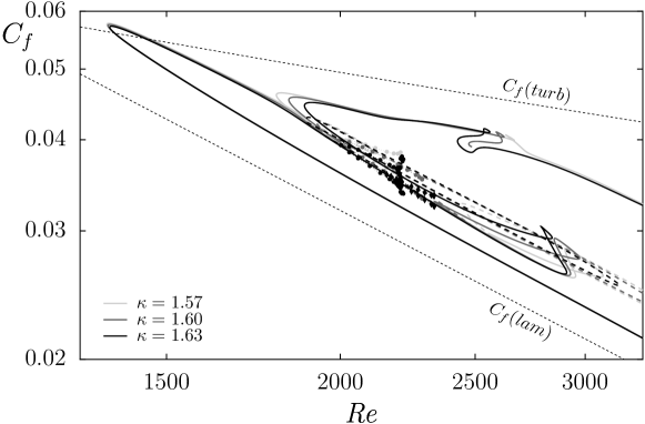
Figure 35: Friction factor ($C_{f}$) as a function of Re and $\kappa$ (shading as explained in the legend). Solid lines represent shift-reflect travelling waves, dashed for spiralling waves. Extrema of time-dependent travelling/spiralling solutions are marked as filled diamonds/circles. Turbulent ($C_{f}(turb)$, from the experimentally obtained log-law $1/\sqrt{C_{f}}=2\log_{10}(\mbox{{Re}}\sqrt{C_{f}})-0.8$; see Schlichting & Gersten, 2000, page 551) and laminar ($C_{f}(lam)=64/\mbox{{Re}}$) friction factor are indicated with dotted lines.

Laminar and turbulent typical friction factor values are indicated with dotted lines to guide the eye. It is evident that, while lower-branch waves approach laminar values and upper-branch waves are close to turbulent friction factors, all other solutions reported in the present study are confined in a narrow stripe halfway between laminarity and turbulence.

It is nevertheless plausible that similar bifurcation cascades might take place in other subspaces for which available simulation tools are currently incapable of overcoming the effects of higher-dimensional unstable manifolds. Some of the chaotic sets thus generated could well go into the formation of a turbulent saddle, although global bifurcations involving several subspaces simultaneously may well complicate the picture even further.

Extending the current analysis to varying $\kappa$ could help better understand the global bifurcation leading to chaos. In particular, continuing time-dependent solutions to larger $\kappa$, preferably along unstable branches where possible, would help clarify the connections among modulated travelling and spiralling waves and, possibly, completely unfold the fold-pitchfork bifurcation of maps here advanced to account for the appearance of chaotic waves.

Also the direct study of $2$-fold azimuthally-symmetric turbulence, which in itself entrains great complexity, may yield results that can help get an intuition as to what may be going on in fully-fledged turbulence. The $2$-fold azimuthally-symmetric subspace has already proven to be a particularly accessible terrain in this respect.