A supercircle description of universal three-body states in two dimensions

Abstract

Bound states of asymmetric three-body systems confined to two dimensions are currently unknown. In the universal regime, two energy ratios and two mass ratios provide complete knowledge of the three-body energy measured in units of one two-body energy. We compute the three-body energy for general systems using numerical momentum-space techniques. The lowest number of stable bound states is produced when one mass is larger than two similar masses. We focus on selected asymmetric systems of interest in cold atom physics. The scaled three-body energy and the two scaled two-body energies are related through an equation for a supercircle whose radius increases almost linearly with three-body energy. The exponents exhibit an increasing behavior with three-body energy. The mass dependence is highly non-trivial. Based on our numerical findings, we give a simple relation that predicts the universal three-body energy.

I Introduction.

The spatial dimensions are crucial for the behavior of quantum systems. The reason for this can be understood by considering the kinetic energy only, and observing that it behaves vastly different in two dimensions as compared to one and three. In fact, the presence of a negative centrifugal barrier for zero angular momentum in two dimensions implies that an infinitesimal attractive potential produces a universal bound state landau ; vol11 . This interesting non-trivial role of the spatial dimensionality can be isolated and studied in detail in the so-called universal limit where the effect of interactions can be described by one or two model-independent quantities and the detailed structure of two-body potentials at short-range thus becomes irrelevant.

The implementation of Feshbach resonances in cold atomic gases chin2010 allows experimenters to tune their systems into the universal regime and study properties that are independent of the particularities of the atoms and molecules. One of the great successes of this program is the observation of three-body Efimov states kraemer2006 ; ferlaino2010 which had been proposed but never found in nuclear physics jen04 . The presence of resonances also allows the study of the strongly correlated unitary limit, where the physics is universal and governed by a single so-called contact parameter tan2008 that is measurable stewart2010 ; kuhnle2010 . Currently there is an experimental push to reduce the ultracold systems from three to two dimensions and study the universal behavior turlapov2010 ; frohlich2011 ; dyke2011 . The highly desired theoretical knowledge of strongly correlated gases is more sparse than in the three-dimensional case. Recently, the contact has been derived using different approaches combescot2009 ; castin2010 ; valiente2011 ; braaten2011 . The question of few-body states in equal mass two-dimensional systems has been addressed in a number of works. Bound states of three- tjo75 ; adh88 ; nie97 ; nie01 ; brod2006 ; kart2006 , four- platter2004 ; brod2006 , and larger particle number droplets hammer2004 ; blume2005 ; lee2006 , and scattering brod2006 and recombination observables helfrich2011 have been addressed.

The general three-body bound state spectrum in the universal limit in two dimensions has not previously been investigated. The limiting case of three identical bosons is known to have exactly one two-body and two three-body bound states in the universal limit tjo75 ; adh88 ; nie97 ; nie01 , and all ratios of energies and radii are universal constants. This is in marked contrast to three dimensions where the Efimov effect produces an infinite ladder of states when the scattering length diverges efi70 . While the results in three dimensions can be obtained through analytical means, the spectrum in the two-dimensional case has been obtained through numerical methods only, and no analytical insights have been found so far. Furthermore, the problem of three particles with different masses and short-range interactions in two dimensions has not been addressed before. The combination of three different species of atoms was recently reported wu2011 . Although that experiment is presently in three dimensions, it should be easily extended to a two-dimensional setup.

The universal limit can be considered in a natural way through zero-range interactions that leave only a single parameter in the potential to be related to the scattering length or two-body bound state energy. Here we numerically solve the momentum-space integral equations in two dimensions bel11 . In three dimensions similar formalism has been discussed within the language of effective field theory braaten2006 . We extract universal features of completely asymmetric three-body systems and provide simple parametrizations of energies as functions of the two-body properties in terms of Lamé curves lame1818 . This provides a uniform parametrization of all aspects of the three-body bound state spectrum in two dimensions that can aid the search for a (semi-)analytical understanding of these intruiging systems.

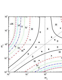
Figure 1: Phase diagram of the maximum number of three-body bound states as functions of two mass ratios, $m_{\alpha}$ and $m_{\beta}$. The three two-body energies are equal, $E_{ab}=E_{bc}=E_{ac}$. The roman numerals indicated the maximum number of bound states in each region. The circular (⁶Li⁴⁰K⁸⁷Rb) and diamond (⁴⁰K⁸⁷Rb¹³³Cs) points are the realistic cases studied in Figs. 3 and 4. The two sets of points are related by the symmetries in Eq. (2).

II Procedure and definitions.

We consider three particles, $a$, $b$, and $c$ of mass $m_{a}$, $m_{b}$, and $m_{c}$ with pairwise contact interactions which produce two-body bound states of energies $E_{ab}$, $E_{ac}$, and $E_{bc}$. The wave equation in momentum space is a set of three coupled integro-differential equations tjo75 ; bel11 ; bel+11 . Here we provide a full survey of the three-body energies, $E_{3}$, in the most general setup. Initially $E_{3}$ is a function of six parameters. However, the use of two-body energies instead of interaction strengths implies that only mass and energy ratios enter the equations. This means that $\epsilon_{3}=E_{3}/E_{ab}$ divided by one of the two-body energies can be expressed as a function of four dimensionless parameters, i.e.

$$\epsilon_{3}=F_{n}\left(\frac{E_{bc}}{E_{ab}},\frac{E_{ac}}{E_{ab}},\frac{m_{b}}{m_{a}},\frac{m_{c}}{m_{a}}\right)\equiv F_{n}(\epsilon_{bc},\epsilon_{ac},m_{\alpha},m_{\beta}),$$ (1)

where $\epsilon_{3}$ is the scaled three-body energy, $m_{\alpha}=m_{b}/m_{a}$, $m_{\beta}=m_{c}/m_{a}$, $\epsilon_{bc}=E_{bc}/E_{ab}$, and $\epsilon_{ac}=E_{ac}/E_{ab}$. The universal functions, $F_{n}$, are labeled by the subscript $n$ to distinguish between ground, $n=0$, and excited states, $n>0$. By interchange of particle labels we find that all the universal functions, $F_{n}$, must obey the symmetry relations:

$$F_{n}\left(\epsilon_{bc},\epsilon_{ac},m_{\alpha},m_{\beta}\right)=F_{n}\left(\epsilon_{ac},\epsilon_{bc},m_{\beta},m_{\alpha}\right)=$$ (2)

$$\epsilon_{bc}F_{n}\left(\frac{1}{\epsilon_{bc}},\frac{\epsilon_{ac}}{\epsilon_{bc}},\frac{1}{m_{\alpha}},\frac{m_{\beta}}{m_{\alpha}}\right)=\epsilon_{bc}F_{n}\left(\frac{\epsilon_{ac}}{\epsilon_{bc}},\frac{1}{\epsilon_{bc}},\frac{m_{\beta}}{m_{\alpha}},\frac{1}{m_{\alpha}}\right)=$$

$$\epsilon_{ac}F_{n}\left(\frac{1}{\epsilon_{ac}},\frac{\epsilon_{bc}}{\epsilon_{ac}},\frac{1}{m_{\beta}},\frac{m_{\alpha}}{m_{\beta}}\right)=\epsilon_{ac}F_{n}\left(\frac{\epsilon_{bc}}{\epsilon_{ac}},\frac{1}{\epsilon_{ac}},\frac{m_{\alpha}}{m_{\beta}},\frac{1}{m_{\beta}}\right).$$

The energy and mass scaling leaves us with four non-trivial parameters. Using the symmetry relations in Eq. (2) we can restrict the investigations of $F_{n}$ to smaller regions of this four-parameter space as indicated by the dashed symmetry lines in Fig. 1.

III Survey of mass dependence.

The mass dependence of the number of three-body bound states for a system with $E_{ab}=E_{ac}=E_{bc}$ is shown. In the central region around equal masses we have the two bound states tjo75 . This region, labeled II, extends in three directions corresponding to one heavy and two rather similar light particles, that is either $m_{\alpha}\sim 1$, $m_{\beta}\sim 1$, or $m_{\alpha}\simeq m_{\beta}\leq 1$. Moving away from these regions in Fig. 1, the number of stable bound states increases in all directions. As an example, consider $m_{\alpha}=10$ and vary $m_{\beta}$ from small to large value in Fig. 1. Perhaps surprisingly, along this line the number of bound states decreases to a minimum of two and subsequently increases again. The reason is that the disappearing states merge into the two-body continuum. The same behavior is found in three dimensions for the disappearance of the infinitely many Efimov states when the attractive strength is increased yam02 . Variation of the two-body energies from all being equal leads to distortion of the figure but the main structure remains. The central region still has the smallest number of stable bound states. Any variation in the two-body energies make region II bigger, pushing the other lines away from the center. Thus, Fig. 1 shows the maximum number of stable bound states for one system described by ($m_{\alpha}$, $m_{\beta}$).

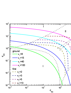
Figure 2: Contour diagrams with lines of fixed $\epsilon_{3}$ values as function of the two-body energies $\epsilon_{ac}$ and $\epsilon_{bc}$. The solid and dashed curves are for ground and excited states, respectively. Here $a$ is ⁸⁷Rb, $b$ is ⁴⁰K, and $c$ is ⁶Li. The dotted curves show where the number of stable bound states change from one (regions most asymmetric for small energies), to two (comparable size of the two-body energies), and to three (equal and large energies). The roman labels I, II, and III are as in Fig. 1.

III.1 Three-body energies for given masses.

Realistic scenarios correspond to given particles (atoms or molecules) with known masses. In contrast, the interactions are variable through Feshbach resonances chin2010 . We therefore assume masses corresponding to alkali atoms ⁸⁷Rb, ⁴⁰K, and ⁶Li. The two ratios of two-body energies are left as variables where each set uniquely specifies the three-body energies of ground and possibly excited states. In Fig. 2, we show a contour diagram of the scaled three-body energies for the two lowest stable bound states. The log-log plot is very convenient for visibility but can be deceiving. On a linear scale the curves of equal scaled three-body energy would look different. However, the parametrizations considered below nonetheless employ the linear scale. The chosen set of masses only allow one, two, or three stable bound states, depending on the two-body energies. The corresponding regions are shown by dotted curves in Fig. 2. The true extent of the regions cannot be seen. Both region II and III are closed, e.g region II continues along region III up to energy ratios of about $10^{\pm 5}$, and the narrow region III is entirely embedded in region II. Other sets of mass ratios could open region III and allow regions inside with more than three stable bound states.

In the log-log plot of Fig. 2 we can see the two-body energies varying by five orders of magnitude, whereas the scaled three-body energies for a stable system must be larger than all two-body energies, and in particular larger than unity since it is measured in units of $E_{ab}$. The three-body energy contours connect minimum and maximum two-body energies, that is zero and maximum two-body energies for the ground state and thresholds boundaries for existence of the excited states. The contours appear in regular intervals with larger values for increasing two-body energies. Large three-body energies reflect small spatial extension and therefore are less interesting as it presumably is unreachable in the universal limit. The contours pass continuously through the boundaries of the different regions since the ground state exists without knowledge of the excited states. The contours in Fig. 2 for the excited state can only appear in the regions with two or more stable bound states. These contours therefore must connect points of the boundaries between regions I and II. They may cross continuously through region III precisely as the ground state would cross through boundaries between regions I and II. Similar contours exist within region III but we do not exhibit them in this narrow strip where they are allowed. The scaled three-body energies are often substantially larger than the initial two-body energies, although both arise from the same two-body interactions.

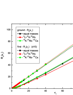
Figure 3: $R_{0}$ and $R_{1}$ as function of $\epsilon_{3}$ for three sets of mass ratios corresponding to ⁶Li⁴⁰K⁸⁷Rb and ⁴⁰K⁸⁷Rb¹³³Cs. The curves for the excited state show $10R_{1}(10\epsilon_{3})$ in order to fit within the same range as the results for the ground state.

IV Parametrization.

The universal functions, $F_{n}$, defined in Eq. (1) are not easily found analytically. However, the contour diagrams in Fig. 2 suggest a simple implicit dependence in terms of an extended Lamé curve or superellipse lame1818 . Note that despite the log-log scale of Fig. 2, the parametrization in terms of Lamé curves is done with the energies on a linear scale. The three-body energies can be written indirectly by supercircles, i.e.

$$\epsilon_{ac}^{t_{n}}+\epsilon_{bc}^{t_{n}}=R_{n}^{t_{n}}\;,$$ (3)

where the radius, $R_{n}$, and the power, $t_{n}$, are functions of $\epsilon_{3}$ and both depend on the two mass ratios. The term supercircle has been adopted since there is a single axis parameter, $R_{n}$. The smallest value of $\epsilon_{3}$ is unity corresponding to the two-body threshold of the $ab$ system used as the energy unit.

We choose sets of masses of current interest, and present the fitted radius functions in Fig. 3 for both ground and first excited states. In ⁶Li⁴⁰K⁸⁷Rb a second excited state exists whereas equal mass and ⁴⁰K⁸⁷Rb¹³³Cs only have stable ground and first excited states. The parametrized results cannot be distinguished from the computed curves in Fig. 2. The radius functions turn out to be surprisingly simple, that is essentially linear functions of $\epsilon_{3}$, and essentially independent of the masses. For the ground state we find a slight increase of slope with increasing three-body energy. Average estimates are

$$R_{0}(\epsilon_{3})\approx 0.74\epsilon_{3}-2.5\;\;,\;\;R_{1}(\epsilon_{3}) \approx \epsilon_{3}\;.$$ (4)

The increasing functions reflect how the contours in Fig. 2 move to larger two-body energies with increasing $\epsilon_{3}$.

IV.1 Symmetric systems.

It is very satisfactory to observe this simple linear dependence which implies that the three-body energy increases linearly with a kind of average of the two two-body energy ratios. It is satisfying also because the symmetric system, where all particles are identical, has this property where two- and three-body energies are proportional in the universal limit. To approach this limit we assume that $a=b$, and Eqs. (3) and (4) imply for the ground states that $0.74\epsilon_{3}\approx 2.5+\epsilon_{ac}2^{1/t_{0}}$ When $a=b=c$, we get the known ratios $\epsilon_{3}\approx(2.5+2^{1/t_{0}})/0.74=16.52$. For the excited state we get correspondingly $\epsilon_{3}\approx 2^{1/t_{1}}=1.267$. This is achieved with $t_{0}\approx 0.30$ and $t_{1}\approx 2.93$.

A system with particles $a$ and $c$ identical has been studied in Ref. bel11 . Here $\epsilon_{bc}=1$ and we can find $\epsilon_{3}$ from Eqs.(3) and (4). We get the leading order terms for $\epsilon_{3}$ to be $\epsilon_{ac}/0.74$ and $\epsilon_{ac}$ for large $\epsilon_{ac}$, respectively for ground and excited states. For small $\epsilon_{ac}$ we find correspondingly that $\epsilon_{3}$ approaches the constants $3.5/0.74$ and $1$. These leading order terms can be supplemented by further expansion to any desired order. The main dependence of the parametrization is consistent with the numerical results in bel11 .

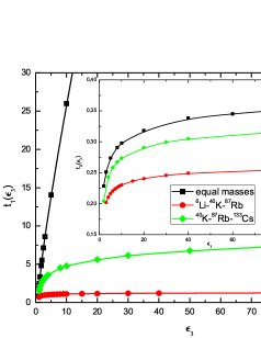
Figure 4: Exponents, $t_{1}$ and $t_{0}$ (inset) in the supercircle fit for ⁶Li⁴⁰K⁸⁷Rb and ⁴⁰K⁸⁷Rb¹³³Cs as in Fig. 3.

IV.2 The exponents.

The exponents, $t_{n}$, are crucial to obtain the correct curvature of the energy contours in Fig. 2. In Fig. 4 we show the functions obtained for the same sets of masses as in Fig. 3. These exponents increase monotonously with $\epsilon_{3}$ from $0.2$ ($n=0$) and $1$ ($n=1$) at the minimum value of $\epsilon_{3}=1$. The curves bend over and eventually stop when the states reach a two-body threshold and become unstable. In most cases this only happens at large energies where the universal properties are very unlikely.

The absolute sizes increase by about an order of magnitude from ground to first excited state. The role of the exponents in Eq. (3) is to describe the curvature of the contours in Fig. 2. Thus, large $t_{n}$ is necessary for strongly bending curves. This explains the difference between ground and first excited state, but also the overall increase with $\epsilon_{3}$. This is especially pronounced for the excited states which are squeezed in between boundaries defined by stability towards decay to bound two-body subsystems.

The contours connect boundaries with small $\epsilon_{ac}$ and large $\epsilon_{bc}$ or vice versa. The end-points are when either $\epsilon_{bc}$ or $\epsilon_{ac}$ is close to $\epsilon_{3}$. The slopes are from Eq. (3) found to be, $\partial\epsilon_{ac}/\partial\epsilon_{bc}=-(\epsilon_{bc}/\epsilon_{ac})^{t_{n}-1}$. This means that the contours in Fig. 2 first exhibit a small negative slope (small $\epsilon_{bc}$) and then a quick bend to reach a large negative slope (small $\epsilon_{ac}$). All contours decrease from left to right. The regions become narrower for higher two- and three-body energies, and the contours must bend quickly. The implication is that $t_{n}$ must increase with $\epsilon_{3}$ and with the number of excited states.

The allowed regions for a specific number of bound states are indicated in Fig. 1. The practical examples selected for Figs. 3 and 4 are found in the center, and in regions II and III of the third quadrant. In Fig. 2 the boundaries for two bound states are rather widely separated giving rise to the smallest exponents in Fig. 4. Moving towards more bound states in Fig. 1 would widen this region and the narrow strip with three bound states as well. At some point one more bound state appears but in the process all regions widened and the exponents in the fits consequently decrease. The other cases in Figs. 3 and 4 are both in region II of Fig. 1 but the point for equal masses is further away from the boundary to a region III than the point of asymmetric masses. This is a general explanation of the hierarchy in the sizes of the exponents.

The behavior of the exponents is also surprisingly simple for each set of masses. The relatively fast increase at small energies in Fig. 4 slows down and both $t_{0}$ and $t_{1}$ approach constants at large energy. For the ground state, this can be accurately captured by

$$t_{0}(\epsilon_{3})\approx\alpha_{0}\frac{\epsilon_{3}^{p_{0}}+\beta_{0}}{\epsilon_{3}^{p_{0}}+\gamma_{0}},$$ (5)

where $\alpha_{0}$ and $\alpha_{1}$ are the mass dependent constants approached at large energy, see Fig. 4. The parameters, $(p_{0},\alpha_{0})\simeq(0.04-0.06,0.3-0.5)$, exhibits a small mass dependence, whereas $(\beta_{0},\gamma_{0})\simeq-(0.93-0.95),-(0.82-0.87)$ are slightly negative but almost mass independent. We emphasize that stability requires $\epsilon_{3}>1$. The value of $t_{0}$ for small $\epsilon_{3}\approx 1$ is then in the range of $t_{0}\simeq 0.2-0.5$ as required to give the limiting value of $\epsilon_{3}=16.52$. A similar parametrization for the exponent corresponding to the excited state can be found.

V Conclusions and perspectives.

The general spectrum for three interacting particles in the universal regime in two dimensions is currently unknown. In the simplest case of three identical bosons, there is a lack of analytical results and one must resort to a numerical treatment at the moment. We numerically compute the universal three-body energies for short-range interactions, different masses and interaction strengths. The number of bound states varies from one and up depending on mass ratios and two-body subsystem energies, with symmetric system having the fewest and the most for two heavy and a light particle. The three-body ground state energies can be successfully parametrized by universal functions that are so-called supercircles (powers different from two) where the coordinates are the independent two-body energy ratios and the radius parameter is the three-body energy. The latter is an approximately linear function of the three-body energy, independent of masses, while the powers of the coordinates are functions of both mass and three-body energy. The simple threshold behavior for identical bosons where the two three-body bound states are directly proportional is only valid for relatively small three-body energies. Whether this indicates a smaller universal region has to be investigated by either finite range models or radius computations. Our results can be used as estimates of three-body energies and number of bound states, and as a measure of the deviation from the universal zero-range limit.

Acknowledgments

This work was partly support by funds provided by FAPESP (Fundação de Amparo à Pesquisa do Estado de São Paulo) and CNPq (Conselho Nacional de Desenvolvimento Científico e Tecnológico ) of Brazil.

References

- (1) L. D. Landau and E. M. Lifshitz, Quantum Mechanics (Butterworth-Heinemann, Oxford, 1977).
- (2) A. G. Volosniev, D. V. Fedorov, A. S. Jensen, and N. T. Zinner, Phys. Rev. Lett. 106, 250401 (2011).
- (3) C. Chin, R. Grimm, P. S. Julienne, and E. Tiesinga, Rev. Mod. Phys. 82, 1225 (2010).
- (4) T. Kraemer et al., Nature 440, 315 (2006).
- (5) F. Ferlaino and R. Grimm, Physics 3, 9 (2010).
- (6) A. S. Jensen, K. Riisager, D. V. Fedorov, and E. Garrido, Rev. Mod. Phys. 76, 215 (2004).
- (7) S. Tan, Ann. Phys. 323, 2952 (2008); ibid 323, 2971 (2008); 323, 2987 (2008).
- (8) J. T. Stewart, J. P. Gaebler, T. E. Drake, and D. S. Jin, Phys. Rev. Lett. 104, 235301 (2010).
- (9) E. D. Kuhnle et al., Phys. Rev. Lett. 105, 070402 (2010).
- (10) K. Martiyanov, V. Makhalov, and A. Turlapov, Phys. Rev. Lett. 105, 030404 (2010)
- (11) B. Fröhlich et al., Phys. Rev. Lett. 106, 105301 (2011).
- (12) P. Dyke et al., Phys. Rev. Lett. 106, 105304 (2011).
- (13) R. Combescot, F. Alzetto and X. Leyronas, Phys. Rev. A 79, 053640 (2009).
- (14) F. Werner and Y. Castin, arXiv:1001.0774 (2010).
- (15) M. Valiente, N. T. Zinner, and K. Mølmer, Phys. Rev. A 84, 063626 (2011).
- (16) C. Langmack, M. Barth, W. Zwerger and E. Braaten, arXiv:1111.0999 (2011).
- (17) J. A. Tjon, Phys. Lett. B 56, 217 (1975).
- (18) S. K. Adhikari, A. Delfino, T. Frederico, I. D. Goldman, and L. Tomio, Phys. Rev. A 37, 3666 (1988); S. K. Adhikari, A. Delfino, T. Frederico, and L. Tomio, Phys. Rev. A 47, 1093 (1993).
- (19) E. Nielsen, D. V. Fedorov, and A. S. Jensen, Phys. Rev. A 56, 3287 (1997).
- (20) E. Nielsen, D. V. Fedorov, A. S. Jensen, and E. Garrido, Phys. Rep. 347, 373 (2001).
- (21) I. V. Brodsky, M. Yu Kagan, A. V. Klaptsov, R. Combescot, and Y. Leyronas, Phys. Rev. A 73, 032724 (2006).
- (22) O. I. Kartavtsev and A. V. Malykh, Phys. Rev. A 74, 042506 (2006).
- (23) L. Platter, H.-W. Hammer, and U.-G. Meißner, Few-Body Syst. 35, 165 (2004).
- (24) K. Helfrich and H.-W. Hammer, Phys. Rev. A 83, 052703 (2011).
- (25) H.-W. Hammer and D. T. Son, Phys. Rev. Lett. 93, 250408 (2004).
- (26) D. Blume, Phys. Rev. B 72, 094510 (2005).
- (27) D. Lee, Phys. Rev. A 73, 063204 (2006).
- (28) V. Efimov, Yad. Fiz 12, 1080 (1970); Sov. J. Nucl. Phys. 12, 589 (1971).
- (29) C.-H. Wu, I. Santiago, J. W. Park, P. Ahmadi, and M. W. Zwierlein, Phys. Rev. A 84, 011601(R) (2011).
- (30) F. Bellotti et al., J. Phys. B: At. Mol. Opt. Phys. 44, 205302 (2011).
- (31) E. Braaten and H. W. Hammer, Phys. Rep. 428, 259 (2006).
- (32) G. Lamé: Examen des différentes méthodes employées pour résoudre les problémes de géométrie, (Vve Courcier, 1818).
- (33) F. Bellotti et al., in preparation.
- (34) M.T. Yamashita, T. Frederico, A. Delfino and L. Tomio, Phys. Rev. A 66, 052702 (2002).