Interior Regularity Estimates in High Conductivity Homogenization and Application

Abstract

In this paper, uniform pointwise regularity estimates for the solutions of conductivity equations are obtained in a unit conductivity medium reinforced by a $\varepsilon$-periodic lattice of highly conducting thin rods. The estimates are derived only at a distance $\varepsilon^{1+\tau}$ (for some $\tau>0$) away from the fibres. This distance constraint is rather sharp since the gradients of the solutions are shown to be unbounded locally in $L^{p}$ as soon as $p>2$. One key ingredient is the derivation in dimension two of regularity estimates to the solutions of the equations deduced from a Fourier series expansion with respect to the fibres direction, and weighted by the high-contrast conductivity. The dependence on powers of $\varepsilon$ of these two-dimensional estimates is shown to be sharp. The initial motivation for this work comes from imaging, and enhanced resolution phenomena observed experimentally in the presence of micro-structures LEROSEY-ET-AL-07 . We use these regularity estimates to characterize the signature of low volume fraction heterogeneities in the fibred reinforced medium assuming that the heterogeneities stay at a distance $\varepsilon^{1+\tau}$ away from the fibres.

AMS subject classification: 35J15 - 35B27 - 35B65

1 Introduction

Consider a material contained in $\Omega$ ${}=$ ${\omega}\times(-L,L)\,\subset\,{\mathbb{R}}^{3}$ where ${\omega}$ is a bounded domain in ${\mathbb{R}}^{2}$ with smooth boundary $\partial{\omega}$. Given some fixed $\omega_{0}\Subset{\omega}$, we assume that inside ${\Omega_{0}}=\omega_{0}\times(-L,L)$, the material contains small cylindrical rods of high conductivity.

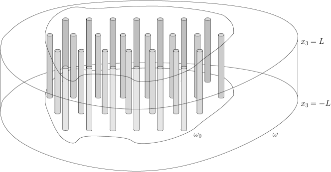
Figure 1: Sketch of a domain $\Omega=\omega\times(-L,L)$ containing cylindrical rods.

A sketch of the domain is represented in Figure 1. For $\varepsilon>0$, $r_{\varepsilon}\ll\varepsilon$, and $(m,n)\in{\mathbb{Z}}^{2}$, let

$$D_{m,n,\varepsilon} {}=D_{\varepsilon r_{\varepsilon}}(m\varepsilon,n\varepsilon)\;,$$

$$Q_{m,n,\varepsilon} {}=D_{m,n,\varepsilon}\times(-L,L)\;,$$

where $D_{\varepsilon r_{\varepsilon}}(m\varepsilon,n\varepsilon)$ is the disc of radius $\varepsilon r_{\varepsilon}$ centered at $(m\varepsilon,n\varepsilon)$. Introduce the index set

$$I_{\varepsilon}{}=\{(m,n)\in{\mathbb{Z}}^{2}:D_{m,n,\varepsilon}\subset\omega_{0}\}\;,$$

and set

$$D_{\varepsilon}{}=\bigcup_{(m,n)\in I_{\varepsilon}}D_{m,n,\varepsilon}\;,\qquad Q_{\varepsilon}{}=\bigcup_{(m,n)\in I_{\varepsilon}}Q_{m,n,\varepsilon}\;.$$

We will assume that the conductivity parameter of ${\Omega}$ is of the form

$$a_{\varepsilon}{}=\left\{\begin{array}[]{ll}1&\text{ in }{\Omega}\setminus Q_{\varepsilon}\;,\\ \alpha_{\varepsilon}&\text{ in }Q_{\varepsilon}\;,\end{array}\right.$$ (1)

where

$$0<\kappa_{-}\leq\alpha_{\varepsilon}\,\pi r_{\varepsilon}^{2}\leq\kappa_{+}\;.$$ (2)

Additionally, we assume

$$0<\frac{2\pi}{\gamma_{+}}\leq-\varepsilon^{2}\ln r_{\varepsilon}\,\leq\frac{2\pi}{\gamma_{-}}\;.$$ (3)

We consider, for $\Phi_{b}\in C^{1}(\bar{\Omega})$ and $F$ $\in$ $L^{2}({\Omega})$, the solution $\Psi_{\varepsilon}\in H^{1}({\Omega})$ of

$$\left\{\begin{array}[]{ll}-{\rm div}(a_{\varepsilon}\,\nabla\Psi_{\varepsilon})=F&\text{ in }{\Omega}\;,\\ \Psi_{\varepsilon}=\Phi_{b}&\text{ on }\partial{\Omega}\;.\end{array}\right.$$ (4)

This model, initially introduced by Fenchenko & Khruslov FENCHENKO-KHRUSLOV-81 , has been studied in the context of homogenization by several authors KHRUSLOV-91 ; BELLIEUD-BOUCHITTE-98 ; BRIANE-TCHOU-01 ; BRIANE-03 ; MARCHENKO-KHRUSLOV-06 . It is known to have a non-standard behaviour when $\varepsilon$ tends to zero. Namely, the homogenized limit is not of divergence form, and admits a non-local term (see Theorem 2.3 for the precise form of the limit). While it is clear that, thanks to the ellipticity, a global $W^{1,2}\left(\Omega\right)$ bound holds, one can show that except for special boundary data $\Phi_{b}$, the solutions $\Psi_{\varepsilon}$ of (4) are unbounded in $W^{1,p}_{\rm loc}({\Omega}_{0})$ for any $p>2$, see Corollary 2. This makes the situation very different from the case of bounded coefficients: Meyers’ Theorem MEYERS-63 shows that solutions are bounded in $W^{1,p}_{\rm loc}$ for some $p>2$ in that case. In the case of periodic composites with bounded coefficients, Li & Vogelius LI-VOGELIUS-00 and Li & Nirenberg LI-NIRENBERG-03 showed one can in fact obtain $W^{1,\infty}$ estimates. However, such improved regularity estimates strongly depend on the contrast of the coefficients as shown for example in LEONETTI-NESI-97 ; AMMARI-KANG-LIM-05 ; BAO-LI-YIN-09 .

The first goal of this work is to establish interior $C^{1,\alpha}$ estimates, uniformly in $\varepsilon$, for $\Psi_{\varepsilon}$ away from $Q_{\varepsilon}$. We show that in a set $\Omega_{\varepsilon}=\omega_{\varepsilon}\times(-l,l)$ improved regularity estimates can be obtained. The set ${\omega}_{\varepsilon}$ is “almost” the complement of the high conductivity fibres in the sense that $\omega_{\varepsilon}\cap D_{\varepsilon}=\emptyset$ and $\omega_{0}\setminus\omega_{\varepsilon}$ tends to zero with $\varepsilon$. Introducing $V$ the solution in $H_{0}^{1}(\Omega)$ of

$$-\Delta V=F,$$

we show that

$$\|\Psi_{\varepsilon}-V\|_{C^{1,\nu}\left(\Omega_{\varepsilon}\right)}\leq C\,\|F\|_{L^{2}({\Omega})},$$

see Theorems 2.1 and 2.2 for precise statements.

We can think of several applications for this work. One could for example use this result to establish a posteriori error estimates for the numerical solutions of (4). Our initial motivation came from a question related to imaging. In a recent work, Ammari et al. AMMARI-BONNETIER-CAPDEBOSCQ-09 showed that the signature of small inclusions inside a periodic medium was determined by the effective properties of this medium, in the limit when both the period and the size of the inclusions tend to zero. The motivation for this study was to provide a mathematical perspective on the so-called “resolution beyond the diffraction limit” verified experimentally LEROSEY-ET-AL-07 .

Recent developments in material sciences, see Bouchitté et al. BOUCHITTE-BOUREL-FELBACQ-09 , have shown that very high contrast composite materials, with scalings similar to the ones used in this paper, could be used to construct meta-materials with particularly interesting properties (such as materials with negative optical indices). Such composites are out of the scope of AMMARI-BONNETIER-CAPDEBOSCQ-09 . This work relies on elliptic regularity estimates shown by Li & Nirenberg which do not apply for large contrast. These imaging problems involve either the Helmholtz equation, or the full Maxwell equation. We limited our study to the case of a real valued conductivity coefficient in this work. Assume a perturbation of small volume $G_{\varepsilon}$ is located inside $\Omega_{\varepsilon}$ with conductivity $\gamma_{1}\in C^{0}(\Omega)$. The conductivity of the defective medium is

$$a_{\varepsilon,d}{}=\left\{\begin{array}[]{ll}1&\text{ in }\Omega\setminus(Q_{\varepsilon}\cup G_{\varepsilon})\;,\\ \gamma_{1}&\text{ in }G_{\varepsilon}\;,\\ \alpha_{\varepsilon}&\text{ in }Q_{\varepsilon}\;.\end{array}\right.$$ (5)

For $\Phi_{b}\in C^{1}(\bar{\Omega})$, consider $W_{\varepsilon,d}$ the solution of

$$\left\{\begin{array}[]{ll}{\rm div}(a_{\varepsilon,d}\,\nabla W_{\varepsilon,d})=0&\text{ in }\Omega\;,\\ W_{\varepsilon,d}=\Phi_{b}&\text{ on }\partial\Omega\;,\end{array}\right.$$ (6)

and compare it to the unperturbed solution $W_{\varepsilon}$ of

$$\left\{\begin{array}[]{ll}{\rm div}(a_{\varepsilon}\,\nabla W_{\varepsilon})=0&\text{ in }\Omega\;,\\ W_{\varepsilon}=\Phi_{b}&\text{ on }\partial\Omega\;.\end{array}\right.$$ (7)

The signature on the boundary of the defect is characterised by the quadratic form ${{\mycal R}_{\varepsilon}}:H^{1/2}(\partial\Omega)\to\mathbb{R}$ defined by

$${{\mycal R}_{\varepsilon}}(\Phi_{b}){}=\int_{\partial\Omega}a_{\varepsilon}\frac{\partial}{\partial n}\left(W_{\varepsilon,d}-W_{\varepsilon}\right)(s)\Phi_{b}(s)ds.$$

We show in Theorem 4.1 that at first order, for $\Phi_{b}\in C^{1}(\bar{\Omega})$, it is of the form

$${{\mycal R}_{\varepsilon}}(\Phi_{b})=\left|G_{\varepsilon}\right|\int_{\Omega}M\nabla W_{*}\cdot\nabla W_{*}\,d\mu+o\left(\left|G_{\varepsilon}\right|\right),$$

where $W_{*}$ is the solution of the homogenized problem (13) associated with (7). This can be seen as an extension of CAPDEBOSCQ-VOGELIUS-03A to (7). At first order, the signature of the defect is similar to what would be observed if defect was introduced in the effective medium, instead of the homogeneous substrate: the only difference is the formula of polarisation tensor $M$. This is what was observed in BENHASSEN-BONNETIER-06 for finite conductivities.

Theorem 4.1 has another interpretation, probably of equal if not greater importance for applications. Theorem 4.1, compared with the main result of AMMARI-BONNETIER-CAPDEBOSCQ-09 or BENHASSEN-BONNETIER-06 shows that impurities in the substrate do not affect the overall properties of the composite material more than impurities would affect a regular composite, provided these impurities are located in $\Omega_{\varepsilon}$, that is, not too close to the highly conducting fibres but not necessarily at a distance proportional to the size of the microstructure. As far as the authors are aware, this is the first result of this nature. If such highly contrasted structures are used to manufacture meta-materials, as it is suggested in BOUCHITTE-BOUREL-FELBACQ-09 , this result is of practical importance.

Another very related question is the regularity of the solution of a problem similar to (4), where cavities replace inclusions. This problem shows a similar non-standard effective behaviour, the celebrated “strange term” of Cioranescu and Murat CIORANESCU-MURAT-82 . This will be the subject of a forthcoming paper.

Our paper is structured as follows. In Section 2, we state our main results concerning the regularity of (4) away from the highly conductive fibres. First, we consider for $F$ $\in$ $L^{2}({\Omega})$, the solution $U_{\varepsilon}\in H_{0}^{1}({\Omega})$ of

$$\left\{\begin{array}[]{ll}-{\rm div}(a_{\varepsilon}\,\nabla U_{\varepsilon})=F&\text{ in }{\Omega}\;,\\ U_{\varepsilon}=0&\text{ on }\partial{\Omega}\;.\end{array}\right.$$ (8)

Our result concerning problem (8) is Theorem 2.1. We then turn to the boundary value problem (7), and obtain an estimate for $W_{\varepsilon}$ in Theorem 2.2. To highlight the fact that excluding a buffer zone around the highly conducting fibres is necessary, for any $p>2$ we provide an explosive lower bound for the $W^{1,p}$ norm of $W_{\varepsilon}$ in Corollary 2 (see also Remark 3). This result is a corollary of the homogenization result given by Theorem 2.3.

Our approach relies on the fact that one can perform a partial Fourier series decomposition of $U_{\varepsilon}$ and $W_{\varepsilon}$ in $x_{3}$. In Section 3 we prove Theorem 2.1 and Theorem 2.2 starting from the regularity of the Fourier coefficients. Note that translating the interior regularity results from $U_{\varepsilon}$ to $W_{\varepsilon}$ is not obvious. A natural idea is to study $\tilde{W}_{\varepsilon}=\eta W_{\varepsilon}$, where $\eta$ is a cut-off function. Provided the cut-off function is chosen carefully, this leads to an interior problem in $H^{1}_{0}({\Omega})$,

$$-{\rm div}(a_{\varepsilon}\,\nabla\tilde{W}_{\varepsilon})=-2a_{\varepsilon}\nabla W_{\varepsilon}\cdot\nabla\eta-a_{\varepsilon}\Delta\eta W_{\varepsilon}\text{ in }{\Omega}.$$

Let us focus on the first right-hand side term. Remembering that the only bound uniform in $\varepsilon$ is the energy bound, $\int_{\Omega}a_{\varepsilon}|\nabla W_{\varepsilon}|^{2}\leq C\|\Phi_{b}\|_{C^{1}(\bar{\Omega})}$, since $\nabla W_{\varepsilon}$ is not bounded uniformly in $\varepsilon$ in any $L^{p}({\Omega})$ for $p>2$, we are then left with a problem of the form

$$-{\rm div}(a_{\varepsilon}\,\nabla\hat{W}_{\varepsilon})=-a_{\varepsilon}f,\mbox{ in }H^{1}_{0}(\Omega)\mbox{ with }\int_{\Omega}a_{\varepsilon}f^{2}dx<\infty.$$

Unfortunately, without additional information on $f$, this is not enough to guarantee that $\hat{W}_{\varepsilon}$ is bounded in $L^{\infty}(\Omega)$. In Proposition 4, we show that the best one can hope for in this case is $\varepsilon\|\hat{W}_{\varepsilon}\|_{L^{\infty}}<C\|\sqrt{a_{\varepsilon}}f\|_{L^{2}}$.

In Section 4, we show how these results can be used to obtain a representation formula for inclusions of small measure located away from the fibres. This part was the initial motivation of this work. Because outside of the highly conducting fibres the substrate is homogeneous, we provide a self-contained proof.

We prove the homogenization Theorem 2.3 in Section 5, and finally turn to more technical results. Section 6 is devoted to the proof of Lemma 1, a supremum estimate of de Giorgi-Moser-Nash type adapted to our problem. The proof of this Lemma uses a Poincaré-Sobolev inequality proved in Lemma 4. Section 7 contains the proof of the regularity results for the Fourier coefficients associated with $U_{\varepsilon}$. Section 8 is the counterpart of Section 7, for $W_{\varepsilon}$. Several intermediate technical results are proved in Appendix A.

2 Main interior regularity estimates

The main part of this paper is devoted to the derivation of interior regularity estimates for problem (4), outside of the highly conducting rods.

For a fixed $\omega_{0}\Subset\omega_{1}\Subset{\omega}$, define ${\omega}_{\tau}^{\varepsilon}$ by

$${\omega}_{\tau}^{\varepsilon}{}=\{x\in\omega_{1}:{\rm dist}\,(x,D_{\varepsilon})\geq\varepsilon\tau\}.$$ (9)

Our result concerning problem (8) is the following.

Theorem 2.1

For $\kappa>0$, $\tau>\kappa\,\varepsilon^{\frac{1-\eta}{2(1+\eta)}}$ with $\eta\in\left(\frac{3}{4},1\right)$, and $0<\nu<2\left(\eta-\frac{3}{4}\right)$, the solution $U_{\varepsilon}$ of (8) satisfies

$$\left\|U_{\varepsilon}-V\right\|_{C^{1,\nu}\left({\omega}_{\tau}^{\varepsilon}\times(-L,L)\right)}\leq C(\kappa,\eta,\nu)\|F\|_{L^{2}(\Omega)},$$

where $V\in H^{1}_{0}(\Omega)$ is the solution of

$$-\Delta V=F.$$

This result is proved in Section 3.

Remark 1

It should be noted that, generically, $V$ may not belong to any $W^{1,p}(\Omega)$ for $p>6$. The above result asserts that the difference $U_{\varepsilon}-V$ enjoys a better regularity in most of the domain since $|\omega_{1}\setminus{\omega}_{\tau}^{\varepsilon}|\rightarrow 0$ as $\varepsilon\rightarrow 0$.

We use the notation $C$ for various constants in the paper which are always independent of $\varepsilon$. When appropriate, we highlight the dependence on the parameters appearing in the statements of the results by writing $C(a,b,\ldots)$.

As a direct consequence of the above theorem, we have

Corollary 1

Under the assumptions of Theorem 2.1 we have

$$\left\|U_{\varepsilon}\right\|_{L^{\infty}\left({\omega}_{\tau}^{\varepsilon}\times(-L,L)\right)}+\left\|\nabla U_{\varepsilon}\right\|_{L^{6}\left({\omega}_{\tau}^{\varepsilon}\times(-L,L)\right)}\leq C(\kappa,\eta)\|F\|_{L^{2}(\Omega)}.$$ (10)

Next, we derive an estimate for the solution $W_{\varepsilon}$ of (7), given by the following proposition.

Theorem 2.2

Let $\Omega_{\tau}^{\varepsilon}{}={\omega}_{\tau}^{\varepsilon}\times(-l,l)$, with $l<L$. For $\kappa>0$, $\tau>\kappa\,\varepsilon^{\frac{1-\eta}{2(1+\eta)}}$ with $\eta\in\left(\frac{3}{4},1\right)$, and $0<\nu<2\left(\eta-\frac{3}{4}\right)$, the solution $W_{\varepsilon}$ of (7) satisfies

$$\|W_{\varepsilon}\|_{C^{1,\nu}\left(\Omega_{\tau}^{\varepsilon}\right)}\leq C(\kappa,\eta,\nu,l)\,\|\Phi_{b}\|_{C^{1}(\bar{\Omega})}.$$

This result is proved in Section 3.

Remark 2

Once again, as $\varepsilon\rightarrow 0$, we have $|\omega_{1}\setminus{\omega}_{\tau}^{\varepsilon}|=o(1)$, therefore the solution of (8) enjoys a uniform $C^{1,\nu}$-bound in almost the whole domain.

It is natural to ask whether a uniform global $C^{1,\nu}$-bound exists for $\Omega$. To answer this question, first we consider the limit homogenized problem corresponding to (7). To state our homogenization result, we need to introduce a capacity function. The function ${c_{\varepsilon}^{\sigma}}$ is defined, for some $\sigma\geq 1$, in ${\Omega}$ by

$${c_{\varepsilon}^{\sigma}}(x){}=\left\{\begin{array}[]{cl}0&\mbox{if }r=\sqrt{(x_{1}-m\varepsilon)^{2}+(x_{2}-n\varepsilon)^{2}}\leq\varepsilon r_{\varepsilon}\\[3.99994pt] \displaystyle\frac{\ln r-\ln(\varepsilon r_{\varepsilon})}{\ln(\varepsilon^{\sigma}/2)-\ln(\varepsilon r_{\varepsilon})}&\mbox{if }r\in(\varepsilon r_{\varepsilon},\varepsilon^{\sigma}/2),\quad\mbox{for }(m,n)\in I_{\varepsilon},\\[3.99994pt] 1&\mbox{elsewhere}.\end{array}\right.$$ (11)

In fact, we choose $\sigma$ so that $\varepsilon^{\sigma}>\varepsilon\,\tau$. Note that ${c_{\varepsilon}^{\sigma}}$ does not depend on the variable $x_{3}$, is periodic of period $[-\varepsilon/2,\varepsilon/2]^{3}$ in ${\Omega_{0}}$, and is equal to $1$ outside of ${\Omega_{0}}$. This capacity function has been ubiquitous in the derivation of homogenization results related to conductivities of the form (1) since its introduction in CIORANESCU-MURAT-82 .

We have the following homogenization result, proved in Section 5. Note that $a_{\varepsilon}$ is only reinforced in the cylinder ${\Omega_{0}}=\omega_{0}\times(-L,L)$.

Theorem 2.3

Assume in addition to (2), (3), that

$$\lim_{\varepsilon\to 0}\;\alpha_{\varepsilon}\,\pi r_{\varepsilon}^{2}=\kappa\in[\kappa_{-},\kappa_{+}],\quad\lim_{\varepsilon\to 0}\;\frac{2\pi}{\varepsilon^{2}\left|\ln r_{\varepsilon}\right|}=\gamma\in[\gamma_{-},\gamma_{+}].$$ (12)

Let $\Phi_{b}\in C^{1}(\bar{\Omega})$. Then, the solution $W_{\varepsilon}$ converges weakly in $H^{1}({\Omega})$ to the unique solution $W_{*}$ of the coupled system

$$\left\{\begin{array}[]{rl}\displaystyle-\,\Delta W_{*}+\gamma\left(W_{*}-V_{*}\right)1_{\Omega_{0}}=0&\mbox{in }\Omega\\[6.00006pt] -\,\kappa\,\partial^{2}_{33}V_{*}+\gamma\left(V_{*}-W_{*}\right)=0&\mbox{in }\Omega_{0}=\omega_{0}\times(-L,L)\\[3.99994pt] W_{*}=\Phi_{b}&\mbox{on }\partial{\Omega}\\[3.99994pt] V_{*}(\cdot,\pm L)=\Phi_{b}(\cdot,\pm L)&\mbox{in }\omega_{0}.\end{array}\right.$$ (13)

The pair $(W_{*},V_{*})$ satisfies $W_{*}\in C^{0,\alpha}(\bar{\Omega})\cap W^{2,p}_{\rm loc}({\Omega})$ and $V_{*}\in C^{0,\alpha}(\bar{\Omega}_{0})\cap C^{\infty}_{\rm loc}(\Omega_{0})$ for some $\alpha\in(0,1)$ and for any $p>2$.

Moreover, the following corrector result holds:

$$\lim_{\varepsilon\to 0}\;\int_{\Omega}a_{\varepsilon}\big{|}\nabla W_{\varepsilon}-\nabla{c_{\varepsilon}^{\sigma}}\left(W_{*}-V_{*}\right)-{c_{\varepsilon}^{\sigma}}\nabla W_{*}-(1-{c_{\varepsilon}^{\sigma}})\,\partial_{3}V_{*}\,e_{3}\big{|}^{2}\,dx=0.$$ (14)

Because of the non-local nature of the problem it solves, it is not clear that $W_{*}$ is analytic inside ${\Omega_{0}}$. The following proposition shows that it enjoys partial analyticity, that is, with respect to the $x_{3}$ variable.

Proposition 1

Under the hypothesis of Theorem 2.3, the solutions $W_{*}$ and $V_{*}$ of (13) are analytic with respect to the $x_{3}$ variable in ${\Omega_{0}}$.

This result is proved in Appendix A.1. We are now in position to answer the global regularity question. Theorem 2.3 and Proposition 1 imply that one cannot expect an $\varepsilon$ independent bound for the sequence $W_{\varepsilon}$ in a space better than $H^{1}({\Omega})$ in general, as the following Corollary shows.

Corollary 2

Let $\Phi_{b}\in C^{2}(\bar{{\Omega}})$ be such that the sets

$$S_{\pm}(\Phi_{b})=\left\{x^{\prime}\in\omega_{0}\mbox{ such that }\Delta_{2}\Phi_{b}(\cdot,\pm L)=0\right\},\quad\mbox{where }\Delta_{2}=\partial^{2}_{11}+\partial^{2}_{22},$$

have an intersection of zero measure. Then, the sequence $W_{\varepsilon}$ is unbounded in $W^{1,p}_{\rm loc}({\Omega_{0}})$ for any $p>2$. More precisely, for any non empty open set $\Omega^{\prime}\subset\Omega_{0}$, there exists a positive constant $C(\Omega^{\prime},\Phi_{b})$ independent of $\varepsilon$ such that for any $\rho\in(0,1)$ and $p>2$,

$$\liminf_{\varepsilon\to 0}\left(r_{\varepsilon}^{2\rho(1-2/p)}\|\nabla W_{\varepsilon}\|_{L^{p}(\Omega^{\prime}\setminus Q_{\varepsilon})}^{2}\right)\geq(1-\rho)C\left(\Omega^{\prime},\Phi_{b}\right).$$

Proof

Working with a subsequence if necessary, we can assume that (12) holds.

Fix $\rho\in(0,1)$ and let $\mathcal{O}_{\varepsilon}$ be the open subset of ${\Omega_{0}}$ defined by

$$\mathcal{O}_{\varepsilon}=\big{\{}x\in\omega_{0}:0<{\rm dist}\,(x,D_{\varepsilon})<\varepsilon r_{\varepsilon}^{\rho}\big{\}}\times(-L,L),$$ (15)

By the definition (11) of ${c_{\varepsilon}^{\sigma}}$ combined with (12), and by the periodicity of ${c_{\varepsilon}^{\sigma}}$ and $\mathbf{1}_{\mathcal{O}_{\varepsilon}}$ in ${\Omega_{0}}$, we have

$$1_{\mathcal{O}_{\varepsilon}}\,|\nabla{c_{\varepsilon}^{\sigma}}|^{2}\;\rightharpoonup\;\lim_{\varepsilon\to 0}\left(\frac{2\pi}{\varepsilon^{2}}\int_{\varepsilon r_{\varepsilon}}^{\varepsilon r_{\varepsilon}^{\rho}}\frac{dr}{r\,\ln^{2}(2\varepsilon^{1-\sigma}\,r_{\varepsilon})}\right)=\gamma(1-\rho)\quad\mbox{weakly-}*\mbox{ in }\mathcal{M}({\Omega_{0}}),$$

which by virtue of the continuity of $V_{*}-W_{*}$ implies that

$$1_{\mathcal{O}_{\varepsilon}}\,|\nabla{c_{\varepsilon}^{\sigma}}|^{2}\,(V_{*}-W_{*})^{2}\,dx\;\rightharpoonup\;\gamma(1-\rho)\,(V_{*}-W_{*})^{2}\quad\mbox{weakly-}*\mbox{ in }\mathcal{M}({\Omega_{0}}).$$ (16)

Let us show that this last term does not cancel on any non-empty open subset $\Omega^{\prime}\subset\Omega_{0}$. By contradiction, suppose that the continuous function $V_{*}-W_{*}\equiv 0$ on a ball $B_{R}(p^{0})$, centred in $p^{0}=(p^{0}_{1},p^{0}_{2},p^{0}_{3})$ and of radius $R>0$, such that $B_{R}(p_{0})\subset\Omega_{0}$. This implies that for example that for any $x^{\prime}\in C_{R}$, with $C_{R}=(p^{0}_{1}-R/2,p^{0}_{1}+R/2)\times(p^{0}_{2}-R/2,p^{0}_{2}+R/2)$, the function $W_{*}(x^{\prime},\cdot)-V_{*}(x^{\prime},\cdot)$ is identically zero on $(p^{0}_{3}-\sqrt{3}R/2,p^{0}_{3}+\sqrt{3}R/2)$. As we have shown in Proposition 1, this function is analytic on $(-L,L)$ therefore $W_{*}=V_{*}$ on $C_{R}\times(-L,L)$. The system (13) then shows that $\partial^{2}_{33}V_{*}=\Delta V_{*}=\Delta W_{*}=0$ in $C_{R}\times(-L,L)$. Hence, taking into account the boundary conditions of (13) we would have

$$W_{*}(x)=V_{*}(x)=\frac{L+x_{3}}{2L}\,\Phi_{b}(x^{\prime},L)+\frac{L-x_{3}}{2L}\,\Phi_{b}(x^{\prime},-L)\quad\mbox{for any }x\in C_{R}\times(-L,L).$$

Since $W_{*}$ is harmonic in $C_{R}\times(-L,L)$, it follows that both functions $\Phi_{b}(\cdot,\pm L)$ are harmonic in $C_{R}$, therefore $|S_{+}(\Phi_{b})\cap S_{-}(\Phi_{b})|\geq|C_{R}|>0$ which contradicts the hypothesis.

Next, since $\nabla W_{*},\partial_{3}V_{*}\in L^{2}({\Omega_{0}})$ and $0\leq{c_{\varepsilon}^{\sigma}}\leq 1$ in ${\Omega_{0}}$, we have

$$\lim_{\varepsilon\to 0}\int_{\mathcal{O}_{\varepsilon}}\big{|}{c_{\varepsilon}^{\sigma}}\nabla W_{*}+(1-{c_{\varepsilon}^{\sigma}})\,\partial_{3}V_{*}\,e_{3}\big{|}^{2}\,dx=0.$$

Hence, by the convergence (14) and the fact that $a_{\varepsilon}\equiv 1$ in $\mathcal{O}_{\varepsilon}$, we deduce that

$$1_{\mathcal{O}_{\varepsilon}}\big{|}\nabla W_{\varepsilon}-\nabla{c_{\varepsilon}^{\sigma}}\left(W_{*}-V_{*}\right)\big{|}^{2}\;\longrightarrow\;0\quad\mbox{strongly in }L^{1}_{\rm loc}({\Omega_{0}}).$$

This combined with convergence (16) implies that

$$1_{\mathcal{O}_{\varepsilon}}|\nabla W_{\varepsilon}|^{2}\;\rightharpoonup\;\gamma(1-\rho)(V_{*}-W_{*})^{2}\quad\mbox{weakly-}*\mbox{ in }{\mathcal{M}}({\Omega_{0}}).$$ (17)

To proceed, fix $\Omega^{\prime\prime}\Subset\Omega^{\prime}\subset\Omega_{0}$ and select a smooth cut-off function $\zeta\in C_{c}^{\infty}(\Omega^{\prime})$ such that $0\leq\zeta\leq 1$ and $\zeta\equiv 1$ in $\Omega^{\prime\prime}$. Note that, for some $C_{1}>1$

$$C_{1}^{-1}\,r_{\varepsilon}^{2\rho}\leq|\mathcal{O}_{\varepsilon}|\leq C_{1}\,r_{\varepsilon}^{2\rho}.$$

Thus, (17) shows

$$\int_{\Omega^{\prime\prime}}\gamma(1-\rho)(V_{*}-W_{*})^{2}\,dx \leq\int_{\Omega_{0}}\gamma(1-\rho)(V_{*}-W_{*})^{2}\,\zeta\,dx$$

$$=\lim_{\varepsilon\to 0}\int_{\mathcal{O}_{\varepsilon}}|\nabla W_{\varepsilon}|^{2}\,\zeta\,dx$$

$$\leq\liminf_{\varepsilon\to 0}\int_{\mathcal{O}_{\varepsilon}\cap\Omega^{\prime}}|\nabla W_{\varepsilon}|^{2}\,dx$$

$$\leq\liminf_{\varepsilon\to 0}\left(|\mathcal{O}_{\varepsilon}|^{1-2/p}\|\nabla W_{\varepsilon}\|_{L^{p}(\Omega^{\prime}\setminus Q_{\varepsilon})}^{2}\right)$$

$$\leq C_{1}\liminf_{\varepsilon\to 0}\left(r_{\varepsilon}^{2\rho(1-2/p)}\|\nabla W_{\varepsilon}\|_{L^{p}(\Omega^{\prime}\setminus Q_{\varepsilon})}^{2}\right).$$

Since this is valid for all $\Omega^{\prime\prime}\Subset\Omega^{\prime}$, we conclude the proof. ∎

Remark 3

Note that Corollary 2 shows that gradient blow-up occurs outside of the highly conducting rods. An variant of the proof shows that one can obtain the following estimate

$$\liminf_{\varepsilon\to 0}\left(r_{\varepsilon}^{2\rho(1-2/p)}\|\nabla W_{\varepsilon}\|_{L^{p}(\Omega^{\prime}\setminus\hat{Q}_{\varepsilon}^{\rho^{\prime}})}^{2}\right)\geq(\rho^{\prime}-\rho)C\left(\Omega^{\prime},\Phi_{b}\right),$$

where $0<\rho<\rho^{\prime}<1$ and

$$\hat{Q}_{\varepsilon}^{\rho^{\prime}}=\big{\{}x\in\omega_{0}:{\rm dist}\,(x,D_{\varepsilon})\leq\varepsilon r_{\varepsilon}^{\rho^{\prime}}\big{\}}\times(-L,L),$$

which shows that the blow-up is not localized on the surface of the rods.

3 Regularity estimates in two dimensions for weighted equations and three-dimensional consequences

In this section, we state the regularity results we have obtained for two-dimensional companion problems of problem (4). To highlight the sharpness of the supremum estimate provided by Lemma 1, which provides an $L^{\infty}$ upper bound of the form $C(s)\varepsilon^{-s}$ for any $2>s>1$, we construct in Proposition 4 an example where the $L^{\infty}$ norm is bounded from below by $C\epsilon^{-1}$. Then, we prove Theorem 2.1 and Theorem 2.2.

3.1 Towards the proof of Theorem 2.1

Let us now turn to the proof of Theorem 2.1. Because none of the coefficients depend on $x_{3}$, we can, as in BRIANE-CASADO-08 , reduce the study of this three-dimensional problem to that of a two-dimensional problem by separating variables. We write

$$U_{\varepsilon}(x^{\prime},x_{3}) \sim\sum_{n=1}^{\infty}u_{\varepsilon,n}(x^{\prime})\,\sin\Big{(}\frac{n\pi}{2}\big{(}\frac{x_{3}}{L}+1\big{)}\Big{)}\;,$$ (18)

$$F(x^{\prime},x_{3}) \sim\sum_{n=1}^{\infty}f_{n}(x^{\prime})\,\sin\Big{(}\frac{n\pi}{2}\big{(}\frac{x_{3}}{L}+1\big{)}\Big{)}\;,$$ (19)

and (8) becomes

$$\left\{\begin{array}[]{ll}-{\rm div}_{2}(a_{\varepsilon}\,\nabla_{2}u_{\varepsilon,n})+\frac{n^{2}\pi^{2}}{4L^{2}}\,a_{\varepsilon}\,u_{\varepsilon,n}=f_{n}&\text{ in }{\omega}\;,\\ u_{\varepsilon,n}=0&\text{ on }\partial{\omega}\;.\end{array}\right.$$ (20)

In the above, ${\rm div}_{2}$ and $\nabla_{2}$ denotes the horizontal divergence and gradient operators. We are thus led to consider, for $\lambda\geq\frac{\pi^{2}}{4L^{2}}$,

$$\left\{\begin{array}[]{ll}-{\rm div}_{2}(a_{\varepsilon}\,\nabla_{2}u_{\varepsilon})+\lambda\,a_{\varepsilon}\,u_{\varepsilon}=f+a_{\varepsilon}\,g+{\rm div}_{2}({\mathbf{h}})&\text{ in }{\omega}\;,\\ u_{\varepsilon}=0&\text{ on }\partial{\omega}\;,\end{array}\right.$$ (21)

where $f\in L^{2}(\omega)$, $\sqrt{a_{\varepsilon}}g\in L^{2}(\omega)$ and $h\in L^{\infty}(\omega)^{2}$. Problem (21) is equivalent to Problem (20) if $g=0,{\mathbf{h}}=0$; the additional $a_{\varepsilon}\,g+{\rm div}_{2}({\mathbf{h}})$ term will prove useful for the study of boundary value problem (7).

Section 7 is devoted to the proof of the following result.

Proposition 2

Assume that $\lambda\geq\lambda_{0}>0$. For $\kappa>0$, $\eta\in(0,1)$, and $\tau>\kappa\,\varepsilon^{\frac{1-\eta}{2(1+\eta)}}$ the solution $u_{\varepsilon}$ to (21) enjoys the following bound

$$\|u_{\varepsilon}-v\|_{L^{\infty}({\omega}_{\tau}^{\varepsilon})}+\|\nabla_{2}u_{\varepsilon}-\nabla_{2}v\|_{L^{\infty}({\omega}_{\tau}^{\varepsilon})}$$

$$\qquad\qquad\leq\frac{C(\lambda_{0},\kappa,\eta)}{\lambda^{\frac{\eta}{2}}}\left[\frac{1}{\lambda^{\frac{\eta}{2}}}\left(\|f\|_{L^{2}({\omega})}+\|\sqrt{a_{\varepsilon}}\,g\|_{L^{2}({\omega})}+\|{\mathbf{h}}\|_{L^{\infty}({\omega})^{2}}\right)+\|u_{\varepsilon}\|_{L^{\infty}({\omega})}\right],$$

where $v\in H^{1}_{0}({\omega})$ is the solution of

$$-\Delta v+\lambda v=f+g+{\rm div}_{2}({\mathbf{h}}).$$

Furthermore, for $0<\nu<\eta$,

$$[\nabla_{2}u_{\varepsilon}-\nabla_{2}v]_{C^{\nu}({\omega}_{\tau}^{\varepsilon})}$$

$$\qquad\qquad\leq\frac{C(\lambda_{0},\kappa,\eta,\nu)}{\lambda^{\frac{\eta}{2}-\frac{\nu}{2}}}\left[\frac{1}{\lambda^{\frac{\eta}{2}}}\left(\|f\|_{L^{2}({\omega})}+\|\sqrt{a_{\varepsilon}}\,g\|_{L^{2}({\omega})}+\|{\mathbf{h}}\|_{L^{\infty}({\omega})^{2}}\right)+\|u_{\varepsilon}\|_{L^{\infty}({\omega})}\right].$$

Throughout the paper $[\cdot]_{C^{\nu}}$ will be used to denote the $\nu$-Hölder semi-norm. The second ingredient for the proof is a supremum estimate for $u_{\varepsilon}$.

Lemma 1

Assume that conditions (1),(2) and (3) hold. Assume that $\varphi_{\varepsilon}\in H_{0}^{1}\left(\omega\right)$ satisfies,

$$-{\rm div}\left(a_{\varepsilon}\nabla\varphi_{\varepsilon}\right)+\lambda a_{\varepsilon}\varphi_{\varepsilon}=a_{\varepsilon}f_{\varepsilon}+{\rm div}\left(a_{\varepsilon}{\mathbf{h}}\right).$$ (22)

Then, for any $1<\alpha<2$, $0<\beta<1-\alpha/2$, we have

$$\left\|\varphi_{\varepsilon}\right\|_{L^{\infty}(\omega)}\leq\frac{C(\alpha,\beta)}{\displaystyle\varepsilon^{\alpha}\lambda^{\beta}}\left(\left\|\sqrt{a_{\varepsilon}}f\right\|_{L^{2}\left(\omega\right)}+\varepsilon^{\frac{\alpha+1}{2}}\left\|\sqrt{a_{\varepsilon}}h\right\|_{L^{\infty}\left(\omega\right)}\right).$$

This variation on the standard de Giorgi-Moser-Nash estimates is proved in Section 6. As a direct consequence we have the following proposition.

Proposition 3

Assume that $\lambda\geq\lambda_{0}>0$, $g=0$ and ${\mathbf{h}}=0$. We have

$$\|u_{\varepsilon}\|_{L^{\infty}({\omega})}\leq\frac{C(\lambda_{0},q)}{\lambda^{1/q}}\|f\|_{L^{2}({\omega})}$$ (23)

for any $q>2$.

Note that Lemma 1 does not show that $\|\varphi_{\varepsilon}\|_{L^{\infty}(\omega)}$ is bounded independently of $\varepsilon$. The following counter-example documents the sharpness of our estimate, as it shows that it must be at least $O(\varepsilon^{-1})$.

Proposition 4

Assume that conditions (1), (2) and (3) hold. Let $\varphi_{\varepsilon}\in H^{1}_{0}(\omega)$ be the solution of (22). Let $\mathbf{1}_{D_{0,0,\varepsilon}}$ be the indicator function of the disk $D_{0,0,\varepsilon}\subset{\mathbb{R}}^{2}$ centred at the origin and of radius $\varepsilon r_{\varepsilon}$. Set $f_{\varepsilon}=\varepsilon^{-1}\mathbf{1}_{D_{0,0,\varepsilon}}$ and ${\mathbf{h}}\equiv 0$. Then, we have

$$\|\sqrt{a_{\varepsilon}}f_{\varepsilon}\|_{L^{2}(\omega)}\leq\sqrt{\kappa_{+}},\quad\mbox{and}\quad\left\|\varphi_{\varepsilon}\right\|_{L^{\infty}(\omega)}\geq\frac{1}{\varepsilon}\frac{\kappa_{-}}{\kappa_{+}}\frac{\kappa_{-}}{\gamma_{+}+\lambda\,\kappa_{+}+o(1)},$$ (24)

where $\lim_{\varepsilon\to 0}o(1)=0$.

Proof of Theorem 2.1. Fix some $l\in(0,L)$ and let $\Omega_{\tau}^{\varepsilon}={\omega}_{\tau}^{\varepsilon}\times(-l,l)$. It suffices to provide the required estimates in $\Omega_{\tau}^{\varepsilon}$ with a constant that is independent of $l$.

Together with (18) and (19) we consider the Fourier decomposition

$$V(x^{\prime},x_{3})\sim\sum_{n=1}^{\infty}v_{n}(x^{\prime})\,\sin\Big{(}\frac{n\pi}{2}\big{(}\frac{x_{3}}{L}+1\big{)}\Big{)}.$$

Note that $U_{\varepsilon}-V$ is harmonic, thus regular, in ${\Omega}\setminus Q_{\varepsilon}$. Therefore, by Dirichlet’s theorem on the convergence of Fourier series, the Fourier expansions of $U_{\varepsilon}-V$ and $\nabla(U_{\varepsilon}-V)$ converge pointwise to $U_{\varepsilon}-V$ and $\nabla(U_{\varepsilon}-V)$ in $\Omega_{\tau}^{\varepsilon}$. Proposition 2 and Proposition 3 combined with the choice $q=\frac{2}{\eta}$ show that

$$\|u_{\varepsilon,n}-v_{n}\|_{L^{\infty}({\omega}_{\tau}^{\varepsilon})}+\|\nabla_{2}u_{\varepsilon,n}-\nabla_{2}v_{n}\|_{L^{\infty}({\omega}_{\tau}^{\varepsilon})}\leq\frac{C(\kappa,\eta)}{n^{2\eta}}\|f_{n}\|_{L^{2}({\omega})},$$ (25)

$$[\nabla_{2}u_{\varepsilon,n}-\nabla_{2}v_{n}]_{C^{\nu}({\omega}_{\tau}^{\varepsilon})}\leq\frac{C(\kappa,\eta)}{n^{2\eta-\nu}}\|f_{n}\|_{L^{2}({\omega})},$$ (26)

with $0<\nu<\eta<1$. For $\eta>\frac{1}{4}$, (25) shows that the sums

$$I_{1}(x^{\prime},x_{3})=\sum_{n=1}^{\infty}\left(u_{\varepsilon,n}(x^{\prime})-v_{n}(x^{\prime})\right)\,\sin\Big{(}\frac{n\pi}{2}\big{(}\frac{x_{3}}{L}+1\big{)}\Big{)},$$

$$I_{2}(x^{\prime},x_{3})=\sum_{n=1}^{\infty}\left(\nabla_{2}u_{\varepsilon,n}(x^{\prime})-\nabla_{2}v_{n}(x^{\prime})\right)\,\sin\Big{(}\frac{n\pi}{2}\big{(}\frac{x_{3}}{L}+1\big{)}\Big{)}$$

are absolutely convergent,

$$\|I_{1}\|_{L^{\infty}(\Omega_{\tau}^{\varepsilon})}+\|I_{2}\|_{L^{\infty}(\Omega_{\tau}^{\varepsilon})} \leq C\sum_{n=1}^{\infty}\frac{1}{n^{2\eta}}\|f_{n}\|_{L^{2}({\omega})}$$

$$\leq C\|F\|_{L^{2}(\Omega)}\left(\sum_{n=1}^{\infty}\frac{1}{n^{4\eta}}\right)^{\frac{1}{2}}\leq\frac{C}{\eta-\frac{1}{4}}\|F\|_{L^{2}(\Omega)}.$$

This shows that

$$\left\|U_{\varepsilon}-V\right\|_{L^{\infty}\left(\Omega_{\tau}^{\varepsilon}\right)}+\left\|\nabla_{2}U_{\varepsilon}-\nabla_{2}V\right\|_{L^{\infty}\left(\Omega_{\tau}^{\varepsilon}\right)}\leq C\|F\|_{L^{2}(\Omega)}.$$

We turn to the Hölder estimates of $\nabla_{2}U_{\varepsilon}-\nabla_{2}V$. By (26) with $\eta>\frac{\nu}{2}+\frac{1}{4}$ we have,

$$|I_{2}(x^{\prime},x_{3})-I_{2}(y^{\prime},x_{3})| \leq\sum_{n=1}^{\infty}\left|\left(\nabla_{2}u_{\varepsilon,n}(x^{\prime})-\nabla_{2}v_{n}(x^{\prime})\right)-\left(\nabla_{2}u_{\varepsilon,n}(y^{\prime})-\nabla_{2}v_{n}(y^{\prime})\right)\right|$$

$$\leq C\sum_{n=1}^{\infty}\frac{1}{n^{2\eta-\nu}}\,\|f_{n}\|_{L^{2}({\omega})}\,|x^{\prime}-y^{\prime}|^{\nu}$$

$$\leq\frac{C}{\eta-\frac{\nu}{2}-\frac{1}{4}}\|F\|_{L^{2}(\Omega)}\,|x^{\prime}-y^{\prime}|^{\nu}.$$

By (25) but with $\eta>\frac{\nu}{2}+\frac{1}{4}$ we obtain,

$$|I_{2}(y^{\prime},x_{3})-I_{2}(y^{\prime},y_{3})|$$

$$\qquad\qquad\leq\sum_{n=1}^{\infty}\left|\nabla_{2}u_{\varepsilon,n}(y^{\prime})-\nabla_{2}v_{n}(y^{\prime})\right|\,\left|\sin\Big{(}\frac{n\pi}{2}\big{(}\frac{x_{3}}{L}+1\big{)}\Big{)}-\sin\Big{(}\frac{n\pi}{2}\big{(}\frac{y_{3}}{L}+1\big{)}\Big{)}\right|$$

$$\qquad\qquad\leq C\sum_{n=1}^{\infty}\frac{1}{n^{2\eta}}\,\|f_{n}\|_{L^{2}}\,|nx_{3}-ny_{3}|^{\nu}$$

$$\qquad\qquad\leq\frac{C}{\eta-\frac{\nu}{2}-\frac{1}{4}}\,\|F\|_{L^{2}(\Omega)}\,|x_{3}-y_{3}|^{\nu}.$$

From these last two estimates, we deduce

$$\left[\nabla_{2}U_{\varepsilon}-\nabla_{2}V\right]_{C^{\nu}\left(\Omega_{\tau}^{\varepsilon}\right)}\leq C\|F\|_{L^{2}(\Omega)}.$$

Next, we estimate $\partial_{x_{3}}U_{\varepsilon}-\partial_{x_{3}}V$. Choosing $\eta>\frac{3}{4}$ in (25) shows that the sum

$$I_{3}=\sum_{n=1}^{\infty}n\,\left(u_{\varepsilon,n}(x^{\prime})-v_{n}(x^{\prime})\right)\cos\,\Big{(}\frac{n\pi}{2}\big{(}\frac{x_{3}}{L}+1\big{)}\Big{)}$$

converges absolutely with bound

$$\|I_{3}\|_{L^{\infty}(\Omega_{\tau}^{\varepsilon})}\leq C\sum_{n=1}^{\infty}\frac{1}{n^{2\eta-1}}\|f_{n}\|_{L^{2}({\omega})}\leq\frac{C}{\eta-\frac{3}{4}}\|F\|_{L^{2}(\Omega)}.$$

This proves that

$$\left\|\partial_{x_{3}}U_{\varepsilon}-\partial_{x_{3}}V\right\|_{L^{\infty}\left(\Omega_{\tau}^{\varepsilon}\right)}\leq C\|F\|_{L^{2}(\Omega)}.$$

For the Hölder estimate, we proceed as before. First, with $\eta>\frac{3}{4}$ in (25) we obtain

$$|I_{3}(x^{\prime},x_{3})-I_{3}(y^{\prime},x_{3})| \leq\sum_{n=1}^{\infty}n\left|\left(u_{\varepsilon,n}(x^{\prime})-v_{n}(x^{\prime})\right)-\left(u_{\varepsilon,n}(y^{\prime})-v_{n}(y^{\prime})\right)\right|$$

$$\leq C\sum_{n=1}^{\infty}\frac{1}{n^{2\eta-1}}\,\|f_{n}\|_{L^{2}({\omega})}\,|x^{\prime}-y^{\prime}|$$

$$\leq\frac{C}{\eta-\frac{3}{4}}\|F\|_{L^{2}(\Omega)}\,|x^{\prime}-y^{\prime}|.$$

Also by (25) but with $\eta>\frac{\nu}{2}+\frac{3}{4}$,

$$|I_{3}(y^{\prime},x_{3})-I_{3}(y^{\prime},y_{3})|$$

$$\qquad\qquad\leq\sum_{n=1}^{\infty}n\left|u_{\varepsilon,n}(y^{\prime})-v_{n}(y^{\prime})\right|\,\left|\cos\Big{(}\frac{n\pi}{2}\big{(}\frac{x_{3}}{L}+1\big{)}\Big{)}-\cos\Big{(}\frac{n\pi}{2}\big{(}\frac{y_{3}}{L}+1\big{)}\Big{)}\right|$$

$$\qquad\qquad\leq C\sum_{n=1}^{\infty}\frac{1}{n^{2\eta-1}}\,\|f_{n}\|_{L^{2}}\,|nx_{3}-ny_{3}|^{\nu}$$

$$\qquad\qquad\leq\frac{C}{\eta-\frac{\nu}{2}-\frac{3}{4}}\,\|F\|_{L^{2}(\Omega)}\,|x_{3}-y_{3}|^{\nu}.$$

We have shown

$$\left[\partial_{x_{3}}U_{\varepsilon}-\partial_{x_{3}}V\right]_{C^{\nu}\left(\Omega_{\tau}^{\varepsilon}\right)}\leq C\|F\|_{L^{2}(\Omega)},$$

which concludes the proof. ∎

Proof of Proposition 4. The bound on $f_{\varepsilon}$ in (24) is straightforward, from the definition of $a_{\varepsilon}$, (1), and (2). Integrating (22) against $\varphi_{\varepsilon}$ and using (2), we find

$$\int_{\omega}a_{\varepsilon}\left|\nabla\varphi_{\varepsilon}\right|^{2}dx+\int_{\omega}\lambda\,a_{\varepsilon}\,\varphi_{\varepsilon}^{2}\,dx=\int_{\omega}a_{\varepsilon}\,f_{\varepsilon}\,\varphi_{\varepsilon}\,dx=\int_{D_{0,0,\varepsilon}}a_{\varepsilon}\,\varphi_{\varepsilon}\,\varepsilon^{-1}dx\leq\kappa_{+}\,\varepsilon\left\|\varphi_{\varepsilon}\right\|_{L^{\infty}(\omega)}.$$

Let $Y=(-1/2,1/2)^{2}$ be the unit period cell, and set

$$g_{\varepsilon}=\varepsilon^{-1}(1-{c_{\varepsilon}^{1}})\,\mathbf{1}_{\varepsilon Y}\in H^{1}_{0}(\omega),$$ (27)

where $c_{\varepsilon}^{1}$ is defined by (11) for $\sigma=1$. An easy computation using (2) and (3), shows that

$$\begin{array}[]{ll}\displaystyle\int_{\omega}a_{\varepsilon}\left|\nabla g_{\varepsilon}\right|^{2}dx+\int_{\omega}\lambda\,a_{\varepsilon}\,g_{\varepsilon}^{2}\,dx&\displaystyle=\int_{\varepsilon Y}\left|\nabla c^{1}_{\varepsilon}\right|^{2}\varepsilon^{-2}\,dx+\int_{\varepsilon Y}\lambda\,a_{\varepsilon}\,(1-c^{1}_{\varepsilon})^{2}\,\varepsilon^{-2}dx\\ &\displaystyle\leq\gamma_{+}+\lambda\,\kappa_{+}+o(1).\end{array}$$

Then, the Cauchy-Schwarz inequality combined with the two previous estimates yields

$$\int_{\omega}a_{\varepsilon}\,\nabla\varphi_{\varepsilon}\cdot\nabla g_{\varepsilon}\,dx+\int_{\omega}a_{\varepsilon}\,\varphi_{\varepsilon}\,g_{\varepsilon}\,dx\leq\left(\kappa_{+}\,\varepsilon\left\|\varphi_{\varepsilon}\right\|_{L^{\infty}(\omega)}\right)^{\frac{1}{2}}\left(\gamma_{+}+\lambda\,\kappa_{+}+o(1)\right)^{\frac{1}{2}}.$$

On the other hand, integrating (22) against $g_{\varepsilon}$, we find

$$\int_{\omega}a_{\varepsilon}\,\nabla\varphi_{\varepsilon}\cdot\nabla g_{\varepsilon}\,dx+\int_{\omega}a_{\varepsilon}\,\varphi_{\varepsilon}\,g_{\varepsilon}\,dx=\int_{\omega}a_{\varepsilon}\,f_{\varepsilon}\,g_{\varepsilon}\,dx=\int_{D_{0,0,\varepsilon}}a_{\varepsilon}\,\varepsilon^{-2}dx\geq\kappa_{-}.$$

Combining these two inequalities provides the announced bound. ∎

3.2 Towards the proof of Theorem 2.2

Let us now turn to the proof of Theorem 2.2. Our approach is to decompose the boundary data $\Phi_{b}$ into three parts. We first define

$$\phi_{L}(\cdot,x_{3})=\frac{x_{3}}{2L}\,\big{(}\Phi_{b}(\cdot,L)-\Phi_{b}(\cdot,-L)\big{)}+\frac{1}{2}\,\big{(}\Phi_{b}(\cdot,L)+\Phi_{b}(\cdot,-L)\big{)},$$ (28)

which agrees with $\Phi_{b}(\cdot,\pm L)$ on $\bar{\omega}\times\{\pm L\}$. We now freeze the variations of $\phi_{L}$ in the $x^{\prime}$-direction on the highly conducting fibres by decomposing $\phi_{L}$ into

$$\phi_{L}=\phi_{1}+\phi_{2},$$

where

$$\phi_{1}=\phi_{L}{c_{\varepsilon}^{\sigma}}+\sum_{(m,n)\in I_{\varepsilon}}\left(1-{c_{\varepsilon}^{\sigma}}\right)\mathbf{1}_{\{\left|(x_{1},x_{2})-(m,n)\varepsilon\right|\leq\varepsilon/2\}}\left(x\right)\phi_{L}\left(m\varepsilon,n\varepsilon,x_{3}\right),$$ (29)

the capacity function ${c_{\varepsilon}^{\sigma}}$ being defined in (11). We finally define $\phi_{0}$ to be the trace of $\Phi_{b}$ on the lateral boundary of the cylinder ${\Omega}$,

$$\phi_{0}=\Phi_{b}-\phi_{L}=\Phi_{b}-\phi_{1}-\phi_{2}\quad\mbox{on }\partial\Omega.$$

Note that $\phi_{0}$ vanishes on $\bar{\omega}\times\{\pm L\}$.

The properties of $\phi_{1}$ and $\phi_{2}$ we will use are described by the following proposition.

Proposition 5

The function $\phi_{1}$ given by (29)

• belongs to $C^{\infty}([-L,L];C^{0,1}(\bar{\omega}))$,

• is independent of $x_{1}$ and $x_{2}$ inside each connected component of $Q_{\varepsilon}$,

• satisfies $\partial_{33}\phi_{1}=0$ in ${\Omega}$,

• is globally Lipschitz,

  $$\|\phi_{1}\|_{C^{0,1}\left(\bar{\Omega}\right)}\leq C\|\phi_{L}\|_{C^{1}\left(\bar{\Omega}\right)}.$$

The function $\phi_{2}=\phi_{L}-\phi_{1}$ where $\phi_{L}$ is defined in (28)

• is globally Lipschitz,

  $$\|\phi_{2}\|_{C^{0,1}\left(\bar{\Omega}\right)}\leq C\|\phi_{L}\|_{C^{1}\left(\bar{\Omega}\right)},$$

• is supported by

  $$\omega_{R_{\varepsilon}}=\left\{x\in{\Omega_{0}}\mbox{ s.t. }\min_{(m,n)\in I_{\varepsilon}}\left|(x_{1},x_{2})-(m\varepsilon,n\varepsilon)\right|\leq\varepsilon^{\sigma}\right\},$$

• and satisfies

  $$\|\phi_{2}\|_{L^{\infty}(\Omega)}\leq C\varepsilon^{\sigma+2}\|\phi_{L}\|_{C^{1}\left(\bar{\Omega}\right)}.$$

The proof is straightforward and given in Appendix A.2.

Proof of Theorem 2.2. We will study three boundary problems separately. For $i=0,1,2$, we introduce $W_{\varepsilon,i}$, the solution of

$$\left\{\begin{array}[]{ll}{\rm div}\left(a_{\varepsilon}\,\nabla W_{\varepsilon,i}\right)=0&\text{ in }{\Omega}\;,\\ W_{\varepsilon,i}=\phi_{i}&\text{ on }\partial{\Omega}\;.\end{array}\right.$$ (30)

By linearity, $W_{\varepsilon}=W_{\varepsilon,0}+W_{\varepsilon,1}+W_{\varepsilon,2}$.

Consider $\tilde{W}_{\varepsilon,0}=\zeta_{0}\,W_{\varepsilon,0}$ where $\zeta_{0}$ is a cut-off function $\zeta_{0}\in C_{c}^{\infty}(\omega_{3})$, such that

$$0\leq\zeta_{0}\leq 1\mbox{ and }\zeta_{0}\equiv 1\mbox{ in }\omega_{2},$$ (31)

with $\omega_{1}\Subset\omega_{2}\Subset\omega_{3}\Subset\omega$. Since $\zeta_{0}\equiv 1$ on $\omega_{0}$, $\tilde{W}_{\varepsilon,0}\in H_{0}^{1}(\Omega)$ satisfies

$$-{\rm div}\left(a_{\varepsilon}\,\nabla\tilde{W}_{\varepsilon,0}\right)=-2\nabla\zeta_{0}\cdot\nabla W_{\varepsilon,0}-\left(\Delta\zeta_{0}\right)W_{\varepsilon,0}\text{ in }{\Omega}.$$ (32)

The maximum principle shows that $\|W_{\varepsilon,0}\|_{L^{\infty}(\Omega)}\leq\|\phi_{0}\|_{C^{0}(\bar{\Omega})}$. Furthermore, on $\Omega_{0}^{c}=(\omega\setminus\omega_{0})\times(-L,L)$, $u_{\varepsilon}=W_{\varepsilon,0}$ is the solution of

$$\Delta u_{\varepsilon} = 0\mbox{ in }\Omega_{0}^{c},$$

$$u_{\varepsilon} = 0\mbox{ on }(\omega\setminus\omega_{0})\times\{-L,L\},$$

$$u_{\varepsilon} = W_{\varepsilon,0}\mbox{ on }\partial(\omega\setminus\omega_{0})\times(-L,L).$$

Classical regularity estimates then show that

$$\|W_{\varepsilon,0}\|_{C^{2}(\overline{(\omega_{3}\setminus\omega_{2})\times(-L,L)})}\leq C(\omega_{2},\omega_{3},l)\left\|W_{\varepsilon,0}\right\|_{L^{\infty}(\Omega)}.$$ (33)

Thus, the right-hand side of (32) is in $C^{1}(\bar{\Omega})$, and we can apply Theorem 2.1 to conclude that for $\tau>\kappa\,\varepsilon^{\frac{1-\eta}{2(1+\eta)}}$ with $\eta\in\left(\frac{3}{4},1\right)$, and $0<\nu<2\left(\eta-\frac{3}{4}\right)$, we have

$$\left\|\tilde{W}_{\varepsilon,0}-\tilde{V}_{0}\right\|_{C^{1,\nu}\left(\Omega_{\tau}^{\varepsilon}\right)}\leq C\left\|W_{\varepsilon,0}\right\|_{L^{\infty}(\Omega)},$$

where $\tilde{V}_{0}\in H^{1}_{0}(\Omega)$ is the solution of

$$-\Delta\tilde{V}_{0}=-2\nabla\zeta_{0}\cdot\nabla W_{\varepsilon,0}-\left(\Delta\zeta_{0}\right)W_{\varepsilon,0}\text{ in }{\Omega}.$$

Since the right-hand side is $C^{1}(\bar{\Omega})$ , $\tilde{V}_{0}$ enjoys interior regularity, and we have obtained

$$\left\|W_{\varepsilon,0}\right\|_{C^{1,\nu}\left(\Omega_{\tau}^{\varepsilon}\right)}\leq C\left\|\Phi_{b}\right\|_{C^{0}(\bar{\Omega})}.$$ (34)

Next, we consider $W_{\varepsilon,1}$. We note that for any $v\in H^{1}_{0}({\Omega})$,

$$\int_{\Omega}a_{\varepsilon}\nabla\left(W_{\varepsilon,1}-\phi_{1}\right)\cdot\nabla v = -\int_{\Omega}a_{\varepsilon}\nabla\phi_{1}\cdot\nabla v,$$

$$= \int_{Q_{\varepsilon}}\left(1-a_{\varepsilon}\right)\nabla\phi_{1}\cdot\nabla v-\int_{\Omega}\nabla\phi_{1}\cdot\nabla v,$$

$$= \int_{Q_{\varepsilon}}\left(1-a_{\varepsilon}\right)\partial_{3}\phi_{1}\cdot\partial_{3}v+\int_{\Omega}\Delta\phi_{1}v,$$

$$= \int_{\Omega}\Delta\phi_{1}v.$$

We used first that $\phi_{1}$ is independent of $x_{1}$ and $x_{2}$ in each connected component of $Q_{\varepsilon}$, and then that it satisfies $\partial_{33}\phi_{1}=0$ (see Proposition 5). In other words, introducing $\tilde{W}_{\varepsilon,1}=W_{\varepsilon,1}-\phi_{1}$, we have

$$-\mbox{div}\left(a_{\varepsilon}\nabla\tilde{W}_{\varepsilon,1}\right)=\Delta\phi_{1}\in\Omega.$$ (35)

Following the strategy used for the interior source problem, we thus introduce $\tilde{V}_{1}\in H^{1}_{0}({\Omega})$, the solution of

$$-\Delta\tilde{V}_{1}=\Delta\phi_{1}\text{ in }\Omega,$$

In Section 8, we will show in Proposition 9 that, for $\tau>\kappa\,\varepsilon^{\frac{1-\eta}{2(1+\eta)}}$, $\frac{1}{2}<\eta<1$, $0<\nu<2(\eta-\frac{1}{2})$ that

$$\left\|\tilde{W}_{\varepsilon,1}-\tilde{V}_{1}\right\|_{C^{1,\nu}\left(\Omega_{\tau}^{\varepsilon}\right)}\leq C\left\|\Phi_{b}\right\|_{C^{1}(\bar{\Omega})}.$$

On the other hand, as $\tilde{V}_{1}+\phi_{1}$ is harmonic in ${\Omega}$, we have

$$\left\|\tilde{V}_{1}+\phi_{1}\right\|_{C^{1,\nu}\left(\Omega_{\tau}^{\varepsilon}\right)}\leq C\left\|\Phi_{b}\right\|_{L^{\infty}(\Omega)}.$$

As $W_{\varepsilon,1}=(\tilde{W}_{\varepsilon,1}-\tilde{V}_{1})+(\tilde{V}_{1}+\phi_{1})$, we have thus shown that

$$\left\|W_{\varepsilon,1}\right\|_{C^{1,\nu}\left(\Omega_{\tau}^{\varepsilon}\right)}\leq C\left\|\Phi_{b}\right\|_{L^{\infty}(\Omega)}.$$ (36)

Finally, for $W_{\varepsilon,2}$, we shall consider instead the function $\tilde{W}_{\varepsilon,2}=\zeta\,W_{\varepsilon,2}$ where $\zeta(x)=p(x_{3})\zeta_{0}$ and $\zeta_{0}$ is the cut-off function given by (31), and $p\in C_{c}^{\infty}(-l^{\prime},l^{\prime})$ with $l<l^{\prime}<L$ is such that

$$0\leq p\leq 1\mbox{ and }p\equiv 1\mbox{ in }(-l,l).$$ (37)

We compute

$$-\mbox{div}\left(a_{\varepsilon}\nabla\tilde{W}_{\varepsilon,2}\right)=a_{\varepsilon}\left(2\partial_{3}\zeta\partial_{3}\,W_{\varepsilon,2}+\partial_{33}\zeta\,W_{\varepsilon,2}\right)+g_{\varepsilon},$$ (38)

where $g_{\varepsilon}$ has support in $(\omega_{3}\setminus\omega_{2})\times(-l^{\prime},l^{\prime})$, and is given by

$$g_{\varepsilon}=(\partial_{11}\zeta+\partial_{22}\zeta)\,W_{\varepsilon,2}+2\partial_{1}\zeta\,\partial_{1}W_{\varepsilon,2}+2\partial_{2}\zeta\,\partial_{2}\,W_{\varepsilon,2}.$$

By the standard maximum principle,

$$\left\|W_{\varepsilon,2}\right\|_{L^{\infty}(\Omega)}\leq\left\|\phi_{2}\right\|_{L^{\infty}(\Omega)}.$$ (39)

Just like $\tilde{W}_{\varepsilon,0}$ enjoys additional regularity away from the support of the rods as shown by (33), we have, for any $l^{\prime}<l^{\prime\prime}<L$,

$$\|W_{\varepsilon,2}\|_{C^{2}(\overline{(\omega_{3}\setminus\omega_{2})\times(-l^{\prime\prime},l^{\prime\prime})})}\leq C(\omega_{2},\omega_{3},l^{\prime\prime})\left\|W_{\varepsilon,2}\right\|_{L^{\infty}(\Omega)}.$$ (40)

Next, notice that $\partial_{x_{3}}W_{\varepsilon,2}$ and $W_{\varepsilon,2}$ are both $a_{\varepsilon}$-harmonic, a standard energy estimate shows that, for any $\Omega^{\prime}\Subset\Omega^{\prime\prime}\Subset\Omega$, we have

$$\int_{\Omega^{\prime}}a_{\varepsilon}\,|\nabla(\partial_{3}W_{\varepsilon,2})|^{2}\,dx\leq C\int_{\Omega^{\prime\prime}}a_{\varepsilon}\,|\partial_{3}W_{\varepsilon,2}|^{2}\,dx\leq C\int_{\Omega}a_{\varepsilon}\,|W_{\varepsilon,2}|^{2}\,dx\leq C\,\|W_{\varepsilon,2}\|_{L^{\infty}(\Omega)}.$$ (41)

Note that the regularity estimate (40) yields in particular that

$$\|g_{\varepsilon}\|_{C^{1}(\bar{\Omega})}\leq C\left\|\phi_{2}\right\|_{L^{\infty}(\Omega)}.$$ (42)

The companion problem to (38) is

$$-\Delta\tilde{V}_{\varepsilon,2}=2\partial_{3}\zeta\partial_{3}\,W_{\varepsilon,2}+\partial_{33}\zeta\,W_{\varepsilon,2}+g_{\varepsilon}\text{ in }{\Omega}\;,\\$$ (43)

Thanks to (40), the right-hand side of (43) is in $C^{1}(\bar{\Omega})$ uniformly in $\varepsilon$, and therefore $\tilde{V}_{\varepsilon,2}$ enjoys interior regularity. Proposition 10 proved in Section 8 on the regularity of the difference $\tilde{W}_{\varepsilon,2}-\tilde{V}_{\varepsilon,2}$ implies a regularity result of $W_{\varepsilon,2}$. For $\kappa>0$, $\tau>\kappa\,\varepsilon^{\frac{1-\eta}{2(1+\eta)}}$ with $\eta\in\left(\frac{2}{3},1\right)$, and $0<\nu<3\left(\eta-\frac{2}{3}\right)$, the solution $W_{\varepsilon,2}$ of (30) satisfies

$$\left\|W_{\varepsilon,2}\right\|_{C^{1,\nu}\left(\Omega_{\tau}^{\varepsilon}\right)}\leq C\,\varepsilon^{\sigma}\,\|\Phi_{b}\|_{C^{1}(\bar{\Omega})}.$$ (44)

The claim of the Theorem is a consequence of the three bounds (34), (36) and (44). ∎

4 Application to structures with defects of small volume

We now consider the case when a defect of small volume is present in the medium. In that case, the conductivity of the defective medium is given by (5). We assume that the defect of support $G_{\varepsilon}$ stays away from the high conductivity fibres. To fix ideas, given $0<l<L$ and $\omega_{1}$ such that $\omega_{0}\Subset\omega_{1}\Subset\omega$, suppose

$$G_{\varepsilon}\subset\Omega_{\varepsilon}=\big{\{}x\in\omega_{1}:{\rm dist}\,(x,D_{\varepsilon})\geq\varepsilon^{17/16}\big{\}}\times(-l,l).$$ (45)

Note that the set $\Omega_{\varepsilon}$ grows as $\varepsilon$ tends to zero. Furthermore, in the language of Section 2, $\Omega_{\varepsilon}=\Omega_{\tau}^{\varepsilon}$ for $\tau=\varepsilon^{1/16}$, $\kappa=1$, $\eta=7/9$. This guarantees a $C^{1,\nu}$ estimate with $0<\nu<1/18$.

Throughout the section, we will assume that (12) holds, namely

$$\lim_{\varepsilon\to 0}\;\alpha_{\varepsilon}\,\pi r_{\varepsilon}^{2}=\kappa\in[\kappa_{-},\kappa_{+}],\quad\lim_{\varepsilon\to 0}\;\frac{2\pi}{\varepsilon^{2}\left|\ln r_{\varepsilon}\right|}=\gamma\in[\gamma_{-},\gamma_{+}].$$

When $\varepsilon\to 0$, Theorem 2.3 shows that the sequence $W_{\varepsilon}$ converges weakly in $H^{1}_{0}(\Omega)$ to the solution $W_{*}$ of the coupled system (13) when $\Phi_{b}\in C^{1}(\bar{\Omega})$.

We proceed to derive an asymptotic formula for the difference response operator (the difference of Dirichlet-to-Neumann operators on $\partial\Omega$)

$$H^{1/2}(\partial\Omega) \to H^{-1/2}(\partial\Omega)$$

$$\Phi_{b} \mapsto a_{\varepsilon}\left.\frac{\partial}{\partial n}\left(W_{\varepsilon,d}-W_{\varepsilon}\right)\right|_{\partial\Omega}.$$

As this operator can be recovered by polarisation, we limit ourselves to the study of the quadratic form

$${{\mycal R}_{\varepsilon}}:H^{1/2}(\partial\Omega) \to \mathbb{R}$$

$$\Phi_{b} \mapsto \int_{\partial\Omega}a_{\varepsilon}\frac{\partial}{\partial n}\left(W_{\varepsilon,d}-W_{\varepsilon}\right)(s)\Phi_{b}(s)ds.$$ (46)

We can now state the main result of this section.

Theorem 4.1

Assume that $|G_{\varepsilon}|\to 0$, and $|G_{\varepsilon}|^{-1}\mathbf{1}_{G_{\varepsilon}}$ converges weakly-$*$ to a Radon measure $\mu$ on $\bar{\Omega}$. There exist a subsequence, still denoted by $\varepsilon$, and a matrix-valued function $M\in L^{2}(\Omega,\mu)^{3\times 3}$ such that the bilinear response form ${{\mycal R}_{\varepsilon}}$ given by (46) has the following asymptotic form

$${{\mycal R}_{\varepsilon}}(\Phi_{b})=\left|G_{\varepsilon}\right|\int_{\Omega}M\nabla W_{*}\cdot\nabla W_{*}\,d\mu+o\left(\left|G_{\varepsilon}\right|\right)\text{ for any }\Phi_{b}\in C^{1}(\bar{\Omega}),$$ (47)

where $W_{*}$ denotes the solution to the homogenized problem (13) with boundary condition $\Phi_{b}$, and

$$\lim_{\varepsilon\rightarrow 0}\sup_{\|\Phi_{b}\|_{C^{1}(\bar{{\Omega}})}\leq 1}\frac{o(|G_{\varepsilon}|)}{|G_{\varepsilon}|}=0.$$

In addition, the matrix-valued function $M$ is symmetric, independent of $\Phi_{b}$, and satisfies

$$\left(\gamma_{1}-1\right)\min\left(1,\frac{1}{\gamma_{1}}\right)\leq M(y)\xi\cdot\xi\leq\left(\gamma_{1}-1\right)\max\left(1,\frac{1}{\gamma_{1}}\right)\text{ $\mu$-a.e.}$$

Remark 4

Due to the definition (45) of $\Omega_{\varepsilon}$, the measure $\mu$ has actually support in $\bar{\omega}_{1}\times[-l,l]\Subset\Omega$. This gives a sense to the integral term of (47) since $W_{*}\in C^{1}_{\rm loc}(\Omega)$.

Remark 5

We have characterised the signature of a defect provided that the boundary condition $\Phi_{b}$ is in $C^{1}(\bar{\Omega})$. The natural space for $\Phi_{b}$ is $H^{1/2}(\partial\Omega)$, but we do not know if our result holds in this space as well.

Our strategy is inspired by CAPDEBOSCQ-VOGELIUS-03A ; AMMARI-BONNETIER-CAPDEBOSCQ-09 . The first key element is the following Lemma.

Lemma 2

There exist a positive constant $C$ independent of $\Phi_{b}$ and $\varepsilon$ such that

$$\|\nabla(W_{\varepsilon}-W_{\varepsilon,d})\|_{L^{2}(\Omega)}+|G_{\varepsilon}|^{-1/3}\|W_{\varepsilon}-W_{\varepsilon,d}\|_{L^{2}(\Omega)}\leq C\,|G_{\varepsilon}|^{1/2}\,\|\Phi_{b}\|_{C^{1}(\bar{{\Omega}})}.$$

Proof

Write $\chi_{\varepsilon,d}=W_{\varepsilon}-W_{\varepsilon,d}\in H^{1}_{0}(\Omega)$, we have

$${\rm div}(a_{\varepsilon,d}\nabla\chi_{\varepsilon,d})={\rm div}((a_{\varepsilon,d}-a_{\varepsilon})\nabla W_{\varepsilon})={\rm div}((\gamma_{1}-1)\,\mathbf{1}_{G_{\varepsilon}}\,\nabla W_{\varepsilon})$$

Thus, by testing against $\chi_{\varepsilon,d}$, we get

$$\|\nabla\chi_{\varepsilon,d}\|_{L^{2}(\Omega)}\leq C\|\nabla W_{\varepsilon}\|_{L^{2}(G_{\varepsilon})}\leq C\,|G_{\varepsilon}|^{1/2}\,\|\nabla W_{\varepsilon}\|_{L^{\infty}(G_{\varepsilon})}\;.$$

Next note that, thanks to Theorem 2.2, we have

$$\|\nabla W_{\varepsilon}\|_{L^{\infty}(G_{\varepsilon})}\leq\|W_{\varepsilon}\|_{C^{1,\nu}({\Omega}_{\varepsilon})}\leq C\|\Phi_{b}\|_{C^{1}(\bar{{\Omega}})},$$ (48)

with $\nu=1/20$. Thus

$$\|\nabla\chi_{\varepsilon,d}\|_{L^{2}(\Omega)}\leq C\,|G_{\varepsilon}|^{1/2}\,\|\Phi_{b}\|_{C^{1}(\bar{{\Omega}})}\;.$$ (49)

This proves the first half of the desired estimate, namely

$$\|\nabla(W_{\varepsilon}-W_{\varepsilon,d})\|_{L^{2}(\Omega)}\leq C\,|G_{\varepsilon}|^{1/2}\,\|\Phi_{b}\|_{C^{1}(\bar{{\Omega}})}.$$

To prove the second part of the estimate, introduce the solution $F_{\varepsilon}\in H^{1}_{0}(\Omega)$ of

$$-{\rm div}\left(a_{\varepsilon}\nabla F_{\varepsilon}\right)=\chi_{\varepsilon,d}\;.$$

Thanks to Corollary 1, we have

$$\left\|\nabla F_{\varepsilon}\right\|_{L^{6}(\Omega_{\varepsilon})}\leq C\|\chi_{\varepsilon,d}\|_{L^{2}({\Omega})}.$$

On the other hand, note that

$${\rm div}(a_{\varepsilon}\nabla\chi_{\varepsilon,d})={\rm div}((a_{\varepsilon,d}-a_{\varepsilon})\nabla W_{\varepsilon,d})={\rm div}((\gamma_{1}-1)\,\mathbf{1}_{G_{\varepsilon}}\,\nabla W_{\varepsilon,d}).$$

After an integration by part, we see that

$$\|\chi_{\varepsilon,d}\|_{L^{2}(\Omega)}^{2} = \int_{\Omega}a_{\varepsilon}\nabla F_{\varepsilon}\cdot\nabla\chi_{\varepsilon,d}\,dx$$

$$= \int_{G_{\varepsilon}}(\gamma_{1}-1)\,\mathbf{1}_{G_{\varepsilon}}\,\nabla F_{\varepsilon}\cdot\nabla W_{\varepsilon,d}\,dx$$

$$= -\int_{G_{\varepsilon}}\left(\gamma_{1}-1\right)\nabla F_{\varepsilon}\cdot\nabla\chi_{\varepsilon,d}\,dx+\int_{G_{\varepsilon}}\left(\gamma_{1}-1\right)\nabla F_{\varepsilon}\cdot\nabla W_{\varepsilon}\,dx$$

$$\leq C\left\|\nabla F_{\varepsilon}\right\|_{L^{6}(\Omega_{\varepsilon})}\left(\left\|\nabla\chi_{\varepsilon,d}\right\|_{L^{6/5}(G_{\varepsilon})}+\|\nabla W_{\varepsilon}\|_{L^{\infty}(G_{\varepsilon})}|G_{\varepsilon}|^{5/6}\right)$$

$$\leq C\|\chi_{\varepsilon,d}\|_{L^{2}({\Omega})}\left(\|\nabla\chi_{\varepsilon,d}\|_{L^{2}({\Omega})}|G_{\varepsilon}|^{5/6-1/2}+\|\nabla W_{\varepsilon}\|_{L^{\infty}(G_{\varepsilon})}|G_{\varepsilon}|^{5/6}\right)$$

$$\leq C\|\chi_{\varepsilon,d}\|_{L^{2}({\Omega})}|G_{\varepsilon}|^{5/6}\|\Phi_{b}\|_{C^{1}(\bar{{\Omega}})},$$

where we have used (49) in the penultimate inequality. The proof is complete. ∎

The second ingredient is a pointwise uniform estimate on $W_{\varepsilon}-W_{*}$. We use the following extension of Theorem 2.3 with varying boundary data, the proof of which consists of a straightforward adaptation of the first step of the proof of Theorem 2.3.

Theorem 4.2

Assume that the conditions (2), (3) and (12) hold. Consider a sequence $\varphi_{\varepsilon}\in C^{1}(\bar{\Omega})$ which converges strongly in $C^{0}(\bar{\Omega})$ to some $\varphi\in C^{0,1}(\bar{\Omega})$. Then, the solution $W_{\varepsilon}$ of problem (7) with the boundary condition $\Phi_{b}=\varphi_{\varepsilon}$ converges weakly in $H^{1}({\Omega})$ to the solution $W_{*}$ of (13) with the boundary condition $\Phi_{b}=\varphi$. Furthermore, $W_{*}\in W^{2,p}_{\rm loc}({\Omega})$ and $V_{*}\in W^{2,p}_{\rm loc}({\Omega_{0}})$ for any $p>2$.

Proposition 6

The solutions $W_{\varepsilon}$ and $W_{*}$ to respectively (6) and (13) satisfy the following convergence in the set $\Omega_{\varepsilon}$ of (45),

$$\lim_{\varepsilon\to 0}\sup_{\begin{array}[]{c}\Phi_{b}\in{C^{1}(\bar{{\Omega}})}\\ \left\|\Phi_{b}\right\|_{C^{1}(\bar{{\Omega}})}\leq 1\end{array}}\|\nabla W_{\varepsilon}-\nabla W_{*}\|_{C^{0,1/20}\left(\Omega_{\varepsilon}\right)}=0.$$ (50)

Proof

By contradiction, suppose that there exist a constant $c_{0}>0$, a sequence $(\varepsilon_{n})_{n\in\mathbb{N}}$, and a sequence $\varphi_{n}\in{C^{1}(\bar{{\Omega}})}$ such that

$$\left\|\varphi_{n}\right\|_{C^{1}(\bar{{\Omega}})}\leq 1,$$

and

$$\left\|\nabla W_{n}-\nabla W_{*,n}\right\|_{C^{0,1/20}\left(\Omega_{\varepsilon_{n}}\right)}\geq c_{0},$$

where $W_{n}$ is the solution of

$$\mbox{div}(a_{\varepsilon_{n}}\nabla W_{n})=0\mbox{ in }{\Omega},\mbox{ and }W_{n}=\varphi_{n}\mbox{ on }\partial\Omega,$$

and $W_{*,n}$ is the solution of

$$\left\{\begin{array}[]{rl}\displaystyle-\,\Delta W_{*,n}+\gamma\left(W_{*,n}-V_{*,n}\right)\mathbf{1}_{{\Omega}_{0}}=0&\mbox{in }\Omega\\[6.00006pt] -\,\kappa\,\partial^{2}_{33}V_{*,n}+\gamma\left(V_{*,n}-W_{*,n}\right)=0&\mbox{in }{\Omega}_{0}=\omega_{0}\times(-L,L)\\[3.99994pt] W_{*,n}=\varphi_{n}&\mbox{on }\partial{\Omega}\\[3.99994pt] V_{*,n}(\cdot,\pm L)=\varphi_{n}(\cdot,\pm L)&\mbox{in }\omega_{0}.\end{array}\right.$$

The regularity Theorem 2.2 shows that there exists a constant $K$, independent of $n$, such that

$$\left\|\nabla W_{n}\right\|_{C^{0,1/19}(\Omega_{\varepsilon})}\leq K\left\|\varphi_{n}\right\|_{C^{1}(\bar{\Omega})}\leq K.$$

Then, by virtue of the extension theorem for Hölder functions (see, e.g., MINTY-70 ) there exists an extension $\xi_{n}$ of $\nabla W_{n}$ to the set $\Omega_{1}=\omega_{1}\times(-l,l)$, such that

$$\|\xi_{n}\|_{C^{0,{1/19}}(\Omega_{1})^{3}}\leq K,$$

with the same constant $K$. Note that the embedding $C^{0,1/19}(\Omega_{1})\hookrightarrow C^{0,1/20}(\Omega_{1})$ is compact. Therefore we can extract a convergent subsequence $\xi_{p}$ (and the associated sequence $\varphi_{p}$) such that

$$\left\|\xi_{p}-\xi\right\|_{C^{0,1/20}(\Omega_{1})^{3}}\to 0.$$

Thanks to the Ascoli-Arzelà Theorem, we can extract yet another subsequence $\xi_{q},\varphi_{q}$ such that

$$\left\|\varphi_{q}-\varphi\right\|_{C^{0}(\bar{{\Omega}})}\to 0\text{ for some }\varphi\in C^{0,1}(\bar{\Omega}).$$

Now, the homogenization Theorem 4.2 shows that

$$\nabla W_{q}\rightharpoonup\nabla W_{*}\mbox{ in }L^{2}(\Omega)^{3},$$

where $W_{*}$ is uniquely defined by

$$\left\{\begin{array}[]{rl}\displaystyle-\,\Delta W_{*}+\gamma\left(W_{*}-V_{*}\right)\mathbf{1}_{{\Omega}_{0}}=0&\mbox{in }\Omega\\[6.00006pt] -\,\kappa\,\partial^{2}_{33}V_{*}+\gamma\left(V_{*}-W_{*}\right)=0&\mbox{in }{\Omega}_{0}=\omega_{0}\times(-L,L)\\[3.99994pt] W_{*}=\varphi&\mbox{on }\partial{\Omega}\\[3.99994pt] V_{*}(\cdot,\pm L)=\varphi(\cdot,\pm L)&\mbox{in }\omega_{0}.\end{array}\right.$$

A uniqueness argument shows that $\nabla W_{*}=\xi$ on $\Omega_{1}$. In particular,

$$\left\|\nabla W_{q}-\nabla W_{*}\right\|_{C^{0,1/20}(\Omega_{\varepsilon})}=o(1).$$

On the other hand, thanks to Theorem 2.3, the linearity of the homogenized system $W_{*,q}-W_{*}\in W^{2,4}(\Omega_{1})$ and the Sobolev embedding Theorem we have,

$$\|\nabla W_{*,q}-\nabla W_{*}\|_{C^{0,1/20}(\Omega_{\varepsilon})}\leq C\left\|\varphi_{q}-\varphi\right\|_{C^{0}\left({\Omega}\right)}=o(1)$$

for a constant $C$ independent of $q$, $\varphi$ and $\varepsilon$. We therefore have obtained that

$$c_{0}\leq\left\|\nabla W_{q}-\nabla W_{*,q}\right\|_{C^{0,1/20}\left(\Omega_{\varepsilon}\right)}=o(1),$$

which is a contradiction. ∎

The third ingredient is an asymptotic representation formula for $\nabla\left(W_{\varepsilon,d}-W_{\varepsilon}\right)$ in the set $G_{\varepsilon}$,

Proposition 7

(a) Let $v^{i}_{\varepsilon}$ and $v^{i}_{\varepsilon,d}$ be solutions to (7) and (6), respectively for $\Phi_{b}^{i}=x_{i}$. Then, there exist a subsequence, still denoted by $\varepsilon$, and a matrix-valued function $M^{*}\in L^{2}(\Omega,\mu)^{3\times 3}$, such that

$$\lim_{\varepsilon\to 0}\int_{\Omega}\frac{\mathbf{1}_{G_{\varepsilon}}}{|G_{\varepsilon}|}\frac{\partial\left(v^{i}_{\varepsilon,d}-v^{i}_{\varepsilon}\right)}{\partial x_{j}}\,\psi\,dx=\int_{\Omega}M^{*}_{ij}\,\psi\,d\mu,$$ (51)

for all $\psi\in C^{0}(\Omega)$. Furthermore, the matrix $M^{*}$ is symmetric, and satisfies

$$0\leq M^{*}(y)\leq\frac{(\gamma_{1}-1)^{2}}{\gamma_{1}}\qquad\mbox{$\mu$-a.e.}$$ (52)

(b) We have, for all $w\in W^{2,4}(\Omega)$,

$$\int_{\Omega}\left(a_{\varepsilon}-a_{\varepsilon,d}\right)\nabla\left(W_{\varepsilon,d}-W_{\varepsilon}\right)\cdot\nabla w\,dx=\left|G_{\varepsilon}\right|\int_{\Omega}M^{*}\nabla W_{*}\cdot\nabla w\,d\mu+o(|G_{\varepsilon}|)\left\|w\right\|_{W^{2,4}(\Omega)},$$

where $o\left(\left|G_{\varepsilon}\right|\right)/\left|G_{\varepsilon}\right|$ converges to zero uniformly for $\left\|\Phi_{b}\right\|_{C^{1}(\bar{\Omega})}\leq 1$.

Remark 6

It is natural to ask if the extraction of a subsequence is necessary, even in the case of bounded conductivities. The answer is positive. In the case of domains $G_{\varepsilon}$ shrinking to a point, there is an entire set of possible polarisation tensors for a given constant $\gamma_{1}$, delimited by the so-called Hashin-Strikman bounds, see e.g. LIPTON-93 ; MILTON-02 ; CAPDEBOSCQ-VOGELIUS-04 ; AMMARI-KANG-04 .

Remark 7

We can use a compactness argument to derive from (51) that

$$\lim_{\varepsilon\rightarrow 0}\sup_{\|\psi\|_{C^{0,\nu}(\Omega)}\leq 1}\left|\int_{\Omega}\frac{\mathbf{1}_{G_{\varepsilon}}}{|G_{\varepsilon}|}\frac{\partial\left(v^{i}_{\varepsilon,d}-v^{i}_{\varepsilon}\right)}{\partial x_{j}}\,\psi\,dx-\int_{\Omega}M^{*}_{ij}\,\psi\,d\mu\right|=0$$

for any $0<\nu\leq 1$. We remind the reader of Remark 4: $\mu$ has compact support in $\Omega$. Indeed, if this fails for some $\nu$, then there exist some $c_{0}>0$ and a sequence $\psi_{n}\in C^{0,\nu}(\Omega)$ such that (along some subsequence $\varepsilon\rightarrow 0$)

$$\left|\int_{\Omega}\frac{\mathbf{1}_{G_{\varepsilon}}}{|G_{\varepsilon}|}\frac{\partial\left(v^{i}_{\varepsilon,d}-v^{i}_{\varepsilon}\right)}{\partial x_{j}}\,\psi_{n}\,dx-\int_{\Omega}M^{*}_{ij}\,\psi_{n}\,d\mu\right|\geq c_{0}.$$

On the other hand, as the embedding $C^{0,\nu}(\Omega)\hookrightarrow C^{0}(\Omega)$ is compact, we can assume that $\psi_{n}\rightarrow\psi_{*}$ in $C^{0}(\Omega)$, which implies a violation to (51).

Proof

The proof of this proposition is a variant of that of the main theorem of CAPDEBOSCQ-VOGELIUS-03A . We provide the proof here for sake of completeness, adapted to the case at hand.

(a) Introducing $v^{i}_{\varepsilon}$ and $v^{i}_{\varepsilon,d}$ solutions of solutions to (7) and (6), respectively for a given $\Phi_{b}^{i}=x_{i}$, we know thanks to Theorem 2.3 and Proposition 6 that

$$\lim_{\varepsilon\to 0}\Big{[}\|v^{i}_{\varepsilon}-v^{i}_{*}\|_{L^{2}(\Omega)}+\|\nabla v^{i}_{\varepsilon}-\nabla v^{i}_{*}\|_{C^{0,1/20}(\Omega_{\varepsilon})}\Big{]}=0,$$

where $v^{i}_{*}$ is the solution of $W_{*}$ of (13) corresponding to $\Phi_{b}=x_{i}$. It is immediate to verify that $v^{i}_{*}=x_{i}$. In particular, we have

$$\left\|v^{i}_{\varepsilon}-x_{i}\right\|_{W^{1,\infty}(\Omega_{\varepsilon})}\leq C\left(\left\|\nabla v^{i}_{\varepsilon}-e_{i}\right\|_{C^{0,1/20}(\Omega_{\varepsilon})}+\left\|v^{i}_{\varepsilon}-x_{i}\right\|_{L^{2}(\Omega)}\right)=o(1),$$ (53)

Here and in the sequel, $o(1)$ denotes any quantity going to zero with $\varepsilon$, independently of $\Phi_{b}$. On the other hand, using Lemma 2 we have

$$\left\|\nabla v^{i}_{\varepsilon,d}-\nabla v^{i}_{\varepsilon}\right\|_{L^{2}(\Omega)}\leq C\,\left|G_{\varepsilon}\right|^{1/2}\mbox{ and }\left\|v^{i}_{\varepsilon,d}-v^{i}_{\varepsilon}\right\|_{L^{2}(\Omega)}\leq C\left|G_{\varepsilon}\right|^{5/6}.$$ (54)

Applying the Cauchy-Schwarz inequality yields

$$\frac{1}{|G_{\varepsilon}|}\,\int_{G_{\varepsilon}}\left|\nabla v^{i}_{\varepsilon,d}-\nabla v^{i}_{\varepsilon}\right|\leq{\displaystyle\frac{1}{|G_{\varepsilon}|}\,}\left|G_{\varepsilon}\right|^{1/2}\left\|\nabla v^{i}_{\varepsilon,d}-\nabla v^{i}_{\varepsilon}\right\|_{L^{2}(G_{\varepsilon})}\leq C,$$ (55)

thanks to (54). We may therefore extract a subsequence, still denoted by $\varepsilon$, such that

$$|G_{\varepsilon}|^{-1}\,\mathbf{1}_{G_{\varepsilon}}\left(1-\gamma_{1}\right)\,\frac{\partial}{\partial x_{j}}\left(v^{i}_{\varepsilon,d}-v^{i}_{\varepsilon}\right)\,dx\longrightarrow d\mathcal{M}_{ij},$$ (56)

where $\mathcal{M}_{i,j},\;1\leq i,j\leq 2$ is a Borel measure with support in $\bar{\omega}_{0}\times[-l,l]$. The above convergence results hold in the weak-$*$ topology of ${\mathcal{M}}(\bar{\omega}_{0}\times[-l,l])$ (the set of Radon measures on $\bar{\omega}_{0}\times[-l,l]$). Note that $1-\gamma_{1}\in C^{0}(\Omega)$. We see that, for any $f\in C^{0}(\bar{\Omega})$,

$$\left|{\displaystyle\int_{\Omega}f\,d\mathcal{M}_{ij}}\right| = \left|\lim_{\varepsilon\rightarrow 0}|G_{\varepsilon}|^{-1}\,\int_{G_{\varepsilon}}\left(1-\gamma_{1}\right)\left(\frac{\partial}{\partial x_{j}}v^{i}_{\varepsilon,d}-\frac{\partial}{\partial x_{j}}v^{i}_{\varepsilon}\right)\,fdx\right|$$

$$\leq \limsup_{\varepsilon\to 0}\frac{||1-\gamma_{1}||_{L^{\infty}(\Omega)}}{\sqrt{|G_{\varepsilon}|}}\,||\nabla v^{i}_{\varepsilon,d}-\nabla v^{i}_{\varepsilon}||_{L^{2}(G_{\varepsilon})}\,\left(\frac{1}{|G_{\varepsilon}|}{\displaystyle\int_{G_{\varepsilon}}f^{2}}dx\right)^{1/2}.$$

Since $\left|G_{\varepsilon}\right|^{-1}{\displaystyle\int_{G_{\varepsilon}}f^{2}dx\rightarrow\int_{\Omega_{0}}f^{2}d\mu}$, we conclude, using (54) that

$$\left|{\displaystyle\int_{\Omega}f\,d\mathcal{M}_{ij}}\right| \leq C\,\left(\int_{\Omega_{0}}\left|f\right|^{2}d\mu\right)^{1/2}.$$ (57)

It follows that $d\mathcal{M}_{ij}$ is absolutely continuous with respect to $\mu$ and thus, there exists a $3\times 3$ matrix valued function $M^{*}\in L^{2}(\Omega,\mu)^{3\times 3}$ such that

$$\int_{\Omega_{0}}fd\mathcal{M}_{ij}=\int_{\Omega_{0}}{M}^{*}_{ij}fd\mu.$$

Let us now turn to the properties of the matrix valued function $M^{*}$, following CAPDEBOSCQ-VOGELIUS-03A . The matrix $M^{*}$ is characterised by

$$\int_{\Omega}M^{*}_{ij}\,\psi\,d\mu=\frac{1}{|G_{\varepsilon}|}\int_{G_{\varepsilon}}\left(1-\gamma_{1}\right)\nabla\left(v^{i}_{\varepsilon,d}-v^{i}_{\varepsilon}\right)\cdot\nabla x_{j}\,\psi\,dx+o(1)$$

for any $\psi\in C^{0}\left(\bar{{\Omega}}\right)$. Note that $v^{i}_{\varepsilon,d}-v^{i}_{\varepsilon}$ is the solution in $H^{1}_{0}({\Omega})$ of

$${\rm div}\left(a_{\varepsilon,d}\nabla\left(v^{i}_{\varepsilon,d}-v^{i}_{\varepsilon}\right)\right)={\rm div}\left((1-\gamma_{1})\mathbf{1}_{G_{\varepsilon}}\nabla v^{i}_{\varepsilon}\right).$$ (58)

Using this identity together with Proposition 6 and Lemma 2, we obtain

$$\int_{\Omega}M^{*}_{ij}\psi d\mu = \frac{1}{|G_{\varepsilon}|}\int_{G_{\varepsilon}}\left(1-\gamma_{1}\right)\nabla\left(\left(v^{i}_{\varepsilon,d}-v^{i}_{\varepsilon}\right)\psi\right)\cdot\nabla v^{j}_{\varepsilon}dx+o(1)$$

$$= \frac{1}{|G_{\varepsilon}|}\int_{{\Omega}}a_{\varepsilon,d}\nabla\left(\left(v^{i}_{\varepsilon,d}-v^{i}_{\varepsilon}\right)\psi\right)\cdot\nabla\left(v^{j}_{\varepsilon,d}-v^{j}_{\varepsilon}\right)dx+o(1)$$

$$= \frac{1}{|G_{\varepsilon}|}\int_{{\Omega}}a_{\varepsilon,d}\nabla\left(v^{i}_{\varepsilon,d}-v^{i}_{\varepsilon}\right)\cdot\nabla\left(v^{j}_{\varepsilon,d}-v^{j}_{\varepsilon}\right)\psi\,dx+o(1).$$

Under this last form, it is apparent that $M^{*}_{ij}=M^{*}_{ji}$. Furthermore, given $\xi\in\mathbb{R}^{3}$, introducing $V_{\varepsilon}=\sum_{i=1}^{3}(v^{i}_{\varepsilon,d}-v^{i}_{\varepsilon})\xi_{i}$, this last identity yields

$$\int_{\Omega}M^{*}\xi\cdot\xi\psi d\mu=\int_{\Omega}\sum_{1\leq i,j\leq 3}M^{*}_{ij}\xi_{i}\,\xi_{j}\psi d\mu=\frac{1}{|G_{\varepsilon}|}\int_{{\Omega}}a_{\varepsilon,d}\left|\nabla V_{\varepsilon}\right|^{2}\psi\,dx+o(1).$$ (59)

This shows that $M^{*}\geq 0$, $\mu$-almost everywhere. Alternatively, from (58) we derive, using Proposition 6 and Lemma 2, that for $\psi\geq 0$,

$$\int_{\Omega}a_{\varepsilon,d}\left|\nabla V_{\varepsilon}\right|^{2}\psi dx = \int_{\Omega}a_{\varepsilon,d}\nabla V_{\varepsilon}\cdot\nabla\left(V_{\varepsilon}\psi\right)dx+o(|G_{\varepsilon}|)$$

$$= \int_{\Omega}\left((1-\gamma_{1})\mathbf{1}_{G_{\varepsilon}}\right)\left(\sum_{i=1}^{3}\nabla v^{i}_{\varepsilon}\xi_{i}\right)\cdot\nabla\left(V_{\varepsilon}\psi\right)dx+o(|G_{\varepsilon}|)$$

$$= \int_{\Omega}\left((1-\gamma_{1})\mathbf{1}_{G_{\varepsilon}}\right)\xi\psi\cdot\nabla V_{\varepsilon}dx+o(|G_{\varepsilon}|)$$

$$\leq \left(\int_{\Omega}\frac{(1-\gamma_{1})^{2}}{\gamma_{1}}\mathbf{1}_{G_{\varepsilon}}|\xi|^{2}\psi\,dx\right)^{1/2}\left(\int_{\Omega}a_{\varepsilon,d}\left|\nabla V_{\varepsilon}\right|^{2}\psi\,dx\right)^{1/2}+o(|G_{\varepsilon}|),$$

where we have used we have used (53) to derive (4). This shows that $M^{*}\leq\frac{(1-\gamma_{1})^{2}}{\gamma_{1}}$, $\mu$-almost everywhere.

(b) Let us now show that

$$\left|G_{\varepsilon}\right|^{-1}\int_{\Omega}\left(a_{\varepsilon}-a_{\varepsilon,d}\right)\nabla\left(W_{\varepsilon,d}-W_{\varepsilon}\right)\cdot\nabla wdx=\left|G_{\varepsilon}\right|^{-1}\int_{\Omega}M^{*}\nabla W_{*}\cdot\nabla wd\mu+\mbox{err},$$ (61)

where err satisfies

$$|\mbox{err}|=o(1)\left|G_{\varepsilon}\right|\,\|\Phi_{b}\|_{C^{1}(\bar{{\Omega}})}\|w\|_{W^{2,4}(\Omega)}.$$

Identity (61) can be interpreted as a ‘separation of scales’ result. On the left-hand side, the perturbation induced by the defect is present both in the ‘microscopic’ term $a_{\varepsilon}-a_{\varepsilon,d}$ and in the ‘macroscopic’ term $\nabla W_{\varepsilon,d}-\nabla W_{\varepsilon}$. On the right-hand side, the ‘macroscopic’ term $\nabla W_{*}$ is independent of the defect. To prove this result, we follow the adaptation of the oscillating test function method in homogenization of Murat & Tartar MURAT-TARTAR-97 proposed in CAPDEBOSCQ-VOGELIUS-03A . In the following computation, $v^{i}_{\varepsilon,d}-v^{i}_{\varepsilon}$ plays the role of the corrector function in homogenization. By a chain of integration by parts, we will transfer the derivatives from $\nabla(W_{\varepsilon,d}-W_{\varepsilon})$ to $\nabla(v^{i}_{\varepsilon,d}-v^{i}_{\varepsilon})$, and then pass to the limit.

To express the left-hand side of (61) in terms of $M^{*}$, we introduce $v^{i}_{\varepsilon,d}-v^{i}_{\varepsilon}$ in the computation as follows. Using Einstein summation convention for the index $i$ and noting that $v^{i}_{*}=x_{i}$, we have

$$\int_{\Omega}\left(a_{\varepsilon}-a_{\varepsilon,d}\right)\nabla\left(W_{\varepsilon,d}-W_{\varepsilon}\right)\cdot\nabla wdx = \int_{G_{\varepsilon}}\left(1-\gamma_{1}\right)\nabla\left(W_{\varepsilon,d}-W_{\varepsilon}\right)\cdot\nabla v^{i}_{*}\,\frac{\partial w}{\partial x_{i}}dx$$

$$= \int_{G_{\varepsilon}}\left(1-\gamma_{1}\right)\nabla\left(W_{\varepsilon,d}-W_{\varepsilon}\right)\cdot\nabla v^{i}_{\varepsilon}\,\frac{\partial w}{\partial x_{i}}dx+\mbox{err}_{1},$$

with

$$|\mbox{err}_{1}| \leq C\|\nabla v^{i}_{\varepsilon}-\nabla v^{i}_{*}\|_{C^{0}(\Omega_{\varepsilon})}\|\nabla w\|_{L^{\infty}(G_{\varepsilon})}\left|G_{\varepsilon}\right|^{1/2}\left\|\nabla\left(W_{\varepsilon,d}-W_{\varepsilon}\right)\right\|_{L^{2}(G_{\varepsilon})}$$

$$= o(1)\left|G_{\varepsilon}\right|\,\|\Phi_{b}\|_{C^{1}(\bar{{\Omega}})}\|w\|_{W^{2,4}(\Omega)},$$

thanks to (54) and Lemma 2. Continuing the transformation, we write

$$\int_{G_{\varepsilon}}\left(1-\gamma_{1}\right)\nabla\left(W_{\varepsilon,d}-W_{\varepsilon}\right)\cdot\nabla v^{i}_{\varepsilon}\,\frac{\partial w}{\partial x_{i}}dx = \int_{G_{\varepsilon}}\left(1-\gamma_{1}\right)\nabla\left(\frac{\partial w}{\partial x_{i}}\left(W_{\varepsilon,d}-W_{\varepsilon}\right)\right)\cdot\nabla v^{i}_{\varepsilon}dx+\mbox{err}_{2}$$

$$= \int_{\Omega}a_{\varepsilon,d}\nabla\left(\frac{\partial w}{\partial x_{i}}\left(W_{\varepsilon,d}-W_{\varepsilon}\right)\right)\cdot\nabla\left(v^{i}_{\varepsilon,d}-v^{i}_{\varepsilon}\right)dx+\mbox{err}_{2},$$

with

$$|\mbox{err}_{2}|\leq C\|\nabla v^{i}_{\varepsilon}\|_{C^{0}(\Omega_{\varepsilon})}\|\nabla^{2}w\|_{L^{2}(G_{\varepsilon})}\left\|\left(W_{\varepsilon,d}-W_{\varepsilon}\right)\right\|_{L^{2}(G_{\varepsilon})} \leq C\left|G_{\varepsilon}\right|^{\frac{13}{12}}\,\|\Phi_{b}\|_{C^{1}(\bar{{\Omega}})}\|w\|_{W^{2,4}(\Omega)}$$

$$= o(1)\left|G_{\varepsilon}\right|\,\|\Phi_{b}\|_{C^{1}(\bar{{\Omega}})}\|w\|_{W^{2,4}(\Omega)},$$

thanks to Lemma 2 and Hölder’s inequality. To remove the $W_{\varepsilon,d}$ term, we write

$$\int_{\Omega}a_{\varepsilon,d}\nabla\left(\frac{\partial w}{\partial x_{i}}\left(W_{\varepsilon,d}-W_{\varepsilon}\right)\right)\cdot\nabla\left(v^{i}_{\varepsilon,d}-v^{i}_{\varepsilon}\right)dx$$

$$= \int_{\Omega}a_{\varepsilon,d}\nabla\left(W_{\varepsilon,d}-W_{\varepsilon}\right)\cdot\nabla\left(\frac{\partial w}{\partial x_{i}}\left(v^{i}_{\varepsilon,d}-v^{i}_{\varepsilon}\right)\right)dx+\mbox{err}_{3}$$

$$= \int_{\Omega}\left(a_{\varepsilon}-a_{\varepsilon,d}\right)\nabla W_{\varepsilon}\cdot\nabla\left(\frac{\partial w}{\partial x_{i}}\left(v^{i}_{\varepsilon,d}-v^{i}_{\varepsilon}\right)\right)dx+\mbox{err}_{3},$$

with

$$|\mbox{err}_{3}| \leq C\int_{\Omega}\left|\nabla^{2}w\right|\Big{(}\left|W_{\varepsilon,d}-W_{\varepsilon}\right|\left|\nabla\left(v^{i}_{\varepsilon,d}-v^{i}_{\varepsilon}\right)\right|+\left|\nabla\left(W_{\varepsilon,d}-W_{\varepsilon}\right)\right|\left|v^{i}_{\varepsilon,d}-v^{i}_{\varepsilon}\right|\Big{)}\,dx$$

$$\leq C\|w\|_{W^{2,4}(\Omega)}\left|G_{\varepsilon}\right|^{\frac{13}{12}}\,\|\Phi_{b}\|_{C^{1}(\bar{{\Omega}})}$$

$$= o(1)\left|G_{\varepsilon}\right|\,\|\Phi_{b}\|_{C^{1}(\bar{{\Omega}})}\|w\|_{W^{2,4}(\Omega)},$$

using Lemma 2, together with the interpolation inequality

$$\|f\|_{L^{4}(\Omega)}\leq C\|f\|^{1/4}_{L^{2}(\Omega)}\|f\|^{3/4}_{L^{6}(\Omega)}.$$

Expanding this last expression, we have

$$\int_{\Omega}\left(a_{\varepsilon}-a_{\varepsilon,d}\right)\nabla W_{\varepsilon}\cdot\nabla\left(\frac{\partial w}{\partial x_{i}}\left(v^{i}_{\varepsilon,d}-v^{i}_{\varepsilon}\right)\right)dx$$

$$= \int_{G_{\varepsilon}}\left(1-\gamma_{1}\right)\nabla W_{\varepsilon}\cdot\nabla\left(v^{i}_{\varepsilon,d}-v^{i}_{\varepsilon}\right)\frac{\partial w}{\partial x_{i}}dx+\mbox{err}_{4},$$

with

$$|\mbox{err}_{4}| \leq C\|v^{i}_{\varepsilon,d}-v^{i}_{\varepsilon}\|_{L^{2}(G_{\varepsilon})}\|\nabla W_{\varepsilon}\|_{L^{\infty}(G_{\varepsilon})}\left|G_{\varepsilon}\right|^{1/2}\|w\|_{W^{1,\infty}(\Omega)}$$

$$= o(1)\left|G_{\varepsilon}\right|\,\|\Phi_{b}\|_{C^{1}(\bar{{\Omega}})}\|w\|_{W^{2,4}(\Omega)}.$$

Using the convergence of $W_{\varepsilon}$ to $W_{*}$, we get

$$\int_{G_{\varepsilon}}\left(1-\gamma_{1}\right)\nabla W_{\varepsilon}\cdot\nabla\left(v^{i}_{\varepsilon,d}-v^{i}_{\varepsilon}\right)\frac{\partial w}{\partial x_{i}}dx$$

$$= \int_{{\Omega}}\nabla W_{*}\cdot\left(\mathbf{1}_{G_{\varepsilon}}\left(1-\gamma_{1}\right)\nabla\left(v^{i}_{\varepsilon,d}-v^{i}_{\varepsilon}\right)\right)\frac{\partial w}{\partial x_{i}}dx+\mbox{err}_{5},$$

with

$$|\mbox{err}_{5}| \leq C\|\left(\mathbf{1}_{G_{\varepsilon}}\nabla\left(v^{i}_{\varepsilon,d}-v^{i}_{\varepsilon}\right)\right)\frac{\partial w}{\partial x_{i}}\|_{L^{1}(G_{\varepsilon})}\|\nabla W_{\varepsilon}-\nabla W_{*}\|_{L^{\infty}(G_{\varepsilon})}$$

$$\leq C\left|G_{\varepsilon}\right|\|w\|_{W^{2,4}(\Omega)}\|\nabla W_{\varepsilon}-\nabla W_{*}\|_{L^{\infty}(G_{\varepsilon})}.$$

Note that thanks to Proposition 6, we know that

$$\|\nabla W_{\varepsilon}-\nabla W_{*}\|_{L^{\infty}(G_{\varepsilon})}=o(1)\|\Phi_{b}\|_{C^{1}(\bar{{\Omega}})},$$

therefore $|\mbox{err}_{5}|=o(1)\left|G_{\varepsilon}\right|\,\|\Phi_{b}\|_{C^{1}(\bar{{\Omega}})}\|w\|_{W^{2,4}(\Omega)}$. Finally, by Remark 7,

$$\frac{1}{\left|G_{\varepsilon}\right|}\int_{{\Omega}}\nabla W_{*}\cdot\left(\mathbf{1}_{G_{\varepsilon}}\left(1-\gamma_{1}\right)\nabla\left(v^{i}_{\varepsilon,d}-v^{i}_{\varepsilon}\right)\right)\frac{\partial w}{\partial x_{i}}dx = \int_{\Omega}\nabla W_{*}\cdot\left(M^{*}\right)^{T}\nabla w\,d\mu+\mbox{err}_{6}$$ (67)

where

$$|\mbox{err}_{6}|=o(1)\|\nabla W_{*}\|_{C^{0,1/20}(\Omega)}\|\nabla w\|_{C^{0,1/20}(\Omega_{\varepsilon})}=o(1)\,\|\Phi_{b}\|_{C^{1}(\bar{{\Omega}})}\|w\|_{W^{2,4}(\Omega)}.$$

Combining (4),(4),(4),(4),(4) and (67), we obtain (61). ∎

Proof of Theorem 4.1. A straight-forward integration by parts shows that

$${{\mycal R}_{\varepsilon}}(\Phi_{b})=\int_{G_{\varepsilon}}\left(\gamma_{1}-1\right)\nabla W_{\varepsilon,d}\cdot\nabla W_{\varepsilon}\,dx,$$ (68)

which we rewrite in the form

$${{\mycal R}_{\varepsilon}}(\Phi_{b}) = \int_{G_{\varepsilon}}\left(\gamma_{1}-1\right)\nabla W_{*}\cdot\nabla W_{*}\,dx$$

$$+\int_{G_{\varepsilon}}\left(a_{\varepsilon,d}-a_{\varepsilon}\right)\nabla\left(W_{\varepsilon,d}-W_{\varepsilon}\right)\cdot\nabla W_{*}\,dx+r_{\varepsilon},$$

$$\mbox{with}\quad r_{\varepsilon} = \int_{G_{\varepsilon}}\left(\gamma_{1}-1\right)\left(\nabla W_{\varepsilon}\cdot\nabla W_{\varepsilon}-\nabla W_{*}\cdot\nabla W_{*}\right)dx$$

$$+\int_{G_{\varepsilon}}\left(a_{\varepsilon,d}-a_{\varepsilon}\right)\nabla\left(W_{\varepsilon,d}-W_{\varepsilon}\right)\cdot\nabla(W_{\varepsilon}-W_{*})\,dx.$$

By Proposition 6, Lemma 2, Theorem 2.3 and (48), we have

$$|r_{\varepsilon}|\leq C\,|G_{\varepsilon}|\,\|\nabla W_{\varepsilon}-\nabla W_{*}\|_{C^{0}(\Omega_{\varepsilon})^{3}}\,\|\Phi_{b}\|_{C^{1}(\bar{\Omega})}=o(|G_{\varepsilon}|).$$

On the other hand, Proposition 7 shows that

$$\int_{G_{\varepsilon}}\left(a_{\varepsilon,d}-a_{\varepsilon}\right)\nabla\left(W_{\varepsilon,d}-W_{\varepsilon}\right)\cdot\nabla W_{*}\,dx=-\left|G_{\varepsilon}\right|\int_{\Omega}M^{*}\nabla W_{*}\cdot\nabla W_{*}\,d\mu+o(|G_{\varepsilon}|)\left\|W_{*}\right\|_{W^{2,4}(\Omega)},$$

and this establishes the representation formula given by Theorem 4.1, thanks to Theorem 2.3 with

$$M_{ij}=(\gamma_{1}-1)\delta_{ij}-M^{*}_{ij}.$$

The bounds (52) on $M^{*}$ imply the announced bounds on $M$. ∎

To conclude this section, we now provide an alternative characterisation of $M^{*}$, following CAPDEBOSCQ-VOGELIUS-06 .

Proposition 8

Let $M^{*}$ be the polarisation tensor introduced by Proposition 7. Let $\psi$ be a uniformly positive, smooth function on $\Omega$, and $\xi\in\mathbb{R}^{3}$. Then $M^{*}$ satisfies

$$\int_{\Omega}M^{*}\xi\cdot\xi\,\psi\,d\mu =\int_{{\Omega}}\frac{\left(\gamma_{1}-1\right)^{2}}{\gamma_{1}}\,|\xi|^{2}\,\psi\,d\mu$$

$$\qquad\qquad-\frac{1}{\left|G_{\varepsilon}\right|}\min_{w\in H^{1}_{0}({\Omega})}\int_{\Omega}a_{\varepsilon,d}\left|\nabla w+\frac{\gamma_{1}-1}{\gamma_{1}}\mathbf{1}_{G_{\varepsilon}}\xi\right|^{2}\psi\,dx+o(1),$$

where $o(1)$ may depend on $\psi$ but goes to zero with $\varepsilon$.

Proof

Let $\zeta_{\varepsilon}$ be the solution in $H^{1}_{0}\left(\Omega\right)$ of

$${\rm div}\left(a_{\varepsilon,d}\psi\nabla\zeta_{\varepsilon}\right)={\rm div}\left(\psi\left(1-\gamma_{1}\right)\mathbf{1}_{G_{\varepsilon}}\xi\right).$$ (69)

Note that $\zeta_{\varepsilon}$ is the unique minimizer of

$$\min_{w\in H^{1}_{0}({\Omega})}\int_{\Omega}a_{\varepsilon,d}\left|\nabla w+\frac{\gamma_{1}-1}{\gamma_{1}}\mathbf{1}_{G_{\varepsilon}}\xi\right|^{2}\psi\,dx.$$

In particular,

$$\int_{\Omega}a_{\varepsilon,d}\left(\nabla\zeta_{\varepsilon}+\frac{\gamma_{1}-1}{\gamma_{1}}\mathbf{1}_{G_{\varepsilon}}\xi\right)\cdot\nabla\zeta_{\varepsilon}\psi\,dx=0,$$

and therefore, as $\gamma_{1}\in C^{0}(\Omega)$,

$$\int_{\Omega}a_{\varepsilon,d}\left|\nabla\zeta_{\varepsilon}+\frac{\gamma_{1}-1}{\gamma_{1}}\mathbf{1}_{G_{\varepsilon}}\xi\right|^{2}\psi\,dx$$

$$\qquad\qquad=-\int_{\Omega}a_{\varepsilon,d}\left|\nabla\zeta_{\varepsilon}\right|^{2}\psi\,dx+\int_{G_{\varepsilon}}\frac{\left(\gamma_{1}-1\right)^{2}}{\gamma_{1}}\,|\xi|^{2}\,\psi\,dx$$

$$\qquad\qquad-\int_{\Omega}a_{\varepsilon,d}\left|\nabla\zeta_{\varepsilon}\right|^{2}\psi\,dx+\int_{\Omega}\frac{\left(\gamma_{1}-1\right)^{2}}{\gamma_{1}}\,|\xi|^{2}\,\psi\,d\mu+o(1).$$ (70)

Let us prove that $\zeta_{\varepsilon}$ satisfies an estimate similar to that of Lemma 2, namely

$$\left\|\nabla\zeta_{\varepsilon}\right\|_{L^{2}(\Omega)^{3}}+\left|G_{\varepsilon}\right|^{-1/3}\|\zeta_{\varepsilon}\|_{L^{2}(G_{\varepsilon})}\leq C\left|G_{\varepsilon}\right|^{1/2},$$ (71)

where $C$ may depend on $\psi$, but is independent of $\varepsilon$. Testing (69) against $\zeta_{\varepsilon}$, and integrating by parts, we obtain

$$\left\|\nabla\zeta_{\varepsilon}\right\|^{2}_{L^{2}(\Omega)^{3}} \leq \frac{1}{\min\psi}\int_{\Omega}a_{\varepsilon,d}\psi\left|\nabla\zeta_{\varepsilon}\right|^{2}dx$$

$$= \frac{1}{\min\psi}\int_{G_{\varepsilon}}\left(1-\gamma_{1}\right)\xi\cdot\nabla\zeta_{\varepsilon}$$

$$\leq C\left|G_{\varepsilon}\right|^{1/2}\left\|\nabla\zeta_{\varepsilon}\right\|_{L^{2}(\Omega)^{3}},$$

using the Cauchy-Schwarz inequality. On the other hand, using Hölder’s inequality followed by Poincaré-Sobolev’s inequality,

$$\|\zeta_{\varepsilon}\|_{L^{2}(G_{\varepsilon})}\leq\left|G_{\varepsilon}\right|^{1/3}\,\|\zeta_{\varepsilon}\|_{L^{6}(\Omega)}\leq C\left|G_{\varepsilon}\right|^{1/3}\|\nabla\zeta_{\varepsilon}\|_{L^{2}(\Omega)},$$

and (71) is established. Introducing $V_{\varepsilon}=\sum_{i=1}^{3}(v^{i}_{\varepsilon,d}-v^{i}_{\varepsilon})\xi_{i}$, the identity (4) shows that

$$\int_{\Omega}a_{\varepsilon,d}\left|\nabla V_{\varepsilon}\right|^{2}\psi dx = \int_{\Omega}\left((1-\gamma_{1})\mathbf{1}_{G_{\varepsilon}}\right)\xi\psi\cdot\nabla V_{\varepsilon}dx+o(|G_{\varepsilon}|)$$

$$= \int_{\Omega}a_{\varepsilon,d}\psi\nabla\zeta_{\varepsilon}\cdot\nabla V_{\varepsilon}dx+o(|G_{\varepsilon}|).$$

On the other hand, using Proposition 6, followed by (71), used twice,

$$\int_{\Omega}a_{\varepsilon,d}\left|\nabla\zeta_{\varepsilon}\right|^{2}\psi dx = \int_{\Omega}\left((1-\gamma_{1})\mathbf{1}_{G_{\varepsilon}}\right)\xi\psi\cdot\nabla\zeta_{\varepsilon}dx$$

$$= \int_{\Omega}\left((1-\gamma_{1})\mathbf{1}_{G_{\varepsilon}}\right)\left(\sum_{i=1}^{3}\nabla v^{i}_{\varepsilon}\xi_{i}\right)\cdot\nabla\zeta_{\varepsilon}\psi dx+o(|G_{\varepsilon}|)$$

$$= \int_{\Omega}\left((1-\gamma_{1})\mathbf{1}_{G_{\varepsilon}}\right)\left(\sum_{i=1}^{3}\nabla v^{i}_{\varepsilon}\xi_{i}\right)\cdot\nabla\left(\zeta_{\varepsilon}\psi\right)dx+o(|G_{\varepsilon}|)$$

$$= \int_{\Omega}a_{\varepsilon,d}\psi\nabla V_{\varepsilon}\cdot\nabla\zeta_{\varepsilon}dx+o(|G_{\varepsilon}|).$$

We have obtained that

$$\int_{\Omega}a_{\varepsilon,d}\left|\nabla V_{\varepsilon}\right|^{2}\psi dx=\int_{\Omega}a_{\varepsilon,d}\left|\nabla\zeta_{\varepsilon}\right|^{2}\psi dx+o(|G_{\varepsilon}|).$$

The conclusion then follows directly from the above identity, (59) and (70). ∎

5 Proof of the homogenization result

This section provides a proof of Theorem 2.3. The proof is divided in three steps.

First step: Derivation of the homogenization problem (13).

This step uses the same ingredients of BRIANE-TCHOU-01 and BELLIEUD-BOUCHITTE-98 , but the boundary conditions are different. Choosing $W_{\varepsilon}-\Phi_{b}\in H^{1}_{0}({\Omega})$ as a test function in equation (7), we obtain

$$\int_{\Omega}a_{\varepsilon}|\nabla W_{\varepsilon}|^{2}\,dx=\int_{\Omega}a_{\varepsilon}\nabla W_{\varepsilon}\cdot\nabla\Phi_{b}\,dx=\int_{Q_{\varepsilon}}\alpha_{\varepsilon}\nabla W_{\varepsilon}\cdot\nabla\Phi_{b}\,dx+\int_{{\Omega}\setminus Q_{\varepsilon}}\nabla W_{\varepsilon}\cdot\nabla\Phi_{b}\,dx.$$

This combined with (3), (12) and the Cauchy-Schwarz inequality yields

$$\int_{\Omega}a_{\varepsilon}|\nabla W_{\varepsilon}|^{2}\,dx\leq c\,\|\nabla\Phi_{b}\|_{L^{\infty}({\Omega})}\left(\int_{\Omega}a_{\varepsilon}|\nabla W_{\varepsilon}|^{2}\,dx\right)^{1/2},$$

hence the energy estimate

$$\int_{\Omega}a_{\varepsilon}|\nabla W_{\varepsilon}|^{2}\,dx\leq c\,\|\nabla\Phi_{b}\|^{2}_{L^{\infty}({\Omega})}.$$ (72)

Estimate (72) implies that $\nabla W_{\varepsilon}$ is bounded in $L^{2}({\Omega})$. Due to the Dirichlet boundary condition and the regularity of ${\Omega}$, the sequence $W_{\varepsilon}$ is bounded in $H^{1}({\Omega})$, and thus converges weakly to some function $W_{*}$ in $H^{1}({\Omega})$ up to a subsequence.

Integrating along vertical lines, we can prove (see BELLIEUD-BOUCHITTE-98 , BRIANE-TCHOU-01 for further details) that the rescaled function $V_{\varepsilon}=\,(\pi r_{\varepsilon}^{2})^{-1}\,1_{Q_{\varepsilon}}\,W_{\varepsilon}$ converges weakly-$*$ in $\mathcal{M}(\Omega_{0})$ (i.e., in the sense of measures on ${\Omega_{0}}$) to some function $V_{*}\in H^{1}\big{(}(-L,L);L^{2}(\omega_{0})\big{)}$. Moreover, the uniform repartition of the highly conductive cylinders $Q_{m,n,\varepsilon}$ and the continuity of $\Phi_{b}$ imply that $V_{*}$ inherits of the Dirichlet boundary condition on $\omega_{0}\times\{\pm L\}$.

On the one hand, by (12) and (72) we have

$$a_{\varepsilon}\,\partial_{3}W_{\varepsilon}\,1_{Q_{\varepsilon}}=\partial_{3}\left(\pi r_{\varepsilon}^{2}\,\alpha_{\varepsilon}\,V_{\varepsilon}\right)\;\rightharpoonup\;\kappa\,\partial_{3}V_{*}\quad\mbox{weakly-$*$ in }\mathcal{M}({\Omega_{0}}),$$

and there is no transverse diffusion induced by the cylinders $Q_{m,n,\varepsilon}$ (see BRIANE-TCHOU-01 ). Moreover, due to the energy estimate (72) and the periodicity of $a_{\varepsilon}$, there is no concentration effect of $a_{\varepsilon}\nabla W_{\varepsilon}$ on $\partial{\Omega_{0}}$. Therefore, we obtain the convergences of the flux

$$\left\{\begin{array}[]{llll}a_{\varepsilon}\nabla W_{\varepsilon}\,{c_{\varepsilon}^{\sigma}}&\rightharpoonup&\nabla W_{*}&\mbox{weakly-$*$ in }\mathcal{M}(\bar{{\Omega}})\\[3.99994pt] a_{\varepsilon}\nabla W_{\varepsilon}\,(1-{c_{\varepsilon}^{\sigma}})&\rightharpoonup&\displaystyle\kappa\,\partial_{3}V_{*}\,e_{3}&\mbox{weakly-$*$ in }\mathcal{M}(\bar{{\Omega}}_{0}).\end{array}\right.$$ (73)

On the other hand, the sequence ${c_{\varepsilon}^{\sigma}}$ defined by (11) satisfies the convergences (see BRIANE-TCHOU-01 )

$${c_{\varepsilon}^{\sigma}}\rightharpoonup\,1\;\;\mbox{weakly in }H^{1}({\Omega})\quad\mbox{and}\quad|\nabla{c_{\varepsilon}^{\sigma}}|^{2}\,\rightharpoonup\,\gamma\;\;\mbox{weakly-$*$ in }\mathcal{M}(\bar{{\Omega}}_{0}).$$ (74)

Then, thanks to (BRIANE-TCHOU-01, , Lemma 2) combined with (3), and again using the fact that there is no concentration effect on $\partial{\Omega_{0}}$, we get the convergence

$$\nabla W_{\varepsilon}\cdot\nabla{c_{\varepsilon}^{\sigma}}\;\rightharpoonup\;\gamma\left(W_{*}-V_{*}\right)\quad\mbox{weakly-$*$ in }\mathcal{M}(\bar{{\Omega}}_{0}),$$ (75)

which induces the non-local effect in the homogenization process.

Let $\psi_{0},\psi_{1}\in C^{1}_{c}({\Omega})$. Choosing $\psi_{0}\,{c_{\varepsilon}^{\sigma}}+\psi_{1}\,(1-{c_{\varepsilon}^{\sigma}})$ as a test function in equation (13), and passing to the limit as $\varepsilon\to 0$ thanks to the convergences (73), (74), (75), we obtain the equality

$$\int_{\Omega}\nabla W_{*}\cdot\nabla\psi_{0}\,dx+\int_{{\Omega_{0}}}\kappa\,\partial_{3}V_{*}\,\partial_{3}\psi_{1}\,dx+\int_{{\Omega_{0}}}\gamma\left(W_{*}-V_{*}\right)\left(\psi_{0}-\psi_{1}\right)dx=0,$$

which corresponds to the weak formulation of problem (13).

Second step: Proof of the local regularity of $W_{*}$ and $V_{*}$.

Rewrite the first and the second equations of problem (13) as

$$-\,\Delta W_{*}=-\gamma\,1_{{\Omega_{0}}}\,(W_{*}-V_{*})\quad\mbox{in }{\Omega},$$ (76)

and

$$-\,\kappa\,\partial^{2}_{33}V_{*}+\gamma\,V_{*}=\gamma\,W_{*}\quad\mbox{in }{\Omega_{0}}=\omega_{0}\times(-L,L).$$ (77)

As $W_{*}\in H^{1}(\Omega)$ and $\Phi_{b}\in C^{1}(\bar{\Omega})$, $V_{*}\in H^{1}(\Omega_{0})$. By the Sobolev embedding theorem, the right-hand side of (76) is in $L^{6}(\Omega)$. Thus, as $\partial\Omega$ is Lipschitz thus satisfies the exterior cone condition, the de Giorgi - Nash - Moser estimate (see e.g. (GILBARG-TRUDINGER-83, , Theorems 8.22, 8.27)), $W_{*}\in C^{0,\alpha}(\bar{\Omega})$ for some $\alpha\in(0,1)$. Consequently, $V_{*},\partial_{x_{3}}V_{*},\partial_{x_{3}}^{2}V_{*}\in C^{0,\alpha}(\bar{\Omega}_{0})$.

Going back to (76), the right-hand side belongs to $L^{\infty}(\Omega)$. Thus, $W_{*}\in W^{2,p}_{\rm loc}(\Omega)$ for any $p>2$. Bootstrapping between (76) and (77) we obtain $W_{*}\in C^{\infty}_{\rm loc}(\Omega_{0})\cap C^{\infty}_{\rm loc}(\Omega\setminus\Omega_{0})$ and $V_{*}\in C^{\infty}_{\rm loc}(\Omega_{0})$.

Third step: Proof of the corrector result (14).

Denote by $E_{\varepsilon}$ the left-hand side of (14). By equation (7) we have

$$\int_{\Omega}a_{\varepsilon}|\nabla W_{\varepsilon}|^{2}\,dx=\int_{\Omega}a_{\varepsilon}\nabla W_{\varepsilon}\cdot\nabla\Phi_{b}\,dx.$$

Hence, by the definition (11) of ${c_{\varepsilon}^{\sigma}}$, it follows that

$$\begin{array}[]{ll}E_{\varepsilon}=&\displaystyle\int_{\Omega}a_{\varepsilon}\nabla W_{\varepsilon}\cdot\nabla\Phi_{b}\,dx+\int_{{\Omega_{0}}}|\nabla{c_{\varepsilon}^{\sigma}}|^{2}\,(W_{*}-V_{*})^{2}\,dx\\[3.99994pt] &\displaystyle+\int_{\Omega}({c_{\varepsilon}^{\sigma}})^{2}\,|\nabla W_{*}|^{2}\,dx+\int_{{\Omega_{0}}}a_{\varepsilon}(1-{c_{\varepsilon}^{\sigma}})^{2}\,(\partial_{3}V_{*})^{2}\,dx\\[3.99994pt] &\displaystyle-\,2\int_{{\Omega_{0}}}\nabla W_{\varepsilon}\cdot\nabla{c_{\varepsilon}^{\sigma}}\,(W_{*}-V_{*})\,dx-\,2\int_{{\Omega}}{c_{\varepsilon}^{\sigma}}\,\nabla W_{\varepsilon}\cdot\nabla W_{*}\,dx\\[3.99994pt] &\displaystyle-\,2\int_{{\Omega_{0}}}a_{\varepsilon}(1-{c_{\varepsilon}^{\sigma}})\,\partial_{3}W_{\varepsilon}\,\partial_{3}V_{*}\,dx+o(1).\end{array}$$

Then, passing to the limit as $\varepsilon\to 0$ thanks to the convergences (73), (74), (75) combined with the continuity of the functions $W_{*}-V_{*}$ and $\partial_{3}V_{*}$, we obtain

$$\begin{array}[]{ll}\displaystyle\limsup_{\varepsilon\to 0}E_{\varepsilon}\leq&E_{0}{}=\displaystyle\int_{\Omega}\nabla W_{*}\cdot\nabla\Phi_{b}\,dx+\int_{{\Omega_{0}}}\kappa\,\partial_{3}V_{*}\,\partial_{3}\Phi_{b}\,dx\\[3.99994pt] &\displaystyle+\int_{{\Omega_{0}}}\gamma\,(W_{*}-V_{*})^{2}\,dx+\,\int_{\Omega}|\nabla W_{*}|^{2}\,dx+\int_{{\Omega_{0}}}\kappa\,(\partial_{3}V_{*})^{2}\,dx\\[3.99994pt] &\displaystyle-\,2\int_{{\Omega_{0}}}\gamma\,(W_{*}-V_{*})^{2}\,dx-2\int_{\Omega}|\nabla W_{*}|^{2}\,dx-2\int_{{\Omega_{0}}}\kappa\,(\partial_{3}V_{*})^{2}\,dx\\[3.99994pt] &\displaystyle=\int_{\Omega}\nabla W_{*}\cdot\nabla\Phi_{b}\,dx+\int_{{\Omega_{0}}}\kappa\,\partial_{3}V_{*}\,\partial_{3}\Phi_{b}\,dx-\int_{{\Omega_{0}}}\gamma\,(W_{*}-V_{*})^{2}\,dx\\[3.99994pt] &\displaystyle-\int_{\Omega}|\nabla W_{*}|^{2}\,dx-\int_{{\Omega_{0}}}\kappa\,(\partial_{3}V_{*})^{2}\,dx.\end{array}$$

Here we have used

$$a_{\varepsilon}(1-{c_{\varepsilon}^{\sigma}})^{2}\rightharpoonup\lim_{\varepsilon\to 0}\left(\frac{1}{\varepsilon^{2}}\int_{\varepsilon Y}a_{\varepsilon}(1-{c_{\varepsilon}^{\sigma}})^{2}\,dx\right)=\lim_{\varepsilon\to 0}\left(\alpha_{\varepsilon}\,\pi r_{\varepsilon}^{2}\right)=\kappa\quad\text{weakly-$*$}\text{ in }\mathcal{M}(\bar{\Omega}_{0}).$$

On the other hand, choosing $W_{*}-\Phi_{b}$ as test function in the first equation of (13) and $V_{*}-\Phi_{b}$ in the second equation of (13), it follows that

$$\begin{array}[]{rl}\displaystyle\int_{\Omega}\nabla W_{*}\cdot\nabla(W_{*}-\Phi_{b})\,dx+\int_{{\Omega}}\gamma\,(W_{*}-V_{*})\,(W_{*}-\Phi_{b})\,dx&=0\\[8.00003pt] \displaystyle\int_{{\Omega_{0}}}\kappa\,\partial_{3}V_{*}\,\partial_{3}(V_{*}-\Phi_{b})\,dx-\int_{{\Omega_{0}}}\gamma\,(W_{*}-V_{*})\,(V_{*}-\Phi_{b})\,dx&=0.\end{array}$$

Therefore, adding the two previous equalities we obtain that $E_{0}=0$, which gives the thesis.

6 On supremum estimates

A less ad hoc version of Lemma 1 is given below. It is probably known to the experts.

Lemma 3

For $\Omega\subset{\mathbb{R}}^{n}$, assume that $w\in H^{1}_{0}(\Omega)$ satisfies

$$-\partial_{i}(A^{ij}(x)\partial_{j}w)+c(x)\,w\leq f+{\rm div}({\mathbf{h}})\text{ in }\Omega\;,$$

for some $f\in L^{p}(\Omega)$, ${\mathbf{h}}\in L^{2\tilde{p}}(\Omega)^{n}$, $p,\tilde{p}>\frac{n}{2}$. If the coefficients $A^{ij}$ and $c$ are locally bounded and satisfy

$$A^{ij}(x)\,\xi_{i}\,\xi_{j}\geq\nu\,|\xi|^{2}\text{ for any }x\in\Omega\text{ and }\xi\in{\mathbb{R}}^{n}\;,$$

$$c(x)\geq\lambda\text{ for any }x\in\Omega\;,$$

then $w^{+}\in L^{\infty}(\Omega)$ and, for any $q>\frac{2p}{2p-n}$ and $\tilde{q}>\frac{2\tilde{p}}{2\tilde{p}-n}$,

$$\|w^{+}\|_{L^{\infty}(\Omega)}\leq C(n,q,\nu)\,\Big{[}\frac{1}{\lambda^{\frac{1}{q}}}\,\|f\|_{L^{p}(\Omega)}+\frac{1}{\lambda^{\frac{1}{2\tilde{q}}}}\,\|{\mathbf{h}}\|_{L^{2p}(\Omega)}\Big{]}\;.$$

Proof of Lemma 1. We follow de Giorgi’s method for the proof. For the sake of Lemma 3 we will assume that

$$\int_{\omega}a_{\varepsilon}f^{p}dx<\infty\text{ and }\int_{\omega}a_{\varepsilon}{\mathbf{h}}^{2\tilde{p}}dx<\infty$$

for some $p,\tilde{p}>1$; note that $n=2$ in the present proof.

For $k>0$, let $A(k){}=\{x\in\omega:\varphi_{\varepsilon}(x)\geq k\}$. Let $B$ represent the quantity

$$B{}=\int_{A(k)}a_{\varepsilon}\left|\nabla\left(\varphi_{\varepsilon}-k\right)_{+}\right|^{2}+\lambda\int_{A(k)}a_{\varepsilon}\left(\varphi_{\varepsilon}-k\right)_{+}^{2}+\lambda\int_{A(k)}a_{\varepsilon}k\left(\varphi_{\varepsilon}-k\right)_{+}.$$

Integrating (22) by parts against $(u-k)_{+}$, we obtain

$$B=\int_{A(k)}a_{\varepsilon}f(u-k)_{+}-\int_{A(k)}a_{\varepsilon}{\mathbf{h}}\cdot\nabla(u-k)_{+}.$$ (78)

We shall use the notation conventions that

$$\left\|f\right\|_{\mathcal{L}^{p}\left(A_{k}\right)}{}=\left(\int_{A_{k}}a_{\varepsilon}f^{p}dx\right)^{1/p}\mbox{ and }N\left(A_{k}\right){}=\int_{A_{k}}a_{\varepsilon}dx.$$

Using the weighted Sobolev embedding given by Lemma 4 we obtain

$$\mu_{\varepsilon}\left\|\left(\varphi_{\varepsilon}-k\right)_{+}\right\|_{\mathcal{L}^{s}\left(A_{k}\right)}^{2}+\lambda\left\|\left(\varphi_{\varepsilon}-k\right)_{+}\right\|_{\mathcal{L}^{2}\left(A_{k}\right)}^{2} \leq B,$$

where

$$\mu_{\varepsilon}:=C(s)\,\varepsilon^{2\left(1-2/s\right)}.$$ (79)

Using Young’s inequality, we have, for any $1>\theta_{1}>0$ and $\theta_{2}=1-\theta_{1}$,

$$\mu_{\varepsilon}\left\|\left(\varphi_{\varepsilon}-k\right)_{+}\right\|_{\mathcal{L}^{s}\left(A_{k}\right)}^{2}+\lambda\left\|\left(\varphi_{\varepsilon}-k\right)_{+}\right\|_{\mathcal{L}^{2}\left(A_{k}\right)}^{2}$$

$$\geq \left(\frac{\mu_{\varepsilon}}{\theta_{1}}\right)^{\theta_{1}}\left(\frac{\lambda}{\theta_{2}}\right)^{\theta_{2}}\left\|\left(\varphi_{\varepsilon}-k\right)_{+}\right\|_{\mathcal{L}^{s}\left(A_{k}\right)}^{2\theta_{1}}\left\|\left(\varphi_{\varepsilon}-k\right)_{+}\right\|_{\mathcal{L}^{2}\left(A_{k}\right)}^{2\theta_{2}}$$

$$= \left(\frac{\mu_{\varepsilon}}{\theta_{1}}\right)^{\theta_{1}}\left(\frac{\lambda}{\theta_{2}}\right)^{\theta_{2}}\left\|\left(\varphi_{\varepsilon}-k\right)_{+}^{r\theta_{1}}\right\|_{\mathcal{L}^{s/r\theta_{1}}\left(A_{k}\right)}^{2/r}\left\|\left(\varphi_{\varepsilon}-k\right)_{+}^{r\theta_{2}}\right\|_{\mathcal{L}^{2/r\theta_{2}}\left(A_{k}\right)}^{2/r}.$$

On the other hand, Holder’s inequality shows that

$$\left\|\left(\varphi_{\varepsilon}-k\right)_{+}\right\|_{\mathcal{L}^{r}\left(A_{k}\right)}^{2} = \left\|\left(\varphi_{\varepsilon}-k\right)_{+}^{\theta_{1}r}\left(\varphi_{\varepsilon}-k\right)_{+}^{\theta_{2}r}\right\|_{\mathcal{L}^{1}\left(A_{k}\right)}^{2/r}$$

$$\leq \left\|\left(\varphi_{\varepsilon}-k\right)_{+}^{\theta_{1}r}\right\|_{\mathcal{L}^{\alpha}\left(A_{k}\right)}^{2/r}\left\|\left(\varphi_{\varepsilon}-k\right)_{+}^{\theta_{2}r}\right\|_{\mathcal{L}^{\beta}\left(A_{k}\right)}^{2/r},$$

for any $1<\alpha,\beta<\infty$ such that $\frac{1}{\alpha}+\frac{1}{\beta}=1.$ Choosing $\alpha=\frac{s}{r\theta_{1}}$ yields $\beta=\frac{2}{r\theta_{2}}$ provided

$$\frac{1}{r}=\frac{\theta_{1}}{s}+\frac{\theta_{2}}{2}.$$

We have obtained

$$\left(\frac{\mu_{\varepsilon}}{\theta_{1}}\right)^{\theta_{1}}\left(\frac{\lambda}{\theta_{2}}\right)^{\theta_{2}}\left\|\left(\varphi_{\varepsilon}-k\right)_{+}\right\|_{\mathcal{L}^{r}\left(A_{k}\right)}^{2}$$

$$\leq \left\|\nabla\left(\varphi_{\varepsilon}-k\right)_{+}\right\|^{2}_{\mathcal{L}^{2}\left(A_{k}\right)}+\lambda\left\|\left(\varphi_{\varepsilon}-k\right)_{+}\right\|_{\mathcal{L}^{2}\left(A_{k}\right)}^{2}\leq B.$$

Let us now turn to the right-hand side.

Case 1: ${\mathbf{h}}=0$. We have

$$B \leq \left\|f\left(\varphi_{\varepsilon}-k\right)_{+}\right\|_{\mathcal{L}^{1}\left(A_{k}\right)}$$

$$\leq \left\|f\right\|_{\mathcal{L}^{p}\left(A_{k}\right)}\left\|\left(\varphi_{\varepsilon}-k\right)_{+}\right\|_{\mathcal{L}^{r}\left(A_{k}\right)}\left\|1\right\|_{\mathcal{L}^{\kappa}\left(A_{k}\right)}$$

with $\frac{1}{\kappa}+\frac{1}{p}+\frac{1}{r}=1$. We require that $\theta_{1},\theta_{2}$ be chosen so that $\kappa>1$. For $p=2$ and $s>2$, this requirement is fulfilled by any $\theta_{1}>0$ since $r\in(2,s)$. For the general case when $p>\frac{n}{2}$, we can satisfy the above requirement by selecting $s$ sufficiently large (but smaller than the Sobolev exponent) so that $\frac{1}{p}+\frac{1}{s}<1$. We have obtained

$$\left\|\left(\varphi_{\varepsilon}-k\right)_{+}\right\|_{\mathcal{L}^{r}\left(A_{k}\right)}\leq\left(\frac{\theta_{1}}{\mu_{\varepsilon}}\right)^{\theta_{1}}\left(\frac{\theta_{2}}{\lambda}\right)^{\theta_{2}}\left\|f\right\|_{\mathcal{L}^{p}\left(\omega\right)}N\left(A_{k}\right)^{\chi/r},$$ (81)

where $\chi=r\left(1-p^{-1}-r^{-1}\right)=r/\kappa$. Now, for all $h<k$,

$$N\left(A_{k}\right)=\int_{A_{k}}a_{\varepsilon}dx\leq\int_{A_{k}}a_{\varepsilon}\frac{\left(w-h\right)_{+}^{r}}{(k-h)^{r}}dx\\ =\left\|\left(\varphi_{\varepsilon}-h\right)_{+}\right\|_{\mathcal{L}^{r}\left(A_{h}\right)}^{r}\frac{1}{\left|k-h\right|^{r}}.$$

Therefore

$$\left\|\left(\varphi_{\varepsilon}-k\right)_{+}\right\|_{\mathcal{L}^{r}\left(A_{k}\right)}\leq\left(\frac{\theta_{1}}{\mu_{\varepsilon}}\right)^{\theta_{1}}\left(\frac{\theta_{2}}{\lambda}\right)^{\theta_{2}}\frac{1}{|k-h|^{\chi}}\left\|f\right\|_{\mathcal{L}^{p}\left(\omega\right)}\left\|\left(\varphi_{\varepsilon}-h\right)_{+}\right\|_{\mathcal{L}^{r}\left(A_{h}\right)}^{\chi}.$$

To proceed, we select $\theta_{1}$ such that $\theta_{1}>\frac{s}{p(s-2)}$. Then $\chi>1$.

We now set $k_{j}=2d\left(1-2^{-j-1}\right)$. Introducing

$$\beta=\left\|f\right\|_{\mathcal{L}^{p}\left(\omega\right)}\left(\frac{\theta_{1}}{\mu_{\varepsilon}}\right)^{\theta_{1}}\left(\frac{\theta_{2}}{\lambda}\right)^{\theta_{2}}2^{\chi}\,d^{-\chi},\mbox{ and }x_{j}=\beta^{\frac{1}{\chi-1}}\left\|\left(\varphi_{\varepsilon}-k_{j}\right)_{+}\right\|_{\mathcal{L}^{r}\left(A_{k_{j}}\right)},$$

Then (81) takes the form

$$x_{j+1}\leq 2^{j\chi}x_{j}^{\chi}.$$

An induction shows that

$$\mbox{ if }x_{0}\leq 2^{-\chi/(\chi-1)^{2}},\mbox{ then }x_{j}\leq 2^{-\frac{j\chi}{\chi-1}}x_{0}.$$

Therefore, $\lim_{j\to\infty}x_{j}=0,$ and $\left\|\left(\varphi_{\varepsilon}\right)_{+}\right\|_{L^{\infty}(\omega)}\leq 2d$. Thus, $d$ is given by the constraint

$$x_{0}\leq 2^{-\frac{\chi}{(\chi-1)^{2}}}.$$

Using the $L^{\infty}$ bound just derived, for $j=0$, we obtain

$$x_{0}=\beta^{\frac{1}{\chi-1}}\left\|\left(\varphi_{\varepsilon}-d\right)_{+}\right\|_{\mathcal{L}^{r}\left(A_{0}\right)}\leq N(A_{0})^{\frac{1}{r}}\,\beta^{\frac{1}{\chi-1}}\,d.$$

Therefore we choose $d$ to be

$$d=\left\|f\right\|_{\mathcal{L}^{p}\left(\omega\right)}\left(\frac{\theta_{1}}{\mu_{\varepsilon}}\right)^{\theta_{1}}\left(\frac{\theta_{2}}{\lambda}\right)^{\theta_{2}}N(A_{0})^{\frac{\chi-1}{r}}2^{\frac{\chi^{2}}{\chi-1}}.$$

Altogether, we have obtained

$$\left\|\varphi_{\varepsilon}\right\|_{L^{\infty}(\omega)}\leq C(|\omega|,\kappa_{+},\chi,r)\left\|f\right\|_{\mathcal{L}^{p}\left(\omega\right)}\left(\frac{\theta_{1}}{\mu_{\varepsilon}}\right)^{\theta_{1}}\left(\frac{\theta_{2}}{\lambda}\right)^{\theta_{2}}$$

For $p=2$, we write $\theta_{1}=\mu\frac{s}{2(s-2)}$, with $1<\mu<\frac{2(s-2)}{s}<2$ and use (79) to obtain

$$\left\|\varphi_{\varepsilon}\right\|_{L^{\infty}(\omega)}\leq C(\mu,s)\left\|f\right\|_{\mathcal{L}^{2}\left(\omega\right)}\frac{1}{\displaystyle\varepsilon^{\mu}\lambda^{1-\frac{\mu s}{2(s-2)}}}.$$

Now, for a fixed $1<\alpha<2$, we can choose $s>2$ sufficient large so that we can choose $\mu=\alpha$ in the above estimate. By further enlarging $s$, we see that we have obtained the assertion for $\beta$ as close to $1-\frac{\alpha}{2}$ as we wish. The conclusion for smaller $\beta$ also follows.

Case 2: $f=0$. Using Hölder’s inequality we get

$$B \leq \|{\mathbf{h}}\|_{\mathcal{L}^{2\tilde{p}}(\omega)}\,\|\nabla(w-k)_{+}\|_{\mathcal{L}^{2}(A(k))}\,N\left(A(k)\right)^{\frac{1}{2}-\frac{1}{2\tilde{p}}}.$$

Together with (6), this shows that

$$\left\|\left(\varphi_{\varepsilon}-k\right)_{+}\right\|_{\mathcal{L}^{r}\left(A_{k}\right)}\leq\left(\frac{\theta_{1}}{\mu_{\varepsilon}}\right)^{\theta_{1}/2}\left(\frac{\theta_{2}}{\lambda}\right)^{\theta_{2}/2}\|{\mathbf{h}}\|_{\mathcal{L}^{2\tilde{p}}(\omega)}\,N\left(A(k)\right)^{\chi/r},$$ (82)

where $\frac{\chi}{r}=\frac{1}{2}-\frac{1}{2\tilde{p}}$. Note that (82) is a reverse Hölder inequality of the same type as (81). Therefore, arguing as above, and provided $\frac{1}{2}-\frac{1}{2\tilde{p}}>\frac{1}{r}$, to ensure that $\chi>1$, we obtain

$$\left\|\varphi_{\varepsilon}\right\|_{L^{\infty}(\omega)}\leq C(|\omega|,\kappa_{+},\chi,r)\,\left\|{\mathbf{h}}\right\|_{\mathcal{L}^{2\tilde{p}}\left(\omega\right)}\left(\frac{\theta_{1}}{\mu_{\varepsilon}}\right)^{\theta_{1}/2}\left(\frac{\theta_{2}}{\lambda}\right)^{\theta_{2}/2}$$

Considering now the case $\tilde{p}=\infty$, introducing $\theta_{1}=(\alpha-1)\frac{s}{2(s-2)}$, with $1<\alpha<2\frac{s-2}{s}$, and $\beta=\frac{1-\theta_{1}}{2}$, we obtain

$$\left\|\varphi_{\varepsilon}\right\|_{L^{\infty}(\omega)}\leq C(\alpha,\beta)\left\|{\mathbf{h}}\right\|_{\mathcal{L}^{2\tilde{p}}\left(\omega\right)}\frac{1}{\varepsilon^{(\alpha-1)/2}\lambda^{\beta}},$$

as announced. ∎

Proof of Lemma 3. The proof is similar to the one above, with $a_{\varepsilon}$ replaced by $\nu$. The constant $\mu(s)$ is now independent of $\varepsilon$. Some of the details are provided in the proof of Lemma 1 for the reader’s convenience. ∎

Lemma 4

Assume that conditions (1), (2) and (3) hold. Then, for any $s\in[2,\infty)$, there exists a constant $C(s)>0$ such that

$$\int_{\omega}a_{\varepsilon}\left|v\right|^{s}dx\leq C(s)\,\varepsilon^{2-s}\left(\int_{\omega}a_{\varepsilon}\left|\nabla v\right|^{2}dx\right)^{\frac{s}{2}}\qquad\forall\,v\in H^{1}_{0}(\omega).$$ (83)

Proof

As a first step of the proof, we establish a rescaled version of (83) in the cell $Y=(-1/2,1/2)^{2}$. Define a rescaled conductivity $A_{\varepsilon}(y)=a_{\varepsilon}(\varepsilon y)$, for $y\in Y$. Using a $r_{\varepsilon}$-rescaling and the Sobolev embedding of $H^{1}(D_{2})$ into $L^{s}(D_{2})$ applied to the unit disk $D_{2}$, we get that

$$\forall\,V\in H^{1}(Y),\quad\displaystyle-\mskip-19.2mu\int_{D(r_{\varepsilon})}\left|\,V-\displaystyle-\mskip-19.2mu\int_{D(r_{\varepsilon})}V\right|^{s}dy\leq C\,r_{\varepsilon}^{s}\left(\displaystyle-\mskip-19.2mu\int_{D(r_{\varepsilon})}|\nabla V|^{2}\,dy\right)^{\frac{s}{2}}.$$

Moreover, by estimate (3.13) in BRIANE-MOKOBODZKI-MURAT-08 we have

$$\forall\,V\in H^{1}(Y),\quad\,\int_{Y}\left|V-\displaystyle-\mskip-19.2mu\int_{D(r_{\varepsilon})}V\,\right|^{s}dy\leq C\,|\ln r_{\varepsilon}|^{\frac{s}{2}}\left(\int_{Y}|\nabla V|^{2}\,dy\right)^{\frac{s}{2}}.$$

Then, combining the two previous estimates it follows that for any $V\in H^{1}(Y)$,

$$\begin{array}[]{ll}\displaystyle\displaystyle-\mskip-19.2mu\int_{D(r_{\varepsilon})}\left|\,V-\int_{Y}V\right|^{s}dy&\displaystyle\leq C\left|\,\int_{Y}Vdy-\displaystyle-\mskip-19.2mu\int_{D(r_{\varepsilon})}V\,dy\right|^{s}+C\displaystyle-\mskip-19.2mu\int_{D(r_{\varepsilon})}\left|\,V-\displaystyle-\mskip-19.2mu\int_{D(r_{\varepsilon})}V\right|^{s}dy\\ &\displaystyle\leq C\,|\ln r_{\varepsilon}|^{\frac{s}{2}}\left(\int_{Y}|\nabla V|^{2}\,dy\right)^{\frac{s}{2}}+C\,r_{\varepsilon}^{s}\left(\displaystyle-\mskip-19.2mu\int_{D(r_{\varepsilon})}|\nabla V|^{2}\,dy\right)^{\frac{s}{2}}.\end{array}$$

Hence, by the definition of $A_{\varepsilon}$ and (1),

$$\int_{D(r_{\varepsilon})}A_{\varepsilon}\left|\,V-\int_{Y}V\right|^{s}dy\leq C\,|\ln r_{\varepsilon}|^{\frac{s}{2}}\left(\int_{Y}A_{\varepsilon}\,|\nabla V|^{2}\,dy\right)^{\frac{s}{2}}.$$

Since the Sobolev embedding inequality in $Y$ gives

$$\int_{Y}\left|\,V-\int_{Y}V\right|^{s}dy\leq C\left(\int_{Y}|\nabla V|^{2}\,dy\right)^{\frac{s}{2}}\leq C\left(\int_{Y}A_{\varepsilon}\,|\nabla V|^{2}\,dy\right)^{\frac{s}{2}},$$

we thus deduce the following estimate in $Y$,

$$\forall\,V\in H^{1}(Y),\quad\int_{Y}A_{\varepsilon}\left|\,V-\int_{Y}V\right|^{s}dy\leq C\,|\ln r_{\varepsilon}|^{\frac{s}{2}}\left(\int_{Y}A_{\varepsilon}\,|\nabla V|^{2}\,dy\right)^{\frac{s}{2}}.$$ (84)

We now turn to the proof of (83). Let $v\in H_{0}^{1}(\omega)$ and extend it by zero outside $\omega$. Rescaling estimate (84) in each square $\varepsilon\left(n+Y\right)$, for $n\in{\mathbb{Z}}^{2}$, we obtain that

$$\begin{array}[]{ll}\displaystyle\int_{{\mathbb{R}}^{2}}a_{\varepsilon}\left|v-\bar{v}_{\varepsilon}\right|^{s}dx&\displaystyle\leq C\,\varepsilon^{2}\,|\ln r_{\varepsilon}|^{\frac{s}{2}}\sum_{n\in{\mathbb{Z}}^{2}}\left(\int_{\varepsilon\left(n+Y\right)}a_{\varepsilon}\,|\nabla v|^{2}\,dx\right)^{\frac{s}{2}}\\ &\displaystyle\leq C\,\varepsilon^{2}\,|\ln r_{\varepsilon}|^{\frac{s}{2}}\left(\int_{{\mathbb{R}}^{2}}a_{\varepsilon}\,|\nabla v|^{2}\,dx\right)^{\frac{s}{2}}\quad(\mbox{since }s\geq 2),\end{array}$$

where $\bar{v}_{\varepsilon}$ is the piecewise function which takes the average value of $v$ in each square $\varepsilon\left(n+Y\right)$. Moreover, we have

$$\begin{array}[]{ll}\displaystyle\int_{{\mathbb{R}}^{2}}a_{\varepsilon}\left|\bar{v}_{\varepsilon}\right|^{s}dx&\displaystyle=\sum_{n\in{\mathbb{Z}}^{2}}\left(\int_{\varepsilon\left(n+Y\right)}a_{\varepsilon}\,dx\right)\left|\displaystyle-\mskip-19.2mu\int_{\varepsilon\left(n+Y\right)}v\,dx\right|^{s}\\ &\displaystyle\leq\sum_{n\in{\mathbb{Z}}^{2}}C\,\varepsilon^{2}\displaystyle-\mskip-19.2mu\int_{\varepsilon\left(n+Y\right)}|v|^{s}\,dx\quad\mbox{(by the Jensen inequality)}\\ &\displaystyle\leq C\int_{\omega}|v|^{s}\,dx\\ &\displaystyle\leq C\left(\int_{\omega}|\nabla v|^{2}\,dx\right)^{\frac{s}{2}}\quad\mbox{(by the Sobolev embedding of $H^{1}_{0}(\omega)$ into $L^{s}(\omega)$).}\end{array}$$

Finally, combining the two previous inequalities we find

$$\int_{{\mathbb{R}}^{2}}a_{\varepsilon}\left|v\right|^{s}dx\leq C\left(\varepsilon^{2}\,|\ln r_{\varepsilon}|^{\frac{s}{2}}+1\right)\left(\int_{\omega}a_{\varepsilon}\,|\nabla v|^{2}\,dx\right)^{\frac{s}{2}},$$

which yields the desired estimate (83) taking into account (1). ∎

Remark 8

The constant in the weighted inequality of SAWYER-WHEEDEN-92 provides an estimate from above of the constant appearing in (83). It is not clear that this constant is optimal. The dependence in $\varepsilon$ of the constant in (83) is optimal: this can be verified with the choice $v=g_{\varepsilon}$, where $g_{\varepsilon}$ is given by (27).

7 Proof of Proposition 2

All of this section is in the two-dimensional setting. We will therefore drop the subscript $2$ to denote two-dimensional gradients or divergences. We consider the solution $u_{\varepsilon}$ of (21), for $\lambda\geq\lambda_{0}>0$,

$$\left\{\begin{array}[]{ll}-{\rm div}(a_{\varepsilon}\,\nabla u_{\varepsilon})+\lambda\,a_{\varepsilon}\,u_{\varepsilon}=f+a_{\varepsilon}\,g+{\rm div}({\mathbf{h}})&\text{ in }{\omega}\;,\\ u_{\varepsilon}=0&\text{ on }\partial{\omega}\;.\end{array}\right.$$

Let us start with a simple energy bound.

Lemma 5

We have

$$\int_{{\omega}}a_{\varepsilon}\,\Big{[}|\nabla u_{\varepsilon}|^{2}+\lambda\,|u_{\varepsilon}|^{2}\Big{]}\,dx\leq\frac{C}{\lambda}\int_{{\omega}}\big{[}|f|^{2}+a_{\varepsilon}|g|^{2}\big{]}\,dx+C\,\int_{{\omega}}|{\mathbf{h}}|^{2}\,dx.$$ (85)

Proof

Integrating (21) by parts against $u_{\varepsilon}$ yields

$$\int_{{\omega}}a_{\varepsilon}\Big{[}|\nabla u_{\varepsilon}|^{2}+\lambda|u_{\varepsilon}|^{2}\Big{]}\,dx=\int_{{\omega}}\Big{[}fu_{\varepsilon}+a_{\varepsilon}gu_{\varepsilon}-{\mathbf{h}}\cdot\nabla u_{\varepsilon}\Big{]}\,dx$$

Using the Cauchy-Schwarz inequality on the right-hand side we obtain (85). ∎

We now turn to the main part of our estimate. Our strategy, inspired by the limit case when the conductivity tends to infinity independently of the periodic structure CIORANESCU-PAULIN-79 ; BRIANE-97 ; CIORANESCU-DAMLAMIAN-DONATO-MASCARENHAS-99 , is to consider three contributions to $u_{\varepsilon}$. The first one is the contribution of the right-hand side when no highly conducting fibres are present. We introduce $v\in H^{1}_{0}({\omega})$, the solution to

$$-\Delta v+\lambda v=f+g+{\rm div}({\mathbf{h}}).$$ (86)

The second is the contribution coming from the average of $u_{\varepsilon}-v$ on the cross section of the fibres. Set

$$u_{m,n}=\frac{1}{|\partial D_{m,n,\varepsilon}|}\,\int_{\partial D_{m,n,\varepsilon}}[u_{\varepsilon}(x)-v(x)]\,d\sigma(x),$$

and define ${\tilde{u}_{\varepsilon}}\in H^{1}({\omega}\setminus D_{\varepsilon})$ as the solution to

$$\left\{\begin{array}[]{ll}-\Delta{\tilde{u}_{\varepsilon}}+\lambda\,{\tilde{u}_{\varepsilon}}=0&\text{ in }{\omega}\setminus D_{\varepsilon}\;,\\ {\tilde{u}_{\varepsilon}}=0&\text{ on }\partial{\omega}\;,\\ {\tilde{u}_{\varepsilon}}=u_{m,n}&\text{ on }\partial D_{m,n,\varepsilon}\;.\end{array}\right.$$ (87)

The third is simply the remainder, given by ${\hat{u}_{\varepsilon}}=u_{\varepsilon}-v-{\tilde{u}_{\varepsilon}}$ on ${\omega}\setminus D_{\varepsilon}$. We will consider each contribution separately. Intuitively, our estimates show that, outside the fibres, $u_{\varepsilon}$ consists “mainly” of two parts: $v$, the contribution of the background medium, and ${\tilde{u}_{\varepsilon}}$, the contribution from the high contrast.

Proof of Proposition 2. Fix $\tau>\kappa\varepsilon^{\frac{1-\eta}{2(1+\eta)}}$.

Since ${\tilde{u}_{\varepsilon}}+{\hat{u}_{\varepsilon}}=u_{\varepsilon}-v$, Lemma 7 (with $\beta=\eta/2$) and Corollary 4 show that

$$\|u_{\varepsilon}-v\|_{L^{\infty}({\omega}_{\tau}^{\varepsilon})}+\|\nabla u_{\varepsilon}-\nabla v\|_{L^{\infty}({\omega}_{\tau}^{\varepsilon})}$$

$$\leq \frac{C}{\lambda^{\frac{\eta}{2}}}\left(\frac{\varepsilon^{2}}{\lambda}\left(\|f\|_{L^{2}({\omega})}+\|\sqrt{a_{\varepsilon}}g\|_{L^{2}({\omega})}+\|{\mathbf{h}}\|_{L^{\infty}({\omega})}\right)+\|u_{\varepsilon}-v\|_{L^{\infty}({\omega}^{\prime})}\right)$$

where $\omega_{0}\Subset\omega^{\prime}\Subset\omega$. Using the $L^{\infty}$ estimates on $v$ given by Lemma 6 (with $q=2/\eta$), we obtain

$$\|u_{\varepsilon}-v\|_{L^{\infty}({\omega}_{\tau}^{\varepsilon})}+\|\nabla u_{\varepsilon}-\nabla v\|_{L^{\infty}({\omega}_{\tau}^{\varepsilon})}$$

$$\leq \frac{C}{\lambda^{\frac{\eta}{2}}}\left(\frac{1}{\lambda^{\frac{\eta}{2}}}\left(\|f\|_{L^{2}({\omega})}+\|\sqrt{a_{\varepsilon}}g\|_{L^{2}({\omega})}+\|{\mathbf{h}}\|_{L^{\infty}({\omega})}\right)+\|u_{\varepsilon}\|_{L^{\infty}({\omega}^{\prime})}\right).$$

Lemma 10 together with Corollary 4 show that provided $\nu<\eta$,

$$[\nabla_{2}u_{\varepsilon}-\nabla_{2}v]_{C^{\nu}({\omega}_{\tau}^{\varepsilon})}\leq\frac{C}{\lambda^{\frac{\eta}{2}-\frac{\nu}{2}}}\|u_{\varepsilon}-v\|_{L^{\infty}({\omega}^{\prime})}+C\frac{\varepsilon^{2}}{\lambda^{\frac{3}{2}}}\left(\|f\|_{L^{2}({\omega})}+\|\sqrt{a_{\varepsilon}}g\|_{L^{2}({\omega})}+\|{\mathbf{h}}\|_{L^{\infty}({\omega})}\right).$$

Using again the $L^{\infty}$ estimates on $v$ given by Lemma 6, we obtain

$$[\nabla_{2}u_{\varepsilon}-\nabla_{2}v]_{C^{\nu}({\omega}_{\tau}^{\varepsilon})}\leq\frac{C}{\lambda^{\frac{\eta}{2}-\frac{\nu}{2}}}\left(\frac{1}{\lambda^{\frac{\eta}{2}}}\left(\|f\|_{L^{2}({\omega})}+\|\sqrt{a_{\varepsilon}}g\|_{L^{2}({\omega})}+\|{\mathbf{h}}\|_{L^{\infty}({\omega})}\right)+\|u_{\varepsilon}\|_{L^{\infty}({\omega}^{\prime})}\right),$$

which concludes the proof. ∎

7.1 Estimates for $v$

It is quite straightforward to obtain estimates on $v$, as the following Lemma shows.

Lemma 6

There holds

$$\sqrt{\lambda}\,\|\nabla v\|_{L^{2}({\omega})}+\lambda\,\|v\|_{L^{2}({\omega})}\leq C\,\left[\|f\|_{L^{2}({\omega})}+\|g\|_{L^{2}({\omega})}+\sqrt{\lambda}\,\|{\mathbf{h}}\|_{L^{2}({\omega})}\right],$$

$$\|\nabla v\|_{L^{q}(\omega)}\leq C(q)\,\left[\|f\|_{L^{2}({\omega})}+\|g\|_{L^{2}({\omega})}+\|{\mathbf{h}}\|_{L^{\infty}({\omega})}\right],\qquad 2\leq q<\infty.$$

Furthermore, for any $q>2$, and any ${\omega}^{\prime}\Subset\omega$,

$$\|v\|_{L^{\infty}(\omega^{\prime})}\leq\frac{C(q,\omega^{\prime})}{\lambda^{\frac{1}{q}}}\,\left[\|f\|_{L^{2}({\omega})}+\|g\|_{L^{2}({\omega})}+\|{\mathbf{h}}\|_{L^{\infty}({\omega})}\right].$$

Proof

The $L^{2}$ estimate for $\nabla v$ and $v$ follows directly by testing (86) against $v$. To obtain the $L^{q}$ gradient estimate, we write $v=v_{1}+v_{2}$ where $v_{1},v_{2}\in H^{1}_{0}(\omega)$ are the solutions of

$$-\Delta v_{1}=\lambda\,v+f+g=\tilde{f}\text{ and }-\Delta v_{2}={\rm div}({\mathbf{h}}).$$

Next, by standard elliptic estimates, we have

$$\|v_{1}\|_{H^{2}(\omega)} \leq C\,\|\tilde{f}\|_{L^{2}({\omega})}\leq C\Big{[}\lambda\,\|v\|_{L^{2}({\omega})}+\|f+g\|_{L^{2}({\omega})}\Big{]}\leq C\,\left(\|f\|_{L^{2}({\omega})}+\|g\|_{L^{2}({\omega})}\right),$$

$$\|v_{2}\|_{W^{1,q}(\omega)} \leq C\,\|{\mathbf{h}}\|_{L^{q}({\omega})}.$$

Since $H^{2}(\omega)\hookrightarrow W^{1,q}(\omega)$, the second estimate in the lemma follows. The last assertion follows from Lemma 3. ∎

A direct consequence of the above result is a local $L^{2}$ bound on $\nabla v$.

Corollary 3

For any $\omega^{\prime}\Subset{\omega}$, $\beta<\frac{1}{2}$ and $\varrho<\frac{1-2\beta}{4}$, there holds

$$\|\nabla v\|_{L^{2}(\omega^{\prime})}\leq C\,|\omega^{\prime}|^{\varrho}\,\left[\frac{1}{\lambda^{\beta}}\left(\|f\|_{L^{2}({\omega})}+\|\sqrt{a_{\varepsilon}}\,g\|_{L^{2}({\omega})}\right)+\|{\mathbf{h}}\|_{L^{\infty}({\omega})}\right].$$

Proof

We split $v=v_{a}+v_{b}$ where $v_{a},v_{b}\in H^{1}_{0}(\omega)$ are the solutions to

$$-\Delta v_{a}+\lambda v_{a}=f+g\text{ and }-\Delta v_{b}+\lambda v_{b}={\rm div}({\mathbf{h}}).$$

By the $L^{q}$ gradient bound in Lemma 6 and the Sobolev embedding theorem,

$$\|\nabla v_{a}\|_{L^{p}({\omega})}\leq C\,\left(\|f\|_{L^{2}({\omega})}+\|g\|_{L^{2}({\omega})}\right)\text{ and }\|\nabla v_{b}\|_{L^{p}({\omega})}\leq C\,\|{\mathbf{h}}\|_{L^{\infty}({\omega})}\text{ for any }p>2.$$

Thus, by Hölder’s inequality, we have, for any $\omega^{\prime}\subset{\omega}$ and $\delta\in(0,1)$,

$$\|\nabla v_{a}\|_{L^{2}(\omega^{\prime})}\leq C\,\left(\|f\|_{L^{2}({\omega})}+\|g\|_{L^{2}({\omega})}\right)\,|\omega^{\prime}|^{1-\delta}\text{ and }\|\nabla v_{b}\|_{L^{2}(\omega^{\prime})}\leq C\,\|{\mathbf{h}}\|_{L^{\infty}({\omega})}\,|\omega^{\prime}|^{1-\delta}.$$

On the other hand, by Lemma 6, we also have

$$\|\nabla v_{a}\|_{L^{2}({\omega})}\leq\frac{C}{\sqrt{\lambda}}\,\left(\|f\|_{L^{2}({\omega})}+\|g\|_{L^{2}({\omega})}\right)\text{ and }\|\nabla v_{b}\|_{L^{2}({\omega})}\leq C\,\|{\mathbf{h}}\|_{L^{2}({\omega})}.$$

The conclusion follows by an interpolation. ∎

7.2 Estimates for ${\tilde{u}_{\varepsilon}}$

The first part of our estimate for ${\tilde{u}_{\varepsilon}}$ is given by the following Lemma. The second part, concerning the Hölder regularity of its gradient, is given by Lemma 10.

Lemma 7

For any $0<\beta<\frac{1}{2}$ and $\tau>\kappa\varepsilon^{\frac{1-2\beta}{1+2\beta}}$, the solution ${\tilde{u}_{\varepsilon}}$ of (87) satisfies

$$\|{\tilde{u}_{\varepsilon}}\|_{L^{\infty}({\omega}_{\tau}^{\varepsilon})}+\lambda^{\beta-1/2}\|\nabla{\tilde{u}_{\varepsilon}}\|_{L^{\infty}({\omega}_{\tau}^{\varepsilon})}\leq\frac{C}{\lambda^{1/2}}\sup_{m,n}|u_{m,n}|\;,$$

where the constant $C$ depends on $\beta$, $\kappa$ and ${\omega}$ only, and ${\omega}_{\tau}^{\varepsilon}$ is defined in (9).

Here and below $\sup_{m,n}$ refers to the supremum taken as $(m,n)$ varies in $I_{\varepsilon}$.

We shall use two local estimations. We first estimate the gradient $\nabla{\tilde{u}_{\varepsilon}}$ on the outer boundary $\partial{\omega}$.

Lemma 8

There holds

$$\|\nabla{\tilde{u}_{\varepsilon}}\|_{L^{\infty}(\partial{\omega})}\leq C\sup_{m,n}|u_{m,n}|.$$

Proof

By the maximum principle,

$$\sup_{{\omega}\setminus D_{\varepsilon}}|{\tilde{u}_{\varepsilon}}|\leq\sup_{m,n}|u_{m,n}|\;.$$ (88)

Fix $\omega_{0}\Subset\omega^{\prime}\Subset\omega^{\prime\prime}\Subset{\omega}$. Let $\eta$ be a cut-off function which is one in ${\omega}\setminus\omega^{\prime}$ and vanishes in $\omega_{0}$. Using $\eta^{2}\,{\tilde{u}_{\varepsilon}}$ as a test function in (87), we obtain

$$\int_{{\omega}\setminus\omega_{0}}\eta^{2}|\nabla{\tilde{u}_{\varepsilon}}|^{2}+\int_{{\omega}\setminus\omega_{0}}\lambda\eta^{2}{\tilde{u}_{\varepsilon}}^{2} = -2\int_{{\omega}\setminus\omega_{0}}\eta{\tilde{u}_{\varepsilon}}\nabla\eta\cdot\nabla{\tilde{u}_{\varepsilon}},$$

$$\leq \frac{1}{2}\int_{{\omega}\setminus\omega_{0}}\eta^{2}|\nabla{\tilde{u}_{\varepsilon}}|^{2}+2\int_{{\omega}\setminus\omega_{0}}u_{\varepsilon}^{2}\,|\nabla\eta|^{2}.$$

Thanks to (88), we conclude that

$$\|\nabla{\tilde{u}_{\varepsilon}}\|_{L^{2}({\omega}\setminus\omega^{\prime})}\leq C\,\sup_{m,n}|u_{m,n}|\;.$$ (89)

Let $u^{\pm}\in H^{1}({\omega}\setminus\omega^{\prime})$ be the solution to

$$\left\{\begin{array}[]{ll}-\Delta u^{\pm}=0&\text{ in }{\omega}\setminus\omega^{\prime}\;,\\ u^{\pm}=0&\text{ on }\partial{\omega}\;,\\ u^{\pm}={\tilde{u}_{\varepsilon}}^{\pm}&\text{ on }\partial\omega^{\prime}\;,\end{array}\right.$$

where ${\tilde{u}_{\varepsilon}}^{\pm}=\max(\pm{\tilde{u}_{\varepsilon}},0)$. By $H^{2}$-estimates, valid up the boundary $\partial{\omega}$ thanks to the vanishing boundary condition and the regularity of $\partial\omega$, $u^{\pm}\in H^{2}({\omega}\setminus\omega^{\prime\prime})$, with

$$\|u^{\pm}\|_{H^{2}({\omega}\setminus\omega^{\prime\prime})}\leq C\,\|{\tilde{u}_{\varepsilon}}\|_{H^{1}({\omega}\setminus\omega^{\prime})}.$$

This, in turn, because $u^{\pm}$ satisfies a homogeneous equation in ${\omega}\setminus\omega^{\prime}$, implies a better estimate, namely a $W^{2,p}$-estimates for an arbitrary $p$ (GILBARG-TRUDINGER-83, , Lemma 9.16). For $p$ large enough, thanks to the Sobolev embedding Theorem, $u^{\pm}\in W^{2,p}({\omega}\setminus\omega^{\prime\prime})\hookrightarrow W^{1,\infty}({\omega}\setminus\omega^{\prime\prime})$ and we deduce that

$$\|u^{\pm}\|_{W^{1,\infty}({\omega}\setminus\omega^{\prime\prime})}\leq C\,\|{\tilde{u}_{\varepsilon}}\|_{H^{1}({\omega}\setminus\omega^{\prime})}\;.$$

Inserting (88) and (89) in this last estimate, we obtain

$$\|u^{\pm}\|_{W^{1,\infty}({\omega}\setminus\omega^{\prime\prime})}\leq C\sup_{m,n}|u_{m,n}|\;.$$ (90)

As an application of the maximum principle we note that $u^{\pm}\geq 0$ and so

$$-\Delta u^{+}+\lambda\,u^{+}\geq 0=-\Delta{\tilde{u}_{\varepsilon}}+\lambda{\tilde{u}_{\varepsilon}}\geq-\Delta(-u^{-})+\lambda\,(-u^{-})\text{ in }{\omega}\setminus\omega^{\prime}\;.$$

Applying the maximum principle again, we thus get

$$u^{+}\geq{\tilde{u}_{\varepsilon}}\geq-u^{-}\text{ in }{\omega}\setminus\omega^{\prime}.$$

Since the three functions agree on $\partial{\omega}$, the required estimate follows from (90). ∎

Next, we estimate the trace of the gradient $\nabla{\tilde{u}_{\varepsilon}}$ on the boundary of each rod $D_{m,n,\varepsilon}$.

Lemma 9

There holds

$$\|\nabla{\tilde{u}_{\varepsilon}}\|_{L^{\infty}(\partial D_{m,n,\varepsilon})}\leq C\theta(\lambda,\varepsilon)\,\sup_{m,n}|u_{m,n}|\;,$$

where

$$\theta(\lambda,\varepsilon)=\left\{\begin{array}[]{ll}\displaystyle\frac{\varepsilon}{r_{\varepsilon}}&\text{ if }\displaystyle\sqrt{\lambda}\leq\frac{1}{\varepsilon},\\ \\ \displaystyle\frac{\varepsilon}{r_{\varepsilon}\left(1-\alpha+\varepsilon^{2}\right)}&\text{ if }\displaystyle\sqrt{\lambda}=\frac{1}{\varepsilon r_{\varepsilon}^{\alpha}}\mbox{ with }0\leq\alpha\leq 1,\\ \\ \sqrt{\lambda}&\text{ if }\displaystyle\frac{1}{\varepsilon r_{\varepsilon}}\leq\sqrt{\lambda}.\end{array}\right.$$ (91)

This result is proved in Appendix A.3.

We are now in position to prove Lemma 7. Note that the fundamental solution $\Phi$ of $-\Delta+\lambda$ on $\mathbb{R}^{2}$ is given by

$$\Phi(x)=\Phi(|x|)=\frac{1}{2\pi}\,K_{0}(\sqrt{\lambda}\,|x|)\;,$$ (92)

where $K_{0}$ is the second modified Bessel function of order zero. In what follows we will make extensive use of well known facts concerning $K_{0}$ and its derivatives, easily recovered from the recurrence relations and asymptotic properties, see e.g. NIST-10 . Let $K_{0}^{(n)}$ denote de $n$-th derivative of $K_{0}$, $n\geq 0$. Then $|K_{0}^{(n)}|$ is decreasing, and, for all $x>0$ and $\alpha\geq 0$,

$$|K_{0}(x)|\leq C(\alpha)\frac{|\ln(x)|}{1+x^{\alpha}}\text{ and }|K_{0}^{(n)}(x)|\leq\frac{C(n,\alpha)}{x^{n}(1+x^{\alpha})},n\geq 1.$$ (93)

Proof of Lemma 7. Our argument uses layer potentials. We set $M{}=\sup_{m,n}|u_{m,n}|$. Let $\Phi$ be given by (92). We have

$${\tilde{u}_{\varepsilon}}(x) =\int_{\partial({\omega}\setminus D_{\varepsilon})}\Big{[}\frac{\partial{\tilde{u}_{\varepsilon}}}{\partial n(y)}(y)\,\Phi(x-y)-{\tilde{u}_{\varepsilon}}(y)\,\frac{\partial\Phi}{\partial n(y)}(x-y)\Big{]}\,d\sigma(y)\;.$$ (94)

Here $n(y)$ denotes the outward unit normal to $\partial(\omega\setminus D_{\varepsilon})$ at $y$. Fix any multi-index $J\in{\mathbb{Z}}^{2}$. Differentiating (94) we obtain

$$\nabla^{J}{\tilde{u}_{\varepsilon}}(x) =\int_{\partial({\omega}\setminus D_{\varepsilon})}\Big{[}\frac{\partial{\tilde{u}_{\varepsilon}}}{\partial n(y)}(y)\,\nabla^{J}_{x}\Phi(x-y)-{\tilde{u}_{\varepsilon}}(y)\,\frac{\partial\nabla^{J}_{x}\Phi}{\partial n(y)}(x-y)\Big{]}\,d\sigma(y)$$

$$=I_{1}^{J}+I_{2}^{J}+I_{3}^{J}\;,$$ (95)

where

$$I_{1}^{J} {}=\int_{\partial{\omega}}\frac{\partial{\tilde{u}_{\varepsilon}}}{\partial n(y)}(y)\,\nabla^{J}_{x}\Phi(x-y)\,d\sigma(y),$$

$$I_{2}^{J} {}=-\sum_{(m,n)\in I_{\varepsilon}}\int_{\partial D_{m,n,\varepsilon}}{\tilde{u}_{\varepsilon}}(y)\,\frac{\partial\nabla^{J}_{x}\Phi}{\partial n(y)}(x-y)\,d\sigma(y),$$

$$I_{3}^{J} {}=\sum_{(m,n)\in I_{\varepsilon}}\int_{\partial D_{m,n,\varepsilon}}\frac{\partial{\tilde{u}_{\varepsilon}}}{\partial n(y)}(y)\,\nabla^{J}_{x}\Phi(x-y)\,d\sigma(y)\;.$$

Fix $x\in{\omega}_{\tau}^{\varepsilon}$. We now estimate the right-hand side of (95). We begin with the easy estimates for $I_{1}^{J}$ and $I_{2}^{J}$. Thanks to (93) and Lemma 8,

$$|I_{1}^{J}|\leq\frac{C(|J|,\tilde{\beta})}{\lambda^{\tilde{\beta}}}M\mbox{ for all }\tilde{\beta}\geq 0.$$ (96)

To bound $I_{2}^{J}$, we estimate the contributions of inclusions located “radially” between $\varepsilon\tau+j\varepsilon$ and $\varepsilon\tau+(j+1)\varepsilon$ for $j=0,1,\ldots$ We obtain using (93),

$$|I_{2}^{J}| \leq C\sum_{j=0}^{C\,\varepsilon^{-1}}M\,(j+1)\,\sqrt{\lambda}^{|J|+1}\,\left|K_{0}^{(|J|+1)}(\sqrt{\lambda}\,(j+\tau)\varepsilon)\right|\,\varepsilon\,r_{\varepsilon}$$

$$\leq CM\,\frac{r_{\varepsilon}}{\lambda^{{\tilde{\beta}}}\,\tau^{|J|+1+2{\tilde{\beta}}}\,\varepsilon^{|J|+2{\tilde{\beta}}}}\,\sum_{j=0}^{C\,\varepsilon^{-1}}\big{(}\sqrt{\lambda}\,(j+\tau)\,\varepsilon)^{|J|+1+2{\tilde{\beta}}}\,\left|K_{0}^{(|J|+1)}(\sqrt{\lambda}\,(j+\tau)\varepsilon)\right|$$

$$\leq CM\,\frac{r_{\varepsilon}}{\lambda^{{\tilde{\beta}}}\,\tau^{|J|+1+2{\tilde{\beta}}}\,\varepsilon^{|J|+1+2{\tilde{\beta}}}}\sup_{0<t<\infty}t^{|J|+1+2{\tilde{\beta}}}K_{0}^{(|J|+1)}(t)$$

$$=CM\,\frac{r_{\varepsilon}}{\lambda^{{\tilde{\beta}}}\,\tau^{|J|+1+2{\tilde{\beta}}}\,\varepsilon^{|J|+1+2{\tilde{\beta}}}},\qquad{\tilde{\beta}}\geq 0.$$ (97)

Let us now turn to the third integral, $I_{3}^{J}$. Using Lemma 9 and counting contributions from “rings” of inclusions as above, we have

$$|I_{3}^{J}|\leq C\sum_{j=0}^{C\,\varepsilon^{-1}}\theta(\lambda,\varepsilon)\,M\,(j+1)\,\sqrt{\lambda}^{|J|}\left|K_{0}^{(|J|)}(\sqrt{\lambda}\,(j+\tau)\varepsilon)\right|\,\varepsilon\,r_{\varepsilon}.$$

Since $\theta(\lambda,\varepsilon)$ can be “large”, we proceed to decompose $I_{3}^{J}$ into two parts: one counts the contribution from the ring of inclusions closest to $x$, where the dependence on $\tau$ is dominant, and the other counts the contribution of the further away inclusions, where $\tau$ does not play a role. Proceeding in this way, we compute, using the decay properties of $K_{0}^{(|J|)}$ for the second term,

$$|I_{3}^{J}| \leq C\sum_{j=0}^{C\,\varepsilon^{-1}}\theta(\lambda,\varepsilon)\,M\,(j+1)\,\sqrt{\lambda}^{|J|}\left|K_{0}^{(|J|)}(\sqrt{\lambda}\,(j+\tau)\varepsilon)\right|\,\varepsilon\,r_{\varepsilon}$$

$$\leq\underbrace{C\,M\,\theta(\lambda,\varepsilon)\,\varepsilon\,r_{\varepsilon}\,\sqrt{\lambda}^{|J|}\left|K_{0}^{(|J|)}(\sqrt{\lambda}\,\tau\,\varepsilon)\right|}_{X^{J}=\text{near neighbour terms, i.e. $j=0$}}$$

$$\qquad+\underbrace{C\,M\,\theta(\lambda,\varepsilon)\,\varepsilon\,r_{\varepsilon}\,\sum_{j=1}^{C\,\varepsilon^{-1}}\,j\,\sqrt{\lambda}^{|J|}\left|K_{0}^{(|J|)}(\sqrt{\lambda}\,j\,\varepsilon)\right|}_{Y^{J}=\text{distant neighbour terms}}.$$

The near term $X^{J}$ can be bounded as follows,

$$X^{J} \leq C\,M\,\frac{\theta(\lambda,\varepsilon)\,r_{\varepsilon}}{\lambda^{\tilde{\beta}}\,\tau^{|J|+2{\tilde{\beta}}}\,\varepsilon^{|J|-1+2{\tilde{\beta}}}}\,(\sqrt{\lambda}\,\tau\,\varepsilon)^{|J|+2{\tilde{\beta}}}\left|K_{0}^{(|J|)}(\sqrt{\lambda}\,\tau\,\varepsilon)\right|$$

$$\leq C\,M\,\frac{\theta(\lambda,\varepsilon)\,r_{\varepsilon}}{\lambda^{\tilde{\beta}}\,\tau^{|J|+2{\tilde{\beta}}}\,\varepsilon^{|J|-1+2{\tilde{\beta}}}}\,\sup_{t>0}t^{|J|+2{\tilde{\beta}}}\left|K_{0}^{(|J|)}(t)\right|$$

$$\leq C\,M\,\frac{\theta(\lambda,\varepsilon)\,r_{\varepsilon}}{\lambda^{\tilde{\beta}}\,\tau^{|J|+2{\tilde{\beta}}}\,\varepsilon^{|J|-1+2{\tilde{\beta}}}},\qquad{\tilde{\beta}}>0.$$ (98)

Similarly, we have

$$Y^{J} \leq C\,M\,\frac{\theta(\lambda,\varepsilon)\,r_{\varepsilon}}{\lambda^{\tilde{\beta}}\,\varepsilon^{|J|-1+2{\tilde{\beta}}}}\,\sum_{j=1}^{C\,\varepsilon^{-1}}(\sqrt{\lambda}\,j\,\varepsilon)^{|J|+2{\tilde{\beta}}}\left|K_{0}^{(|J|)}(\sqrt{\lambda}\,j\,\varepsilon)\right|$$

$$\leq C\,M\,\frac{\theta(\lambda,\varepsilon)\,r_{\varepsilon}}{\lambda^{\tilde{\beta}}\,\varepsilon^{|J|+2{\tilde{\beta}}}}\,\sup_{t>0}t^{|J|+2{\tilde{\beta}}}\left|K_{0}^{(|J|)}(t)\right|$$

$$\leq C\,M\,\frac{\theta(\lambda,\varepsilon)\,r_{\varepsilon}}{\lambda^{\tilde{\beta}}\,\varepsilon^{|J|+2{\tilde{\beta}}}},\qquad{\tilde{\beta}}>0.$$ (99)

We then insert estimate (91) in (98) and (99). For $\lambda\geq\frac{1}{r_{\varepsilon}}$, we can choose ${\tilde{\beta}}=1$ and obtain

$$|I_{3}^{J}| \leq C\,M\,\max\Big{(}\frac{1}{\varepsilon\,r_{\varepsilon}},\sqrt{\lambda}\Big{)}\,\frac{r_{\varepsilon}}{\lambda\,\varepsilon^{|J|+2}}\Big{(}\frac{\varepsilon}{\tau^{|J|+2}}+1\Big{)}$$

$$\leq C\,M\,\max\Big{(}\frac{1}{\varepsilon\,r_{\varepsilon}^{1/2}},1\Big{)}\,\frac{r_{\varepsilon}}{\sqrt{\lambda}\,\varepsilon^{|J|+2}}\Big{(}\frac{\varepsilon}{\tau^{|J|+2}}+1\Big{)}$$

$$\leq C\,M\,\frac{r_{\varepsilon}^{1/2}}{\sqrt{\lambda}\,\varepsilon^{|J|+3}}\Big{(}\frac{\varepsilon}{\tau^{|J|+2}}+1\Big{)}.$$ (100)

For $\lambda\leq\frac{1}{r_{\varepsilon}}$ we can take ${\tilde{\beta}}=\frac{1}{2}$ to get

$$|I_{3}^{J}|\leq C\,M\,\frac{1}{\sqrt{\lambda}\,\varepsilon^{|J|}}\,\Big{(}\frac{\varepsilon}{\tau^{|J|+1}}+1\Big{)}.$$ (101)

These estimates are enough to conclude for the case $J=(0,0)$. Adding (96), (97) (with ${\tilde{\beta}}=\frac{1}{2}$), (100) and (101), we obtain, for all $\lambda\geq\lambda_{0}$,

$$|{\tilde{u}_{\varepsilon}}(x)|\leq\frac{CM}{\sqrt{\lambda}}\Big{(}1+\frac{r_{\varepsilon}}{\tau^{2}\,\varepsilon^{2}}+\frac{\varepsilon}{\tau}+\frac{r_{\varepsilon}^{1/2}}{\tau^{2}\,\varepsilon^{3}}\Big{(}\frac{\varepsilon}{\tau^{2}}+1\Big{)}\Big{)},$$

which proves the first desired estimate as $\tau>\kappa\,\varepsilon^{\frac{1-2\beta}{1+2\beta}}\gg\varepsilon$.

For $|J|=1$ and $\lambda\leq\frac{1}{r_{\varepsilon}}$, estimate (101) deteriorates. We keep the near estimate (98) for $X^{J}$ and improve the far estimate (99) for $Y^{J}$. First, we write

$$Y^{(0,1)}+Y^{(1,0)} =C\,M\,\theta(\lambda,\varepsilon)\,\varepsilon\,r_{\varepsilon}\,\sum_{j=1}^{C\,\varepsilon^{-1}}\,j\,\sqrt{\lambda}\left|K_{0}^{(1)}(\sqrt{\lambda}\,j\,\varepsilon)\right|$$

$$\leq C\,M\,\frac{\theta(\lambda,\varepsilon)\,r_{\varepsilon}}{\varepsilon}\,\sum_{j=1}^{C\,\varepsilon^{-1}}(\sqrt{\lambda}\,j\,\varepsilon)\left|K_{0}^{(1)}(\sqrt{\lambda}\,j\,\varepsilon)\right|\,\varepsilon.$$

Note that since $t\to t\,|K_{0}^{(1)}(t)|$ is decreasing and summable on $(0,\infty)$, its lower Riemann sum is bounded from above by the continuous integral. Thus

$$Y^{(0,1)}+Y^{(1,0)} \leq C\,M\,\frac{\theta(\lambda,\varepsilon)\,r_{\varepsilon}}{\varepsilon}\,\int_{0}^{\infty}\sqrt{\lambda}t\,K_{0}^{(1)}(\sqrt{\lambda}t)\,dt$$

$$= C\,M\,\frac{\theta(\lambda,\varepsilon)\,r_{\varepsilon}}{\sqrt{\lambda}\,\varepsilon}.$$

This inequality together with (91) and (98) yields that for $\lambda\leq\frac{1}{r_{\varepsilon}}$,

$$|I_{3}^{(1,0)}|+|I_{3}^{(0,1)}|\leq\frac{CM}{\lambda^{{\tilde{\beta}}}}\Big{(}\frac{\varepsilon^{1-2{\tilde{\beta}}}}{\tau^{1+2{\tilde{\beta}}}}+1\Big{)},\qquad 0<{\tilde{\beta}}<\frac{1}{2}.$$ (102)

Choosing ${\tilde{\beta}}=\beta$ in the above estimate and in (96), (97) and recalling (100), we conclude for all $\lambda\geq\lambda_{0}$ that

$$|\nabla{\tilde{u}_{\varepsilon}}(x)|\leq\frac{CM}{\lambda^{\beta}}\Big{(}1+\frac{r_{\varepsilon}}{\tau^{2+2\beta}\,\varepsilon^{2+2\beta}}+\frac{\varepsilon^{1-2\beta}}{\tau^{1+2\beta}}+\frac{r_{\varepsilon}^{1/2}}{\varepsilon^{4}}\Big{(}\frac{\varepsilon}{\tau^{3}}+1\Big{)}\Big{)},$$

which provides the remaining estimate as $\tau>\kappa\,\varepsilon^{\frac{1-2\beta}{1+2\beta}}$. ∎

We now turn to the derivation of Hölder estimates for the gradient of ${\tilde{u}_{\varepsilon}}$.

Lemma 10

For any $0<\beta<\frac{1}{2}$, $0<\nu<2\beta$, $\kappa>0$ and $\tau>\kappa\,\varepsilon^{\frac{1-2\beta}{2(1+2\beta-\nu)}}$ there holds

$$[\nabla{\tilde{u}_{\varepsilon}}]_{C^{\nu}({\omega}_{\tau}^{\varepsilon})}\leq\frac{C}{\lambda^{\beta-\frac{\nu}{2}}}\,\sup_{m,n}|u_{m,n}|$$

for some constant $C$ independent of $\varepsilon$, $\tau$ and $\lambda$.

This Lemma is proved in Appendix A.4.

7.3 Estimates for ${\hat{u}_{\varepsilon}}$

The residual term ${\hat{u}_{\varepsilon}}$ satisfies

$$\left\{\begin{array}[]{ll}-\Delta{\hat{u}_{\varepsilon}}+\lambda\,{\hat{u}_{\varepsilon}}=0&\text{ in }{\omega}\setminus D_{\varepsilon}\;,\\ {\hat{u}_{\varepsilon}}=u_{\varepsilon}-v-u_{m,n}&\text{ on }\partial D_{m,n,\varepsilon}\;,(m,n)\in I_{\varepsilon}\;.\end{array}\right.$$ (103)

We derive the following estimate, which shows that ${\hat{u}_{\varepsilon}}$ is negligible compared to other contributions to $u_{\varepsilon}$.

Lemma 11

For any $J\in{\mathbb{Z}}^{2}$, $\eta>0$, and $\tau>\kappa\,\varepsilon^{-\frac{2+|J|+2\eta}{|J|+2\eta}}r_{\varepsilon}^{\frac{1}{16(|J|+2\eta)}}$, the solution ${\hat{u}_{\varepsilon}}$ of (103) satisfies

$$\|\nabla^{J}{\hat{u}_{\varepsilon}}\|_{L^{\infty}({\omega}_{\tau}^{\varepsilon})}\leq\frac{C\,r_{\varepsilon}^{\frac{1}{16}}}{\lambda^{\eta}}\left[\|f\|_{L^{2}({\omega})}+\|\sqrt{a_{\varepsilon}}g\|_{L^{2}({\omega})}+\|{\mathbf{h}}\|_{L^{\infty}({\omega})}\right],$$

where the constant $C$ depends on $J$, $\eta$, $\kappa$ and ${\omega}$ only, and ${\omega}_{\tau}^{\varepsilon}$ is defined in (9).

For the proof of Proposition 2, we shall use the following simple consequence of Lemma 11.

Corollary 4

For any $\tau>\kappa\varepsilon^{2}$, the solution ${\hat{u}_{\varepsilon}}$ of (103) satisfies

$$\|{\hat{u}_{\varepsilon}}\|_{L^{\infty}({\omega}_{\tau}^{\varepsilon})}+\|\nabla{\hat{u}_{\varepsilon}}\|_{L^{\infty}({\omega}_{\tau}^{\varepsilon})}+[\nabla{\hat{u}_{\varepsilon}}]_{C^{0,1}(\overline{{\omega}_{\tau}^{\varepsilon}})}\leq\frac{C\,\varepsilon^{2}}{\lambda^{\frac{3}{2}}}\,\left[\|f\|_{L^{2}({\omega})}+\|\sqrt{a_{\varepsilon}}g\|_{L^{2}({\omega})}+\|{\mathbf{h}}\|_{L^{\infty}({\omega})}\right],$$

where $C>0$ depends on $\kappa$ and ${\omega}$ only, and ${\omega}_{\tau}^{\varepsilon}$ is defined in (9).

Remark 9

A similar statement is possible with $\frac{\varepsilon^{2}}{\lambda^{\frac{3}{2}}}$ replaced by $\frac{\varepsilon^{\alpha}}{\lambda^{\beta}}$ with arbitrary $\alpha>0$ and $\beta>0$. However, we chose those powers to fix ideas, since, for example, $\|v\|_{L^{\infty}({\omega})}$ and $\|{\tilde{u}_{\varepsilon}}\|_{L^{\infty}({\omega}_{\tau}^{\varepsilon})}$ have slower decay in $\lambda$, and the restriction on $\tau$ (with respect to $\varepsilon$) is more stringent.

The proof will use the following result, whose proof will be given later.

Lemma 12

Given $\alpha\in H^{1/2}\left({\mathbb{S}}^{1}\right)$, and $s>0$, there exists a unique solution in $H^{1}({\mathbb{R}}^{2}\setminus B(0,1))$ on the exterior of the unit disk of ${\mathbb{R}}^{2}$ of

$$-\Delta u+su=0\mbox{ in }{\mathbb{R}}^{2}\setminus B(0,1)\quad u=\alpha\mbox{ on }{\mathbb{S}}^{1},$$

still denoted by $\alpha$, which decays at infinity. It satisfies

$$|\alpha(x)|\leq C\,e^{-\sqrt{s}\,|x|/4}\,\|\alpha\|_{L^{2}({\mathbb{S}}^{1})}\text{ for }|x|\geq 3.$$ (104)

Remark 10

We do not claim that this estimate is in any way optimal, but is it sufficient for our purpose.

Proof of Lemma 11. We first derive a bound for ${\hat{u}_{\varepsilon}}$ away from $D_{\varepsilon}$. For a given $(m,n)\in I_{\varepsilon}$, let $\alpha_{m,n}^{+}$ be the solution to

$$\left\{\begin{array}[]{ll}-\Delta\alpha_{m,n}^{+}+\lambda\,\alpha_{m,n}^{+}=0&\text{ in }{\mathbb{R}}^{2}\setminus D_{m,n,\varepsilon}\;,\\ \alpha_{m,n}^{+}={\hat{u}_{\varepsilon}}^{+}&\text{ on }\partial D_{m,n,\varepsilon}\;,\\ \alpha_{m,n}^{+}(x^{\prime})\rightarrow 0&\text{ as }|x^{\prime}|\rightarrow\infty\;.\end{array}\right.$$

By the maximum principle, $\alpha_{m,n}^{+}$ is non-negative in ${\omega}\setminus D_{\varepsilon}$. Thus, again by the maximum principle,

$${\hat{u}_{\varepsilon}}\leq\sum_{(m,n)\in I_{\varepsilon}}\alpha_{m,n}^{+}\text{ in }{\omega}\setminus D_{\varepsilon}\;.$$ (105)

Now, thanks to Lemma 12 we have

$$|\alpha_{m,n}^{+}|\leq C\,\exp\left(-\frac{\sqrt{\lambda}\,\varepsilon\,\tau}{16}\right)\,\frac{1}{\sqrt{\varepsilon\,r_{\varepsilon}}}\|u_{\varepsilon}-v-u_{m,n}\|_{L^{2}(\partial D_{m,n,\varepsilon})}\text{ in }{\omega}_{\tau/4}^{\varepsilon}\;.$$

On the other hand, by Poincaré’s inequality, (85) and Corollary 3,

$$\|u_{\varepsilon}-v-u_{m,n}\|_{L^{2}(\partial D_{m,n,\varepsilon})} \leq C\,\sqrt{\varepsilon\,r_{\varepsilon}}\,\Big{[}\|\nabla u_{\varepsilon}\|_{L^{2}(D_{m,n,\varepsilon})}+\|\nabla v\|_{L^{2}(D_{m,n,\varepsilon})}\Big{]}$$

$$\leq C\,\sqrt{\varepsilon\,r_{\varepsilon}}\,\left(r_{\varepsilon}+(\varepsilon\,r_{\varepsilon})^{2\varrho}\right)\times$$

$$\qquad\qquad\times\underbrace{\left[\frac{1}{\lambda^{\beta}}\,\left(\|f\|_{L^{2}({\omega})}+\|\sqrt{a_{\varepsilon}}\,g\|_{L^{2}({\omega})}\right)+\|{\mathbf{h}}\|_{L^{\infty}({\omega})}\right]}_{=:\zeta}$$

for $\beta=\frac{1}{4}\in(0,\frac{1}{2})$ and $\varrho=\frac{1}{16}\in(0,\frac{1-2\beta}{4})$. Inserting this estimate in the upper bound of $\alpha_{m,n}^{+}$ gives

$$\alpha_{m,n}^{+}\leq C\,\exp\left(-\frac{\sqrt{\lambda}\,\varepsilon\,\tau}{16}\right)\left(r_{\varepsilon}+(\varepsilon\,r_{\varepsilon})^{2\varrho}\right)\,\zeta\text{ in }{\omega}_{\tau/4}^{\varepsilon}\;.$$

Substituting the above estimate into (105) results in

$${\hat{u}_{\varepsilon}}\leq C\,\exp\left(-\frac{\sqrt{\lambda}\,\varepsilon\,\tau}{16}\right)\frac{\left(r_{\varepsilon}+(\varepsilon\,r_{\varepsilon})^{2\varrho}\right)}{\varepsilon^{2}}\,\zeta\text{ in }{\omega}_{\tau/4}^{\varepsilon}\;.$$

A similar lower bound is derived by repeating the argument. We have obtained

$$\|{\hat{u}_{\varepsilon}}\|_{L^{\infty}({\omega}_{\tau/4}^{\varepsilon})}\leq C\,\exp\left(-\frac{\sqrt{\lambda}\,\varepsilon\,\tau}{16}\right)\frac{\left(r_{\varepsilon}+(\varepsilon\,r_{\varepsilon})^{2\varrho}\right)}{\varepsilon^{2}}\,\zeta.$$ (106)

We now proceed to prove the required derivative estimate for ${\hat{u}_{\varepsilon}}$.

We will only bound $\xi=\partial_{x_{1}}{\hat{u}_{\varepsilon}}$. The other (higher) partial derivatives can be bounded similarly. Fix $x\in{\omega}_{\tau}^{\varepsilon}$. Note that the disk $B_{3\varepsilon\tau/4}(x)\subset{\omega}_{\tau/4}^{\varepsilon}$. Using a suitable cut-off function which is one in $B_{\varepsilon\tau/2}(x)$ and zero outside $B_{3\varepsilon\tau/4}(x)$ and a standard energy estimate, it is easy to show that

$$\|\nabla{\hat{u}_{\varepsilon}}\|_{L^{2}(B_{\varepsilon\tau/2}(x))}\leq\frac{C}{\varepsilon\tau}\|{\hat{u}_{\varepsilon}}\|_{L^{2}(B_{3\varepsilon\tau/4}(x_{0})\setminus B_{\varepsilon\tau/2}(x_{0}))}$$

which together with (106) implies

$$\|\nabla{\hat{u}_{\varepsilon}}\|_{L^{2}(B_{\varepsilon\tau/2}(x))}\leq C\,\exp\left(-\frac{\sqrt{\lambda}\,\varepsilon\,\tau}{16}\right)\frac{\left(r_{\varepsilon}+(\varepsilon\,r_{\varepsilon})^{2\varrho}\right)}{\varepsilon^{2}}\,\zeta.$$ (107)

On the other hand, by differentiating (103),

$$-\Delta\xi+\lambda\,\xi=0\text{ in }{\omega}\setminus D_{\varepsilon}\;.$$

Usual interior De Giorgi estimates then show that

$$\|\xi\|_{L^{\infty}(B_{\varepsilon\tau/4}(x))}\leq\frac{C}{\varepsilon\tau}\,\|\xi\|_{L^{2}(B_{\varepsilon\tau/2}(x))}.$$

Combining this bound with (107) and noting that $x$ is arbitrary in $\omega_{\tau}^{\varepsilon}$, we get

$$\|\xi\|_{L^{\infty}({\omega}_{\tau}^{\varepsilon})}\leq C\,\exp\left(-\frac{\sqrt{\lambda}\,\varepsilon\,\tau}{16}\right)\frac{\left(r_{\varepsilon}+(\varepsilon\,r_{\varepsilon})^{2\varrho}\right)}{\tau\varepsilon^{3}}\,\zeta.$$

The required estimate for $\xi$ then follows from the simple inequality $e^{-|x|}\leq\frac{C(\eta)}{|x|^{\eta}}$. Further higher derivative estimates are obtained by repeating the above process. ∎

To conclude, we now provide the proof of Lemma 12.

Proof of Lemma 12. It is straightforward to check that if $\alpha\in L^{2}\left({\mathbb{S}}^{1}\right)$ has the Fourier expansion

$$\alpha(\theta)=\sum_{k=0}^{\infty}\big{[}a_{k}\,\cos\,k\theta+b_{k}\,\sin\,k\theta\big{]}\;,$$

then it extends to a solution of $(-\Delta+s)\alpha=0$ on ${\mathbb{R}}^{2}\setminus D_{1}$ which vanishes at infinity by

$$\alpha(r,\theta)=\sum_{k=0}^{\infty}\frac{1}{K_{k}(\sqrt{s})}\big{[}a_{k}\,\cos\,k\theta+b_{k}\,\sin\,k\theta\big{]}K_{k}(\sqrt{s}\,r)\;,$$

where $K_{k}$ is the second modified Bessel Function of order $k$. The function $K_{k}$ has a representation as follows (see e.g. NIST-10 )

$$K_{k}(t)=\int_{0}^{\infty}e^{-t\,\cosh\tau}\,\cosh k\tau\,d\tau\;.$$

This implies the obvious bound

$$\frac{K_{k}(\sqrt{s}\,r)}{K_{k}(\sqrt{s})}\leq e^{-\sqrt{s}(r-1)},\qquad k\geq 0.$$

On the other hand, for $k\geq 1$, we also have

$$K_{k}(t)\leq\int_{0}^{\infty}e^{-\frac{1}{2}\,t\,e^{\tau}}\,e^{k\tau}\,d\tau=\frac{2^{k}}{t^{k}}\int_{0}^{\infty}e^{-\tau}\,\tau^{k-1}\,d\tau=\frac{2^{k}\,(k-1)!}{t^{k}}\;,$$

and

$$K_{k}(t)\geq\frac{1}{2}\int_{0}^{\infty}e^{-t\,e^{\tau}}\,e^{k\tau}\,d\tau=\frac{1}{2\,t^{k}}\int_{0}^{\infty}e^{-\tau}\,\tau^{k-1}\,d\tau=\frac{(k-1)!}{2\,t^{k}}\;.$$

It follows that

$$\frac{K_{k}(\sqrt{s}\,r)}{K_{k}(\sqrt{s})}\leq\frac{2^{k+1}}{r^{k}}\;.$$

This is also valid for $k=0$.

In particular, the above two bounds show that the series for $\alpha(r,\theta)$ converges absolutely for $r>3$ and,

$$|\alpha(r,\theta)| \leq C\,e^{-\sqrt{s}(r-1)/2}\,\sum_{k=0}^{\infty}\frac{2^{k/2}}{r^{k/2}}\,[|a_{k}|+|b_{k}|]$$

$$\leq C\,e^{-\sqrt{s}(r-1)/2}\,\frac{r^{2}}{r^{2}-4}\,\Big{\{}\sum_{k=0}^{\infty}[a_{k}^{2}+b_{k}^{2}]\Big{\}}^{1/2}$$

$$\leq C\,e^{-\sqrt{s}\,r/4}\,\|\alpha\|_{L^{2}({\mathbb{S}}^{1})}\text{ for }r>3\;$$ (108)

as announced. ∎

8 Interior estimates for the boundary value problem

In this section, we detail regularity estimates for the solutions $\tilde{W}_{\varepsilon,1}$ and $\tilde{W}_{\varepsilon,2}$ of the boundary value problems (30) which appear in the proof of Theorem 2.2.

8.1 Regularity of $\tilde{W}_{\varepsilon,1}$

Our result is the following

Proposition 9

Let $\Omega_{\tau}^{\varepsilon}={\omega}_{\tau}^{\varepsilon}\times(-L,L)$. For $\kappa>0$, $\tau>\kappa\,\varepsilon^{\frac{1-\eta}{2(1+\eta)}}$ with $\eta\in\left(\frac{1}{2},1\right)$, and $0<\nu<2\left(\eta-\frac{1}{2}\right)$, the solution $W_{\varepsilon,1}$ of (35) satisfies

$$\left\|\tilde{W}_{\varepsilon,1}-\tilde{V}_{1}\right\|_{L^{\infty}\left(\Omega_{\tau}^{\varepsilon}\right)}+\left\|\nabla\tilde{W}_{\varepsilon,1}-\nabla\tilde{V}_{1}\right\|_{L^{\infty}\left(\Omega_{\tau}^{\varepsilon}\right)}\leq C(\kappa,\eta)\|\Phi_{b}\|_{C^{1}(\bar{\Omega})},$$

$$\left[\nabla\tilde{W}_{\varepsilon,1}-\nabla\tilde{V}_{1}\right]_{C^{\nu}\left(\Omega_{\tau}^{\varepsilon}\right)}\leq C(\kappa,\eta,\nu)\|\Phi_{b}\|_{C^{1}(\bar{\Omega})}.$$

Proof

We apply a Fourier series decomposition in $x_{3}$. We write

$$\tilde{W}_{\varepsilon,1}(x^{\prime},x_{3}) \sim \sum_{n=1}^{\infty}\tilde{w}_{\varepsilon,1,n}(x^{\prime})\,\sin\Big{(}\frac{n\pi}{2}\big{(}\frac{x_{3}}{L}+1\big{)}\Big{)},$$

$$\tilde{V}_{1}(x^{\prime},x_{3}) \sim \sum_{n=1}^{\infty}\tilde{v}_{1,n}(x^{\prime})\,\sin\Big{(}\frac{n\pi}{2}\big{(}\frac{x_{3}}{L}+1\big{)}\Big{)}.$$

As $\tilde{W}_{\varepsilon,1}-\tilde{V}_{1}$ is harmonic therefore smooth in $\Omega\setminus Q_{\varepsilon}$, the Fourier expansions of $\tilde{W}_{\varepsilon,1}-\tilde{V}_{1}$ and $\nabla(\tilde{W}_{\varepsilon,1}-\tilde{V}_{1})$ converge pointwise to themselves in $\Omega_{\tau}^{\varepsilon}$.

Now $\tilde{w}_{\varepsilon,1,n}\in H^{1}_{0}(\omega)$ satisfies

$${\rm div}_{2}(a_{\varepsilon}\nabla_{2}\tilde{w}_{\varepsilon,1,n})+\frac{n^{2}\pi^{2}}{4L^{2}}\,a_{\varepsilon}\,\tilde{w}_{\varepsilon,1,n}={\rm div}_{2}({\mathbf{h}}_{n})$$

where ${\mathbf{h}}_{n}=(h_{n}^{1},h_{n}^{2})$ is given by

$$h_{n}^{i}=\int_{-L}^{L}\partial_{i}\phi_{1}\sin\Big{(}\frac{n\pi}{2}\big{(}\frac{x_{3}}{L}+1\big{)}\Big{)}.$$

Since $\partial_{33}\phi_{1}=0$, we see from an integration by parts that

$$\|h_{n}^{i}\|_{L^{\infty}({\omega})}\leq\frac{C}{n}\|\nabla\phi_{1}\|_{L^{\infty}({\Omega})}\leq\frac{C}{n}\|\Phi_{b}\|_{C^{1}(\bar{\Omega})}.$$ (109)

Lemma 3, applied with $\tilde{p}=\infty$, shows that for any $\eta<1$,

$$\|\tilde{w}_{\varepsilon,1,n}\|_{L^{\infty}(\bar{\Omega})}\leq\frac{C}{n^{\eta}}\|h_{n}^{i}\|_{L^{\infty}({\omega})},$$ (110)

Proposition 2 together with (109) and (110) now shows that, for every $0<\nu<\eta<1$,

$$\|\tilde{w}_{\varepsilon,1,n}-\tilde{v}_{1,n}\|_{L^{\infty}({\omega}_{\tau}^{\varepsilon})}+\|\nabla_{2}\tilde{w}_{\varepsilon,1,n}-\nabla_{2}\tilde{v}_{1,n}\|_{L^{\infty}({\omega}_{\tau}^{\varepsilon})}\leq\frac{C}{n^{2\eta+1}}\|\Phi_{b}\|_{C^{1}(\bar{\Omega})},$$

and

$$[\nabla_{2}\tilde{w}_{\varepsilon,1,n}-\nabla_{2}v]_{C^{\nu}({\omega}_{\tau}^{\varepsilon})}\leq\frac{C}{n^{2\eta+1-\nu}}\|\Phi_{b}\|_{C^{1}(\bar{\Omega})},$$

Following a variant of the proof of Theorem 2.1, we obtain consecutively the following estimates using the indicated choice of $\eta$,

$$\left\|\tilde{W}_{\varepsilon,1}-\tilde{V}_{1}\right\|_{L^{\infty}\left(\Omega_{\tau}^{\varepsilon}\right)}+\left\|\nabla_{2}\tilde{W}_{\varepsilon,1}-\nabla_{2}\tilde{V}_{1}\right\|_{L^{\infty}\left(\Omega_{\tau}^{\varepsilon}\right)}\leq C\|\Phi_{b}\|_{C^{1}(\bar{\Omega})} \text{ with any }\eta>0,$$

$$[\nabla_{2}\tilde{W}_{\varepsilon,1}-\nabla_{2}\tilde{V}_{1}]_{C^{\nu}(\Omega_{\tau}^{\varepsilon})}\leq C\|\Phi_{b}\|_{C^{1}(\bar{\Omega})} \text{ with any }\eta>\frac{\nu}{2},$$

$$\left\|\partial_{x_{3}}\tilde{W}_{\varepsilon,1}-\partial_{x_{3}}\tilde{V}_{1}\right\|_{L^{\infty}\left(\Omega_{\tau}^{\varepsilon}\right)}\leq C\|\Phi_{b}\|_{C^{1}(\bar{\Omega})} \text{ with any }\eta>\frac{1}{2},$$

$$[\partial_{x_{3}}\tilde{W}_{\varepsilon,1}-\partial_{x_{3}}\tilde{V}_{1}]_{C^{\nu}(\Omega_{\tau}^{\varepsilon})}\leq C\|\Phi_{b}\|_{C^{1}(\bar{\Omega})} \text{ with any }\eta>\frac{1}{2}+\frac{\nu}{2}.$$

This completes the proof. ∎

8.2 Regularity of $\tilde{W}_{\varepsilon,2}$

Our result is the following

Proposition 10

Let $\Omega_{\tau}^{\varepsilon}={\omega}_{\tau}^{\varepsilon}\times(-L,L)$. For $\kappa>0$, $\tau>\kappa\,\varepsilon^{\frac{1-\eta}{2(1+\eta)}}$ with $\eta\in\left(\frac{2}{3},1\right)$, and $0<\nu<3\left(\eta-\frac{2}{3}\right)$, the solutions $\tilde{W}_{\varepsilon,2}$ and $\tilde{V}_{\varepsilon,2}$ of (38) and (43), respectively, satisfy

$$\left\|\tilde{W}_{\varepsilon,2}-\tilde{V}_{\varepsilon,2}\right\|_{L^{\infty}\left(\Omega_{\tau}^{\varepsilon}\right)}+\left\|\nabla\tilde{W}_{\varepsilon,2}-\nabla\tilde{V}_{\varepsilon,2}\right\|_{L^{\infty}\left(\Omega_{\tau}^{\varepsilon}\right)}\leq C(\kappa,\eta)\varepsilon^{\sigma}\|\Phi_{b}\|_{C^{1}(\bar{\Omega})},$$

$$\left[\nabla\tilde{W}_{\varepsilon,2}-\nabla\tilde{V}_{\varepsilon,2}\right]_{C^{\nu}\left(\Omega_{\tau}^{\varepsilon}\right)}\leq C(\kappa,\eta,\nu)\varepsilon^{\sigma}\|\Phi_{b}\|_{C^{1}(\bar{\Omega})},$$

Proof

As before, we decompose $\tilde{W}_{\varepsilon,2}$ in a Fourier series along the third direction, i.e.

$$\tilde{W}_{\varepsilon,2} \sim\sum_{n=1}^{\infty}\tilde{w}_{\varepsilon,2,n}\sin\left(\frac{n\pi}{2L}\left(x_{3}+L\right)\right),$$

$$\tilde{V}_{\varepsilon,2} \sim\sum_{n=1}^{\infty}\tilde{v}_{2,n}\sin\left(\frac{n\pi}{2L}\left(x_{3}+L\right)\right).$$

As usual, $\tilde{W}_{\varepsilon,2}-\tilde{V}_{\varepsilon,2}$ is harmonic and regular in $\Omega\setminus Q_{\varepsilon}$. Thus, we can sum the estimates on the Fourier coefficients to obtain estimates on $\tilde{W}_{\varepsilon,2}-\tilde{V}_{\varepsilon,2}$ and $\nabla(\tilde{W}_{\varepsilon,2}-\tilde{V}_{\varepsilon,2})$ in $\Omega_{\tau}^{\varepsilon}$.

The problem satisfied by $\tilde{w}_{\varepsilon,2,n}$ is now, in $H^{1}_{0}(\omega)$,

$$-\mbox{div}_{2}\left(a_{\varepsilon}\nabla_{2}\tilde{w}_{\varepsilon,2,n}\right)+\lambda a_{\varepsilon}\tilde{w}_{\varepsilon,2,n}=a_{\varepsilon}\,A_{\varepsilon,n}+a_{\varepsilon}B_{\varepsilon,n}+C_{\varepsilon,n},$$

where $\lambda=\frac{n^{2}\pi^{2}}{4L^{2}}$, and

$$A_{\varepsilon,n} = \int_{-L}^{L}\sin\left(\sqrt{\lambda}\left(t+L\right)\right)\partial_{3}\zeta(\cdot,t)\partial_{3}W_{\varepsilon,2}(\cdot,t)dt,$$

$$B_{\varepsilon,n} = \int_{-L}^{L}\sin\left(\sqrt{\lambda}\left(t+L\right)\right)\partial_{33}\zeta(\cdot,t)W_{\varepsilon,2}(\cdot,t)dt,$$

$$C_{\varepsilon,n} = \int_{-L}^{L}\sin\left(\sqrt{\lambda}\left(t+L\right)\right)g_{\varepsilon}(\cdot,t)dt.$$

Proposition 2 together with Proposition 11, now shows that for all $0<\nu<\eta<1$,

$$\|\tilde{w}_{\varepsilon,2,n}-\tilde{v}_{2,n}\|_{L^{\infty}({\omega}_{\tau}^{\varepsilon})}+\|\nabla_{2}\tilde{w}_{\varepsilon,2,n}-\nabla_{2}\tilde{v}_{2,n}\|_{L^{\infty}({\omega}_{\tau}^{\varepsilon})}\leq\varepsilon^{\sigma}\frac{C}{n^{3\eta}}\|\Phi_{b}\|_{C^{1}(\bar{\Omega})},$$

and

$$[\nabla_{2}\tilde{w}_{\varepsilon,2,n}-\nabla_{2}\tilde{v}_{2,n}]_{C^{\nu}({\omega}_{\tau}^{\varepsilon})}\leq\varepsilon^{\sigma}\frac{C}{n^{3\eta-\nu}}\|\Phi_{b}\|_{C^{1}(\bar{\Omega})}.$$

Following a variant of the proof of Theorem 2.1, we obtain consecutively the following estimates using the indicated choice of $\eta$,

$$\left\|\tilde{W}_{\varepsilon,2}-\tilde{V}_{2}\right\|_{L^{\infty}\left(\Omega_{\tau}^{\varepsilon}\right)}+\left\|\nabla_{2}\tilde{W}_{\varepsilon,2}-\nabla_{2}\tilde{V}_{2}\right\|_{L^{\infty}\left(\Omega_{\tau}^{\varepsilon}\right)}\leq C\,\varepsilon^{\sigma}\|\Phi_{b}\|_{C^{1}(\bar{\Omega})} \text{ with any }\eta>\frac{1}{3},$$

$$[\nabla_{2}\tilde{W}_{\varepsilon,2}-\nabla_{2}\tilde{V}_{2}]_{C^{\nu}(\Omega_{\tau}^{\varepsilon})}\leq C\,\varepsilon^{\sigma}\,\|\Phi_{b}\|_{C^{1}(\bar{\Omega})} \text{ with any }\eta>\frac{1}{3}+\frac{\nu}{3},$$

$$\left\|\partial_{x_{3}}\tilde{W}_{\varepsilon,2}-\partial_{x_{3}}\tilde{V}_{2}\right\|_{L^{\infty}\left(\Omega_{\tau}^{\varepsilon}\right)}\leq C\varepsilon^{\sigma}\|\Phi_{b}\|_{C^{1}(\bar{\Omega})} \text{ with any }\eta>\frac{2}{3},$$

$$[\partial_{x_{3}}\tilde{W}_{\varepsilon,2}-\partial_{x_{3}}\tilde{V}_{2}]_{C^{\nu}(\Omega_{\tau}^{\varepsilon})}\leq C\varepsilon^{\sigma}\|\Phi_{b}\|_{C^{1}(\bar{\Omega})} \text{ with any }\eta>\frac{2}{3}+\frac{\nu}{3},$$

which concludes our argument. ∎

Proposition 11

We have the following estimate

$$\|\sqrt{a_{\varepsilon}}A_{\varepsilon,n}\|_{L^{2}({\omega})}+\|\sqrt{a_{\varepsilon}}B_{\varepsilon,n}\|_{L^{2}({\omega})}+\|\sqrt{a_{\varepsilon}}C_{\varepsilon,n}\|_{L^{2}({\omega})}\leq\frac{C}{\sqrt{\lambda}}\varepsilon^{\sigma+2}\|\Phi\|_{C^{1}(\bar{\Omega})}.$$

As a consequence,

$$\|\tilde{w}_{\varepsilon,2,n}\|_{L^{\infty}({\omega})}\leq C(\eta)\frac{\varepsilon^{\sigma}}{\lambda^{\eta}}\|\Phi\|_{C^{1}(\bar{\Omega})}.$$

for any $\eta<1$.

Proof

Note that (42) shows that $C_{\varepsilon,n}$ satisfies

$$\|C_{\varepsilon,n}\|_{L^{\infty}(\omega)}\leq\frac{C}{\sqrt{\lambda}}\left\|\phi_{2}\right\|_{L^{\infty}(\Omega)}.$$

Turning to $B_{\varepsilon,n}$ an integration by parts shows that

$$\left|B_{\varepsilon,n}\right|\leq\frac{C}{\sqrt{\lambda}}\left(\|W_{\varepsilon,2}\|_{L^{\infty}(\Omega)}+\int_{-L}^{L}\mathbf{1}_{\omega_{3}\times(-l^{\prime},l^{\prime})}|\partial_{3}W_{\varepsilon,2}(\cdot,t)|dt\right),$$

which in turn shows that

$$\int_{\omega}a_{\varepsilon}\left|B_{\varepsilon,n}\right|^{2}dx^{\prime}\leq\frac{C}{\lambda}\left(\|W_{\varepsilon,2}\|_{L^{\infty}(\Omega)}+\int_{\omega_{3}\times(-l^{\prime},l^{\prime})}a_{\varepsilon}|\partial_{3}W_{\varepsilon,2}|^{2}dx\right).$$

Thanks to (39) and the interior estimate (41), we have obtained that

$$\|\sqrt{a_{\varepsilon}}B_{\varepsilon,n}\|_{L^{2}(\omega)}\leq\frac{C}{\sqrt{\lambda}}\left\|\phi_{2}\right\|_{L^{\infty}({\Omega})}.$$

We proceed with $A_{\varepsilon,n}$ in a similar way. After an integration by parts, we derive that

$$\left|A_{\varepsilon,n}\right|^{2}\leq\frac{C}{\lambda}\left(\int_{-L}^{L}\mathbf{1}_{\omega_{3}\times(-l^{\prime},l^{\prime})}\left(|\partial_{3}W_{\varepsilon,2}(\cdot,t)|^{2}+|\partial_{33}W_{\varepsilon,2}(\cdot,t)|^{2}\right)dt\right)$$

Multiplying this quantity by $a_{\varepsilon}$, and integrating we obtain thanks to (39) and (41)

$$\|\sqrt{a_{\varepsilon}}A_{\varepsilon,n}\|_{L^{2}(\omega)}\leq\frac{C}{\sqrt{\lambda}}\left\|\phi_{2}\right\|_{L^{\infty}({\Omega})}.$$

We have obtained that

$$\|\sqrt{a_{\varepsilon}}A_{\varepsilon,n}\|_{L^{2}({\omega})}+\|\sqrt{a_{\varepsilon}}B_{\varepsilon,n}\|_{L^{2}({\omega})}+\|C_{\varepsilon,n}\|_{L^{2}({\omega})}\leq\frac{C}{\sqrt{\lambda}}\left\|\phi_{2}\right\|_{L^{\infty}({\Omega})}.$$

The first assertion now follows from Proposition 5.

Finally, using Lemma 1, we know that for any $1<\alpha<2$, and any $\beta<1-\alpha/2$,

$$\left\|\tilde{w}_{\varepsilon,2,n}\right\|_{L^{\infty}({\omega})} \leq \frac{C(\alpha,\beta)}{\displaystyle\varepsilon^{\alpha}\lambda^{\beta}}\left(\|\sqrt{a_{\varepsilon}}A_{\varepsilon,n}\|_{L^{2}({\omega})}+\|\sqrt{a_{\varepsilon}}B_{\varepsilon,n}\|_{L^{2}({\omega})}+\|C_{\varepsilon,n}\|_{L^{2}({\omega})}\right)$$

$$\leq C(\alpha,\beta)\frac{\varepsilon^{\sigma+2-\alpha}}{\lambda^{1/2+\beta}}\left\|\Phi\right\|_{C^{1}(\Omega)}$$

$$\leq C(\beta)\varepsilon^{\sigma}\lambda^{-1/2-\beta}\left\|\Phi\right\|_{C^{1}(\Omega)}.$$

∎

Appendix A Proofs of technical lemmas and propositions

A.1 Proof of Proposition 1

Note that we have

$$\left\{\begin{array}[]{rl}\displaystyle-\,\Delta W_{*}+\gamma\left(W_{*}-V_{*}\right)=0&\mbox{in }\Omega_{0},\\ -\,\kappa\,\partial^{2}_{33}V_{*}+\gamma\left(V_{*}-W_{*}\right)=0&\mbox{in }\Omega_{0}.\end{array}\right.$$

And a simple induction shows that $W_{*}$ and $V_{*}$ are infinitely differentiable with respect to $x_{3}$ in $\Omega_{0}$. To gain analyticity, we resort to estimates. Fix a ball $B(p^{0},R)$ in $\Omega_{0}$. We first derive an integral representation for $W_{*}(p^{0})$. For any $r>0$, the function

$$G_{p^{0},r}(x):=\frac{\cosh(\sqrt{\gamma}|x-p^{0}|)}{4\pi|x-p^{0}|}-\coth(\sqrt{\gamma}r)\,\frac{\sinh(\sqrt{\gamma}|x-p^{0}|)}{4\pi|x-p^{0}|}$$

satisfies

$$\left\{\begin{array}[]{ll}(-\Delta+\gamma)G_{p^{0},r}=\delta_{p^{0}}&\text{ in }B(p^{0},r),\\ G_{p^{0},r}=0&\text{ on }\partial B(p^{0},r).\end{array}\right.$$

A direct application of Green’s formula then yields that for $0<r<R$, there holds

$$W_{*}(p^{0}) =\gamma\int_{B(p^{0},r)}G_{p^{0},r}(x)\,V_{*}(x)\,dx+\frac{\sqrt{\gamma}}{4\pi\,r\,\sinh(\sqrt{\gamma}r)}\,\int_{\partial B(p^{0},r)}W_{*}(x)\,d\sigma(x).$$

Here we have used

$$\frac{\partial}{\partial n}G_{p^{0},r}\Big{|}_{\partial B(p^{0},r)}=-\frac{\sqrt{\gamma}}{4\pi\,r\,\sinh(\sqrt{\gamma}r)}.$$

It follows that

$$W_{*}(p^{0})\int_{0}^{R}r\,\sinh(\sqrt{\gamma}r)\,dr$$

$$\qquad=\gamma\int_{0}^{R}r\,\sinh(\sqrt{\gamma}r)\,dr\int_{B(p^{0},r)}G_{p^{0},r}(x)\,V_{*}(x)\,dx+\frac{\sqrt{\gamma}}{4\pi}\,\int_{B(p^{0},R)}W_{*}(x)\,dx.$$

Applying this identity to $\partial_{x_{3}}^{(n+1)}W_{*}$ we obtain

$$\partial_{x_{3}}^{(n+1)}W_{*}(p^{0})\int_{0}^{R}r\,\sinh(\sqrt{\gamma}r)\,dr \qquad=\gamma\int_{0}^{R}r\,\sinh(\sqrt{\gamma}r)\,dr\int_{B(p^{0},r)}G_{p^{0},r}(x)\,\partial_{x_{3}}^{(n+1)}V_{*}(x)\,dx$$

$$\qquad\qquad+\frac{\sqrt{\gamma}}{4\pi}\,\int_{B(p^{0},R)}\partial_{x_{3}}^{(n+1)}W_{*}(x)\,dx$$

$$\qquad=\gamma\int_{0}^{R}r\,\sinh(\sqrt{\gamma}r)\,dr\int_{B(p^{0},r)}G_{p^{0},r}(x)\,\partial_{x_{3}}^{(n+1)}V_{*}(x)\,dx$$

$$\qquad\qquad+\frac{\sqrt{\gamma}}{4\pi}\,\int_{\partial B(p^{0},R)}\partial_{x_{3}}^{(n)}W_{*}(x)\,\frac{x_{3}-p^{0}_{3}}{|x-p_{0}|}\,d\sigma(x).$$

Where we used the notation $p^{0}=(p^{0}_{1},p^{0}_{2},p^{0}_{3})$. Noting that $0\leq G_{p^{0},r}(x)\leq\frac{\cosh(\sqrt{\gamma}|x-p^{0}|)}{|x-p^{0}|}$, we deduce that

$$\left|\partial_{x_{3}}^{(n+1)}W_{*}(p^{0})\right|\,\int_{0}^{R}r\,\sinh(\sqrt{\gamma}r)\,dr$$

$$\qquad\leq C\Big{[}\int_{0}^{R}r\,\sinh(\sqrt{\gamma}r)\,dr\int_{0}^{r}s\,\cosh(\sqrt{\gamma}s)\,ds\|\partial_{x_{3}}^{(n+1)}V_{*}\|_{L^{\infty}(B(p^{0},R))}$$

$$\qquad\qquad+R^{2}\,\|\partial_{x_{3}}^{(n)}W_{*}\|_{L^{\infty}(B(p_{0},R))}\Big{]},$$

and we have bounded $\partial_{x_{3}}^{(n+1)}W_{*}(p^{0})$ in terms of lower derivatives by

$$\left|\partial_{x_{3}}^{(n+1)}W_{*}(p^{0})\right|\leq C\Big{[}R^{2}\|\partial_{x_{3}}^{(n+1)}V_{*}\|_{L^{\infty}(B(p^{0},R))}+\frac{1}{R}\|\partial_{x_{3}}^{(n)}W_{*}\|_{L^{\infty}(B(p_{0},R))}\Big{]}.$$ (111)

Let us now turn to $V_{*}$. For $x_{3}\in(p^{0}_{3}-R,p^{0}_{3}+R)$ we have

$$\partial_{x_{3}}^{(n)}V_{*}(p^{0}_{1},p^{0}_{2},x_{3}) =\alpha_{+}\,\exp\left(\sqrt{\frac{\gamma}{\kappa}}x_{3}\right)+\alpha_{-}\,\exp\left(-\sqrt{\frac{\gamma}{\kappa}}x_{3}\right)$$

$$+\sqrt{\frac{\gamma}{\kappa}}\int_{p^{0}_{3}-R}^{x_{3}}\sinh\left(\sqrt{\frac{\gamma}{\kappa}}(s-x_{3})\right)\,\partial_{x_{3}}^{(n)}W_{*}(p^{0}_{1},p^{0}_{2},s)\,ds$$

where the constants $\alpha_{\pm}$ satisfy

$$|\alpha_{\pm}|\leq C\Big{[}\frac{1}{R}\|\partial_{x_{3}}^{(n)}V_{*}\|_{L^{\infty}(B(p^{0},R))}+R\,\|\partial_{x_{3}}^{(n)}W_{*}\|_{L^{\infty}(B(p^{0},R))}\Big{]}.$$

In particular,

$$\partial_{x_{3}}^{(n+1)}V_{*}(p^{0}) =\alpha_{+}\,\sqrt{\frac{\gamma}{\kappa}}\,\exp\left(\sqrt{\frac{\gamma}{\kappa}}p^{0}_{3}\right)-\alpha_{-}\,\sqrt{\frac{\gamma}{\kappa}}\,\exp\left(-\sqrt{\frac{\gamma}{\kappa}}p^{0}_{3}\right)$$

$$\qquad-\frac{\gamma}{\kappa}\int_{p^{0}_{3}-R}^{p^{0}_{3}}\cosh\left(\sqrt{\frac{\gamma}{\kappa}}(s-p^{0}_{3})\right)\,\partial_{x_{3}}^{(n)}W_{*}(p^{0}_{1},p^{0}_{2},s)\,ds$$

which provides a bound of $\partial_{x_{3}}^{(n+1)}V_{*}(p^{0})$ in terms of lower derivatives given by

$$\left|\partial_{x_{3}}^{(n+1)}V_{*}(p^{0})\right|\leq C\Big{[}R\|\partial_{x_{3}}^{(n)}W_{*}\|_{L^{\infty}(B(p^{0},R))}+\frac{1}{R}\|\partial_{x_{3}}^{(n)}V_{*}\|_{L^{\infty}(B(p_{0},R))}\Big{]}.$$ (112)

Using (112) for the first term on the right hand side of (111), we see for all $R$ sufficiently small that

$$\left|\partial_{x_{3}}^{(n+1)}W_{*}(p^{0})\right|\leq C\Big{[}R\|\partial_{x_{3}}^{(n)}V_{*}\|_{L^{\infty}(B(p^{0},R))}+\frac{1}{R}\|\partial_{x_{3}}^{(n)}W_{*}\|_{L^{\infty}(B(p_{0},R))}\Big{]}.$$

This inequality together with (112) shows that

$$\left|\partial_{x_{3}}^{(n+1)}W_{*}(p^{0})\right|+\left|\partial_{x_{3}}^{(n+1)}V_{*}(p^{0})\right|\leq\frac{C_{0}}{R}\Big{[}\|\partial_{x_{3}}^{(n)}W_{*}\|_{L^{\infty}(B(p^{0},R))}+\|\partial_{x_{3}}^{(n)}V_{*}\|_{L^{\infty}(B(p_{0},R))}\Big{]}.$$ (113)

To conclude, we will show by induction that (113) implies

$$\left|\partial_{x_{3}}^{(n)}W_{*}(p^{0})\right|+\left|\partial_{x_{3}}^{(n)}V_{*}(p^{0})\right|\leq\frac{C_{0}^{n}\,n^{n}}{R^{n}}\Big{[}\|W_{*}\|_{L^{\infty}(B(p^{0},R))}+\|V_{*}\|_{L^{\infty}(B(p_{0},R))}\Big{]}.$$ (114)

Since this holds for any value of $n$, analyticity of $W_{*}$ and $V_{*}$ in the $x_{3}$ direction then follows from Sterling’s formula.

By (113), the above estimate holds for $n=1$. Assume that it holds for some $n$. Using estimate (113) we find,

$$\left|\partial_{x_{3}}^{(n+1)}W_{*}(p^{0})\right|+\left|\partial_{x_{3}}^{(n+1)}V_{*}(p^{0})\right|\leq\frac{C_{0}(n+1)}{R}\Big{[}\|\partial_{x_{3}}^{(n)}W_{*}\|_{L^{\infty}(B(p^{0},\frac{R}{n+1}))}+\|\partial_{x_{3}}^{(n)}V_{*}\|_{L^{\infty}(B(p_{0},\frac{R}{n+1}))}\Big{]}.$$

Note that every point in $B(p_{0},\frac{R}{n+1})$ is contained in a ball of radius $\frac{nR}{n+1}$ which is contained in $B(p^{0},R)$. Thus, applying (114) to the right hand side we obtain

$$\left|\partial_{x_{3}}^{(n+1)}W_{*}(p^{0})\right|+\left|\partial_{x_{3}}^{(n+1)}V_{*}(p^{0})\right|$$

$$\qquad\leq\frac{C_{0}(n+1)}{R}\,\frac{C_{0}^{n}\,n^{n}}{(\frac{nR}{n+1})^{n}}\Big{[}\|W_{*}\|_{L^{\infty}(B(p^{0},R)}+\|V_{*}\|_{L^{\infty}(B(p_{0},R)}\Big{]}$$

$$\qquad=\frac{C_{0}^{n+1}(n+1)^{n+1}}{R^{n+1}}\Big{[}\|W_{*}\|_{L^{\infty}(B(p^{0},R)}+\|V_{*}\|_{L^{\infty}(B(p_{0},R)}\Big{]}.$$

which is our induction thesis.

A.2 Proof of Proposition 5

Most properties are easily verified by inspection. Regarding $\phi_{1}$ let us check its regularity in the support of $\nabla{c_{\varepsilon}^{\sigma}}\times[-L,L]$. The definition of $\phi_{1}$ being local, it suffices to look at one cell, centered in $(0,0)$. We have

$$\partial_{3}\phi_{1}=\partial_{3}\phi_{L}\,{c_{\varepsilon}^{\sigma}}+\left(1-{c_{\varepsilon}^{\sigma}}\right)\partial_{3}\phi_{L}\left(0,0,x_{3}\right),$$

and for $i=1,2$,

$$\left|\partial_{i}\phi_{1}\right| = \left|\partial_{i}\phi_{L}\,{c_{\varepsilon}^{\sigma}}+\frac{1}{\varepsilon^{2}\ln\left(\varepsilon^{\sigma}/(2\varepsilon\,r_{\varepsilon})\right)}\frac{x_{i}}{x_{1}^{2}+x_{2}^{2}}\left(x_{1}\partial_{1}\phi_{L}\left(\zeta,x_{3}\right)+x_{2}\partial_{2}\phi_{L}\left(\zeta,x_{3}\right)\right)\right|$$

$$\leq C\left(\left\|\partial_{1}\phi_{L}\right\|_{\infty}+\left\|\partial_{2}\phi_{L}\right\|_{\infty}\right),$$

since, thanks to (3),

$$\varepsilon^{2}\ln\left(\varepsilon^{\sigma-1}/r_{\varepsilon}\right)\leq C.$$

The conclusion for $\phi_{1}$ follows.

Regarding $\phi_{2}$, note that

$$\phi_{2}(x)=\sum_{(m,n)\in I_{\varepsilon}}\left(1-{c_{\varepsilon}^{\sigma}}\right)\mathbf{1}_{m,n,\varepsilon}\left(x\right)\left(\phi_{L}\left(m\varepsilon,n\varepsilon,x_{3}\right)-\phi_{L}(x)\right).$$

Again, the definition of $\phi_{2}$ is local. In the cell $[-\varepsilon/2,\varepsilon/2]^{3}$, we have

$$\left|\phi_{2}\right| \leq Cr\left\|\nabla\phi_{L}\right\|_{L^{\infty}(\Omega)}\mbox{ for }r\leq\varepsilon r_{\varepsilon},$$

$$\left|\phi_{2}\right| \leq Cr\frac{\ln(\varepsilon^{\sigma}/2)-\ln r}{\ln(\varepsilon^{\sigma}/2)-\ln(\varepsilon r_{\varepsilon})}\left\|\nabla\phi_{L}\right\|_{L^{\infty}(\Omega)}\mbox{ for }\varepsilon r_{\varepsilon}\leq r\leq\varepsilon^{\sigma}/2,$$

$$\phi_{2} = 0\mbox{ for }\varepsilon^{\sigma}\leq 2r,$$

with $r=\sqrt{x_{1}^{2}+x_{2}^{2}}$. Thanks to (3), this yields the global bound

$$\left|\phi_{2}\right|\leq C\varepsilon^{\sigma+2}\left\|\nabla\phi_{L}\right\|_{L^{\infty}(\Omega)}.\\$$

A.3 Proof of Lemma 9

Without loss of generality, we can assume that the centre of $D_{m,n,\varepsilon}$ is the origin.

Note that from (88) we know that

$$\|{\tilde{u}_{\varepsilon}}\|_{L^{\infty}({\omega}\setminus D_{\varepsilon})}\leq\sup_{m,n}|u_{m,n}|=:M\;.$$

Remember that two linearly independent radial solutions of

$$-\Delta u+\lambda u=0$$

for $|x|>0$ are $I_{0}\left(\sqrt{\lambda}\cdot\right)$ and $K_{0}\left(\sqrt{\lambda}\cdot\right)$, the modified Bessel functions of the first and second kind. They are defined by

$$K_{0}(r) =\int_{0}^{\infty}e^{-r\,\cosh t}\,dt\;,$$ (115)

$$I_{0}(r) =\sum_{n=0}^{\infty}\frac{\left(r^{2}/4\right)^{n}}{\left(n!\right)^{2}}\;,$$ (116)

see, e.g. NIST-10 . Introduce

$$\psi(x)=\psi(|x|)=\alpha\,I_{0}(\sqrt{\lambda}|x|)+\beta\,K_{0}(\sqrt{\lambda}|x|),$$

where $\alpha$ and $\beta$ are chosen so that

$$\psi(\varepsilon\,r_{\varepsilon})=u_{m,n},\qquad\psi(\varepsilon/2)=M.$$

Thanks to the maximum principle, ${\tilde{u}_{\varepsilon}}(x)\leq\psi(x)$. Since the two functions agree on $\partial D_{m,n,\varepsilon}$, the normal derivative of $\psi$ at $|x|=\varepsilon r_{\varepsilon}$ gives an upper bound for the normal derivative of ${\tilde{u}_{\varepsilon}}$ at $\partial D_{m,n,\varepsilon}$:

$$\sup_{\partial D_{m,n,\varepsilon}}\frac{\partial{\tilde{u}_{\varepsilon}}}{\partial n}\leq|\psi^{\prime}(\varepsilon\,r_{\varepsilon})|.$$ (117)

We thus proceed to estimate $|\psi^{\prime}(\varepsilon\,r_{\varepsilon})|$. The constants $\alpha$ and $\beta$ are given by

$$\alpha = \frac{u_{m,n}K_{0}\left(\sqrt{\lambda}\varepsilon/2\right)-MK_{0}\left(\sqrt{\lambda}r_{\varepsilon}\varepsilon\right)}{I_{0}\left(\sqrt{\lambda}r_{\varepsilon}\varepsilon\right)K_{0}\left(\sqrt{\lambda}\varepsilon/2\right)-K_{0}\left(\sqrt{\lambda}r_{\varepsilon}\varepsilon\right)I_{0}\left(\sqrt{\lambda}\varepsilon/2\right)},$$

$$\beta = \frac{-u_{m,n}I_{0}\left(\sqrt{\lambda}\varepsilon/2\right)+MI_{0}\left(\sqrt{\lambda}r_{\varepsilon}\varepsilon\right)}{I_{0}\left(\sqrt{\lambda}r_{\varepsilon}\varepsilon\right)K_{0}\left(\sqrt{\lambda}\varepsilon/2\right)-K_{0}\left(\sqrt{\lambda}r_{\varepsilon}\varepsilon\right)I_{0}\left(\sqrt{\lambda}\varepsilon/2\right)}.$$

The proof relies on precise estimates on $\alpha$ and $\beta$ for various regime of $\lambda$.

It is convenient to introduce the notation $z=\sqrt{\lambda}\varepsilon$. Let us first consider the case when

$$z\leq r_{\varepsilon}^{-\frac{1}{3}},$$

We shall use an ad-hoc bound, easily verifiable using the Frobenius decomposition of $K_{0}$, see e.g. NIST-10 . For all $x>0$, we have

$$K_{0}(x)=I_{0}(x)\left(-\ln\left(\frac{x}{2}\right)-\gamma+\ln(x+e)\frac{t(x)}{1+t(x)}R_{0}(x)\right),$$ (118)

where $t(x)=\frac{x^{2}}{4+x^{5/2}\sqrt{2\pi}}e^{x}$ and $R_{0}$ satisfies $\frac{2}{5}\leq R_{0}(x)\leq\frac{5}{4}$ for all $x>0$. We now compute

$$\displaystyle\frac{I_{0}\left(r_{\varepsilon}z\right)K_{0}\left(\frac{1}{2}z\right)-K_{0}\left(r_{\varepsilon}z\right)I_{0}\left(\frac{1}{2}z\right)}{I_{0}\left(\frac{1}{2}z\right)I_{0}\left(r_{\varepsilon}z\right)}$$

$$= \ln\left(2r_{\varepsilon}\right)+\ln\left(\frac{1}{2}z+e\right)\frac{t\left(\frac{1}{2}z\right)}{1+t\left(\frac{1}{2}z\right)}R_{0}\left(\frac{1}{2}z\right)-\ln\left(r_{\varepsilon}z+e\right)\frac{t\left(r_{\varepsilon}z\right)}{1+t\left(r_{\varepsilon}z\right)}R_{0}\left(r_{\varepsilon}z\right).$$

Note that

$$\left|\ln(x/2+e)\frac{t(x/2)}{1+t(x/2)}R_{0}(x/2)\right| \leq \left|\max(1,\ln(x))\right|$$

$$\leq \frac{1}{3}|\ln(r_{\varepsilon})|\textrm{ when }x<\frac{1}{r_{\varepsilon}^{1/3}}.$$

Therefore we have

$$I_{0}\left(r_{\varepsilon}z\right)K_{0}\left(\frac{1}{2}z\right)-K_{0}\left(r_{\varepsilon}z\right)I_{0}\left(\frac{1}{2}z\right)=I_{0}\left(\frac{1}{2}z\right)I_{0}\left(r_{\varepsilon}z\right)\ln(r_{\varepsilon})\left(1+E_{\varepsilon}\right),$$ (119)

with

$$|E_{\varepsilon}|\leq\frac{2}{3}\mbox{ for all }z\leq r_{\varepsilon}^{-1/3}.$$

We can now estimate $\alpha$ and $\beta$ as follows

$$|\alpha| \leq \left|\frac{u_{m,n}K_{0}\left(z/2\right)}{I_{0}\left(r_{\varepsilon}z\right)K_{0}\left(\frac{1}{2}z\right)-K_{0}\left(r_{\varepsilon}z\right)I_{0}\left(\frac{1}{2}z\right)}\right|$$

$$+ \left|M\frac{K_{0}\left(r_{\varepsilon}z\right)}{I_{0}\left(r_{\varepsilon}z\right)K_{0}\left(\frac{1}{2}z\right)-K_{0}\left(r_{\varepsilon}z\right)I_{0}\left(\frac{1}{2}z\right)}\right|$$

$$\leq M\frac{\left|-\ln\left(\frac{z}{2}\right)-\gamma+\ln(\frac{z}{2}+e)\frac{t(z/2)}{1+t(z/2)}R_{0}(z/2)\right|}{I_{0}\left(r_{\varepsilon}z\right)|\ln(r_{\varepsilon})|\left(1+E_{\varepsilon}\right)}$$

$$+ M\frac{\left|-\ln\left(r_{\varepsilon}z\right)-\gamma+\ln(r_{\varepsilon}z+e)\frac{t(zr_{\varepsilon})}{1+t(zr_{\varepsilon})}R_{0}(r_{\varepsilon}z)\right|}{I_{0}\left(r_{\varepsilon}z\right)|\ln(r_{\varepsilon})|\left(1+E_{\varepsilon}\right)}$$

$$\leq 3\frac{M}{I_{0}\left(r_{\varepsilon}z\right)}+9\frac{M}{I_{0}\left(\frac{1}{2}z\right)}\mbox{ when }z\leq r_{\varepsilon}^{-1/3}.$$

Therefore

$$|\alpha|\leq C\frac{M}{I_{0}\left(r_{\varepsilon}z\right)}\leq CM\,.$$

Similarly, we obtain

$$|\beta|\leq\frac{M\left|I_{0}\left(z/2\right)\right|+M\left|I_{0}\left(r_{\varepsilon}z\right)\right|}{\left|I_{0}\left(r_{\varepsilon}z\right)K_{0}\left(\frac{1}{2}z\right)-K_{0}\left(r_{\varepsilon}z\right)I_{0}\left(\frac{1}{2}z\right)\right|}\leq C\frac{M}{I_{0}\left(r_{\varepsilon}z\right)|\ln(r_{\varepsilon})|}\leq C\frac{M}{|\ln(r_{\varepsilon})|}.$$

We are now in position to bound $\psi^{\prime}$, namely

$$|\psi^{\prime}(t)|\leq\sqrt{\lambda}|\alpha|I_{1}\left(\sqrt{\lambda}t\right)+\sqrt{\lambda}|\beta|K_{1}\left(\sqrt{\lambda}t\right).$$

At $t=\varepsilon r_{\varepsilon}$, since $\sqrt{\lambda}\varepsilon r_{\varepsilon}\leq r_{\varepsilon}^{2/3}<1$, we deduce that $I_{1}\left(\sqrt{\lambda}t\right)\leq r_{\varepsilon}^{2/3}$. Using the fact that for all $x>0$, $xK_{1}(x)\leq 1$, we obtain

$$\leq\sqrt{\lambda}CM\left(r_{\varepsilon}^{2/3}+\frac{1}{\sqrt{\lambda}\varepsilon r_{\varepsilon}|\ln(r_{\varepsilon})|}\right)\leq CM\frac{1}{\varepsilon r_{\varepsilon}|\ln(r_{\varepsilon})|}.$$

We have thus shown that

$$|\psi^{\prime}(\varepsilon r_{\varepsilon})|\leq C\theta(\lambda,\varepsilon)\,M\text{ for }z<r_{\varepsilon}^{-\frac{1}{3}}.$$ (120)

Let us now turn to the case when $z\geq r_{\varepsilon}^{-1/3}$. In this case, we easily show that

$$\alpha\approx M\frac{1}{I_{0}\left(\frac{1}{2}z\right)}\mbox{ and }\beta\approx u_{m,n}\frac{1}{K_{0}\left(r_{\varepsilon}z\right)},$$

leading to the bounds

$$|\psi^{\prime}(\varepsilon r_{\varepsilon})|\leq\sqrt{\lambda}CM\left(\frac{I_{1}\left(r_{\varepsilon}z\right)}{I_{0}\left(\frac{1}{2}z\right)}+\frac{K_{1}\left(r_{\varepsilon}z\right)}{K_{0}\left(r_{\varepsilon}z\right)}\right).$$ (121)

For $r_{\varepsilon}^{-1/3}<z<r_{\varepsilon}^{-1}$, we have

$$\sqrt{\lambda}\frac{I_{1}\left(r_{\varepsilon}z\right)}{I_{0}\left(\frac{1}{2}z\right)}\leq\sqrt{\lambda}\frac{I_{1}(1)}{I_{0}\left(\frac{1}{2}\sqrt{\lambda}\varepsilon\right)}\rightarrow 0\text{ as }\varepsilon\to 0.$$

On the other hand, it is easy to check that for $0<x<1$,

$$\frac{K_{1}\left(x\right)}{K_{0}\left(x\right)}\leq 2\frac{1}{x\ln\left(\frac{e}{x}\right)}.$$

We thus obtain for $z=r_{\varepsilon}^{-\alpha}$, $\frac{1}{3}\leq\alpha\leq 1$, that

$$|\psi^{\prime}(\varepsilon r_{\varepsilon})|\leq CM\left(1+\frac{1}{r_{\varepsilon}\varepsilon}\frac{1}{\ln\left(\frac{e}{r_{\varepsilon}^{1-\alpha}}\right)}\right)\leq CM\frac{\varepsilon}{r_{\varepsilon}(1-\alpha+\varepsilon^{2})}=C\theta(\lambda,\varepsilon)M.$$ (122)

For the remaining case $z\geq r_{\varepsilon}^{-1}$, note that

$$I_{1}(r_{\varepsilon}\,x)<I_{0}(r_{\varepsilon}x)\leq I_{0}\left(\frac{1}{2}x\right)\text{ for }x>0,$$

$$K_{1}(x)\leq 2K_{0}(x)\text{ for }x\geq 1.$$

Inserting these inequalities in (121), we obtain

$$|\psi^{\prime}(\varepsilon r_{\varepsilon})|\leq CM\sqrt{\lambda}\text{ for }z>r_{\varepsilon}^{-1}.$$ (123)

From (117), (120), (122) and (123), we conclude that

$$\sup_{\partial D_{m,n,\varepsilon}}\frac{\partial{\tilde{u}_{\varepsilon}}}{\partial n}\leq|\psi^{\prime}(\varepsilon\,r_{\varepsilon})|\leq C\theta(\lambda,\varepsilon)\,M.$$

The lower bound for $\frac{\partial{\tilde{u}_{\varepsilon}}}{\partial n}$ is obtained by similar arguments. Since ${\tilde{u}_{\varepsilon}}$ is constant on $\partial D_{m,n,\varepsilon}$, this concludes the proof.

A.4 Proof of Lemma 10

We continue to use $M=\sup_{m,n}|u_{m,n}|$. Fix a multi-index $J\in\{(0,1),(1,0)\}$ and split $\nabla^{J}{\tilde{u}_{\varepsilon}}(x)=I_{1}^{J}(x)+I_{2}^{J}(x)+I_{3}^{J}(x)$ as in (95).

We first show that

$$[\nabla{\tilde{u}_{\varepsilon}}]_{C^{\nu}({\omega}_{\tau}^{\varepsilon})}\leq C\,M\text{ for }\tau>\kappa\,\varepsilon^{(1-\nu)/2}.$$ (124)

Recall that we have shown using (96) and (97) with ${\tilde{\beta}}=0$ that

$$|\nabla I_{1}^{J}(x)|\leq CM\text{ and }|\nabla I_{2}^{J}(x)|\leq\frac{CM\,r_{\varepsilon}}{\tau^{3}\varepsilon^{3}}.$$

Fix $x$ and $z$ in ${\omega}_{\tau}^{\varepsilon}$ and $\nu\in(0,1)$. Then the above estimates implies that

$$\frac{|I_{1}^{J}(x)-I_{1}^{J}(z)|+|I_{2}^{J}(x)-I_{2}^{J}(z)|}{|x-z|^{\nu}}\leq C\,M\Big{(}\frac{r_{\varepsilon}}{\tau^{3}\,\varepsilon^{3}}+1\Big{)}.$$

To establish (124), it remains to bound

$$A(x,z) := \frac{|I_{3}^{J}(x)-I_{3}^{J}(z)|}{|x-z|^{\nu}}$$

$$= \sum_{(m,n)\in I_{\varepsilon}}\int_{\partial D_{m,n,\varepsilon}}\frac{\partial{\tilde{u}_{\varepsilon}}}{\partial n}(y)\,\frac{[\nabla^{J}_{x}\Phi(x-y)-\nabla^{J}_{x}\Phi(z-y)]}{|x-z|^{\nu}}\,d\sigma(y).$$

For $\lambda\geq\frac{1}{r_{\varepsilon}}$, thanks to (100), we have

$$A(x,z)\leq C|\nabla I_{3}^{J}|=C|I_{3}^{J+1}|\leq C\,M\,\frac{r_{\varepsilon}^{1/2}}{\sqrt{\lambda}\,\varepsilon^{5}}\Big{(}\frac{\varepsilon}{\tau^{4}}+1\Big{)}.$$

which is sufficient provided $\tau>\kappa\varepsilon^{2}$ for example. We henceforth assume that $\lambda\leq\frac{1}{r_{\varepsilon}}$. We first bound the derivatives of $I_{3}^{J}$. For $\xi\in{\omega}_{\tau}^{\varepsilon}$, we use Lemma 9 and count contributions from “rings” of inclusions, distinguishing near and far contributions as before, to get

$$|\nabla I_{3}^{J}(\xi)| \leq C\sum_{j=0}^{C\,\varepsilon^{-1}}\theta(\lambda,\varepsilon)\,M\,(j+1)\,\lambda\left|K_{0}^{(2)}(\sqrt{\lambda}(j+\tau)\varepsilon)\right|\,\varepsilon\,r_{\varepsilon}$$

$$\leq C\,M\,\theta(\lambda,\varepsilon)\,\varepsilon\,r_{\varepsilon}\,\lambda\left|K_{0}^{(2)}(\sqrt{\lambda}\,\tau\,\varepsilon)\right|$$

$$\qquad\qquad+C\,M\,\theta(\lambda,\varepsilon)\,\varepsilon\,r_{\varepsilon}\,\sum_{j=1}^{C\,\varepsilon^{-1}}M\,j\,\sqrt{\lambda}^{2}\left|K_{0}^{(2)}(\sqrt{\lambda}\,j\,\varepsilon)\right|$$

$$\leq C\,M\,\theta(\lambda,\varepsilon)\,\varepsilon\,r_{\varepsilon}\,\left(\frac{1}{\tau^{2}\,\varepsilon^{2}}+\sum_{j=1}^{C\,\varepsilon^{-1}}\frac{1}{j\,\varepsilon^{2}}\right)$$

$$\leq C\,M\,\theta(\lambda,\varepsilon)\,\varepsilon\,r_{\varepsilon}\left(\frac{1}{\tau^{2}\,\varepsilon^{2}}+\frac{|\log\varepsilon|}{\varepsilon^{2}}\right).$$

Noting that $\theta(\lambda,\varepsilon)\leq\frac{\varepsilon}{r_{\varepsilon}}$ by (91) and our restriction on $\lambda$, we thus have

$$|\nabla I_{3}^{J}(\xi)|\leq C\,M\,\Big{(}\frac{1}{\tau^{2}}+|\log\varepsilon|\Big{)}.$$ (125)

From (125) we deduce in particular that

$$A(x,z)\leq C\,M\,\varepsilon^{1-\nu}\,\Big{(}\frac{1}{\tau^{2}}+|\log\varepsilon|\Big{)}\text{ for }|x-z|<10\varepsilon.$$ (126)

We turn to bounding $A$ when $|x-z|>10\varepsilon$. Pick $\tilde{x}$ and $\tilde{z}$ in ${\omega}_{\tau}^{\varepsilon}$ such that $|x-\tilde{x}|<2\varepsilon$, $|z-\tilde{z}|<2\varepsilon$, ${\rm dist}\,(\tilde{x},D_{\varepsilon})>\varepsilon/10$, ${\rm dist}\,(\tilde{z},D_{\varepsilon})>\varepsilon/10$ and $|\tilde{x}-\tilde{z}|<|x-z|$. Then by (126),

$$A(x,z)\leq A(x,\tilde{x})+A(\tilde{x},\tilde{z})+A(\tilde{z},z)\leq A(\tilde{x},\tilde{z})+C\,M\,\varepsilon^{1-\nu}\,\Big{(}\frac{1}{\tau^{2}}+|\log\varepsilon|\Big{)}.$$

Thus, provided $\tau>\kappa\,\varepsilon^{\frac{1-\nu}{2}}$, can focus on case when ${\rm dist}\,(x,D_{\varepsilon})>\varepsilon/10$ and ${\rm dist}\,(z,D_{\varepsilon})>\varepsilon/10$.

Split $A(x,z)=A_{1}(x,z)+A_{2}(x,z)$ where

$$A_{1}(x,z) =\sum_{(m,n)\in I_{\varepsilon}(x,z)}\int_{\partial D_{m,n,\varepsilon}}\frac{\partial{\tilde{u}_{\varepsilon}}}{\partial n}(y)\,\frac{[\nabla^{J}_{x}\Phi(x-y)-\nabla^{J}_{x}\Phi(z-y)]}{|x-z|^{\nu}}\,d\sigma(y),$$

$$A_{2}(x,z) =\sum_{(m,n)\in I_{\varepsilon}(z,x)}\int_{\partial D_{m,n,\varepsilon}}\frac{\partial{\tilde{u}_{\varepsilon}}}{\partial n}(y)\,\frac{[\nabla^{J}_{x}\Phi(x-y)-\nabla^{J}_{x}\Phi(z-y)]}{|x-z|^{\nu}}\,d\sigma(y).$$

and

$$I_{\varepsilon}(x,z) =\left\{(m,n)\in I_{\varepsilon}:{\rm dist}\,(x,D_{m,n,\varepsilon})\leq{\rm dist}\,(z,D_{m,n,\varepsilon})\right\}.$$

In the sequel we bound $A_{1}(x,z)$ independently of $x$ and $z$. Switching the role of $x$ and $z$, we can therefore use the same bound for $A_{2}(x,z)$.

Using Lemma 9 and the expression for $\theta(\lambda,\varepsilon)$ for $\lambda\leq\frac{1}{r_{\varepsilon}}$, we have

$$|A_{1}(x,z)|\leq\sum_{(m,n)\in I_{\varepsilon}(x,z)}C\,M\,\varepsilon^{2}\,\sup_{y\in\partial D_{m,n,\varepsilon}}\left|\frac{[\nabla^{J}_{x}\Phi(x-y)-\nabla^{J}_{x}\Phi(z-y)]}{|x-z|^{\nu}}\right|.$$ (127)

It is convenient to introduce

$$K_{0}^{(1+\nu)}(t):=\sup_{s,s^{\prime}>t}\frac{|K_{0}^{(1)}(s)-K_{0}^{(1)}(s^{\prime})|}{|s-s^{\prime}|^{\nu}}.$$

We will use the following inequality, which is easily proved using the monotonicity properties of $K_{0}^{(1)}$ and $K_{0}^{(2)}$, the derivative of $K_{0}^{(1)}$,

$$K_{0}^{(1+\nu)}(t)\leq\frac{C}{t^{1+\nu}}\text{ for }t>0.$$ (128)

To bound $A_{1}(x,z)$, we proceed as before by counting contribution from inclusions located in the rings centred at $x$ with radii $(j+1/10)\varepsilon$ and $(j+1+1/10)\varepsilon$. For example, consider an inclusion $D_{m,n,\varepsilon}$ which is closer to $x$ than to $z$ and lying in the above $j$-th ring. For $y\in\partial D_{m,n,\varepsilon}$, we estimate

$$\frac{|\nabla^{J}_{x}\Phi(x-y)-\nabla^{J}_{x}\Phi(z-y)|}{|x-z|^{\nu}}$$

$$\qquad\qquad=\frac{1}{|x-z|^{\nu}}\,\left|\sqrt{\lambda}\,K_{0}^{(1)}(\sqrt{\lambda}\,|x-y|)\,\frac{(x-y)\cdot J}{|x-y|}-\sqrt{\lambda}\,K_{0}^{(1)}(\sqrt{\lambda}\,|z-y|)\,\frac{(z-y)\cdot J}{|z-y|}\right|$$

$$\qquad\qquad\leq\frac{1}{|x-z|^{\nu}}\,\sqrt{\lambda}\,|K_{0}^{(1)}(\sqrt{\lambda}\,|x-y|)|\,\left|\,\frac{(x-y)\cdot J}{|x-y|}-\frac{(z-y)\cdot J}{|z-y|}\right|$$

$$\qquad\qquad\qquad\qquad+\frac{1}{|x-z|^{\nu}}\left|\sqrt{\lambda}\,K_{0}^{(1)}(\sqrt{\lambda}\,|x-y|)-\sqrt{\lambda}\,K_{0}^{(1)}(\sqrt{\lambda}\,|z-y|)\right|\,\left|\frac{(z-y)\cdot J}{|z-y|}\right|$$

$$\qquad\qquad\leq\sqrt{\lambda}\,|K_{0}^{(1)}(\sqrt{\lambda}\,(j+1/10)\,\varepsilon)|\,\frac{C}{((j+1/10)\varepsilon)^{\nu}}+\sqrt{\lambda}^{1+\nu}\,K_{0}^{(1+\nu)}(\sqrt{\lambda}\,(j+1/10)\,\varepsilon)$$

$$\qquad\qquad\leq\frac{C}{((j+1/10)\,\varepsilon)^{1+\nu}}.$$

Inserting this estimate in (127) and summing over all inclusions we end up with

$$A_{1}(x,z)\leq\sum_{j=0}^{C\,\varepsilon^{-1}}j\,\frac{C\,M\,\varepsilon^{1-\nu}}{(j+1/10)^{1+\nu}}\leq C\,M\,\varepsilon^{1-\nu}\,\sum_{j=1}^{10C\varepsilon^{-1}}\frac{1}{j^{\nu}}\leq C\,M.$$

Likewise

$$A_{2}(x,z)\leq C\,M.$$

We have thus established (124).

To establish the result, we note that, by Lemma 7, we have, for $0<{\tilde{\beta}}<\frac{1}{2}$ and $\tau>\kappa\,\varepsilon^{\frac{1-2{\tilde{\beta}}}{2(1+2{\tilde{\beta}})}}$,

$$\|\nabla{\tilde{u}_{\varepsilon}}\|_{L^{\infty}({\omega}_{\tau}^{\varepsilon})}\leq\frac{C}{\lambda^{\tilde{\beta}}}\,M.$$

This implies that

$$\frac{|\nabla{\tilde{u}_{\varepsilon}}(x)-\nabla{\tilde{u}_{\varepsilon}}(z)|}{|x-z|^{\nu}}\leq\frac{C}{\lambda^{\tilde{\beta}}}\,\frac{M}{|x-z|^{\nu}}.$$

On the other hand, for some small $\delta>0$ to be determined, (124) implies that for $\tau>\kappa\,\varepsilon^{\frac{\delta}{2}}$ that

$$\frac{|\nabla{\tilde{u}_{\varepsilon}}(x)-\nabla{\tilde{u}_{\varepsilon}}(z)|}{|x-z|^{\nu}}\leq[\nabla{\tilde{u}_{\varepsilon}}]_{C^{1-\delta}({\omega}_{\tau}^{\varepsilon})}\,|x-z|^{1-\delta-\nu}\leq C\,M\,|x-z|^{1-\delta-\nu}.$$

It follows that, provided $0<1-\delta-\nu$,

$$\frac{|\nabla{\tilde{u}_{\varepsilon}}(x)-\nabla{\tilde{u}_{\varepsilon}}(z)|}{|x-z|^{\nu}} \leq\left\{\frac{C}{\lambda^{\tilde{\beta}}}\,\frac{M}{|x-z|^{\nu}}\right\}^{\frac{1-\delta-\nu}{1-\delta}}\,\left\{C\,M\,|x-z|^{1-\delta-\nu}\right\}^{\frac{\nu}{1-\delta}}$$

$$=\frac{C}{\lambda^{\frac{{\tilde{\beta}}(1-\delta-\nu)}{1-\delta}}}\,M\text{ provided }\tau>\kappa\,\varepsilon^{\min\left(\frac{\delta}{2},\frac{1-2{\tilde{\beta}}}{1+2{\tilde{\beta}}}\right)}.$$

Picking ${\tilde{\beta}}=\frac{\beta-\frac{\nu}{4}}{1-\frac{\nu}{2}}$ and $\delta=\frac{1-2{\tilde{\beta}}}{1+2{\tilde{\beta}}}=\frac{1-2\beta}{1+2\beta-\nu}$, we get the assertion, provided $\nu<2\beta$.

References

- (1) Ammari, H., Bonnetier, E., Capdeboscq, Y.: Enhanced resolution in structured media. SIAM J. Appl. Math. 70(5), 1428–1452 (2009/10).
- (2) Ammari, H., Kang, H.: Reconstruction of Small Inhomogeneities from Boundary Measurements, Lecture Notes in Mathematics, vol. 1846. Springer (2004)
- (3) Ammari, H., Kang, H., Lim, M.: Gradient estimates for solutions to the conductivity problem. Math. Ann. 332(2), 277–286 (2005)
- (4) Bao, E.S., Li, Y.Y., Yin, B.: Gradient estimates for the perfect conductivity problem. Arch. Ration. Mech. Anal. 193(1), 195–226 (2009)
- (5) Bellieud, M., Bouchitté, G.: Homogenization of elliptic problems in a fiber reinforced structure. Nonlocal effects. Ann. Scuola Norm. Sup. Pisa Cl. Sci. (4) 26(3), 407–436 (1998)
- (6) Ben Hassen, M.F., Bonnetier, E.: An asymptotic formula for the voltage potential in a perturbed -periodic composite medium containing misplaced inclusions of size . Proc. Roy. Soc. Edinburgh Sect. A 136(4), 669–700 (2006).
- (7) Bouchitté, G., Bourel, C., Felbacq, D.: Homogenization of the 3D Maxwell system near resonances and artificial magnetism. C. R. Math. Acad. Sci. Paris 347(9-10), 571–576 (2009).
- (8) Briane, M.: Homogenization of the torsion problem and the Neumann problem in nonregular periodically perforated domains. Math. Models Methods Appl. Sci. 7(6), 847–870 (1997).
- (9) Briane, M.: Homogenization of high-conductivity periodic problems: application to a general distribution of one-directional fibers. SIAM J. Math. Anal. 35(1), 33–60 (electronic) (2003).
- (10) Briane, M., Casado-Díaz, J.: Compactness of sequences of two-dimensional energies with a zero-order term. Application to three-dimensional nonlocal effects. Calc. Var. Partial Differential Equations 33(4), 463–492 (2008).
- (11) Briane, M., Mokobodzki, G., Murat, F.: Semi-strong convergence of sequences satisfying a variational inequality. Ann. Inst. H. Poincaré Anal. Non Linéaire 25(1), 121–133 (2008).
- (12) Briane, M., Tchou, N.: Fibered microstructures for some nonlocal Dirichlet forms. Ann. Scuola Norm. Sup. Pisa Cl. Sci. (4) 30(3-4), 681–711 (2002) (2001)
- (13) Capdeboscq, Y., Vogelius, M.S.: A general representation formula for boundary voltage perturbations caused by internal conductivity inhomogeneities of low volume fraction. M2AN Math. Model. Numer. Anal. 37(1), 159–173 (2003)
- (14) Capdeboscq, Y., Vogelius, M.S.: A review of some recent work on impedance imaging for inhomogeneities of low volume fraction. In: Partial differential equations and inverse problems, Contemp. Math., vol. 362, pp. 69–87. Amer. Math. Soc. (2004)
- (15) Capdeboscq, Y., Vogelius, M.S.: Pointwise polarization tensor bounds, and applications to voltage perturbations caused by thin inhomogeneities. Asymptot. Anal. 50(3-4), 175–204 (2006)
- (16) Cioranescu, D., Damlamian, A., Donato, P., Mascarenhas, L.: -convergence as a limit-case of -convergence. Adv. Math. Sci. Appl. 9(1), 319–331 (1999)
- (17) Cioranescu, D., Murat, F.: Un terme étrange venu d’ailleurs. I/II. In: Nonlinear partial differential equations and their applications. Collège de France Seminar, Vol. III (Paris, 1980/1981), Res. Notes in Math., vol. 70, pp. 154–178, 425–426. Pitman, Boston, Mass. (1982)
- (18) Cioranescu, D., Paulin, J.S.J.: Homogenization in open sets with holes. J. Math. Anal. Appl. 71(2), 590–607 (1979).
- (19) Fenchenko, V.N., Khruslov, Ē.Y.: Asymptotic behavior of solutions of differential equations with a strongly oscillating coefficient matrix that does not satisfy a uniform boundedness condition. Dokl. Akad. Nauk Ukrain. SSR Ser. A (4), 24–27, 95 (1981)
- (20) Gilbarg, D., Trudinger, N.S.: Elliptic Partial Differential Equations of Second Order, 2nd edn. Comprehensive Studies in Mathematics. Springer-Verlag (1983)
- (21) Khruslov, Ē.Y.: Homogenized models of composite media. In: Composite media and homogenization theory (Trieste, 1990), Progr. Nonlinear Differential Equations Appl., vol. 5, pp. 159–182. Birkhäuser Boston, Boston, MA (1991)
- (22) Leonetti, F., Nesi, V.: Quasiconformal solutions to certain first order systems and the proof of a conjecture of G. W. Milton. J. Math. Pures Appl. (9) 76(2), 109–124 (1997)
- (23) Lerosey. G., de Rosny, J., A. Tourin, M. Fink: Focusing beyond the diffraction limit with far–field time reversal. Science 315, 1120–1124 (2007)
- (24) Li, Y.Y., Nirenberg, L.: Estimates for elliptic systems from composite material. Comm. Pure Appl. Math 56, 892–925 (2003)
- (25) Li, Y.Y., Vogelius, M.S.: Gradient estimates for solutions of divergence form elliptic equations with discontinuous coefficients. Arch. Rat. Mech. Anal. 153, 91–151 (2000)
- (26) Lipton, R.: Inequalities for electric and elastic polarization tensors with applications to random composites. J. Mech. Phys. Solids 41(5), 809–833 (1993)
- (27) Marchenko, V.A., Khruslov, E.Y.: Homogenization of partial differential equations, Progress in Mathematical Physics, vol. 46. Birkhäuser Boston Inc., Boston, MA (2006). Translated from the 2005 Russian original by M. Goncharenko and D. Shepelsky
- (28) Meyers, N.: An -estimate for the gradient of solutions of second order elliptic divergence equations. Ann. Sc. Norm. Sup. Pisa 17, 189–206 (1963)
- (29) Milton, G.W.: The Theory of Composites. Cambridge Monographs on Applied and Computational Mathematics. Cambridge University Press (2002)
- (30) Minty, G.J.: On the extension of Lipschitz, Lipschitz-Hölder continuous, and monotone functions. Bull. Amer. Math. Soc. 76, 334–339 (1970)
- (31) Murat, F., Tartar, L.: -convergence. In: Topics in the mathematical modelling of composite materials, Progr. Nonlinear Differential Equations Appl., vol. 31, pp. 21–43. Birkhäuser Boston, Boston, MA (1997)
- (32) Olver, F.W.J., Lozier, D.W., Boisvert, R.F., Clark, C.W. (eds.): NIST handbook of mathematical functions. U.S. Department of Commerce National Institute of Standards and Technology, Washington, DC (2010).
- (33) Sawyer, E., Wheeden, R.L.: Weighted inequalities for fractional integrals on Euclidean and homogeneous spaces. Amer. J. Math. 114(4), 813–874 (1992).