Microwave photonics with Josephson junction arrays:
negative refraction index and entanglement through disorder

Abstract

We study different architectures for a photonic crystal in the microwave regime based on superconducting transmission lines interrupted by Josephson junctions, both in one and two dimensions. A study of the scattering properties of a single junction in the line shows that the junction behaves as a perfect mirror when the photon frequency matches the Josephson plasma frequency. We generalize our calculations to periodic arrangements of junctions, demonstrating that they can be used for tunable band engineering, forming what we call a quantum circuit crystal. Two applications are discussed in detail. In a two-dimensional structure we demonstrate the phenomenon of negative refraction. We finish by studying the creation of stationary entanglement between two superconducting qubits interacting through a disordered media.

I Introduction

Circuit QED You and Nori (2011) is quantum optics on a superconducting chip: a solid state analogue of cavity QED in which superconducting resonators and qubits act as optical cavities and artificial atoms. After successfully reproducing many key experiments from the visible regime —qubit-photon strong coupling and Rabi oscillations Wallraff et al. (2004), Wigner function reconstruction Hofheinz et al. (2009), cavity-mediated qubit-qubit coupling Majer et al. (2007), quantum algorithms Dicarlo et al. (2009) or Bell inequalities measurement Ansmann et al. (2009)—, and improving the quality factors of qubits and cavities, c-QED establishes as an alternative to standard quantum optical setups.

The next challenge in the field is the development of quantum microwave photonics in the Gigahertz regime. The scope is the generation, control and measurement of propagating photons, contemplating all its possibilities as carriers of quantum information and mediators of long distance correlations. The natural framework is that of active and passive quantum metamaterials, with open transmission lines to support propagation of photons and embedded circuits to control them Shen et al. (2007); Rakhmanov et al. (2008); Zagoskin et al. (2009); Liao2010 ; Hutter et al. (2011). Qubits can be a possible ingredient in these metamaterials. A two-level system may act as a saturable mirror for resonant çphotons Shen and Fan (2005); Zhou2008a ; Zhou2008b , as it has been demonstrated in a breakthrough experiment with flux qubits Astafiev et al. (2010a), continued by further demonstrations of single photon transistors Hoi et al. (2011), and electromagnetically induced transparency Astafiev et al. (2010b). These groundbreaking developments, together with theoretical studies of band engineering using qubits Shen et al. (2007); Rakhmanov et al. (2008); Zagoskin et al. (2009) and Josephson junction arrays Hutter et al. (2011), and recent developments in the field of photodetection Peropadre et al. (2011); Romero et al. (2009); Chen2011 , provide solid foundations for this rapidly growing field. It is important to contrast these developments with alternative setups in the high-energy microwave regime (Terahertz) Savel’ev et al. (2005, 2006, 2010), which differ both in the architecture and the scope.

In this work, we advocate an alternative architecture for both passive and active quantum metamaterials based on transmission lines with embedded Josephson junctions (JJ). Adopting a bottom-up approach, we first study the scattering of travelling photons through a single junction, the simplest and most fundamental element in superconducting technologies. It is shown that, in the few photon limit, the linearized junction acts as a perfect mirror for resonant photon. Starting from the single JJ scattering matrix, we show how to engineer metamaterials using periodic arrangements of junctions both in one and two-dimensional transmission line networks. Compared to previous approaches, this combines the travelling nature and flexible geometry of photons in transmission lines Shen and Fan (2005), and instead of qubits Shen and Fan (2005); Rakhmanov et al. (2008); Zagoskin et al. (2009) it relies on the simple and robust dynamics of a linearized junction Hutter et al. (2011). Previous proposals lacked one of these two ingredients.

The simplicity of this setup opens the door to multiple short-term applications. In this manuscript we discuss mainly two. The first one is the observation of a negative index of refraction in a two-dimensional circuit crystal. This would be achieved by injecting an appropriate microwave in a square network of transmission lines, where only half of it is populated with embedded junctions. Second and most important, we study the interaction between qubits in a disordered quantum metamaterial, showing that a sufficiently large disorder can support the generation of entanglement between two distant flux qubits. The main conclusion of this study is that different topics in the fields of metamaterials and localization, usually discussed in the classical or many photon level can be realized in the few photon limit inside the field of circuit QED.

The paper is structured as follows. In the Sec. II we discuss the scattering through a single JJ in the linear regime, computing its reflection and transmission coefficients. Using these results, Sec. III develops the theory of transmission lines with periodically embedded Josephson junctions. We show how to compute and engineer the band structure of these photonic crystals and, as application we discuss the implementation of a negative index of refraction in two-dimensional arrangements. In Sec. IV we study the coupling between qubits and those structured lines. We develop an analytical theory that models the interaction and dissipation of superconducting qubits in a network of JJ and transmission lies, within the master equation formalism. This theory is then applied to the study of the steady entanglement between two separated qubits that interact with a structured line where it has been induced disorder. We finish with the conclusions, while some technical aspects are elaborated in the appendices.

II Josephson junction as a scatterer

JJs are the most versatile nonlinear element in circuit QED. Either alone, or in connection with extra capacitors or junctions, they form all types of superconducting qubits to date Makhlin et al. (2001). Moreover, in recent years they have also been used inside cavities to shape and control confined photons, dynamically tuning the mode structure Castellanos-Beltran2008 ; Wilson et al. (2011), enhancing the light-matter coupling Niemczyk et al. (2010); Forn-Díaz et al. (2010), or exploiting their nonlinearity in resonators Ong et al. (2011). Junctions have also been sugested as control elements for propagating photons in two different ways. One approach consist of SQUIDs or charge qubit arrays to control the photon dispersion relation forming one dimensional quantum metamaterials Rakhmanov et al. (2008); Zagoskin et al. (2009); Nation et al. (2009); Hutter et al. (2011). The other alternative relies on the single photon scattering by superconducting qubits Astafiev et al. (2010a); Shen and Fan (2005), using the fact that two level systems act as perfect mirror whenever the incident photon frequency and the qubit splitting equals.

In the following we combine these ideas, providing both a uniform theoretical framework to study the interaction of Josephson junctions with propagating photons and a scalable architecture to construct quantum metamaterials by periodic arrangements of these junctions. Just like in the case of qubits, we expect that a JJ in an open line may act as a perfect scatterer of propagating photons, where now the resonant frequency is given by the JJ plasma frequency.

In our study we will adopt a bottom-up approach starting from the scattering problem of a single junction [Fig. 1] that interacts with incoming and outgoing microwave packets. The Lagragian for this system combines the one-dimensional field theory for a transmission line with the capacitively-shunted-junction model for the junction Niemczyk et al. (2010); Ong et al. (2011); Bourassa et al. (2009)

$$\mathcal{L} =\frac{1}{2}\int_{-\infty}^{0_{-}}{\rm d}x\left[c_{0}(\partial_{t}\phi)^{2}-\frac{1}{l_{0}}(\partial_{x}\phi)^{2}\right]$$ (1)

$$+\frac{1}{2}\left(\frac{\Phi_{0}}{2\pi}\right)^{2}C_{J}\left(\frac{d\varphi}{dt}\right)^{2}-\left(\frac{\Phi_{0}}{2\pi}\right)I_{C}\cos{\varphi}$$

$$+\frac{1}{2}\int_{0_{+}}^{\infty}{\rm d}x\left[c_{0}(\partial_{t}\phi)^{2}-\frac{1}{l_{0}}(\partial_{x}\phi)^{2}\right].$$

The field $\phi(x,t)$ represents flux on the line. The line capacitance and inductance per unit length, $c_{0}$ and $l_{0}$, are assumed uniform for simplicity (See Ref. Bourassa et al., 2009 for generalizations). The junction, placed at $x=0$, is characterized by a capacitance $C_{J}$ and a critical current $I_{C}$ together with the gauge invariant phase, $\varphi$

$$\varphi=\Delta\theta-\frac{2\pi}{\Phi_{0}}\int_{0_{-}}^{0_{+}}{\bf A}({\bf r},t)\cdot{\rm d}{\bf l}\;,$$ (2)

where $\Delta\theta$ is the superconducting phase difference and ${\bf A}({\bf r},t)$ is the vector potential.

It is convenient to introduce the field $\tilde{\phi}(x,t)$ as the variations over the static flux $\phi^{(0)}(x)$,

$$\phi(x,t)=\phi^{(0)}(x)+\tilde{\phi}(x,t),$$ (3)

and a flux variable $\delta\phi(t)$ associated to the time fluctuations for the flux across the junction $\delta\phi(t):=\tilde{\phi}(0_{+},t)-\tilde{\phi}(0_{-},t)$ defined as

$$\varphi(t)=\varphi^{(0)}+\frac{2\pi}{\Phi_{0}}\delta\phi(t)$$ (4)

Here $\varphi^{(0)}$ stands for the equilibrium solution for the phase and $V=(\Phi_{0}/2\pi)\dot{\varphi}=\dot{\delta\phi}$ is the expected voltage-flux relation Devoret (1995).

The fields to the left and to the right of the junction are matched using current conservation, which states that $I_{\rm left}$, $I_{\rm junction}$ and $I_{\rm right}$ are equal at $x=0$,

$$\frac{1}{l_{0}}\partial_{x}\phi(0_{\pm},t)=\frac{\Phi_{0}}{2\pi}C_{J}\ddot{\varphi}+I_{C}\sin{\varphi}$$ (5)

These two equations may be formally solved, but the result is a complicated nonlinear scattering problem. In order to get some analytical understanding of the junction as a scatterer, and since we are mostly interested in the few photon regime, we will linearize equations (5) assuming small fluctuations in the junction phase $\delta\phi$, $\sin\varphi\cong\sin\varphi^{(0)}+\frac{2\pi}{\Phi_{0}}\cos(\varphi^{(0)})\;\delta\varphi$, yielding

$$\frac{1}{l_{0}}\partial_{x}\tilde{\phi}(0_{\pm},t)=C_{J}\,\ddot{\delta\phi}+\frac{1}{L_{J}}\,\delta\phi$$ (6)

with $L_{J}=\Phi_{0}/(2\pi I_{C}\cos{(\varphi^{(0)})})$. Besides the static fields are given by $1/l_{0}\partial_{x}\phi^{(0)}(x)=I_{c}\sin(\varphi^{(0)})$.

In the linearized theory, the stationary scattering solutions can be written as a combination of incident, reflected and transmitted plane waves:

$$\tilde{\phi}(x,t)=A_{\phi}\left\{\begin{array}[]{cc}{\rm e}^{i(kx-\omega t)}+r{\rm e}^{-i(kx+\omega t)}&(x<0)\\ t{\rm e}^{i(kx-\omega t)}&(x>0)\end{array}\right.$$ (7)

where $A_{\phi}$ is some arbitrary field amplitude, and $r$ and $t$ are the reflexion and transmission coefficients, respectively. We further assume the scattered waves follow a linear dispersion relation, $\omega=vk$, which is the same outside the junction. Building on the ansatz (7) the coefficients are computed yielding,

$$r=\frac{1}{1+i2\frac{Z_{0}}{Z_{J}}\frac{1}{\bar{\omega}}\left(\bar{\omega}^{2}-1\right)},\quad t=1-r,$$ (8)

with the rescaled photon frequency, $\bar{\omega}=\omega/\omega_{p}$, with $\omega_{p}=1/\sqrt{L_{J}C_{J}}$ and the impedances of the line and the junction, $Z_{J}=\sqrt{L_{J}/C_{J}}$ and $Z_{0}=\sqrt{l_{0}/c_{0}}$. This formula, which is analogous to the one for a qubit Shen and Fan (2005); Astafiev et al. (2010a), exhibits perfect reflection when the photon is on resonance with the junction, $\omega=\omega_{p}$, accompanied by the usual phase jump across it (cf. Fig. 1).

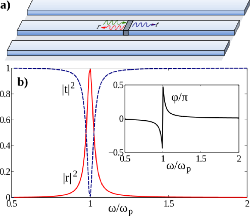
Figure 1: (color online) (a) An open transmission line interrupted by a Josephson junction. (b) Reflection, $r$, transmission, $t$, and phase of the transmitted beam, $\varphi=\arg t$, vs. incoming photon frequency, in units of the plasma frequency $\omega_{p}$. We use $Z_{0}/Z_{J}=10$.

III Quantum circuit crystals

We can scale up the previous results, studying periodic arrangements of junctions both in one and two dimensions. These and other setups Shen et al. (2007); Rakhmanov et al. (2008); Zagoskin et al. (2009); Hutter et al. (2011) can be seen as a generalization of photonic crystals to the quantum microwave regime, with similar capabilities for controlling the propagation of photons: engineered dispersion relations, gaps of forbidden frequencies, localized modes, adjustable group velocities Nation et al. (2009) and index of refraction, and control of the emission and absorption of embedded artificial atoms (i.e. improved cavities) Joannopoulos et al. (2008).

In the following, we will use the linearized scattering theory discussed so far. Regarding possible nonlinear corrections, we expand the cosine term in (1), $1/(2L_{J})\delta\phi^{2}(1-(2\pi)^{2}/(12/\Phi_{0}^{2})\delta\phi^{2})$, containing both the linear contribution and the first nonlinear correction. Since we are working in the single-photon regime, we can replace $\delta\phi^{2}$ by its fluctuations on the vacuum which are proportional to the discontinuity of the wavefunction on that point $\delta\phi\sim\sqrt{\hbar Z_{0}/2}$. All together implies a correction of $0.2\%$ compared to the linear contribution. If we simply view these nonlinear corrections as an inductance dispersion we conclude that we can safely neglect them, since as we will show in section IV.2 such a dispersion hardly affects the transport properties.

III.1 One dimensional circuit crystals

The simplest possible instance of a quantum circuit crystal consists of a unit cell with $N$ junctions that repeat periodically in a one dimensional line. The Lagrangian is a generalization of Eq. (1), combining the junctions together with the intermediate line fields. In the 1D case there are no additional constraints on the flux and at equilibrium $\varphi_{j}^{(0)}=\phi^{(0)}(x)=0$ minimizes the energy [see below Eq. (12)]. The scattering problem is translationally invariant and its eigensolutions are determined by the transfer matrix of the unit cell, $T_{\mathrm{cell}},$ which relates the field at both sides, $\tilde{\phi}_{L,R}(x)=a_{L,R}e^{ikx}+b_{L,R}e^{-ikx},$ through

$$\left(\begin{array}[]{l}a_{R}\\ b_{R}\end{array}\right)=T_{\mathrm{cell}}(\omega)\left(\begin{array}[]{l}a_{L}\\ b_{L}\end{array}\right).$$ (9)

For a setup with junctions and free lines, the transfer matrix has the form $T_{\mathrm{cell}}=\prod_{i=1}^{N}T_{i}D_{i}$, where $T_{i}$ is the transfer matrix of the $i$-th junction and $D_{i}$ is the free propagator through a distance $d_{i}$ Shen et al. (2007)

$$T_{i}=\left(\begin{array}[]{cc}1/t_{i}^{*}&-r_{i}^{*}/t_{i}^{*}\\ -r_{i}/t_{i}&1/t_{i}\end{array}\right),\;D_{i}=\left(\begin{array}[]{cc}e^{i\omega d_{i}/v}&0\\ 0&e^{-i\omega d_{i}/v}\end{array}\right).$$ (10)

The stationary states are given by Bloch waves, which are eigenstates of the displacement operator between equivalent sites. Since this operator is unitary, the eigenvalue can only be a phase, $\phi(x_{j+1})=\exp(ip)\phi(x_{j})$, which we associate with the quasimomentum $p=kd$ with $d$ the intercell distance. Moreover, as any two equivalent points in the lattice are related by the transfer matrix and some free propagators, the result is an homogeneous system of linear equations whose solution is found by imposing $\mathrm{det}[T_{\mathrm{cell}}(\omega)-e^{ip}]=0$ or,

$$2\cos(p)={\rm Tr}[\hat{T}_{\rm cell}(\omega)].$$ (11)

As an example, Fig. 2 shows the dispersion relation $\omega(p)$ for two simple arrangements. The first one is a line with identical Josephson frequency $\omega_{p}$ and impedance $Z_{J}$, evenly spaced a distance $d$ [Fig. 2a]. The second one is also periodic, but the unit cell contains two junctions with different properties, $(\omega_{p},Z_{J})$ and $(\omega_{p}^{\prime},Z_{J}^{\prime})$, which are spread with two different spacings [Fig. 2c]. We find one band gap around $\omega=\omega_{p}$ in the first setup, and two band gaps around $\omega=\omega_{p}$ and $\omega=\omega_{p}^{\prime}$ in the second, more complex case.

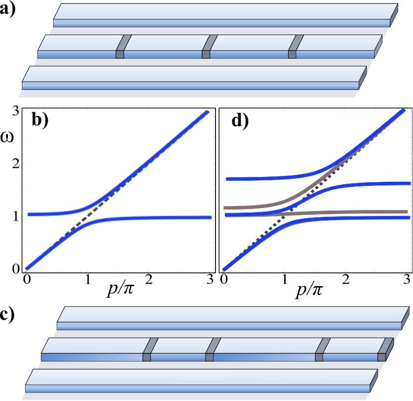
Figure 2: (color online) Photonic crystals with one (a) or two (c) junctions per unit cell and their respective energy bands (b and d) vs. quasimomentum $p$. We use $Z_{0}/Z_{J}=10$ and $d=0.1\lambda_{J}$ with $\lambda_{J}$ the typical wave lenght ($\lambda=2\pi v/\omega_{J}$. In (d) $\omega_{p}^{\prime}/\omega_{p}=0.6$ (blue) or $0.9$ (gray) and and the distance inside the unit cell is $0.01/d$. Notice in (d) that in the lower band the gray and blue line are indistinguishable.

These one dimensional microwave photonic crystals have a variety of applications Joannopoulos et al. (2008). The first one is the suppression of spontaneous emission from qubits, which is achieved by tuning their frequency to lay exactly in the middle of a band gap. Another application is the dynamical control of group velocities. While the width of the band gaps is more directly related to the values of $Z_{J}$ and the separation among scatterers, their position depends on the scatterer frequency, $\omega_{p}$. Replacing the JJs with SQUIDs not ; Haviland2000 ; Hutter et al. (2011), it becomes possible to dynamically tune the slopes of the energy bands, changing from large group velocities (large slope) to almost flat bands (cf. Fig. 2d) where photons may be effectively frozen Shen et al. (2007). Flat bands may themselves be used to create quantum memories and also to induce a tight-binding model on the photons, in the spirit of coupled-cavity systems Hartmann et al. (2006); Angelakis et al. (2007). A third application is the engineering of dissipation where photonic crystals provide a new arena for theoretical and experimental studies. We will focus on this point in the last section, studying the relation between disorder, localization and entanglement generation in 1D quantum circuit crystals.

III.2 Two-dimensional circuit crystals

The evolution from one dimensional arrangements to two-dimensional or quasi-2D circuit crystals demands a careful analysis. The reason for this extra complication is that, unlike in 1D or tree configurations, phase quantization along closed paths introduces new contraints that prevent us from gauging away the static phases $\varphi_{ij}^{(0)}$ and fluxes $\phi^{(0)}(x,y)$ in absence on travelling photons. More precisely, for any closed path $\mathrm{C}$ on the lattice we have

$$\sum_{\rm C}\varphi_{i,j}=2\pi n-\frac{2\pi}{\Phi_{0}}\big{(}\Phi_{\rm ext}+\Phi_{\rm ind}\big{)},\quad n\in\mathbb{Z}$$ (12)

Where $\varphi_{ij}$ are the phase differences along each branch and $\Phi_{\rm ext}+\Phi_{\rm ind}$ is the sum of external and induced fluxes enclosed by $C$. The presence of these fluxes may forbid an equilibrium condition with all phases equal to zero.

The physics of our two-dimensional crystals is intimately related to that of 2D Josephson junction arrays (JJAs), a system whose equilibrium and non-equilibrium properties have been thoroughly studied in the last twenty years Majhofer et al. (1991); Phillips et al. (1993); Domínguez and José (1996); Mazo and Ciria (1996); Newrock et al. (1999); Ciria and Giovannella (1999); Mazo (2002); Mazo and Orlando (2003). In particular, we know that JJAs constitute a physical realizations or the classical frustrated XY model, where frustration is similarly induced by the fluxes threaded through the 2D plaquettes.

A proper study of the photonic excitations must therefore begin by studying the static state on top of which they will propagate. For that we may rely on the classical nonlinear expression for the circuit’s energy, built from capacitive and inductive terms, where the latter contain both the junctions and the (adimensional) mutual inductance matrix, $L_{ij,kl}$ Ciria and Giovannella (1999)

$${\mathcal{V}}=-E_{J}\left[\sum_{i,j}\cos(\varphi_{ij})+\frac{1}{2}\sum_{ij,kl}\sin(\varphi_{ij})L_{ij,kl}\sin(\varphi_{kl})\right].$$ (13)

The optimization of this problem is a formidable task: minimization of (13) subjected at (12) when the induced flux are related to the current (phases) through the inductance matrix. In fact, there is no known solution if any DC field is applied. However, let us focus on a setup without external fields, then $\varphi_{ij}^{(0)}=0$. This is stable against small perturbations and against the quantum fluctuations induced both by the capacitive terms and the travelling photons because the phases are linear in the applied field at small fields Domínguez and José (1996) and they enter on second order in the scattering equations [Cf. Eq. (6)].

Starting from such stable solution $\varphi_{ij}^{(0)}=\phi^{(0)}(x,y)=0$, we can redo the linear scattering theory, which now contains horizontally and vertically propagating fields [Fig. 3],

$$\tilde{\phi}_{ij}^{(h)} = a_{ij}^{(h)}{\rm e}^{ik_{x}x}+b_{ij}^{(h)}{\rm e}^{-ik_{x}x}$$ (14)

$$\tilde{\phi}_{ij}^{(v)} = a_{ij}^{(v)}{\rm e}^{ik_{y}y}+b_{ij}^{(v)}{\rm e}^{-ik_{y}y}$$

with $\textbf{k}=(k_{x},k_{y})$. Pretty much like in the one dimensinal case, invoking periodicity the solutions are Bloch waves,

$$\left(\begin{array}[]{l}a^{(h,v)}_{ij}\\ b^{(h,v)}_{ij}\end{array}\right)=\sum_{\bf p}{\rm e}^{i{\bf p}{\bf u}}\left(\begin{array}[]{l}a_{\bf p}^{(h,v)}\\ b_{\bf p}^{(h,v)}\end{array}\right).\quad{\bf u}=(i,j)$$ (15)

To obtain the condition for the quasimomentum ${\bf k}={\bf p}d$ we relate the fields in ($i,j$) with the ones at ($i-1,j$) and ($i,j-1$) as marked in figure 3. Together with (15) we end up in a homogeneus set of linear equations, see Appendix A for the explicit calculation . When both the horizontal and vertical branches are equivalent, this simplifies to [cf. Eq. (11)]

$$\cos(p_{x})+\cos(p_{y})={\rm Tr}[\hat{T}_{\rm cell}(\omega)]$$ (16)

based on the transfer matrix along one horizontal or vertical branch, $\hat{T}_{\rm cell}(\omega)$, from each elementary plaquette.

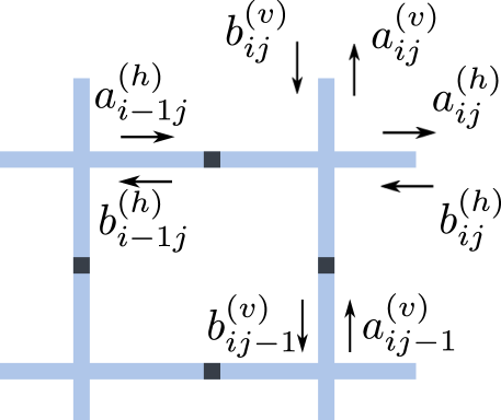
Figure 3: (color online) Scattering variables in the two-dimensional square lattice. Not shown are the intermediate variables: just after the junctions. In Appendix A are denoted with a bar.

III.3 Two-dimensional arrays and negative index of refraction

Once we have the possibility of building two-dimensional circuit crystals, we can also study the propagation of microwaves on extended metamaterials, or on the interface between them, with effects such as evanescent waves (i.e. localized modes) and refraction.

The setup we have in mind is sketched in Fig. 4a, where we draw a two-dimensional array of lines with an interface separating a region with junctions (N) from a region where photons propagate freely (F). We may study how an incoming wave that travels against the boundary enters the N region, inducing reflections, changes of direction and attenuation. For simplicity we will assume that the free region is associated to a vacuum with linear dispersion relation $\omega_{F}^{2}=c_{1}^{2}(k_{x}^{2}+k_{y}^{2})$, where $c_{1}$ the effective velocity of light. The region with junctions, on the other hand, has an engineered dispersion relation $\omega_{N}(k_{x},k_{y})$, as discussed above.

When a wave hits the interface between both regions it may reflect and refract. The wave that penetrates N has to satisfy two constraints: the frequency of the photons must be the same as in F and the component of the wavevector which is parallel to the interface ($p_{y}$ in Fig. 4a) also has to be conserved. Both constraints arise from a trivial matching of the time ($\omega$) and spatial ($p_{y}$) dependence of both waves. Following Ref. Quach et al., 2011 both constraints may be solved by inspecting the dispersion relation in a contour plot [Fig. 4b]. Once the matching values of the momenta are found [red in Fig. 4] the effective group velocities may be computed to determine the trajectory of light. As shown in that plot, in regions where the dispersion relation is convex, the velocity may change orientation and give rise to a refracted angle $\theta_{R}=\arctan(\tan p_{1,y}\cot p_{2,y})$ whose associated index of refraction is negative.

The previous phenomenology has also been proposed for a related platform that consists on a two-dimensional array of coupled atom-cavity systems. Working in the single polariton subspace, it is possible to derive the dispersion relation for those artificial photons Quach et al. (2011) and model the array as an effective photonic material. For a similar band structure and interface as the one shown in Fig. 4, the effective electrical and magnetic permitivity become negative, and one obtains again a negative reffraction angle Veselago (1968). The engineering of these counterintuitive refraction processes is of great interest in the field of linear optics, as negative indices allow designing perfect lenses Pendry (2000), but the propagation of photons in these mixed materials may be interesting also for engineering the dynamics of photon wavepackets, photon routing and 100% efficient qubit-qubit interactions —based on the perfect refocusing properties of these metamaterials.

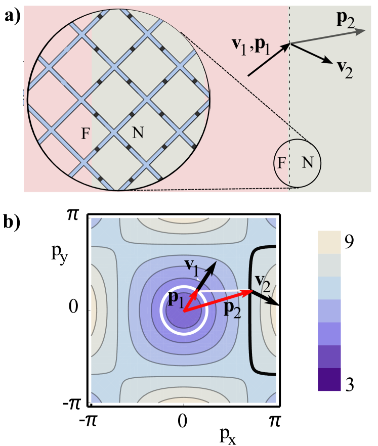
Figure 4: (color online) Two-dimensional circuit crystal. (a) Interface between a junction free region (F) and an engineered bandgap region (N) containing junctions with $\omega_{J}=1.1,\;Z_{0}/Z_{J}=0.8$ and $d=0.1$. Like in the case of polaritons in Ref. Quach et al., 2011 the square lattice must be $\pi/4$-rotated to have negative refraction. (b) Dispersion relations for the region N. In order to find out the refraction angle for wave that propagates from F to N we have to match, on each side of the interface, both the photon frequency and the projection of the wave vector along the boundary, $\mathbf{v}_{1}\cdot\mathbf{e}_{y}=\mathbf{v}_{2}\cdot\mathbf{e}_{y}$. For large enough momenta, (b) shows that the wave gets reversed, that is, the index of refraction is negative.

IV Qubit-Crystal interaction: Quantum Master Equation approach

So far we have discussed lines with junctions for tailoring photonic transport. In this section we study the interaction of these metamaterials with superconducting qubits. Modifying light-matter interaction is a cornerstone in Quantum Optics. One of the most famous examples is the Purcell effect. Confined field enhances or dismisses the spontaneous emission for a quantum emitter. Confinement is usually accomplished by reducing the field to one dimensional waveguides or within cavities or resonators, see e.g. Ref. Cohen-Tannoudji et al., 1992. Related to this is the suppression of spontaneus emission when the transition frequency for the qubit is placed inside the gap of a photonic crystal John and Quang (1994). While the first is at the heart of current circuit QED experiments, the second can be observed with our proposal for engineering band gaps. In this section we modelize such light-matter interaction. In the weak coupling limit we work a quantum master equation and write it in terms of the Green function for the line. The latter can be calculated by knowing the scattering matrix (10). Finally we give a novel application, as the entanglement generation through disorder. To simplify the discussion, and without loss of generality, we focus in the one dimensional case.

Let us write the qubit-line hamiltonian Shen and Fan (2005); Hoi et al. (2011) ,

$$H_{\rm tot}=H_{\rm q}+H_{\rm line}+H_{\rm int},$$ (17)

$H_{\rm q}$ is the qubit Hamiltonian and $H_{line}=\int{\rm d}\omega\omega a^{\dagger}_{\omega}a_{\omega}$ the line expressed in second quantization. The qubit-photons interaction is given by

$$H_{\rm int}=\hbar\sigma^{x}\int{\rm d}\omega g(x,\omega)(a_{\omega}+a_{\omega}^{\dagger})$$ (18)

where $g(x,\omega)$ is the coupling per mode. In Appendix B we show that this coupling can be expressed in terms of the Green function for the line, $G(x,y,\omega)$, as

$$|g(x,\omega)|^{2}=2\pi\,\frac{g^{2}}{v}\,{\rm Im}G(x,x,\omega),$$ (19)

where $v=1/\sqrt{l_{0}c_{0}}$ is the light velocity and $g$ is the coupling in a $\lambda/2$ superconducting resonator with fundamental frequency $\omega$. This is a very convenient way of expressing the qubit-photon interaction because of two reasons. First of all, calculation is simplified to the computation of Green functions, wich in our case is particularly easy, as it can be derived from the the transfer matrix (9) as explained e.g. in Ref. Tai, 1996 [See Appendix app:G for further details] . Second and equally important, the strength of the coupling is parameterized by a simple number, $g$, which corresponds to a measurable quantity in qubit-cavity experiments —ranging from few to hundreds MHz, from strong to ultrastrong coupling regimes.

IV.1 Qubits Quantum Master Equation

Let us introduce a master equation for $N_{q}$ identical qubits placed in the line at positions $x_{j}$. The qubits do not directly interact, but they will do through the line. The qubit Hamiltonian reads,

$$H_{\rm q}=\hbar\,\frac{\epsilon}{2}\,\sum_{j}^{N_{q}}\sigma^{z}_{j}$$ (20)

Interested as we are here in the qubit dynamics, we can trace out the transmission line. Assuming, for simplicity that the weak coupling qubit-line limit holds, one ends up with a master equation for the two qubit reduced density matrix Breuer and Petruccione (2007); Rivas and Huelga (2012)

$$\frac{\partial\varrho}{\partial t}=-\frac{i}{\hbar}[H_{\rm q}+H_{\rm LS},\varrho]-\sum_{i,j=1}^{N_{q}}\gamma_{ij}\left([\sigma_{i}^{+},\sigma_{j}^{-}\varrho]+\mathrm{H.c.}\right).$$ (21)

Here,

$$H_{\rm LS}=\hbar\sum_{ij}^{N_{q}}J_{ij}(\sigma^{+}_{i}\sigma^{-}_{j}+\sigma^{-}_{j}\sigma^{+}_{i})$$ (22)

is the coherent coupling mediated by the line, the so called Lamb shift with,

$$J_{ij}=\frac{g^{2}}{v\epsilon^{2}}{\mathcal{P}}\left[\int{\rm d}\nu\frac{\nu^{2}{\rm Im}G(r_{i},r_{j},\nu)}{\epsilon-\nu}\right]$$ (23)

Finally the rates $\gamma_{ij}$ read,

$$\gamma_{ij}=2\pi\frac{(\hbar g)^{2}}{v}{\rm Im}G(r_{i},r_{j},\epsilon)+\lambda\delta_{ij}$$ (24)

with $\lambda$ the phenomenological non-radiative rate, coming from the intrinsic losses of the qubits, see Appendix B for details.

The simplest situation that is described by this model is that of an open transmission line, with no intermediate scatterers. In this case the line gives rise to both both a coherent and incoherent coupling, quantified by $J_{ij}$ and $\gamma_{ij}$ respectively, which depend on the wavelength of the photons, the qubit separation and their energies. In this case without junctions, $G(x_{i},x_{j},\omega)=i(v/2\omega){\rm e}^{i\omega/v|x_{i}-x_{j}|}$ and thus

$$\gamma_{ij}=(v/2\omega)\cos[\omega/v(x_{i}-x_{j})],$$ (25)

$$J_{ij}=(v/2\omega)\sin[\omega/v(x_{i}-x_{j})].$$

Note how each of these couplings can be set independently set to zero. This has been used for modify the qubits emission going from superradiance and subradiance Gonzalez-Tudela et al. (2011), and it describes recent results in multi-qubit photon scattering van Loo et al. (2012).

IV.2 Entanglement through disorder

With all this theory at hand we move to study a concrete example where we put together structured lines, qubits, disorder and entanglement. So far we discussed regular (periodic) arrangments of junctions producing an ideal photonic crystal. It is feasible to produce them, despite fabrication errors, and the junctions within the same sample are very similar. Nevertheless it can be interesting to induce disorder in the scattering elements, either statically, intervening in the design or deposition processes, or dynamically, replacing the junctions with SQUIDs and dynamically tuning their frequencies. Disorder may have a dramatic influence in the transport properties of the photonic crystal Kaliteevski et al. (2006). On the one hand, the transmission coefficient averaged over an ensemble of random scatterers $\langle T\rangle$ decays exponentially with increasing length $L$ of the disordered media, similar to Anderson’s localization Berry and Klein (1997). On the other hand disorder fights against the interference phenomena that gives rise to the existence of band gaps. The consequence of this competition will be that a sufficiently large disorder could restore the transmission in the frequency range that was originally forbidden John (1987); Yu et al. (1999); Kaliteevski et al. (2006). In what follows we exploit this phenomenon in connection to a purely quantum effect: the entanglement generation through disordered media.

Our model setup consists on two well separated flux qubits, $N_{q}=2$ in (21) and (22), which are coupled by a quantum circuit disordedered media  [Fig. 5]. The qubits will be at their degeneracy points and one of them is driven by an external resonant classical field: $\omega_{\mathrm{d}}=\epsilon$,

$$H_{\rm q}=\frac{\epsilon}{2}(\sigma^{z}_{1}+\sigma^{z}_{2})+f({\rm e}^{-i\omega_{\mathrm{d}}t}\sigma^{+}_{1}+\mathrm{H.c.})\;.$$ (26)

The line, seen now as a quantum bath, has been interrupted by a set of JJ forming the disordered media. The line itself follows our previous scattering theory with uniform disorder $\delta$ in the frequency $\omega_{p}\to\omega_{p}(1+\delta)$ and impedance $Z_{J}\to Z_{J}(1+\delta)$. We use the master equation (21) and compute the coefficients in the case of two qubits separated by disorder as in figure 5. As demonstrated in Appendix C the final expressions read,

$$J_{12}=\gamma_{0}{\rm Im}(T\exp(-ik2D))/2\;,$$ (27)

accounting for the coherent coupling with the cross-dissipation rate

$$\gamma_{12}=\gamma_{0}{\rm Re}(T\exp(-ik2D))\;.$$ (28)

These interactions compete with the individual decay rates of the qubits,

$$\gamma_{ii}=\gamma_{0}(1-{\rm Re}(R\exp(-ikD)))+\lambda\;,$$ (29)

which includes a phenomenological non-radiative decay channel, $\lambda$ coming from the intrinsic losses of the qubits [Cf. Eq. (24)]. In all these formulas appear the effective rate $\gamma_{0}=\pi\hbar^{2}g^{2}/vk$, the total transmission and reflection $T$ and $R$ at the boundaries of the disordered part, and the qubit-disorder separation, $D$. In figure 5 this dependence dissapears since the results are drawn at the distance $D$ that maximizes the concurrence.

The physical picture that results is intuitively appealing: for the qubits to be entangled, the noisy environment should be able to transmit photons, $T\neq 0$, as both the coherent and incoherent couplings depend on it. Moreover, all photons which are not transmitted but reflected add up to the ordinary spontaneous emission rates of the qubits, $\gamma_{ii}$. And finally, for a wide parameter range the two qubits are entangled also at $t\to\infty,$ in the stationary state of the combined system, $\partial_{t}\varrho_{\rm stationary}=0$. We have quantified the asymptotic amount of entanglement using the concurrence, $C$, for a variety of disorder intensities in a medium which is composed of $N=20$ junctions which are uniformly spread over a distance $L=2\lambda$. Fig. 5 shows the result of averaging 500 realizations of disorder and contains the two ingredients stated above. We observe that for zero or little disorder entanglement becomes zero at the band gap, $\omega/\omega_{p}=1$, where photons are forbidden due to interference. However, as we increase disorder the gap vanishes and entanglement enters the region around it. Outside the gap the effect is the opposite: disorder reduces the amount of entanglement, as it hinders the transmission of photons. To understand the modulations of the plot one must simply realize that the value of $C$ mostly depends on the ratio between $\gamma_{12}$ and $\gamma_{ii}$ Gonzalez-Tudela et al. (2011), and these are complex functions of $T$ and $R$, respectively Chang et al. (2011).

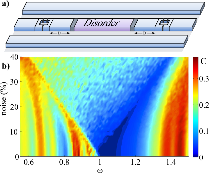
Figure 5: (color online) (a) Two qubits connected by a noisy environment. (b) Concurrence between the qubits for model (21) as a function of frequency and fabrication error ($\delta$). We simulated a setup with 20 junctions regularly spaced over a distance $L=2\lambda$, averaging over 500 realizations. We use the parameters, $Z_{0}/Z_{J}=10$, $\epsilon=\omega_{d}$, $\lambda=0.4\gamma_{0}$ and $f=0.1\gamma_{0}$.

V Conclusions and outlook

In this work we have developed an architecture for quantum metamaterials based the scattering of travelling photons through Josephson junctions. We have shown that a single junction acts as a perfect mirror for photons that resonate with its plasma frequency. Using the scaterring matrix formalism, we have studied the band structure of networks of transmission lines with embedded junctions. We demonstrate that these setups behave as quantum metamaterials that can be used to control the propagation of individual photons. This opens the door to the usual applications of classical metamaterials, such as cloaking or subwavelength precision lenses. In particular, as an illustration of the formalism for two-dimensional networks, we discussed the observation of a negative index of refraction.

We want to remark that the utility of junction quantum metamaterials extends beyond the classical regime, with interesting applications in the fields of quantum information and quantum circuits. Replacing individual junctions with tunable SQUIDs opens the door to the dynamical control of band gaps, or the generation of flat bands, which is useful for stoping light, implementing quantum memories and what would be the equivalent of coupled cavities arrays.

Two important applications of this tunability are engineering of disorder and dissipation. In the first case the focus is on the photons that travel through the network, while in the second case the focus is on how this network acts on few-level systems that are embedded in them. We combine both approaches by developing the theory for multi-qubit interactions in a quantum metamaterial. The resulting master-equation formalism combines the effects of spontaneous emission in the artificial material, with the interaction mediated by the exchange of photons. We show that two competing effects —Anderson localization suppresses transport, but disorder populates the band gaps with localized states—, lead to the generation of stationary entanglement in these setups.

We strongly believe that this architecture is within reach for the experimental state of the art. Building on very simple components, it offers a great potential both for quantum information with flying microwave qubits (photons), and for the static and dynamic control of stationary qubits. In the near future we wish to explore the application of this technology as a replacement for the coupled-cavity architecture, where the one- or two-dimensional network replaces the cavities, offering new possibilities of tunability and variable geometry.

Finally, we want to remark that shortly after the rewrite of this manuscript, a related work appeared that develops a similar formalism for Josephson junctions embedded in transmission lines Bourassa et al. .

Appendix A Transfer Matrix in the 2D case

We detail here the calculations needed to obtain condition (16) in the main text. The idea is to relate the horizontal and vertical fields (14) on both sides of each junction, as shown in Fig. 3. Introducing the vectors

$$\mathbf{w}^{(h,v)}_{\bf d}=\left(\begin{array}[]{c}a_{\bf d}^{(h,v)}\\ b_{\bf d}^{(h,v)}\end{array}\right)\;,$$ (30)

the fields at both sides of the junction are related, see Eq. (9),

$$\bar{\mathbf{w}}_{ij}^{(h)} =T^{(h)}_{\rm cell}(\omega)\mathbf{w}_{i-1j}^{(h)},\;$$ (31)

$$\bar{\mathbf{w}}_{ij}^{(v)} =T^{(v)}_{\rm cell}(\omega)\mathbf{w}_{ij-1}^{(v)},\;$$ (32)

Finally we get the final $\mathbf{w}_{ij}^{(h,v)}$ by resorting to continuity and current conservation in the corner. It is convenient then to define the vectors $\mathbf{e}_{\pm}^{t}=(1,\pm 1)$. Using this notation, the continuity condition is written as follows

$$\mathbf{e}_{+}^{t}T^{(h)}_{\rm cell}\mathbf{w}_{i-1j}^{(h)}=\mathbf{e}_{+}^{t}T^{(v)}_{\rm cell}\mathbf{w}_{ij-1}^{(v)}=\mathbf{e}_{+}^{t}\mathbf{w}_{ij}^{(h)}=\mathbf{e}_{+}^{t}\mathbf{w}_{ij}^{(v)},$$ (33)

and current conservation at the corners reads

$$\mathbf{e}_{-}^{t}T^{(v)}_{\rm cell}\mathbf{w}_{i-1j}^{(h)}+\mathbf{e}_{-}^{t}T^{(h)}_{\rm cell}\mathbf{w}_{ij-1}^{(v)}=\mathbf{e}_{-}^{t}\mathbf{w}_{ij}^{(h)}+\mathbf{e}_{-}^{t}\mathbf{w}_{ij}^{(v)}.$$ (34)

writting now $\mathbf{w}_{ij}^{(h,v)}$ as Bloch waves (15) we end up 4-coupled homogeneus set of linear equations:

$${\mathbb{M}}(\omega)\left(\begin{array}[]{c}\mathbf{e}_{+}^{t}\mathbf{w}_{\bf p}^{(h)}\\ \mathbf{e}_{-}^{t}\mathbf{w}_{\bf p}^{(h)}\\ \mathbf{e}_{+}^{t}\mathbf{w}_{\bf p}^{(v)}\\ \mathbf{e}_{-}^{t}\mathbf{w}_{\bf p}^{(v)}\end{array}\right)=0$$ (35)

with,

$${\mathbb{M}}(\omega)=\left(\begin{array}[]{cccc}1&0&-1&0\\ 1-{\rm e}^{-ik_{x}}\mathbf{e}_{+}^{t}T_{\rm cell}^{(h)}\mathbf{e}_{+}&-{\rm e}^{-ik_{x}}\mathbf{e}_{+}^{t}T_{\rm cell}^{(h)}\mathbf{e}_{-}&0&0\\ 1&0&-{\rm e}^{-ik_{y}}\mathbf{e}_{+}^{t}T_{\rm cell}^{(v)}\mathbf{e}_{+}&-{\rm e}^{-ik_{y}}\mathbf{e}_{+}^{t}T_{\rm cell}^{(v)}\mathbf{e}_{-}\\ 1-{\rm e}^{-ik_{x}}\mathbf{e}_{-}^{t}T_{\rm cell}^{(h)}\mathbf{e}_{+}&1-{\rm e}^{-ik_{x}}\mathbf{e}_{-}^{t}T_{\rm cell}^{(h)}\mathbf{e}_{-}&{\rm e}^{-ik_{y}}\mathbf{e}_{-}^{t}T_{\rm cell}^{(v)}\mathbf{e}_{+}&1-{\rm e}^{-ik_{y}}\mathbf{e}_{-}^{t}T_{\rm cell}^{(v)}\mathbf{e}_{-}\end{array}\right)$$ (36)

together with the relations due to the scattering matrix (10) properties,

$$(\mathbf{e}_{+}^{t}T_{\rm cell}^{(h,v)}\mathbf{e}_{+})(\mathbf{e}_{-}^{t}T_{\rm cell}^{(h,v)}\mathbf{e}_{-})-(\mathbf{e}_{+}^{t}T_{\rm cell}^{(h,v)}\mathbf{e}_{-})(\mathbf{e}_{-}^{t}T_{\rm cell}^{(h,v)}\mathbf{e}_{+}) =1$$ (37)

$$(\mathbf{e}_{+}^{t}T_{\rm cell}^{(h,v)}\mathbf{e}_{+})+(\mathbf{e}_{-}^{t}T_{\rm cell}^{(h,v)}\mathbf{e}_{-})={\rm Tr}[T_{\rm cell}^{(h,v)}]$$ (38)

Putting alltogether we have that ${\rm det}[{\mathbb{M}}]=0$ yields the generalized condition for the two-dimensional case. In the simplest case of fully symmetric configuration: $T_{\rm cell}^{(h)}=T_{\rm cell}^{(v)}:=T_{\rm cell}$ we simply have [Cf. Eq. (11)],

$$\cos(p_{x})+\cos(p_{y})={\rm Tr}[T_{\rm cell}(\omega)]$$ (39)

Appendix B Modelling qubit-line interaction and Master Equation

In this appendix we develop the model for the qubit-line interaction. We will focus on flux qubits for the sake of concreteness, but the results are analogous for other qubits. Besides we will discuss the master equation governing the qubits dynamics. Finally we rewrite the formulas in terms of the Green function.

For flux qubits the coupling is inductive and can be written in circuit and/or magnetic language as,

$$H_{\rm int}=MI_{\rm qubit}\times I_{\rm line}=\mu B\;,$$ (40)

here $M$ stands for the mutual inductance, $I_{\rm qubit}$ and $I_{\rm line}$ are the currents and $\mu$ is the magnetic qubit dipole, while $B$ is the magnetic field generated in the cavity.

The current in the line is given by $I_{\rm line}=\frac{1}{l_{0}}\partial_{x}\phi(x)$. We will expand this field using normal modes, $u_{n}(x)$, following the usual quantization $\phi(x,t)=\sum u_{k}(x)q_{k}(t)$, but imposing that $u_{k}$ are dimensionless Bourassa et al. (2009) and satisfy the orthonormality condition $\int c_{0}u_{k}\;u_{l}{\rm d}x=C_{r}\delta_{kl}$ with the average capacitance $C_{r}:=\int c_{0}{\rm d}x$. Expressing the canonical operator $q_{k}$ in the Fock basis $q_{k}=(a^{\dagger}_{k}+a_{k})\sqrt{\hbar/2\omega_{n}C_{r}}$ gives us the final expression

$$I_{\rm line}=\frac{1}{l_{0}}\sum\sqrt{\frac{\hbar}{2\omega_{k}C_{r}}}\partial_{x}u_{k}(x)(a_{k}^{\dagger}+a_{k})\;.$$ (41)

The magnetic field-current relation is given by $B_{\rm line}=\mu_{0}I_{\rm line}/\pi d$, with $d$ the distance between plates in the coplanar wave-guide. The quantized magnetic dipole for the qubit can also be expressed in terms of the qubit area, $A$ and the stationary current $I_{p}$ as $\mu=I_{p}A\sigma^{x}$. Putting alltogether we find the interaction Hamiltonian (40)

$$H_{\rm int}=I_{p}A\frac{\mu_{0}}{\pi d}\frac{1}{l_{0}}\frac{\hbar}{2C_{r}}\;\sigma_{x}\;\sum\frac{1}{\sqrt{\omega_{k}}}\partial_{x}u_{k}(x)(a_{k}^{\dagger}+a_{k})\;.$$ (42)

We can introduce the coupling strenght per mode with frequency $\omega_{0}$ Lindström et al. (2007),

$$\hbar g=I_{p}A\frac{\mu_{0}}{\pi^{3/2}d}\omega_{0}\sqrt{\frac{1}{\hbar Z_{0}}}$$ (43)

Grouping the constants and using the expression for $g$, Eq. (43), we rewrite (42),

$$H_{\rm int}=\hbar\frac{g}{\omega_{0}}v^{3/2}\frac{\pi}{\sqrt{2L}}\;\sigma_{x}\;\sum\frac{1}{\sqrt{\omega_{k}}}\partial_{x}u_{k}(x)(a_{k}^{\dagger}+a_{k})$$ (44)

where $v=1/\sqrt{l_{0}c_{0}}$ the light velocity in the line and $\omega_{0}$ the fundamental frequency of a cavity with a given $g$ and $L$ is the Lenght. As expected the above expression is nothing but the spin boson model.

B.1 Green Function formalism

It turns out useful to rewrite (44) in terms of the Green Function for the line. We begin the discussion by recalling the field wave equation. Equivalently to layered photonic crystals, it is sufficient to work the case of homogeneous line, since the problem we are dealing with is piecewise homogeneousNovotny and Hecht (2006). For flux qubits the coupling is through the line current [cf. Eq. (40)]. Thus it is more convenient to discuss the wave equation for the mode derivatives

$$\frac{1}{l_{0}}\partial^{2}_{x}(\partial_{x}u_{k})=-\omega_{n}^{2}c_{0}\partial_{x}u_{k}$$ (45)

with the orthogonality condition,

$$\int{\rm d}x\partial_{x}u_{k}\partial_{x}u_{k^{\prime}}=Lk^{2}\delta_{kk^{\prime}}.$$ (46)

The Green function for this Sturm-Liouville problem reads

$$\partial_{x}^{2}G(x,x^{\prime},\omega)+\frac{\omega^{2}}{v^{2}}G(x,x^{\prime},\omega)=-\delta(x-x^{\prime}).$$ (47)

It is pivotal the relation [cf. Eq. (8.114) in Ref. Novotny and Hecht, 2006]

$${\rm Im}G(x,x^{\prime},\omega)=\frac{v^{4}}{L}\frac{\pi}{2}\sum_{k}\frac{\partial_{x}u_{k}(x)\partial_{x}u_{k}^{*}(x^{\prime})}{\omega_{k}^{3}}\delta(\omega-\omega_{k})\;.$$ (48)

By rewriting (44) in the continuum limit,

$$H_{\rm int}=\hbar\sigma^{x}\int{\rm d}\omega g(x,\omega)(a_{\omega}+a_{\omega}^{\dagger})$$ (49)

with $g(x,\omega)$ [combining (48), (44) and (49)]

$$|g(x,\omega)|^{2}=2\pi\,\frac{g^{2}}{v}\,{\rm Im}G(x,x,\omega)\;,$$ (50)

i.e. equations (18), (19) in the main text.

B.2 Quantum Master Equation

Setting the temperature to zero (typical experiments are at the mK while frequencies are GHz) the qubit dynamics, after integrating the bosonic modes, is given by the standard master equation in Linblad form wich assumes weak coupling between the line and the qubit Breuer and Petruccione (2007); Rivas and Huelga (2012),

$$\partial_{t}\rho= -\frac{i}{\hbar}[H_{\rm qubit}+H_{\rm LS},\rho]$$ (51)

$$+\sum_{i,j}\Gamma_{i,j}\left(\sigma^{-}_{i}\rho\sigma^{+}_{j}-\frac{1}{2}\{\sigma^{+}_{i}\sigma^{-}_{j}\rho\}\right)$$

$$+\lambda\sum_{i,j}\left(\sigma^{-}_{i}\rho\sigma^{+}_{j}-\frac{1}{2}\{\sigma^{+}_{i}\sigma^{-}_{j}\rho\}\right)$$

where $\{,\}$ is the anticonmutator. In the equation we have distinguished the contribution to the decay rates coming from the qubit-line coupling, $\Gamma_{ij}$, from other noise sources affecting the qubits, denoted with a phenomenological strenght $\lambda$. The explicit expressions for the $\Gamma_{i,j}$ are e.g. Breuer and Petruccione (2007); Rivas and Huelga (2012)

$$\Gamma_{i,j}=|g(\epsilon)|^{2}$$ (52)

Finally, we also have to consider the Lamb Shift

$$H_{\rm LS}=\sum J_{ij}\left(\sigma_{i}^{+}\sigma_{j}^{-}+\sigma_{j}^{+}\sigma_{i}^{-}\right)$$ (53)

with

$$J_{ij}=\frac{1}{2\pi\omega^{2}}{\mathcal{P}}\left[\int{\rm d}\nu\frac{\nu^{2}{\rm Im}|g(\nu)|^{2}}{\epsilon-\nu}\right]$$ (54)

where $\mathcal{P}[\;]$ means principal value integral.

By defining,

$$\gamma_{ij}=\Gamma_{ij}+\lambda\delta_{ij}$$ (55)

together with (50) we get coefficients (23) and (24) in the main text.

Appendix C Green Function for an arrangement of scatterers

In the following we find $G(x_{i},x_{j},\omega)$ for the problem discussed in the main text. We show that $G(x_{i},x_{j},\omega)$ is written in terms of reflection and transmission coefficients, $R$ and $T$ respectively. We use this to express the decays and cross couplings, $\gamma_{ij}$ and $J_{12}$, in terms of the scattering parameters, making explicit the connection between the photonic transport in the line and the dynamics for the qubits coupled to it.

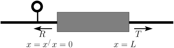
Figure 6: Sketch for the Green function calculation. The “black box” is characterized by transmission and reflection coefficientes. The source (Dirac Delta) is represented by the ring attached to the line.

In our case, two qubits placed at possitions $x_{1}$ and $x_{2}$ with a set of junctions in between (see figure 6) $G(x_{i},x_{j},\omega)$ can be computed as follows. The equation for the Green function (47) is a field equation with a source (because of the Dirac delta) at $x=x^{\prime}$. The junctions cover the region from $x=0$ to $x=L$, therefore $x_{1}<0$ and $x_{2}>L$. This situation is analogous to have a boundary with reflection $R$ and transmission $T$, as despicted in figure 6. In this situation the Green Function is given by [Eqs. (2.34) and (2.35) in Tai (1996)],

$$G(x,x^{\prime},\omega)=\left\{\begin{array}[]{ll}\frac{i}{2k}\left({\rm e}^{-ik(x-x^{\prime})}-R{\rm e}^{-ik(x+x^{\prime})}\right)&x<x^{\prime}\\ \frac{i}{2k}\left({\rm e}^{ik(x-x^{\prime})}-R{\rm e}^{-ik(x+x^{\prime})}\right)&x^{\prime}<x<0\\ \frac{i}{2k}T{\rm e}^{ik(x-(x^{\prime}+L))}&x>L\end{array}\right.$$ (59)

We remind that the minus sign in front of the $R$ above comes because the Green function in (48) is given in terms of $\partial_{x}u_{k}$.

Finally, the coefficients in the master equation read [Cf. Eqs. (24) and (23)]

$$\Gamma_{jj}(\omega_{\rm qubit}) =2\pi\frac{(\hbar g)^{2}}{v}{\rm Im}G(r_{j},r_{j},\omega_{\rm qbuit})$$

$$=2\pi\frac{(\hbar g)^{2}}{v}\frac{1}{2k}\Big{(}1+{\rm Re}(R)\Big{)}$$ (60)

$$\Gamma_{12}(\omega_{\rm qubit}) =2\pi\frac{(\hbar g)^{2}}{v}{\rm Im}G(r_{1},r_{2},\omega_{\rm qbuit})$$

$$=2\pi\frac{(\hbar g)^{2}}{v}\frac{1}{2k}{\rm Re}(T{\rm e}^{-ik(x_{1}-x_{2})})$$ (61)

The last obstacle to write the master equation is to perform the integral in (23). Here we made use of the so called Generalized Kramers-Kroning relation Dzsotjan et al. (2011), namely

$${\mathcal{P}}\left[\int_{0}^{\infty}\;{\rm d}\omega\frac{\omega^{2}}{v^{2}}\frac{{\rm Im}G(r_{j},r_{k},\omega)}{\omega-\omega_{\rm qubit}}\right]=\frac{\pi}{2}\frac{\omega_{\rm qubit}^{2}}{v^{2}}{\rm Re}G(r_{j},r_{k},\omega)$$ (62)

Thus,

$$J_{12}=\pi\frac{(\hbar g)^{2}}{v}\frac{1}{2k}{\rm Im}(T{\rm e}^{-ik(x_{1}-x_{2})})$$ (63)

Introducing the definition,

$$\gamma_{0}=\pi\frac{(\hbar g)^{2}}{v}\frac{1}{k}$$ (64)

we end up with the expressions used in the main text.

References

- You and Nori (2011) J. Q. You and F. Nori, Nature (London) 474, 589 (2011).
- Wallraff et al. (2004) A. Wallraff, D. I. Schuster, A. Blais, L. Frunzio, R.-S. Huang, J. Majer, S. Kumar, S. M. Girvin, and R. J. Schoelkopf, Nature 431, 162 (2004).
- Hofheinz et al. (2009) M. Hofheinz, H. Wang, M. Ansmann, R. C. Bialczak, E. Lucero, M. Neeley, A. D. O’Connell, D. Sank, J. Wenner, J. M. Martinis, et al., Nature 459, 546 (2009).
- Majer et al. (2007) J. Majer, J. M. Chow, J. M. Gambetta, J. Koch, B. R. Johnson, J. A. Schreier, L. Frunzio, D. I. Schuster, A. A. Houck, A. Wallraff, et al., Nature (London) 449, 443 (2007).
- Dicarlo et al. (2009) L. Dicarlo, J. M. Chow, J. M. Gambetta, L. S. Bishop, B. R. Johnson, D. I. Schuster, J. Majer, A. Blais, L. Frunzio, S. M. Girvin, et al., Nature 460, 240 (2009).
- Ansmann et al. (2009) M. Ansmann, H. Wang, R. C. Bialczak, M. Hofheinz, E. Lucero, M. Neeley, A. D. O’Connell, D. Sank, M. Weides, J. Wenner, et al., Nature 461, 504 (2009).
- Shen et al. (2007) J. T. Shen, M. L. Povinelli, S. Sandhu, and S. Fan, Phys. Rev. B 75, 035320 (2007).
- Rakhmanov et al. (2008) A. L. Rakhmanov, A. M. Zagoskin, S. Savel’ev, and F. Nori, Phys. Rev. B 77, 144507 (2008).
- Zagoskin et al. (2009) A. M. Zagoskin, A. L. Rakhmanov, S. Savel’ev, and F. Nori, physica status solidi (b) 246, 955 (2009).
- (10) Liao, J.-Q., Gong, Z.-R, Zhou, L., Liu, X.-Y., Sun, C.-P., and Nori, F. Phys. Rev. A., 81, 042304 (2010)
- Hutter et al. (2011) C. Hutter, E. A. Tholén, K. Stannigel, J. Lidmar, and D. B. Haviland, Phys. Rev. B 83, 014511 (2011).
- Shen and Fan (2005) J.-T. Shen and S. Fan, Phys. Rev. Lett. 95, 213001 (2005).
- (13) Zhou., L, Gong, Z.-R., Liu, X.-Y., Sun, C.-P., and Nori, F. Phys. Rev. Lett, 101, 100501 (2008)
- (14) Zhou., L, Gong, Z.-R., Liu, X.-Y., Sun, C.-P., and Nori, F. Phys. Rev. A, 78, 063827 (2008)
- Astafiev et al. (2010a) O. Astafiev, A. M. Zagoskin, A. A. Abdumalikov, Y. Pashkin, T. Yamamoto, K. Inomata, Y. Nakamura, and J. S. Tsai, Science 327, 840 (2010a).
- Hoi et al. (2011) I.-C. Hoi, C. M. Wilson, G. Johansson, T. Palomaki, B. Peropadre, and P. Delsing, Phys. Rev. Lett. 107, 073601 (2011).
- Astafiev et al. (2010b) O. V. Astafiev, A. A. Abdumalikov, A. M. Zagoskin, Yu, Y. Nakamura, and J. S. Tsai, Phys. Rev. Lett. 104, 183603 (2010b).
- Romero et al. (2009) G. Romero, J. J. García-Ripoll, and E. Solano, Phys. Rev. Lett. 102, 173602 (2009).
- Peropadre et al. (2011) B. Peropadre, G. Romero, G. Johansson, C. M. Wilson, E. Solano, and J. J. García-Ripoll, Phys. Rev. A 84, 063834 (2011).
- (20) Chen, Y.-F., Hover, D., Sendelbach, S., Maurer, L., Merkel, S., Pritchett, E., Wilhelm, F., and McDermott, R., Phys. Rev. Lett., 108, 217401 (2011)
- Savel’ev et al. (2005) S. Savel’ev, A. L. Rakhmanov, and F. Nori, Phys. Rev. Lett. 94, 157004 (2005).
- Savel’ev et al. (2006) S. Savel’ev, A. L. Rakhmanov, and F. Nori, Phys. Rev. B 74, 184512 (2006).
- Savel’ev et al. (2010) S. Savel’ev, V. A. Yampol’skii, A. L. Rakhmanov, and F. Nori, Reports on Progress in Physics 73, 026501 (2010).
- Makhlin et al. (2001) Y. Makhlin, G. Schön, and A. Shnirman, Rev. Mod. Phys. 73, 357 (2001).
- (25) M. A. Castellanos-Beltran, Irwin, K. D., Hilton, G. C., L. Vale and Lehnert, K. W Nature Physics 4, 928 (2008)
- Wilson et al. (2011) C. M. Wilson, G. Johansson, A. Pourkabirian, J. R. Johansson, T. Duty, F. Nori, and P. Delsing, Nature 479, 376 (2011).
- Niemczyk et al. (2010) T. Niemczyk, F. Deppe, H. Huebl, E. P. Menzel, F. Hocke, M. J. Schwarz, J. J. Garcia-Ripoll, D. Zueco, T. Hummer, E. Solano, et al., Nature Physics 6, 772 (2010).
- Forn-Díaz et al. (2010) P. Forn-Díaz, J. Lisenfeld, D. Marcos, J. J. García-Ripoll, E. Solano, C. J. P. M. Harmans, and J. E. Mooij, Phys. Rev. Lett. 105, 237001 (2010).
- Ong et al. (2011) F. R. Ong, M. Boissonneault, F. Mallet, A. Palacios-Laloy, A. Dewes, A. C. Doherty, A. Blais, P. Bertet, D. Vion, and D. Esteve, Phys. Rev. Lett. 106, 167002 (2011).
- Nation et al. (2009) P. D. Nation, M. P. Blencowe, A. J. Rimberg, and E. Buks, Phys. Rev. Lett. 103, 087004 (2009).
- Bourassa et al. (2009) J. Bourassa, J. M. Gambetta, A. A. Abdumalikov, O. Astafiev, Y. Nakamura, and A. Blais, Phys. Rev. A 80, 032109 (2009).
- Devoret (1995) M. H. Devoret, Les Houches Session LXIII, Quantum Fluctuations pp. 351–386 (1995).
- Joannopoulos et al. (2008) J. Joannopoulos, S. Johnson, J. Winn, and R. Meade, Photonic Crystals: Molding the Flow of Light (Princenton, 2008), 2nd ed.
- (34) When neglecting the self-inductance, A DC SQUID behaves as a single junction with a critical current given by with the magnetic flux across the squid loop.
- (35) D. B. Haviland, K. Andersson and P. Ågren, J. Low. Temp. Phys. 118, 733 (2000)
- Hartmann et al. (2006) M. J. Hartmann, F. G. S. L. Brandão, and M. B. Plenio, Nature Physics 2, 849 (2006).
- Angelakis et al. (2007) D. G. Angelakis, M. F. Santos, and S. Bose, Phys. Rev. A 76, 031805 (2007).
- Majhofer et al. (1991) A. Majhofer, T. Wolf, and W. Dieterich, Phys. Rev. B 44, 9634 (1991).
- Phillips et al. (1993) J. R. Phillips, H. S. J. van der Zant, J. White, and T. P. Orlando, Phys. Rev. B 47, 5219 (1993).
- Domínguez and José (1996) D. Domínguez and J. V. José, Phys. Rev. B 53, 11692 (1996).
- Mazo and Ciria (1996) J. J. Mazo and J. C. Ciria, Phys. Rev. B 54, 16068 (1996).
- Newrock et al. (1999) R. S. Newrock, C. J. Lobb, U. Geigenmüller, and M. Octavio, The Two-Dimensional Physics of Josephson Junction Arrays, vol. 54 of Solid State Physics (Academic Press, 1999).
- Ciria and Giovannella (1999) J. C. Ciria and C. Giovannella, Journal of Physics: Condensed Matter 11, R361 (1999).
- Mazo (2002) J. J. Mazo, Phys. Rev. Lett. 89, 89234101 (2002).
- Mazo and Orlando (2003) J. J. Mazo and T. P. Orlando, Chaos 13, 733 (2003).
- Quach et al. (2011) J. Q. Quach, C.-H. Su, A. M. Martin, A. D. Greentree, and L. C. L. Hollenberg, Optics Express 19, 11018 (2011).
- Veselago (1968) V. G. Veselago, Sov. Phys. Usp. 10, 509 (1968).
- Pendry (2000) J. B. Pendry, Phys. Rev. Lett. 85, 3966 (2000).
- Cohen-Tannoudji et al. (1992) C. Cohen-Tannoudji, J. Dupont-Roc, and G. Grynberg, Atom-Photon Interactions: Basic Processes and Applications (Wiley-Interscience, 1992), ISBN 0471625566.
- John and Quang (1994) S. John and T. Quang, Phys. Rev. A 50, 1764 (1994).
- Tai (1996) C.-T. Tai, Dyadic Green Functions in Electromagnetic Theory (Ieee-Oup Series on Electromagnetic Wave Theory) (Oxford University Press, USA, 1996), 2nd ed.
- Breuer and Petruccione (2007) H.-P. Breuer and F. Petruccione, The Theory of Open Quantum Systems (Oxford University Press, USA, 2007).
- Rivas and Huelga (2012) A. Rivas and S. F. Huelga, Open Quantum Systems An Introduction (Springer, Heidelberg, 2012).
- Gonzalez-Tudela et al. (2011) A. Gonzalez-Tudela, D. Martin-Cano, E. Moreno, L. Martin-Moreno, C. Tejedor, and F. J. Garcia-Vidal, Phys. Rev. Lett. 106, 020501 (2011).
- van Loo et al. (2012) A. F. van Loo, A. Fedorov, K. Lalumière, B. C. Sanders, A. Blais, and A. Wallraff, in APS Meeting Abstracts (2012), p. 29005.
- Kaliteevski et al. (2006) M. A. Kaliteevski, D. M. Beggs, S. Brand, R. A. Abram, and V. V. Nikolaev, Phys. Rev. B 73, 033106 (2006).
- Berry and Klein (1997) M. V. Berry and S. Klein, Eur. J. Phys. 18, 222 (1997).
- John (1987) S. John, Phys. Rev. Lett. 58, 2486 (1987).
- Yu et al. (1999) Yu, M. A. Kaliteevski, and V. V. Nikolaev, Phys. Rev. B 60, 1555 (1999).
- Chang et al. (2011) Y. Chang, Z. R. Gong, and C. P. Sun, Phys. Rev. A 83, 013825 (2011).
- (61) J. Bourassa, F. Beaudoin, J. M. Gambetta, and A. Blais, arXiv:1204.2237.
- Lindström et al. (2007) T. Lindström, C. H. Webster, J. E. Healey, M. S. Colclough, C. M. Muirhead, and A. Y. Tzalenchuk, Superconductor Science and Technology 20, 814 (2007).
- Novotny and Hecht (2006) L. Novotny and B. Hecht, Principles of Nano-Optics (Cambridge University Press, 2006).
- Dzsotjan et al. (2011) D. Dzsotjan, J. Kästel, and M. Fleischhauer, Phys. Rev. B 84, 075419 (2011).