Chiral Y-junction of Luttinger liquid wires at weak coupling: lines of stable fixed points

Abstract

We calculate the conductances of a Y-junction set-up of Luttinger liquid wires threaded by a magnetic flux, allowing for different interaction strength $g_{3}\neq g$ in the third wire. The scattering matrix and the matrix of conductances are parametrized by three variables. For these we derive coupled RG equations, up to second order in the interaction, within the scattering state formalism. The fixed point structure of these equations is analyzed in detail. For repulsive interaction ($g,g_{3}>0$) there is only one stable fixed point, corresponding to the complete separation of the wires. For attractive interaction ($g<0$ and/or $g_{3}<0$) four fixed points are found, whose stability depends on the interaction strength. For special values of the interaction parameters (a) $g=0$, $g_{3}<0$ or (b) $g_{3}+g^{2}/2=0$ and $g<0$ we find whole lines of stable fixed points. We conjecture that lines of fixed points appear generically at interfaces in interaction coupling constant space separating two regions with different stable fixed points. We also find that in certain regions of the $g$–$g_{3}$-plane the RG flow is towards a fixed point without chirality, implying that the effect of the magnetic flux is completely screened.

Introduction. Electron transport in strictly onedimensional quantum wires is governed by the Coulomb interaction between electrons, found to destroy the Landau quasiparticle concept valid in higher dimensions. An important part of that physics is captured by the exactly solvable Tomonaga-Luttinger liquid (TLL) model, in which backward scattering is neglected.Giamarchi (2003) As is well known, transport through junctions of TLL wires is strongly affected by the interaction in the wires, sometimes leading to a complete blocking of transmission.  Many of the early works on the problem of two TLL-wires connected by a junction employed the method of bosonization Kane and Fisher (1992); Furusaki and Nagaosa (1993), or, for special values of the interaction parameter, used a mapping on to exactly solvable modelsWeiss et al. (1995); Fendley et al. (1995). An alternative formulation using the fermionic representation has been pioneered by Yue et al. (1994). There the renormalization group (RG) method has been used. The advantage of the latter formulation is that it is rather flexible, allowing for the inclusion of spin, of backward scattering, the study of wires with two impurities Polyakov and Gornyi (2003), and of multi-lead junctionsDas et al. (2004); Lal et al. (2002) in and out of equilibrium. The limitation of the original model calculation Yue et al. (1994) to weak coupling has prevented a more widely spread use of this method. It may be shown, however, that the method may be extended to apply in the strong coupling regime as well, by summing up an infinite class of leading contributions in perturbation theoryAristov and Wölfle (2009). Quite generally, the transport behavior at low energy/temperature is dominated by only a few fixed points of the RG flow. The most common and intuitively plausible fixed points are those with quantized conduction values, $G=0,1$, in units of the conductance quantum $G_{0}=e^{2}/h$. There may, however, appear additional fixed points associated with noninteger conductance values. A particularly interesting case is that of a symmetric three-lead junction with broken chiral symmetry, as induced by a magnetic flux threading the junction. This latter problem has been studied by the method of bosonization in Chamon et al. (2003); Oshikawa et al. (2006), and by the functional RG method inBarnabé-Thériault et al. (2005). These authors have identified a number of new fixed points, in particular for attractive interaction. The discovery of these new fixed points has sparked interest in the problem of mapping out the complete fixed point structure of the theory, even though most of the interesting new physics appears to be in the physically less accessible domain of strongly attractive interactions. Only the fully symmetric situation of identical wires ($g=g_{3}$, see below) has been considered in Oshikawa et al. (2006); Barnabé-Thériault et al. (2005). As we show below, by restricting the consideration to the symmetric case, important new physics is missed. We mention in passing that a very general study of junctions of $n$ quantum wires using bosonization and scale invariance can be found inBellazzini et al. (2007). The effect of spin on chiral Y-junctions has been considered very recently inHou and Chamon (2008); Hou et al. (2009).

Experimentally the Y-junction set-up may be realized by a one-dimensional tunneling tip contacting a quantum wire. Although Y-junctions threaded by magnetic flux have not yet been studied in experiment (the flux generated at a nanoscale junction by an externally applied magnetic field will be too small, but local magnetic moments generating internal flux may be an option), similar set-ups with either broken time reversal symmetry or broken parity have been considered recently. The tunneling of spin-polarized electrons into the edge channel of a spin Hall effect system has been theoretically studied inDas and Rao (2011). The asymmetry of the injected current calculated there is reminiscent of the “Hall current” (conductivity $G_{ab}$) studied below. However, the effect considered inDas and Rao (2011) involves the symmetric component of the off-diagonal conductivity (in our notation $G_{ab}=G_{ba}$). Similarly, by injecting current into the edge states of a semiconductor Hall bar in the presence of a suitable magnetic field, an asymmetry of the currents at the two half wires has been detected, depending on the interaction strength in the wireSteinberg et al. (2008). The latter has been interpreted as a signature of charge fractionalization.

In this paper we report results of an RG treatment of electron transport in the linear response regime through a junction of three spinless TLL wires threaded by a magnetic field. We employ a fermionic representation as described in detail inAristov and Wölfle (2009). A comparison of this method in its simplest form with the functional renormalization group method has been made recently inMeden et al. (2008). The method has formerly been used in Das et al. (2004); Lal et al. (2002) in the case of Y-junctions. More recently this approach has been used to derive the RG equations for the conductances of a Y-junction connecting three TLL wires in the absence of magnetic flux, for weak interaction Aristov et al. (2010), and in a recent work for any strength of interaction Aristov and Wölfle (2011). InAristov et al. (2010) it was found that even in weak coupling, but beyond lowest order, interesting new structures appear. The most important result there is that the fixed point found in lowest order for repulsive interaction, describing the separation of the third wire (the tunneling tip) from the ideally conducting main wire, is actually a saddle point and is thus unstable. The message here is that even a weak higher order contribution may change the RG-flow in a dramatic way. In the present paper we describe a similar effect: an asymmetry of the three wires of a chiral Y-junction to the effect that in the tip wire the interaction strength $g_{3}$ is different from that in the main wire, $g$, allows to access certain lines in interaction parameter space where a whole line of fixed points rather than a single fixed point is stable. This happens for attractive interaction only ($g,g_{3}<0$)  The line of stable fixed points is connecting two fixed points at two special manifolds of interaction values, (a) $g=0$; $g_{3}<0$, or (b) whenever the condition $g_{3}=-g^{2}/2$ is met. Along these fixed point lines the FP values of the conductances are continuously varying. To our knowledge this is the first time that lines of stable fixed points of the conductance have been found in models of TLL-wires. footnote

The model. We consider a model of interacting spin-less fermions describing three quantum wires connected at a single junction by tunneling amplitudes in the presence of a magnetic flux $\phi=\Phi/\Phi_{0}$ piercing the junction (with $\Phi_{0}$ the flux quantum). In the continuum limit, linearizing the spectrum at the Fermi energy and including forward scattering interaction of strength $g_{j}$ in wire $j$ , we may write the TLL Hamiltonian in the representation of incoming and outgoing waves as

$$\mathcal{H} = \int_{-\infty}^{0}dx\sum_{j=1}^{3}[H_{j}^{0}+H_{j}^{int}]\,,$$

$$H_{j}^{0} = v_{F}\psi_{j,in}^{\dagger}i\nabla\psi_{j,in}-v_{F}\psi_{j,out}^{\dagger}i\nabla\psi_{j,out}\,,$$ (1)

$$H_{j}^{int} = 2\pi v_{F}g_{j}\psi_{j,in}^{\dagger}\psi_{j,in}\psi_{j,out}^{\dagger}\psi_{j,out}\,\Theta(x;-L,-l)\,.$$

Here $\Theta(x;-L,-l)=1$, if $-L<x<-l$ and zero otherwise, where $L$ is the length of the interacting region in each wire and $l$ is the size of the junction, inside which interaction is assumed to be absent. The regions $x<-L$ are thus regarded as reservoirs or leads labeled $j=1,2,3$. We assume that the boundaries at $x=-L$ do not produce additional potential scattering. The so-called backward scattering in the wires is unimportant in the considered spin-less situation, as it can be included into the $g_{j}$ amplitudes. Giamarchi (2003) We denote $g_{1}=g_{2}=g$ from now on, and put $v_{F}=1$. The various incoming and outgoing channels are illustrated in Fig. 1.

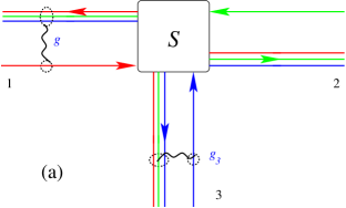
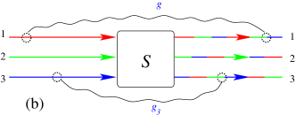
Figure 1: (Color online) (a) The geometry of a $Y$-junction is shown together with currents of incoming and outgoing fermions, the type of fermions in the scattered states representation is indicated by its color. The short-range interaction between the fermions is shown by wavy lines. (b) The equivalent representation in the chiral fermion basis after the unfolding procedure; the initially local interaction becomes non-local.

In terms of the triplet of incoming fermions $\Psi=(\psi_{1,in},\psi_{2,in},\psi_{3,in})$ the outgoing fermion operators may be expressed as $\Psi(x)=S\cdot\Psi(-x)\,$. Here the 3$\times$3 $S$-matrix characterizes the scattering at the junction and (up to irrelevant phase factors) has the structure

$$S =\begin{pmatrix}r_{1},&t_{12},&t_{13}\\ t_{21},&r_{1},&t_{23}\\ t_{31}&t_{32}&r_{2}\end{pmatrix}\,,$$ (2)

$$r_{1} =\tfrac{1}{2}\left(\cos\theta+e^{i\psi}\right)\sin\xi,\quad r_{2}=\cos\theta\,,$$

$$t_{13} =t_{32}=i\cos\tfrac{\xi}{2}\sin\theta,\quad t_{23}=t_{31}=i\sin\theta\sin\tfrac{\xi}{2}\,,$$

$$t_{12} =\cos\theta\cos^{2}\tfrac{\xi}{2}-e^{i\psi}\sin^{2}\tfrac{\xi}{2},\quad t_{21}=t_{12}|_{\xi\to\pi-\xi}\,.$$

We express the interaction term of the Hamiltonian in terms of density operators $\widehat{\rho}_{j,in}=\psi_{j,in}^{\dagger}\psi_{j,in}=\Psi^{+}\rho_{j}\Psi=\widehat{\rho}_{j}$, and $\widehat{\rho}_{j,out}=\psi_{j,out}^{\dagger}\psi_{j,out}=\Psi^{+}\widetilde{\rho}_{j}\Psi=\widehat{\widetilde{\rho}}_{j}$, where $\widetilde{\rho}_{j}=S^{+}\cdot\rho_{j}\cdot S$, as

$$H_{j}^{int}=2\pi\{g[\widehat{\rho}_{1}\widehat{\widetilde{\rho}}_{1}+\widehat{\rho}_{2}\widehat{\widetilde{\rho}}_{2}]+g_{3}\widehat{\rho}_{3}\widehat{\widetilde{\rho}}_{3}\}\Theta(x;-L,-l)\,.$$ (3)

The density matrices are given by $(\rho_{j})_{\alpha\beta}=\delta_{\alpha\beta}\delta_{\alpha j}$ and $(\widetilde{\rho}_{j})_{\alpha\beta}=S_{\alpha j}^{+}S_{j\beta}$. A convenient representation of 3$\times$3-matrices is in terms of Gell-Mann matrices $\lambda_{j}$, $j=0,1,\ldots,8$, the generators of $SU(3)$ (seeAristov and Wölfle (2011)). Notice that the interaction operator only involves $\lambda_{3}$ and $\lambda_{8}$ (besides the unit operator $(\lambda_{0})_{\alpha\beta}=\sqrt{2/3}\,\delta_{\alpha\beta}$). We note $Tr(\lambda_{j})=0$, $Tr(\lambda_{j}\lambda_{k})=2\delta_{jk}$, $j=1,\ldots,8$, and $[\lambda_{3},\lambda_{8}]=0$. Introducing a compact notation we define a three-component vector $\mathbf{\lambda}=(\lambda_{3},\lambda_{8},\lambda_{0})$, in terms of which the densitries may be expressed as $\rho_{j}=\sqrt{1/2}\sum_{\mu}R_{j\mu}\mathbf{\lambda}_{\mu}$, where the $3\times 3$ matrix $\mathbf{R}$ is defined as

$$\mathbf{R}=\left(\begin{array}[]{ccc}\frac{1}{\sqrt{2}}&\frac{1}{\sqrt{6}}&\frac{1}{\sqrt{3}}\\ -\frac{1}{\sqrt{2}}&\frac{1}{\sqrt{6}}&\frac{1}{\sqrt{3}}\\ 0&-\sqrt{\frac{2}{3}}&\frac{1}{\sqrt{3}}\end{array}\right)$$ (4)

and has the properties $\mathbf{R}^{-1}=\mathbf{R}^{T}$, $det\,\mathbf{R}=1$. The outgoing amplitudes are expressed in the analogous form with $\lambda_{j}$ replaced by $\widetilde{\lambda}_{j}=S^{+}\cdot\lambda_{j}\cdot S$ . With the aid of the $\lambda_{j}$ the $S$-matrix may be parametrized by eight angular variables (seeAristov (2011)). For the case under consideration only three of these, $\theta,\psi,\xi$, are relevant: $S=e^{i\lambda_{2}\xi/2}e^{i\lambda_{3}(\pi-\psi)}e^{i\lambda_{5}\theta}e^{i\lambda_{2}(\pi-\xi)/2}$ ; this $S$-matrix is given explicitly by Eq. (2). As will be shown below, the S-matrix and therefore the angular variables $\theta,\psi,\xi$, will be renormalized by the interaction.

Parametrization of conductance matrix. In the linear response regime, we may define a matrix of conductances $C_{jk}$ relating the current $I_{j}$ in lead $j$ (flowing towards the junction) to the electrical potential $V_{k}$ in lead $k$ : $I_{j}=\sum_{k}C_{jk}V_{k}$. The conductance matrix $\mathbf{C}$ has only three independent elements, which may be represented in the form of a $2\times 2$ antisymmetric matrix $\mathbf{G}$ with elements $G_{11}=G_{aa}=\frac{1}{2}(1-a)$, $G_{22}=G_{bb}=\frac{2}{3}(1-b)$, $G_{12}=-G_{21}=G_{ab}=\frac{c}{\sqrt{3}}$. These conductances relate the currents $I_{a}=\frac{1}{2}(I_{1}-I_{2})$, $I_{b}=\frac{1}{3}(I_{1}+I_{2}-2I_{3})$ to the bias voltages $V_{a}=(V_{1}-V_{2})$, $V_{b}=\frac{1}{2}(V_{1}+V_{2}-2V_{3})$.  It is useful to note that the nonzero elements of the matrix $\mathbf{C}^{R}=\mathbf{R}^{T}\cdot\mathbf{C\cdot R}$ are essentially the reduced conductances: $C_{11}^{R}=2G_{aa}$ , $C_{22}^{R}=(3/2)G_{bb}$ and $C_{12}^{R}=-C_{21}^{R}=\sqrt{3}G_{ab}$ , where the numerical factors arise due to the physically motivated asymmetric definitions of the currents and voltages. We now show that the parametrization of conductance in terms of $a$, $b$, $c$ follows quite naturally, by observing that the initial conductances are given by $C_{jk}=\delta_{jk}-Tr(\widetilde{\rho}_{j}^{r}\rho_{k})=\delta_{jk}-|S_{jk}^{r}|^{2}$, where the label $r$ indicates that the quantity is fully renormalized by interactions. Aristov and Wölfle (2011) By expressing $Y_{jk}=Tr(\widetilde{\rho}_{j}^{r}\rho_{k})$ in terms of $Y_{\mu\nu}^{R}=\frac{1}{2}Tr(\widetilde{\lambda}_{\mu}^{r}\lambda_{\nu})$ as $\mathbf{Y}=(\mathbf{R\cdot Y}^{R}\cdot\mathbf{R}^{T}\mathbf{)}$, we find by comparison with conductance matrix $\mathbf{C}^{R}$ that $\mathbf{Y}^{R}$ has nonzero elements given by the conductance parameters introduced above $Y_{11}^{R}=a$, $Y_{22}^{R}=b$, $Y_{12}^{R}=-Y_{21}^{R}=c$, $Y_{33}^{R}=1$. Therefore, we may use $\mathbf{Y}^{R}$ to represent the conductances in the renormalization group analysis below. By substituting the $S$-matrix in the form (2) into the definition of $\mathbf{Y}^{R}$, we find the relation of the $a$, $b$, $c$ to the angle variables: $a=-\frac{1}{2}(\cos^{2}\theta+1)\cos^{2}\xi+\cos\theta\cos\psi\sin^{2}\xi$, $b=\frac{1}{2}(3\cos^{2}\theta-1)$, $c=-\frac{\sqrt{3}}{2}\sin^{2}\theta\cos\xi$. We find therefore that $a,b,c$ are confined within the region $a\in[-1,1]$, $b\in[-1/2,1]$, $c\in[-\sqrt{3}/2,\sqrt{3}/2]$. The physically allowed points in $a$-$b$-$c$-space are inside a complex-shaped body labelled $B$ as shown in Fig. 2.

Figure 2: (Color online) Allowed values of conductances, $a,b,c$, lie inside the depicted body. The location of RG fixed points $N$, $A$, $\chi^{\pm}$, $M$ is also shown. The line of fixed points connecting FPs $A$ and $\chi^{+}$ is indicated in yellow.

Renormalization group equations. The renormalization of the conductances by the interaction is determined by first calculating the correction terms in each order of perturbation theory. We are in particular interested in the scale-dependent contributions proportional to $\Lambda=\ln(L/l)$ , where $L$ and $l$ are two above lengths, characterizing the interaction region in the wires. Here we only consider terms up to second order in $g,g_{3}$.

The conductances are given by $C_{jk}=\int_{-\infty}^{-L}dy\,\langle(\widehat{\rho}_{j}(-L)-\widehat{\widetilde{\rho}}_{j}(L))\widehat{\rho}_{k}(y)\rangle_{\omega\rightarrow 0}$. Here the combination $\widehat{\rho}_{j}(-L)-\widehat{\widetilde{\rho}}_{j}(L)$ means that the current is measured at $x=-L$, and integration over $y$ for the incoming densities corresponds to the notion of voltage, $V_{k}$, applied to the leads; in the considered limit $\omega L\rightarrow 0$ the value of $L$ in this definition does not play a role. Aristov and Wölfle (2009) The quantum averaging $\langle\ldots\rangle$ is accompanied by taking trace over the matrices’ product. Up to second order we need to consider the contributions depicted in Fig. 4 of Ref. Aristov et al. (2010). Differentiating these results with respect to $\Lambda$ (and then putting $\Lambda=0$) we find the RG equations up to second order in the interaction

$$\tfrac{d}{d\Lambda}Y_{\mu\nu}^{R}=-\tfrac{1}{2}Tr\left(\widehat{W}^{R}_{\mu\nu}\widehat{W}^{R}_{\mu^{\prime}\nu^{\prime}}\right)(g_{\nu^{\prime}\mu^{\prime}}^{R}+\tfrac{1}{2}g_{\nu^{\prime}\kappa}^{R}Y_{\kappa\kappa^{\prime}}^{R}g_{\kappa^{\prime}\mu^{\prime}}^{R})\,.$$

Here the $\widehat{W}^{R}_{\mu\nu}=(\mathbf{R}^{T}\cdot\widehat{\mathbf{W}}\cdot\mathbf{R)}_{\mu\nu}=\frac{1}{2}[\lambda_{\mu},\widetilde{\lambda}_{\nu}]$, and $\widehat{W}_{jk}=[\rho_{j},\widetilde{\rho}_{k}]$, are 3$\times$3 matrices for each pair of $\mu\nu$ (or $jk$) and the trace operation $Tr$ is defined with respect to that matrix space, whereas $g_{\mu\nu}^{R}=(\mathbf{R}^{T}\cdot\mathbf{g\cdot R)}_{\mu\nu}$, with $g_{jk}=\delta_{jk}g_{j}$ and $Y_{\kappa\kappa^{\prime}}^{R}$ are scalars with respect to this space (sums over repeated indices are implied). The nine matrices $\widehat{W}^{R}_{\mu\nu}$ may be evaluated best with the aid of computer algebra, inserting the $S$-matrix in terms of the quantities $a,b,c$, as given above. As a result one finds the following set of RG-equations

$$\tfrac{da}{d\Lambda} = \beta_{a}=\tfrac{g}{2}(A_{1}+\tfrac{1}{\kappa}A_{2}+\tfrac{g}{4}A_{3})\,,$$

$$\tfrac{db}{d\Lambda} = \beta_{b}=\tfrac{g}{2}(A_{2}+\tfrac{1}{\kappa}B_{2}+\tfrac{g}{4}B_{3})\,,$$ (5)

$$\tfrac{dc}{d\Lambda} = \beta_{c}=-c\tfrac{g}{2}[1+2a+\tfrac{1}{\kappa}(1+2b)+\tfrac{g}{4}C_{3}]\,,$$

where we defined

$$A_{1} =1+b-2a^{2},\quad A_{2}=a(1-b)+c^{2}\,,$$ (6)

$$B_{2} =(1-b)(1+2b),$$

$$A_{3} =a(3+b-4a^{2})+c^{2}+\tfrac{2}{\kappa}(ab-a+c^{2}(4a+1))$$

$$+\tfrac{1}{\kappa^{2}}(1+2b)(a-ab+c^{2})\,,$$

$$B_{3} =(1-b)\left(2a^{2}+2b+1\right)+2ac^{2}$$

$$+\tfrac{2}{\kappa}(2b+1)\left(b+2c^{2}-1\right)+\tfrac{1}{\kappa^{2}}(1+3b-4b^{3})\,,$$

$$C_{3} =4a^{2}+2a+2b+1-\tfrac{2}{\kappa}\left(a(1-b)+3\left(b+c^{2}\right)\right)$$

$$+\tfrac{1}{\kappa^{2}}(2b+1)^{2}\,,$$

and $\kappa=3g/(g+2g_{3})$.

Fixed points of RG flow. The fixed points of the above RG equations may be found analytically. For general (but small) values of $g,g_{3}$ we find five fixed points in total, labelled $N,A,M,\chi^{+},\chi^{-}$. At fixed point $N$ we have $a=b=1$ and $c=0$. It corresponds to the complete separation of all wires and $G_{aa}=G_{bb}=G_{ab}=0$. The approach to the fixed point is given by the power laws $G_{bb}\propto L^{-\gamma_{1}^{N}}$  and $4G_{aa}-G_{bb}\propto L^{-\gamma_{2}^{N}}$ with exponents $\gamma_{1}^{N}=g+g_{3}+g^{2}/2$ and $\gamma_{2}^{N}=2g+g^{2}$. The third direction of RG flow, along the $c$ axis in Fig. 2, is unaccessible due to unitarity restrictions, see Aristov (2011). This fixed point is the only stable one for repulsive interaction, either $g>0$ or $g_{3}>0$, or both.

Fixed point $A$ is characterized by $a=-1$, $b=1$, $c=0$ corresponding to $G_{aa}=1$, $G_{bb}=G_{ab}=0$ and thus the situation of a perfect wire 1-2, detached from wire $3$. Stability analysis shows that it is stable for attractive interaction, $g<0$, provided $g_{3}+g^{2}/2>0$. The critical exponents at $A$ are defined as $4(G_{aa}-1)+G_{bb}\propto L^{-\gamma_{1}^{A}}$ and $G_{bb},G_{cc}\propto L^{-\gamma_{2}^{A}}$ and are given by $\gamma_{1}^{A}=2g-g^{2}$, $\gamma_{2}^{A}=-g_{3}-g^{2}/2$.

Fixed point $M$ is characterized by noninteger values of the conductance, which are found to depend on the strength of interaction, $a\simeq-\kappa/3+gh$, $b\simeq(\kappa^{2}/3-1)/2-g\kappa h$, $c=0$, with $h=\kappa(\kappa-1)/6$. It is stable for $g>0$ and $g_{3}<0$ in a region depicted in Fig. 3. The critical exponents at $M$ are obtained as $\gamma_{1}^{M}\simeq g(\kappa-9\kappa^{-1})/12$, $\gamma_{2}^{M}\simeq-g(\kappa+3\kappa^{-1})/2$ and $\gamma_{3}^{M}\simeq g(3-\kappa)/6$, in the scaling laws $\frac{4\kappa}{3}G_{aa}+G_{bb}-\big{(}1+\frac{\kappa}{3}\big{)}^{2}\propto L^{-\gamma_{1}^{M}}$, $\frac{\kappa^{2}-9}{6\kappa}G_{aa}+G_{bb}+\frac{(\kappa-3)^{2}(\kappa+3)}{12\kappa}\propto L^{-\gamma_{2}^{M}}$, and $G_{cc}\propto L^{-\gamma_{3}^{M}}$. The region of stability of $M$ corresponds to $0<g\lesssim-g_{3}$, which translates to $-3\lesssim\kappa<0$, in which range all $\gamma_{i}^{M}>0$.

Whereas fixed points $N,A,M$ exist also in the absence of magnetic flux, two new (stable) fixed points, $\chi^{\pm}$, appear as a result of the broken time reversal symmetry. These are the fixed points of maximum chirality first discussed in Chamon et al. (2003); Oshikawa et al. (2006). The corresponding fixed point values are $a=b=-\frac{1}{2}$ and $c=\pm\frac{1}{2}\sqrt{3}$ , or in terms of conductances: $G_{aa}=\frac{3}{4}$ , $G_{bb}=\frac{1}{2}$, and $G_{ab}=-G_{ba}=\pm\frac{1}{2}$. The fixed points $\chi^{\pm}$ are stable for attractive interaction, $g,g_{3}<0$, in the domain $|g_{3}|>g^{2}$ (see Fig.3). In this case the conductances are not quantized in integer units of the conductance but assume fractional values. The two fixed points $\chi^{\pm}$ are located symmetrically to the plane $c=0$ in $a$-$b$-$c$-space. Depending on whether the initial condition for $c$ is $c_{in}>0$ or $c_{in}<0$ the RG-flow will tend to $\chi^{+}$ or $\chi^{-}$. If $c_{in}=0$ the flow will stay in the $c=0$ plane; the $M$ point is stable in place of $\chi^{\pm}$ in this caseAristov and Wölfle (2011). The critical exponents at $\chi^{\pm}$ are found as $\gamma_{1}^{\chi}=g$ and $\gamma_{2}^{\chi}=g_{3}+g^{2}/2$.

In the case $g_{3}=g$ the values of the critical exponents at the fixed points $N$, $A$, $\chi^{\pm}$ obtained here agree with the results quoted in the literature Chamon et al. (2003); Oshikawa et al. (2006). The comparison of our results with those obtained by the bosonization method is nontrivial, since the latter are valid for infinite TLL wires, whereas our method provides results for the experimentally relevant case of finite TLL wires attached to ideal leads. Following earlier works, Oshikawa et al. Oshikawa et al. (2006) have defined a prescription for calculating the conductances ${C}_{ij}$ of wires attached to ideal leads from the conductances ${\bar{C}}_{ij}$ of the infinite wire system, see Sec. 12 therein. In the following we shall use their recipe for converting ${\bar{C}}_{ij}$ into ${C}_{ij}$.

Fixed point $M$ requires special consideration. Its existence had been first conjectured inChamon et al. (2003); Oshikawa et al. (2006), but its properties were not accessible. Later fixed point $M$ was clearly identified in numerical studies using the functional renormalization group method Barnabé-Thériault et al. (2005). The above values of the critical exponents [see also Aristov and Wölfle (2011)], $\gamma_{2}^{M}=-2g\simeq 2(K-1)$ and $\gamma_{3}^{M}=g/3\simeq(1-K)/3$, with $K=\sqrt{(1-g)/(1+g)}$ the Luttinger parameter, are in agreement with the numerical estimates obtained in Barnabé-Thériault et al. (2005). Recent numerical results Rahmani et al. (2010) on the values of conductances ${\bar{C}}_{ij}$ at $\chi^{\pm}$ and $M$ obtained via the Density Matrix Renormalization Group (DMRG) method confirm the known analytical results for the $\chi^{\pm}$ fixed points, in agreement with our results. In Ref. Aristov and Wölfle (2011) (see also above) we found the value of the conductances at the $M$ point, $C_{ij}=\frac{4}{9}(3\delta_{ij}-1)$, independent of the strength of interaction, $g=g_{3}$. Expressing the results in terms of conductances ${\bar{C}}_{ij}$, we find ${\bar{C}}_{ij}=C_{ij}\frac{3K}{2+K}$. The component ${\bar{C}}_{12}$ agrees very well with the numerical estimate given in Rahmani et al. (2010), lending support to our identification of the fixed point $M$ with the “mysterious” fixed point in Oshikawa et al. (2006).

It is worth noting that in the region of stability of the $M$ point the initial Hall conductance scales to zero, meaning that the magnetic flux will be screened (this is also true when the $N$ or $A$ points are stable, but for a trivial reason, since at least one of the wires gets separated in that case). In Fig. 2 we show the location of the fixed points in $a$-$b$-$c$-space for a typical choice of interaction constants. All fixed points are located at the surface of the body $B$.

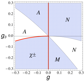
Figure 3: (Color online) The RG phase portrait, showing regions of stability of fixed points in the space of interactions $g$ and $g_{3}$. The M point only exists in the shaded regions. Lines of fixed points appear for $g,g_{3}$ values located along the red (thick) lines.

Lines of fixed points. As discussed above, the line $g_{3}+g^{2}/2=0$ in the space of interaction constants separates two domains in which fixed point $\chi^{+}$ (or $\chi^{-}$) or $A$ are stable. For $g$, $g_{3}$ on that line, in addition to the two fixed points $A,\chi^{\pm}$ we find a whole line of stable fixed points connecting these two. This means that the RG flow may stop at any point on this line, depending on the initial conditions. The fixed point line is parametrized by $a=-1+\frac{1}{2}\tau$, $b=1-\frac{3}{2}\tau$, $c=\frac{\sqrt{3}}{2}\tau$, with $\tau\in[0,1]$. Substituting this parametrization into the above RG-equations, we find $\frac{d}{d\Lambda}\{a,b,c\}=-\frac{1}{2}(g_{3}+g^{2}/2)\tau(1-\tau)\{1,-3,\sqrt{3}\}$, demonstrating that on the line $A$–$\chi^{\pm}$ and for $(g_{3}+g^{2}/2)\neq 0$ the flow is directed along the line, towards $A$ or $\chi^{\pm}$, depending on whether $-g_{3}<g^{2}/2$ or the opposite. When $g_{3}=-g^{2}/2$ the RG flow is directed perpendicular to this line with the exponents $g(1\pm\sqrt{1-\tau})$, i.e. the fixed points on the line are stable. This is demonstrated in Fig. 4 where the RG-trajectories on the surface of body $B$ are shown for different $g,g_{3}$ and different initial conditions. We observe that the blue and green trajectories for interaction strengths in the regions of interaction parameter space labeled $\chi^{+}$ and $A$ terminate at the respective fixed points (note that the line at $\theta=\pi$ corresponds to a single point), whereas the red lines calculated for interaction values at the boundary between those two regions are found to terminate at any point along the lines connecting $A$ and $\chi^{+}$.

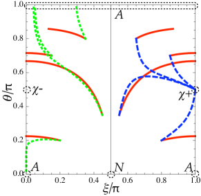
Figure 4: (Color online) RG trajectories on the surface $\psi=0$ red (solid): $g=-0.333$, $g_{3}=-0.062$, blue (dashed): $g=-0.25$, $g_{3}=-0.25$, green (dotted): $g=-0.4$, $g_{3}=-0.01$.

There is a second line of fixed points, separating the domain of stability of the fixed points $M$ ($g>0,g_{3}<0$) and $\chi^{+,-}$ ($g<0,g_{3}<0$). It is realized for any $g_{3}<0$ at $g=0$. The line of fixed points connects fixed points $M$ and $\chi^{\pm}$ and is parametrized by $a=-\frac{1}{2}\tau^{2}$, $b=-\frac{1}{2}$, $c=\frac{\sqrt{3}}{2}\tau$, with $\tau\in[-1,1]$. Finally, a trivial line of fixed points exists for any $g_{3}>0$ at $g=0$. It connects the fixed points $A$ and $N$ and corresponds to the interacting third wire, being detached from the non-interacting wire 1–2 of arbitrary conductance, $a\in[-1,1]$, $b=1$, $c=0$. Evidently, $a$ should not be renormalized in this case.

The present weak coupling theory may be extended into the strong coupling regime, using the approach in Aristov and Wölfle (2011), confirming the existence of lines of fixed points.

Conclusion. In this paper we developed a fermionic description of a Y-junction (1–2 symmetric junction of three TLL-wires) threaded by magnetic flux, in the regime of weak interaction. In this case the conductance matrix has three independent components, the conductance associated (i) with current flowing in wires $1$ and $2$, (ii) with current flowing from wire $3$ into wires $1,2$, (iii) with current in wires $1,2$, driven by a voltage drop in wire $3$ (Hall conductance). We calculated the scale dependent contributions to the conductances up to order $g^{2}$ and $g_{3}$ in the interaction constants. From there we derived three renormalization group equations for the conductances. These equations have five fixed points labelled $N,A,M,\chi^{+},\chi^{-}$. When both interactions are repulsive ($g>0$ and $g_{3}>0$) only $N$ is stable, which corresponds to the total separation of the wires. If at least one interaction is attractive ($g$ and/or $g_{3}<0$), we find four regions in $g_{3}$–$g$-space in which $N,A,\chi^{\pm},M$ are stable, respectively. At the two border-lines separating regions of stability of $A,\chi^{\pm}$ (the line $g_{3}+g^{2}/2=0$) and of $\chi^{\pm},M$ (the line $g=0$, $g_{3}<0$), respectively, we find a novel and unexpected situation: at these lines in $g_{3}$–$g$-space not only the two stable fixed points assigned to the adjacent regions are stable, but a whole line of fixed points connecting those two fixed points becomes stable. We have checked that the leading higher order terms do not destroy the fixed line property (to be published). We conjecture that this is an incidence of a more general phenomenon: whenever two regions in interaction constant space with different stable fixed points touch, and the two fixed points neither vanish nor merge at the contact manifold, a whole line of stable fixed points connecting the two initial fixed points emerges.

We thank A. Nersesyan, J. Schmalian, V.Yu. Kachorovskii, A.P. Dmitriev and especially I.V. Gornyi and D.G. Polyakov for useful discussions. The work of D.A. was supported by the German-Israeli Foundation (GIF), the Dynasty foundation, and a RFBR grant. The work of D.A. and P.W. was supported by the DFG-Center for Functional Nanostructures at KIT.

References

- Giamarchi (2003) T. Giamarchi, Quantum Physics in One Dimension (Clarendon Press, Oxford, 2003).
- Kane and Fisher (1992) C. L. Kane and M. P. A. Fisher, Phys. Rev. B 46, 15233 (1992).
- Furusaki and Nagaosa (1993) A. Furusaki and N. Nagaosa, Phys. Rev. B 47, 4631 (1993).
- Weiss et al. (1995) U. Weiss, R. Egger, and M. Sassetti, Phys. Rev. B 52, 16707 (1995).
- Fendley et al. (1995) P. Fendley, A. W. W. Ludwig, and H. Saleur, Phys. Rev. B 52, 8934 (1995).
- Yue et al. (1994) D. Yue, L. I. Glazman, and K. A. Matveev, Phys. Rev. B 49, 1966 (1994).
- Polyakov and Gornyi (2003) D. G. Polyakov and I. V. Gornyi, Phys. Rev. B 68, 035421 (2003).
- Das et al. (2004) S. Das, S. Rao, and D. Sen, Phys. Rev. B 70, 085318 (2004).
- Lal et al. (2002) S. Lal, S. Rao, and D. Sen, Phys. Rev. B 66, 165327 (2002).
- Aristov and Wölfle (2009) D. N. Aristov and P. Wölfle, Phys. Rev. B 80, 045109 (2009).
- Chamon et al. (2003) C. Chamon, M. Oshikawa, and I. Affleck, Phys. Rev. Lett. 91, 206403 (2003).
- Oshikawa et al. (2006) M. Oshikawa, C. Chamon, and I. Affleck, J. Stat. Mech. 2006, P02008 (2006).
- Barnabé-Thériault et al. (2005) X. Barnabé-Thériault, A. Sedeki, V. Meden, and K. Schönhammer, Phys. Rev. Lett. 94, 136405 (2005).
- Bellazzini et al. (2007) B. Bellazzini, M. Mintchev, and P. Sorba, Journal of Physics A: Mathematical and Theoretical 40, 2485 (2007).
- Hou and Chamon (2008) C.-Y. Hou and C. Chamon, Phys. Rev. B 77, 155422 (2008).
- Hou et al. (2009) C.-Y. Hou, E.-A. Kim, and C. Chamon, Phys. Rev. Lett. 102, 076602 (2009).
- Das and Rao (2011) S. Das and S. Rao, Phys. Rev. Lett. 106, 236403 (2011).
- Steinberg et al. (2008) H. Steinberg, G. Barak, A. Yacoby, L. N. Pfeiffer, K. W. West, B. I. Halperin, and K. Le Hur, Nature Physics 4, 116 (2008).
- Meden et al. (2008) V. Meden, S. Andergassen, T. Enss, H. Schoeller, and K. Schönhammer, New Journal of Physics 10, 045012 (2008).
- Aristov et al. (2010) D. N. Aristov, A. P. Dmitriev, I. V. Gornyi, V. Y. Kachorovskii, D. G. Polyakov, and P. Wölfle, Phys. Rev. Lett. 105, 266404 (2010).
- Aristov and Wölfle (2011) D. N. Aristov and P. Wölfle, Phys. Rev. B 84, 155426 (2011).
- (22) “Lines of fixed points” discussed in Barnabé-Thériault et al. (2005) correspond to one point () in terms of conductance.
- Aristov (2011) D. N. Aristov, Phys. Rev. B 83, 115446 (2011).
- Rahmani et al. (2010) A. Rahmani, C.-Y. Hou, A. Feiguin, C. Chamon, and I. Affleck, Phys. Rev. Lett. 105, 226803 (2010).