LMU-ASC 46/11
A new determination of from hadronic decays
Diogo Boito,a Oscar Catà,b,c Maarten Golterman,d Matthias Jamin,e Kim Maltman,f,g James Osborne,d Santiago Perisd111Permanent address: Departament de Física, Universitat Autonòma de Barcelona, E-08193 Bellaterra, Barcelona, Spain
aDepartament de Física and IFAE
Universitat Autonòma de Barcelona, E-08193 Bellaterra, Barcelona, Spain
bDepartament de Física Teòrica and IFIC
Universitat de València-CSIC, E-46071 València, Spain
cLudwig-Maximilians-Universität München, Fakultät für Physik
Arnold Sommerfeld Center for Theoretical Physics, D–80333 München, Germany
dDepartment of Physics and Astronomy
San Francisco State University, San Francisco, CA 94132, USA
eInstitució Catalana de Recerca i Estudis Avançats (ICREA)
IFAE, Universitat Autonòma de Barcelona
E-08193 Bellaterra,
Barcelona, Spain
fDepartment of Mathematics and Statistics
York University, Toronto, ON Canada M3J 1P3
gCSSM, University of Adelaide, Adelaide, SA 5005 Australia
ABSTRACT
We present a new framework for the extraction of the strong coupling from hadronic decays through finite-energy sum rules. Our focus is on the small, but still significant non-perturbative effects that, in principle, affect both the central value and the systematic error. We employ a quantitative model in order to accommodate violations of quark-hadron duality, and enforce a consistent treatment of the higher-dimensional contributions of the Operator Product Expansion to our sum rules. Using 1998 OPAL data for the non-strange isovector vector and axial-vector spectral functions, we find the values in fixed-order perturbation theory, and in contour-improved perturbation theory. For comparison, the original OPAL analysis of the same data led to the values (fixed-order) and (contour-improved).
I Introduction
In the past few years there has been a renewed interest in the precision determination of from non-strange hadronic decays. One reason for this interest is the recent calculation of the coefficient of the term in the perturbative contribution to the Adler function PT . This contribution dominates the ratio of the hadronic decay width and the electronic decay rate BNP ,
| (1) |
Another reason is the existence of a number of competing analysis methods which lead to results that are not, or only barely, consistent with one another. In fact, the error on from decays quoted in a recent (2009) review SB09 has gone since its 2006 version, for the simple reason that the result of Ref. SB09 was obtained by averaging the central values of all recent decay determinations of and the error by considering the spread of these central values. All determinations are based on data from (primarily) the ALEPH (see Ref. ALEPH98 for their 1998 analysis and Ref. ALEPH for their 2005 analysis) and (also) the OPAL (see Ref. OPAL ) collaborations; the differences in the results are on the theory side.
Clearly, this is an unsatisfactory situation. There are at least three theoretical issues related to the discrepancies between the different determinations. Number one is the long-standing question as to which resummation scheme, fixed-order perturbation theory (FOPT) or contour-improved perturbation theory (CIPT), is best used for evaluating the perturbative contributions to . Many of the recent reanalyses have focussed on this question PT ; Davieretal08 ; BJ ; Menke ; CF ; DM . Much less attention has been devoted to the two other issues, both of which concern non-perturbative contributions to . Because of the relatively low value of the mass, such contributions cannot be entirely neglected, even if they are expected to be small. Issue number two is the question of whether the Operator Product Expansion (OPE) contributions beyond perturbation theory have been consistently taken into account. Here we are aware of only one systematic investigation MY , in which it was demonstrated that self-consistency problems existed for a number of earlier analyses. Specifically, it was shown that the OPE parameters obtained in those analyses do not provide a good match between data and theory when the upper limit on the hadronic invariant mass-squared, , in the weighted integrals over the spectral functions (which enter the finite-energy sum rules (FESRs) employed in these analyses) is varied away from .111Some of the earlier analyses carried out this test for the FESR based on the kinematic weight (the weight yielding when ), for which it works reasonably well. Reference MY showed that these analyses unambiguously fail the tests for other doubly-pinched FESRs. Issue number three concerns potential violations of “quark-hadron duality” not taken into account in previous FESR determinations of . In the case of FESRs, the assumption of quark-hadron duality amounts to presuming that all non-perturbative effects are accounted for by higher-dimensional terms in the OPE. To date, this assumption has not seen a systematic investigation. As already explained in Ref. MY , the issues of the OPE and possible violations of quark-hadron duality are intricately connected: without a quantitative analysis of duality violations, it turns out to be difficult to treat the OPE consistently without relying on “external” results. For instance, in the analysis of Ref. MY , the dimension-4 term in the OPE had to be fixed using a result for the gluon condensate from charmonium sum rules.
In this article, we aim to address this situation, focussing on the non-perturbative questions. We use a recently developed model for the duality-violating (DV) part of the -flavor vector () and axial-vector () spectral functions CGP , which makes it possible to carry out a self-contained FESR analysis in which stability with respect to varying is checked self-consistently without reliance on external values for any of the OPE parameters.
Since no QCD-based theory of quark-hadron duality exists, we have to resort to a model. This means that our results will be based on the (testable) assumption that this model gives a good description of the DV part of the spectral functions for values of from down to a minimum value, , sufficiently low to lie in the range kinematically accessible in hadronic decays. We emphasize that the need to make such an assumption has always been a fundamental “shortcoming” of the determination of from decays. Assuming quark-hadron duality a priori, and therefore neglecting the effect of DVs altogether, also amounts to employing a – probably worse – model. In other words, in order to investigate the systematics related to the assumption of quark-hadron duality, one cannot avoid the adoption of a model of the DV part of the spectral functions. In Ref. CGP it was found that the model we intend to employ gives a reasonable description of the spectral functions in the region .222In the present, more detailed analysis, we will find that a significantly larger value of is preferred. Moreover, the physics of our model is based on a picture of the hadron resonances which are experimentally seen in the spectral function. Resonances are not described by perturbation theory or the OPE, and thus should be part of any model aiming to describe violations of quark-hadron duality.
In this work, we do not address the issue of the optimal choice of resummation for the truncated perturbative series in a given FESR. While this systematic, of course, forms a potentially important part of the final theory error on , we have no new elements to add to the discussion of this issue. Moreover, we believe that the non-perturbative part of the systematics should be understood first, in order to get a more reliable picture of the quantitative discrepancy between results based on FOPT and CIPT. We will therefore carry out our whole analysis with both resummation schemes.
To date, two experiments, ALEPH ALEPH98 ; ALEPH and OPAL OPAL , have made the non-strange and spectral functions from their -decay analyses publicly available. The 2005 analysis of ALEPH is more recent, and based on more statistics, and thus would be expected to have smaller experimental errors. Unfortunately, the 2005 ALEPH data cannot be used at present, because correlations due to unfolding have been inadvertently omitted in the original ALEPH analysis and hence from the publicly posted covariance matrices TAU2010 .333We thank members of the ALEPH collaboration for private communications, in which the existence of this problem has been confirmed. Since the re-analysis of the ALEPH data has yet to be completed, we limit ourselves, in this article, to an analysis employing the OPAL data.
In order to normalize the various exclusive-mode components of the spectral functions, OPAL relied on the branching fractions available in 1998, as well as the then-current values of and the electronic branching fraction . All of these have been updated since then, and this makes it possible to at least partially update the OPAL inclusive spectral distributions as well. Such an update would allow an updated, though still OPAL-based, determination of . Here, since our primary goal is to investigate the impact of the novel features of our treatment of non-perturbative effects on the extracted results for , we choose not to perform this update, and instead work with the data in precisely the same form as used by OPAL OPAL . We plan to devote a separate article to an adaptation of OPAL data to recent values of the exclusive branching fractions, and , and an investigation of the effect of this adaptation on the value of and other OPE parameters.
This article is organized as follows. In Sec. II we present a brief review of the application of FESRs to hadronic decays, with emphasis on the issue of quark-hadron duality. In Sec. III we are then able to provide a more thorough discussion of the various systematic errors discussed already above. Preparing for a presentation of our results in Sec. VI, we describe the theory parametrization we will employ in more detail in Sec. IV, and discuss the issue of strong correlations in the integrated data, and our resulting fitting strategies, in Sec. V. Apart from reporting on our fits in Secs. VI.1 and VI.2, we consider also, in Sec. VI.4, the channel sum (related to the non-strange part of ) as well as the channel difference. In the latter case, we demonstrate that our fit results satisfy the Weinberg sum rules SW as well as the DGMLY sum rule for the electromagnetic mass difference EMpion . Section VII contains a summary of our results, including a conversion of to its value at the mass; Sec. VIII contains our conclusions.
II Theory summary
Our analysis will involve the correlation functions
where is one of the non-strange or currents, or , and the superscripts and label the spin. The decomposition in the third line employs the combinations and , which are free of kinematic singularities. Defining and the spectral functions
| (3) |
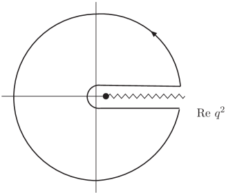
Cauchy’s theorem and the analytical properties of , applied to the contour in Fig. 1, imply the FESR relation
| (4) |
valid for any and any weight analytic in the region of the contour shankar . In the present work we will restrict ourselves to polynomial weights. Partial integration allows the right-hand side of Eq. (4) to be recast in terms of the Adler function
| (5) |
The spectral functions are measurable in hadronic decays. Explicitly, for Standard Model decays induced by the flavor (isovector) currents, with , , and the scaled, non-strange and widths
| (6) |
one has tsai
| (7) |
in which is defined by
| (8) |
where is a short-distance electroweak correction. Since, in the Standard Model,
| (9) | |||||
the differential distributions proportional to the expression in square brackets in Eq. (8) provide a direct measure of , up to numerically negligible corrections.444The decay constant, MeV PDG , is presently known very accurately. The central value of the branching fraction, , employed in the 1998 OPAL analysis corresponds to the somewhat larger value MeV. In order to match exactly the OPAL treatment of the and spectral functions we employ the latter value in our analysis. Note that, since was obtained by the PDG in a combined fit to the full set of basis modes, it would, in fact, be inconsistent to change just without simultaneously changing all other branching fractions. We will revert to the updated value MeV in our later analysis employing updated OPAL data. The second delta function in Eq. (9), which comes from the kinematic singularity present in , does not contribute to the integral in Eq. (8) as a result of the factor of in the accompanying weight .
For sufficiently large , and ignoring for a moment that the OPE is only valid for large euclidean , the right-hand side of Eq. (4) can be approximated using the OPE for . Experimental spectral data can then be used to fit the OPE, and extract parameters such as BNP . In what follows, we will denote the experimental version of the spectral integral on the left-hand side of Eq. (4) by (generically, ) and the theoretical representation of the contour integral on the right-hand side by (generically, ).
In the upper part of the energy region allowed by -decay kinematics is dominated by its dimension contribution, i.e., the perturbative contribution in the chiral limit.555Perturbative contributions proportional to powers of the quark masses are included in OPE terms. The perturbative expression for the Adler-function (5), which is known to order PT , can be written as666See, for instance, Ref. MJ .
| (10) |
with . Since is independent of , we can choose , indicating that only the coefficients are independent; all other can be expressed in terms of the through the renormalization group. In the scheme, , , and PT . We will use the guess of Ref. BJ for the next coefficient, assigning an uncertainty of in order to estimate the error due to truncating perturbation theory (cf. Sec. VI.3).
The freedom to choose in Eq. (10) is at the heart of the different prescriptions employed for evaluating the perturbative contribution to the right-hand side of Eq. (4): in FOPT, is used in Eq. (10), whereas in CIPT is employed inside the contour integral on the right-hand side of Eq. (4) CIPT .
Beyond perturbation theory, one may improve the approximation to the right-hand side of Eq. (4) by including higher-dimension contributions to . Explicitly,
| (11) |
with the OPE coefficients logarithmically dependent on through perturbative corrections. The term with corresponds to the purely perturbative, mass-independent contributions, represented by Eq. (10). The , with , contain non-perturbative condensate contributions, and are, in principle, different for the and channels.
We will neglect , which is purely perturbative and quadratic in the light quark masses.777Since in the present study we are only dealing with the light up- and down-quark correlators, the mass-squared corrections are tiny. Still, one version of our analysis code has implemented all known corrections up to , and we have verified that they are indeed negligible. It has been suggested that a non-perturbative term should be added in order to account for the truncation of the perturbative series for the term NZ . We postpone an investigation of this issue to future work, and here set .
Neglecting contributions of or proportional to , both of which are numerically very small, the coefficient is a linear combination of the “gluon condensate” (with the gluon field strength), and the chiral condensates , . To leading order in both contributions to are the same in the and channels. Differences in the and light quark condensate contributions enter beginning at or NLOC4 .
The coefficient is assumed to be dominated by four-quark condensates, because the contribution from vanishes at leading order in D6 , and the contributions from lower-dimensional operators are suppressed by powers of the quark mass. Coefficient functions for the four-quark condensates were calculated to next-to-leading order in Ref. D64quark . At there is a proliferation of operators, and very little detailed information is available. As we will explain in Sec. IV below, we will not need to consider terms with .
The OPE is valid when the euclidean distance in Eq. (II) is small compared to , or, equivalently, when euclidean is positive and large. However, both perturbation theory and the OPE are expected to break down near the positive real axis PQW . We may account for this additional non-perturbative effect by writing the right-hand side of Eq. (4) as CGP
| (12) |
with
| (13) |
The difference defines the duality violating contribution to .
All previous determinations of from hadronic decays have assumed, implicitly or explicitly, that integrated DV contributions are small enough to be neglected for the weights employed in the analysis. While this assumption has sometimes been checked for self-consistency (see, e.g., Ref. MY ), a comprehensive quantitative estimate of the impact of DVs on the precision with which can be determined has not been provided. One of the aims of the present work is to provide a comprehensive analysis which takes DVs into account, and hence remedies this shortcoming.
As shown in Ref. CGP , if is assumed to decay fast enough as , the right-hand side of the FESR relation (4) can be rewritten as
| (14) |
with
| (15) |
The imaginary parts can be interpreted as the DV parts, , of the spectral functions. Following Ref. CGP , we will parametrize as
| (16) |
This introduces, in addition to and the OPE condensates, four new parameters in each channel. The OPE, supplemented by the ansatz (16), will be assumed to hold for , where will have to be inferred from fits to the experimental data. The extended analysis, including DVs, will of course only be possible if lies significantly below .
The ansatz (16) is modeled on the asymptotic behavior for large of a semi-realistic model for the QCD spectrum in a given channel. This model was developed in Ref. CGPmodel , based on earlier ideas described in Ref. russians . It incorporates a combination of large- insights (narrow resonances with widths increasing with mass) as well as the Regge picture for the spacing between resonances. These ingredients lead quite naturally to the exponential decay in Eq. (16) with the decay parameter , as well as the oscillatory behavior represented by the sine function, both with arguments (approximately) linear in . We favor this model over other attempts to model DVs because of its natural connection to the resonance structure of the spectral distributions, something that is not evident in other models (such as those based on instantons). For detailed discussions of the model, see Refs. CGPmodel ; CGP05 ; MJ11 .
III Systematic errors
There are three sources of systematic error affecting, to various extents, existing FESR determinations of . Since the investigation of two of these sources is the central aim of this work, we briefly describe each of the three sources here, before embarking on the details of our analysis.
-
1.
There are (at least) two ways of partially resumming the perturbative contribution to , CIPT and FOPT (cf. Sec. II). The relative merits of the two methods have been the subject of a number of investigations PT ; Davieretal08 ; BJ ; Menke ; CF ; DM . While no particular preference is given to either scheme in Refs. PT ; DM , CIPT is favored in Davieretal08 ; Menke , whereas Refs. BJ ; CF give arguments in favor of FOPT, in the latter work through a new CI expansion in a conformally mapped coupling.
We will not attempt to resolve the associated systematic uncertainty in this work, but instead report on the results of our fits using both CIPT and FOPT. In fact, it is interesting to see what discrepancy remains between CIPT and FOPT after other systematic errors, described below, have been properly taken into account.
-
2.
With the exception of Ref. MY , the OPE has not been treated consistently in previous extractions of from decays, in the sense we now explain. Consider a term of order in the OPE of Eq. (11). The dominant term in the expansion in of the corresponding coefficient , , is a constant of order one (times the relevant condensate). In the sum rule (4), this term in the OPE is picked out by the term of degree in the weight . Other terms in will also pick up contributions from , because of the logarithmic dependence of on , but such contributions will not be dominant as they are suppressed by at least one extra power of . Thus, if weight functions up to degree are used in the fits, it follows that terms up to at least order must be kept in the OPE in order to retain all potentially relevant contributions not suppressed by at least one extra power of .
In the conventional analysis of Refs. ALEPH ; OPAL ; Davieretal08 ; DP1992 this was not done: while weights up to degree in were employed (which would generally require keeping terms in the OPE up to ()), only terms up to () were retained. As noted earlier, it was found in Ref. MY that this is not self-consistent: with the parameter values found in those fits, the dependence of the theory curves does not match that of the data for the majority of the weights employed, as well as for alternate degree 2 and 3 weights which explicitly test the parameters obtained from the original fits.888See also Ref. CGPmodel , where it was shown in a model study that adding a term to the OPE in an analysis like that of Refs. ALEPH ; Davieretal08 ; OPAL can make a significant difference. In this work, we will restrict ourselves to weight functions of degree , corresponding to keeping terms up to in the OPE. As we will explain below, this implies we will have to vary in the FESR (4); it is not possible to restrict a consistent analysis to only without additional uncontrollable assumptions.
-
3.
Typically, previous analyses neglected the presence of duality violations.999 Exceptions are Refs. Davieretal08 ; Narison ; however, as is clear from the results of the present work, those investigations of DVs involved additional assumptions which we are able to avoid in the present analysis. While in some cases this assumption was checked for self-consistency MY , such a check does not provide a quantitative assessment of the impact of residual DV effects. It has long been known that FESRs with a simple weight like have sizable DVs, even at scales , but that switching to weights “pinched” (having a zero) near significantly reduces this effect KM98DS99 . It has become a standard assumption that using only weights which are at least doubly pinched will suppress DVs sufficiently so as not to affect the value of, or error on, . Clearly, in view of the quite small errors on reported in the recent literature, this issue is in need of further investigation.
The use of weights which are at least doubly pinched, i.e., which contain at least two powers of , forces us to vary in Eq. (4), if the OPE is to be treated consistently in the sense described above. Suppose one wants to consider only , and fit as well as , i.e., parameters.101010Recall that we set in this article. To fit parameters, one requires at least data points, and therefore at least linearly independent weights if one uses only . If all weights contain the factor , the minimally required highest degree will be . This is inconsistent with our criterion of point 2 above, which would require terms up to order to be kept in the OPE. The only way out is to vary , and/or to consider weights that are less than doubly-pinched. This makes the need to take DVs into account more urgent, because it is certainly not justified to assume that integrated DVs are negligible for weights which are less than doubly pinched, over any sizable interval in below .
IV Parametrization used in fits
In this section, we describe in detail the parametrization of the theory that we will use in our analysis of the data.
IV.1 Selection of moments
We wish to consider terms in the OPE only up to , for several reasons. First, we expect that small contributions to typical OPE integrals associated with these condensates will be potentially sensitive to residual integrated DV contributions, making it possible to check the impact of DVs on earlier determinations of the condensates. Second, it appears unlikely that we can reliably determine condensates with from existing data. Hence we focus on FESRs where such contributions will be strongly suppressed. Finally, little is known about the OPE, but it is almost certainly not a convergent expansion. One would thus expect it to break down at some sufficiently high order, making it prudent to limit ourselves to a relatively low maximum order.
From the arguments in Sec. III, this restricts us to weights with degree , i.e., to at most four linearly independent weights. Since we will be fitting up to four OPE parameters ( as well as the and condensates), in addition to the DV parameters in each channel, this already forces us to consider the sum rules (4) with more than one value of for at least one weight. We will vary over the interval , and explore the stability of the fits as a function of .
In this work, we choose to consider the weights111111We use hats in order to distinguish our set of weights from a different set of weights considered in Ref. MY .
| (17) | |||||
A key point is that we explicitly incorporate DVs in our fits, and therefore need to use at least one weight sensitive not only to and the OPE coefficients, but also to the DV parameters. This stands in contrast to other work to date, where a desire to neglect DVs motivated the use of (at least) doubly-pinched weights, which are known to suppress such contributions. Such doubly-pinched weights are, in fact, too insensitive to the DV parameters to allow for reliable fits of these parameters. In order to maximize our sensitivity to DVs and hence improve our ability to fit DV parameters we include the unpinched weight in all our fits. The other weights have been chosen by requiring them to be of degree , to have no term linear in , and to be singly pinched () or doubly pinched (). Alternative sets of weights satisfying the same requirements are obtained by replacing either or with . Our results with these alternative sets are completely consistent with those obtained from the set (17).
For constant , picks out the term, while picks out the and terms. In practice, the logarithmic dependence of on beyond leading order in implies that all terms in the OPE contribute for all choices of . However, and will be primarily determined by the and FESRs. In the present work, we will represent the contributions using effective values , and independent of . This implies that does not contribute to fits involving any of the moments of Eq. (17). For the case of , we have checked, in the case of fits to , that the numerical effect of this approximation is tiny, cf. Sec. VI.1.
As we will show in Sec. VI, fits to moments with weights , and lead to stable and self-consistent results. One might also consider including moments with weights containing a linear term in , such as the weight . Such moments are sensitive to the gluon condensate and would thus allow us to estimate its size, although due care would have to be exercised with the interpretation of such a result since this condensate mixes with the unit operator.121212A similar observation holds for some of the condensates in and . However, renormalon-inspired model studies of higher orders in perturbation theory along the lines of Refs. BJ ; MJ appear to indicate that perturbation theory, truncated at currently known orders, may be less well converged to the full resummed result for than for . This may be related to the observation that the term, present in the OPE representation of , is affected by the leading infrared-renormalon ambiguity in the Borel resummation of the associated perturbative series. In contrast, non-perturbative contributions to the OPE representations of depend most significantly on the with , and are affected primarily only by subleading ambiguities, associated with more distant infrared renormalon poles. This is one reason we restrict ourselves to the weights (17) in this article.
We have also studied weights with a term linear in , such as , added to our set of weights (17), but find that, with analyses of the type we present in Sec. VI, the uncertainty on the resulting determination of the gluon condensate remains large compared to that of other determinations in the literature. We intend to further investigate such fits, and in particular the determination of the gluon condensate, in a forthcoming article. Here we just note that fits similar to those presented in Sec. VI but also including the weight yield results consistent with the fits presented in Secs VI.1 and VI.2. Finally, we observe that are a complete, linearly-independent set of weights of degree without a term linear in .
IV.2 Duality violations
We will parametrize the duality-violating part of and as in Eq. (16). This introduces four new parameters in each channel, forcing us to consider values of over an interval . Since our ansatz (16) is assumed to hold only for sufficiently large , must be large enough to lie in the region of validity of this assumption, but low enough to be kinematically accessible in hadronic decay. Our ansatz is therefore only practical if we also assume that such an exists. We are then interested in a value of that is small enough to maximize the data available for use in our fits, requiring at the same time that the DV ansatz with that choice of gives a good description of the data.
A priori, there is no reason for to be equal in the and channels. We therefore present two types of analysis: one for the channel alone, and one for the combined and channels (). In the latter case, we will employ an common to both channels. This is equivalent to assuming an exists such that the asymptotic behavior has set in for both the and channels for all . Since it seems unlikely for the asymptotic behavior in a given channel to set in below the lowest resonance in that channel, we expect to find or higher for the combined fits. In practice, we find an optimal choice GeV2.
We have also considered fits to only the channel, but find that the data in that channel lead to a poor determination of the DV parameters, and thus also of . We believe this is due to the lower quality of the -channel data, rather than the absence of a sufficiently low -channel , but it is impossible to decide this from the data alone. We therefore do not discuss purely -channel fits, and restrict our analysis of this channel to combined fits involving the channel as well.
V Correlations and fitting strategies
Values of the left-hand side, , of Eq. (4) for nearby values of are very strongly correlated, and this has repercussions for the choice of fitting strategies. We describe the strong correlations in Sec. V.1, and our strategies in Sec. V.2 below. As already explained in the introduction, we limit ourselves to an analysis of the OPAL data OPAL .
V.1 Correlations and errors
The data we will use are the OPAL compilation of the non-strange and spectral functions.131313We would like to thank Sven Menke for making the data files available to us. These data appear in our fits through the weighted integrals, , appearing on the left-hand sides of the FESRs (4), for the various weight functions we consider. These integrals are, of course, represented numerically by sums over the appropriate sets of experimental bins. Since OPAL’s bin width is 0.032 GeV2, varying between approximately 1.5 GeV2 and 3.120 GeV2 (OPAL’s highest bin in the channel, and almost equal to GeV2) or 3.088 GeV2 (OPAL’s highest bin in the channel) provides about 50 data points for each integral.
The integrals are, however, highly correlated. For instance, if we consider on the interval GeV2,141414These numbers are at the right edges of the bins centered at GeV2 and GeV2, respectively. the corresponding correlation matrix has sub- or super-diagonal elements as large as , a largest eigenvalue , and a smallest eigenvalue . Nonetheless, as we will show in Sec. VI.1, it turns out that reliable, standard fits to the data for , using our parametrization of the right-hand side of Eq. (4), are possible.
The situation changes if we consider two or more weight functions simultaneously. Focussing on our primary fits, with moments constructed with the weight functions , not only the correlations for each moment have to be taken into account, but also the cross-correlations between these different moments, because they are not independent of each other. In fact, if we consider the full correlation matrix for a combination of moments, for a range of values, it turns out to have zero eigenvalues at machine precision because of the strong cross-correlations. This means that standard fits, employing the full correlation matrix in constructing the function to be minimized, are not possible in this case. This remains true if we “thin out” the data, i.e., if we use fewer values of on a given interval, by a factor two to four. This puts standard fits out of reach for simultaneous fits to multiple moments, forcing us to either use a different fitting strategy, or to drop such fits from consideration.
Because of this problem, we will perform fits to multiple moments using a different “fit quality” . will be a positive-definite quadratic form in the differences between data and theory; for a description of some possible choices, see Sec. V.2. Any such can be minimized to give an estimate of the fit parameters, as long as we have a reasonable way to estimate the parameter errors and covariances associated with the fit. In this article, we will estimate the parameter error matrix by propagating errors through a linear fluctuation analysis starting from the full data covariance matrix; for details, see App. A.
V.2 Fitting strategies
In this subsection, we explain three different fitting strategies we have used, in view of the problem of strong correlations described in Sec. V.1.
-
1.
The simplest fit we can perform is a standard fit to a single moment. We will choose our single-moment fit to be the one with weight function , since it does not suppress contributions from any part of the spectrum, and is sensitive enough to the DV part of our fitting function to give reasonably good fits for the DV parameters. It should be noted here that our main goal is to minimize the fit error on . The only reason one cares about the “nuisance” parameters , , , and is that they describe part of the physics, and as such have to be taken into account in any fit. We emphasize again that, under the assumption that our DV ansatz (16) gives a good description of the DVs, there are no reasons to limit ourselves to pinched weights and, in fact, strong arguments not to do so.
We have also considered fitting the spectral function directly, since it is maximally sensitive to DVs in the kinematically allowed region. Such a fit can be cast in terms of an FESR obtained by choosing and replacing with its derivative on the left-hand side of Eq. (4). It turns out that it is not possible to determine from such a fit, basically because the spectral function is much less sensitive to than it is to the DV parameters.151515In Ref. CGP fits to the spectral function were presented, but there was kept fixed. Note that contributions to from the higher terms in the OPE are negligibly small. In contrast, pinched weights suppress the contribution from DVs more than does. We find, in fact, that fits with a single doubly-pinched weight are not stable if one tries to fit both the OPE and (strongly suppressed) DV parameters. In our experience, the most stable and precise results from a single-moment fit are obtained using . Fits to singly-pinched weights also appear to work well: we have checked standard fits with weights or and find results in excellent agreement with those reported in Tables 1 and 4 below, though with somewhat larger errors on .
-
2.
It is of course interesting to see whether simultaneous fits to multiple moments can be used to reduce errors, in particular the error on . However, in this case, we run into the problem of strong correlations described above in Sec. V.1. The simplest solution is to omit correlations in constructing the fit quality , and choose a which is diagonal in the differences between data and theory. Working with a set of , in some fitting window, and letting be the error on the weighted spectral integral , obtained using the full data covariance matrix, such a fit quality has the form
(18) where we have made the dependence of the weighted theory integral on the set of fit parameters explicit and the outer sum runs over the set of weights included in the analysis.
Often, such a fit is referred to as “uncorrelated.” Indeed, if would be interpreted as a , the standard errors obtained from such a fit would miss the effect of correlations and be (significantly) underestimated. However, we emphasize that we will not compute parameter errors in this way; instead we will propagate errors using the linear fluctuation analysis of App. A, thus taking into account all correlations explicitly.161616We find indeed that this leads to much larger errors than naive “” errors would suggest.
While we will not report on fits to Eq. (18), but instead rely on fits described under items 1 and 3, we have carried out many such fits. They yield results fully consistent with those we do report, but always lead to larger parameter errors.
-
3.
A third type of fit we will consider is one in which incorporates the correlation sub-matrix corresponding to each individual moment employed in the fit, but not the cross-correlations between different moments. Full correlations are again to be included via the linear fluctuation analysis described in App. A. We choose
(19) with the covariance matrix of the set of moments with fixed weight and running over the chosen fit window range. The motivation for this form is that the cross-correlations between two moments arise mainly because the weight functions used in multiple-moment fits are in practice close to being linearly dependent (even though, as a set of polynomials, of course they are not). This dependency might be reinforced by the relatively large errors on the data for values of toward , because it is primarily in this region that the weights , and differ from each other.
A key observation is that it does not matter which fit quality one chooses,171717As long as is a positive-definite quadratic form in the differences . as long as errors are propagated appropriately. Whatever the motivation for a particular choice, such a choice is useful if it turns out to allow a reliable fit, and to reduce errors on the fit parameters. We note that, of course, it is not possible to use the minimum value of diagonal or block diagonal of Eqs. (18) and (19) obtained in such a fit in order to derive a confidence level; only the relative size of minimum values compared between different fits with the same choice of is meaningful.
VI Fits
In this section, we will present the results from our fits, using the parametrization of the theory explained in Sec. IV and employing the strategies of Sec. V.2. All fits are based on the original, unmodified OPAL data, including the OPAL normalization for the -pole contribution, which corresponds to a central value of MeV for .
Section VI.1 contains our “benchmark” fit, which is a standard fit of for the channel. In this case, the fit quality is the standard function, which of course employs the full covariance matrix, generated from the covariance matrix of the original OPAL data. We will also consider a combined fit of the same moment to the and channels.
In Sec. VI.2 we consider simultaneous fits to , and , again for both the pure channel and combined channel cases. As already discussed in Sec. V.1, we find that standard fits are not possible. Our best results in the channel originate from minimizing the fit quality (19). Our main conclusion is that, presumably because of the strong correlations between different moments, these type of fits do not help reduce the error on significantly. They do, however, provide cross-checks, verifying that our ansatz (16) also describes moments other than just , including the non-strange component of ,
| (20) |
which is proportional to . They also give access to the - and -channel OPE coefficients , , and .
In Sec. VI.3 we consider the additional errors originating from the truncation of perturbation theory, and in Sec. VI.4 we show that our fits both give a good description of , and satisfy, within errors, the Weinberg and DGMLY sum-rule constraints.
VI.1 Fits with the weight
We begin with a standard fit to the -channel FESR. Fit results are presented in Table 1, which shows all fit parameters, as well as the number of degrees of freedom (dof), and the per degree of freedom. Errors are standard errors; errors computed with Eq. (43) are typically somewhat larger, but similar in size.
| dof | /dof | ||||||
|---|---|---|---|---|---|---|---|
| 1.3 | 53 | 0.44 | |||||
| 1.4 | 50 | 0.35 | |||||
| 1.5 | 47 | 0.36 | |||||
| 1.6 | 44 | 0.38 | |||||
| 1.7 | 41 | 0.38 | |||||
| 1.3 | 53 | 0.45 | |||||
| 1.4 | 50 | 0.36 | |||||
| 1.5 | 47 | 0.37 | |||||
| 1.6 | 44 | 0.38 | |||||
| 1.7 | 41 | 0.39 |
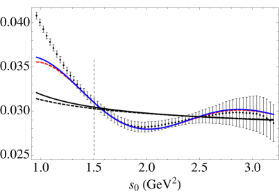
We observe that there is excellent stability for the results with , and GeV2, with the errors getting somewhat larger at 1.6 GeV2. At values of GeV2, becomes very small and tends to go negative, which is clearly unphysical. However, within errors such fits are always consistent with those shown in the table. We choose the results obtained at GeV2 to fix our central values, and treat the spread of the fit results for ranging from 1.4 to 1.6 GeV2 as an error. From this simple fit, we obtain for at the mass the values
| (21) | |||||
where the second error represents the variation with discussed above. We note that there is good stability over the full range of values covered in Table 1. Since our fitting function is non-linear, in general errors are expected to be asymmetric. We have therefore also computed asymmetric errors for all the fit parameters. We find that the error on is nearly symmetric, and that only errors on and show a significant asymmetry. For instance, we find, at GeV2, that, for FOPT,
| (22) | |||||
This shows that omitting DVs from the fit, which is equivalent to setting , would lead to a poor fit. For CIPT the asymmetries show the same pattern.
| 1 | -0.69 | -0.67 | 0.70 | -0.62 | |
| -0.69 | 1 | 0.99 | -0.47 | 0.43 | |
| -0.67 | 0.99 | 1 | -0.48 | 0.43 | |
| 0.70 | -0.47 | -0.68 | 1 | -0.98 | |
| -0.62 | 0.43 | 0.43 | -0.98 | 1 |
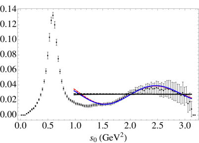
In Fig. 2, we show the quality of the match between the fitted and , as well as of the match between the experimental spectral function and its theoretical counterpart in which parameter values are obtained from the FESR fit for GeV2. The left panel shows the FESR fit itself, while the right panel shows the results of this comparison for the spectral function case. We emphasize that the spectral function was not part of the fit; the agreement between the theoretical and experimental versions of is an output. Agreement with data is good in the full fit window GeV2. The black curves, in contrast, show the OPE parts of the theoretical curves, i.e., the curves obtained by removing the DV contributions from the blue and red curves. It is clear that DVs are needed to give a good description of the data for and the spectral function itself, in agreement with our conclusion based on Eq. (22).
There are strong correlations between the parameters shown in Table 1 and Eq. (22). Such strong correlations are present in all our fits, and are unavoidable, given the number of fit parameters. We emphasize that this cannot be resolved by simply omitting the duality-violating part from the theory – one cannot “improve” fits by throwing out physics that is known to have an impact on those fits! In Table 2 we show the full parameter correlation matrix corresponding to the FOPT result quoted in Eq. (21). The analogous matrix for the CIPT result looks very similar.
We have also considered fits like those shown in Table 1, but including the contribution coming from the logarithmic dependence of on . For the latter, we estimated the quark-condensate contribution from the Gell-Mann–Oakes-Renner relation GMOR , and we took GeV4. We find that corresponding changes in the numbers in Table 1 are at most a tiny fraction of the fitting errors.
We performed a similar type of fit to the combination of and channels. If we use all possible values, we find that the standard fit function (involving the very strongly correlated spectral integral covariance matrix) is very flat, admitting not just “physical” solutions (consistent with those in Table 1), but also solutions that are clearly unphysical (with, for instance, values for drifting down to unacceptably low values as a function of ). This happens for both CIPT and FOPT. Parameter errors for these solutions can be very large, consistent with the flatness of the landscape, and there is a strong sensitivity of central values to initial guesses for the parameter values.
However, if we thin out the values i.e., use only every th value of , for some value of , we find that fits with , or are much more stable than the one with (no thinning) described above. In Table 3 we show our results for , which is the choice leading to the most stable fits.181818Negative values for can appear because we use the analytic form of the integral in Eq. (15). Note, however, that all values we find in the fits are consistent with a positive value, as physically required. The problem disappears when we use fit quality (18), computing errors with Eq. (43), but this method leads to significantly larger errors.
Choosing again the fit with GeV2, we find for our combined and channel fit the results
| (23) | |||||
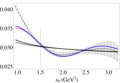
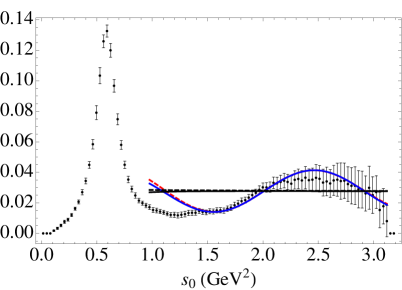
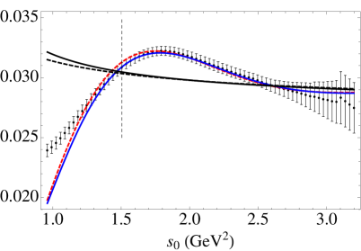
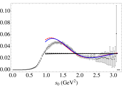
with the second error representing, as above, the variation over the neighboring values, and GeV2. The results reported in Tables 1 and 3 are in good agreement. We note that the central values for shown in Table 3 are very small, compared with those in Table 1, but given the errors there is no inconsistency. In Fig. 3 we show the quality of the fit in the panels on the left, for (top) and (bottom), for GeV2. In the panels on the right we show again the match between the experimental spectral functions and their theoretical counterparts with parameter values obtained from the GeV2 FESR fit. As before, black curves show only the OPE parts of the theoretical curves. Again, we see that the data clearly confirm the presence of DVs, which are well described by our ansatz.
| dof | /dof | ||||||
|---|---|---|---|---|---|---|---|
| 1.3 | 30 | 0.81 | |||||
| 1.4 | 28 | 0.69 | |||||
| 1.5 | 26 | 0.69 | |||||
| 1.6 | 24 | 0.73 | |||||
| 1.7 | 22 | 0.68 | |||||
| 1.3 | 30 | 0.85 | |||||
| 1.4 | 28 | 0.72 | |||||
| 1.5 | 26 | 0.71 | |||||
| 1.6 | 24 | 0.75 | |||||
| 1.7 | 22 | 0.70 | |||||
VI.2 Multiple-weight fits with the weights , and
One would naively expect that by using more moments, more information could be extracted from the data. This would help reducing the errors reported in Tables 1 and 3. Higher-degree weights, however, also require the introduction of additional OPE fit parameters. This, in combination with the very strong correlations, may turn out to reduce the extra constraints placed on the parameters ( and the DV parameters) entering the FESR by the additional moments. In addition, as we already pointed out in Sec. V.1, it appears to be impossible to perform standard fits to multiple moments.
Table 4 shows the results of simultaneous fits to moments with weights , , and for the channel using the fit quality (19), with errors computed from Eq. (43); see Fig. 4 for a visual representation of the qualities of the resulting fits for the case GeV2. Results are consistent with those presented in Sec. VI.1, but errors are slightly larger.
| dof | /dof | ||||||||
|---|---|---|---|---|---|---|---|---|---|
| 1.3 | 167 | 0.42 | |||||||
| 1.4 | 158 | 0.33 | |||||||
| 1.5 | 149 | 0.33 | |||||||
| 1.6 | 140 | 0.33 | |||||||
| 1.7 | 131 | 0.34 | |||||||
| 1.3 | 167 | 0.40 | |||||||
| 1.4 | 158 | 0.32 | |||||||
| 1.5 | 149 | 0.32 | |||||||
| 1.6 | 140 | 0.33 | |||||||
| 1.7 | 131 | 0.34 |
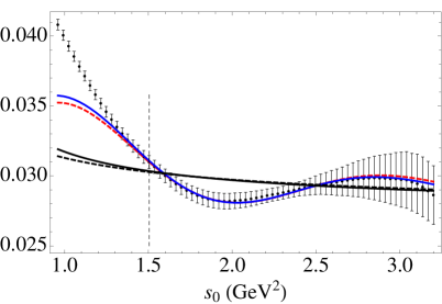
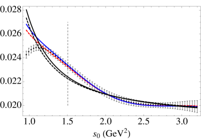
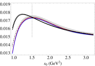
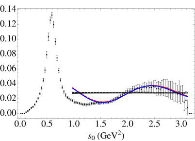
Again, the black curves in Fig. 4 show the OPE parts of the theoretical curves, i.e., the results obtained by removing the DV contributions from the blue and red curve results. For the spectral function, and , it is again clear that no good description of the data can be obtained without a model for DVs. This is not the case for the doubly-pinched moment . In this case, one would expect that a reasonably good fit can be obtained without DVs, for values of down to somewhere below GeV2. This is consistent with the results of Ref. MY for various doubly pinched weights, and, for the doubly pinched kinematic weight, also with the results of Refs. ALEPH ; OPAL ; in those cases, reasonably good matches for the sum of the vector and axial channels were obtained without the inclusion of DVs. However, one would also expect that a best fit can only be obtained by shifting the OPE parameters relative to those reported in Table 4.
An estimate similar to Eq. (21), using the fit with GeV2, leads to
| (24) | |||||
which is in excellent agreement with Eq. (21). We see, however, that the simultaneous fit to multiple moments does not help reduce the error. It is an interesting question whether fit qualities other than those of Eqs. (18) and (19) exist that would lead to smaller errors. Fits like those reported in Table 4 using fit quality (18) lead to consistent results, but with significantly larger errors than those shown in the table.
Finally, in Table 5, we show the results of combined channel fits, similar to those of Table 3, but for the weights , and . From this table, we obtain
| (25) | |||||
with the second error again reflecting the variation over the range to GeV2. Comparing Table 5 with Table 4 we see that adding the channel gives little extra information (apart from estimates of the axial OPE and DV parameters). Adding the channel increases the central values of , but all parameter values are consistent between these two tables within (sometimes substantial) errors. The fit with GeV2 is clearly not meaningful (in particular for FOPT), and the errors indicate that at this value of , is very flat in some directions in parameter space. Indeed, restricting the value of to the value obtained at GeV2 leads to a good fit for the remaining parameters, consistent with the unrestricted GeV2 fit, and with a value for almost equal to the value reported in the table.
| dof | /dof | ||||||||
|---|---|---|---|---|---|---|---|---|---|
| 1.3 | 104 | 0.66 | |||||||
| 1.4 | 98 | 0.48 | |||||||
| 1.5 | 92 | 0.47 | |||||||
| 1.6 | 86 | 0.46 | |||||||
| 1.7 | 80 | 0.41 | |||||||
| 1.3 | 104 | 0.55 | |||||||
| 1.4 | 98 | 0.45 | |||||||
| 1.5 | 92 | 0.45 | |||||||
| 1.6 | 86 | 0.41 | |||||||
| 1.7 | 80 | 0.42 | |||||||
Let us next deduce some implications of the above fits for the breaking of the factorization hypothesis in the condensates. To begin with, we will assume that the condensates are dominated by their leading-order contribution. The corresponding contribution to the correlators is given by BNP :
| (30) | |||||
|
|
where, in the first line, the upper Dirac structure corresponds to the channel and the lower to the channel. The two four-quark condensates can be parametrized in terms of their factorization values by
| (31) | |||||
where the parameters and would be equal to one if the vacuum-saturation approximation were exact. Further assuming that isospin breaking is small in the light - and -quark sector, that is , Eqs. (30) and 31 imply
| (32) |
Inverting Eq. (32), on the basis of the results of Table 5, estimates of the parameters can be deduced. As representative examples, for the central fits with GeV2, one obtains:
| (33) | |||||
where jam02 ,
together with our results for , has been employed. The
central results of Eq. (33) display sizable deviations from the
factorization values , though, given the large uncertainties,
the significance is not very high. The employed perturbative resummation scheme
does not seem to play a big role for the condensate or DV parameters, suggesting
that this choice is mostly compensated for by the differing values.
VI.3 Errors from truncating perturbation theory
One of the uncertainties afflicting any determination of is that perturbation theory needs to be truncated, irrespective of whether the CIPT or FOPT resummation scheme is used for the truncated series. As already mentioned in Sec. II, we use the known values of up to , together with the estimate . We assign a error, , to this estimate, using this as a measure of the truncation uncertainty.
VI.4 Consistency with the and chiral sum rules
While Figs. 2–4 show that the parameter values obtained from the fits corresponding to these figures give a good description of the data, with those parameter values in hand one may also consider other quantities. The total non-strange scaled branching fraction (cf. Eqs. (6), (8) and (20)) has always played a central role in the study of hadronic decays. In particular, following Refs. ALEPH ; OPAL , we may consider for a hypothetical of mass-squared , as a function of . We show our version of this quantity in Fig. 5, using the parameter values for the fit with GeV2 of Table 5, the only fit reported that simultaneously yields all parameters needed to evaluate .191919We included the pion-pole contribution to the longitudinal part in Eq. (8) in both the data points and the theory curves in Fig. 5. Clearly, our result compares well with the fits shown in Fig. 10 of Ref. OPAL ,202020For an early investigation of this type, see Ref. GN . especially keeping in mind that in Fig. 5 we only show errors on the experimental spectral integrals, and not on the theory curves. Both CIPT and FOPT describe the data well down to GeV2. We used the same values for and as Ref. OPAL in order to plot . In view of the discussion in Ref. MY of the analysis of Refs. ALEPH ; OPAL , we conclude that our fits pass the test of much better than the original analyses of Refs. ALEPH ; OPAL , and over a wider range of than the alternate, self-consistent fits obtained ignoring DVs in Ref. MY . We emphasize, though, that it is not sufficient to find a satisfactory description of this quantity only – at the very least all FESRs used in the fits should show a similarly good match between experiment and theory as a function of , as was shown to be the case for our fits in Secs. VI.1 and VI.2 above.
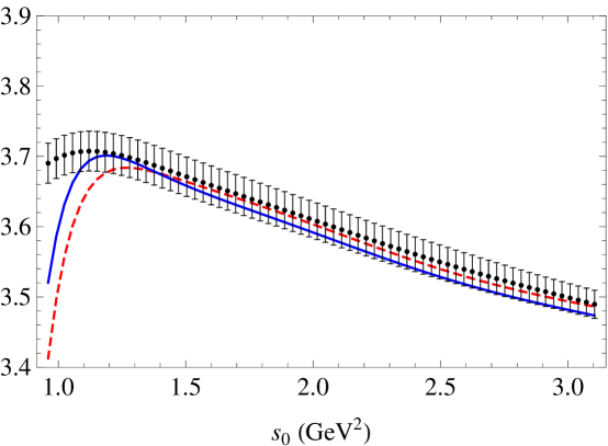
We may perform a similar test on the fits reported in Table 4. Of course, in that case only -channel parameters are available, so one should consider the corresponding ratio as a function of . For the channel, coincides (up to the overall factor ) with . The corresponding match between data and theory for GeV2 is shown in the left bottom panel of Fig. 4.
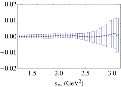
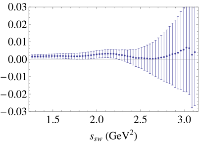
We can also test our results by considering how well they satisfy the classical chiral sum rule constraints represented by the two Weinberg sum rules SW and the DGMLY sum rule for the electromagnetic mass splitting EMpion . These tests focus specifically on the DV part of our spectral functions, since the OPE for the correlator (and hence the OPE part of the spectral ansatz) has no contribution and OPE contributions to are tiny, and can be ignored.
Weinberg’s sum rules can be written as
| (34) | |||||
where we assumed, as before, that we can neglect terms of order with , even though there is a term of order linearly divergent in in the second sum rule. The fact that this term is still very small at amounts to the observation that the chiral symmetry breaking terms in the second of Eq. (34) are not visible in the data. This means that in our test of the second sum rule we can assume ourselves to be effectively in the chiral limit, in which the divergence does not appear. In Fig. 6 we show the integrals in Eq. (34) as a function of the “switch point” below which experimental spectral data is used and above which the difference of the and DV ansätze of Eq. (16) is employed for . The DV contributions were obtained using the DV parameter values of Table 5. If the DV ansatz is, as we have assumed, reliable in the window of employed in the FESR fits which produce these DV parameter values, the sum rules should be satisfied for all values of lying in this fit window. We see that this condition is well satisfied for both of the Weinberg sum rules. The errors shown are those from the experimental () part of the integral on the left-hand side of the sum rules only.
The first Weinberg sum rule is, of course, closely related to the difference of the and FESRs. Therefore, the very good quality of the matches between the experimental spectral integrals and our theoretical representations thereof precludes the first Weinberg sum rule being badly broken by our fits. The second Weinberg sum rule (as well as the DGMLY sum rule discussed below) can be viewed as a prediction, because the fits of Table 5 do not involve any weight with a term linear in . We also note that if indeed we take the second sum rule in the chiral limit, we should omit the term . The value of this term is GeV4, and it can thus indeed safely be dropped from the sum rule — the difference would not be visible in the figure.
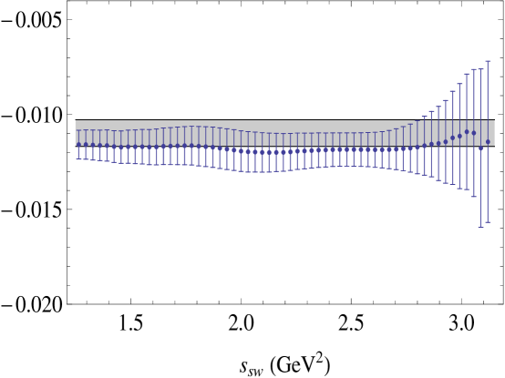
Finally, we consider the DGMLY sum rule for the electromagnetic mass difference. To leading order in the chiral expansion, one has that
| (35) |
where is the fine-structure constant, and the decay constant in the two-flavor chiral limit. On the right-hand side we take as input the values MeV MILC and GeV2 PDG .212121Our uncertainty on the electromagnetic contribution to the difference comes from an estimate of the contribution of to the pion mass difference ABT . Because of the second Weinberg sum rule, the left-hand side of Eq. (35) is, in fact, independent of the scale . In Fig. 7 we show the left-hand and the right-hand sides of Eq. (35), as a function of . The left-hand side is represented by the data points, while the gray band represents the right-hand side, including the error resulting from the uncertainties in and the pion electromagnetic mass difference. As for the Weinberg sum rules, the integral on the left-hand side is computed using experimental data for , and the DV ansatz, with DV parameters from the GeV2 entries of Table 5, for . The errors shown again come from the experimental data part of the integral only. We chose GeV2, which makes the errors in the figure relatively small. For lower values of the errors are larger for larger , but the results are consistent with Eq. (35) being satisfied for all between GeV2 and .
One might consider using these sum rules as a further constraint on the DV parameters.222222See, for instance, Ref. VAVal , where, however, the difference was modeled with an expression of the form (16). Given the results of Tables 3 and 5, such a parametrization does not seem to be favored by the data. In the present work we avoid any additional assumptions about the relations between the DV parameters in the and channels by introducing separate DV parameters for each channel. Of course, this can only be done for combined fits, which requires us to assume that the larger of the two values for the and channels still lies sufficiently far below to make such a combined fit, using our DV ansatz in both channels, reliable. Since in this work our primary results are obtained from purely -channel fits, which do not require this assumption, we postpone this possibility to a future investigation.
VII Summary of results
Our most stable results come from fits to only the channel. Moreover, since we need to include a model for DVs, using only the channel avoids the additional assumption that our ansatz already adequately describes the -channel data in the interval between GeV2 and . We emphasize, however, that all the results from our combined and channel fits are consistent with those from our -channel analyses. In addition, they pass several further and channel tests, as demonstrated in Sec. VI.4.
In view of these observations, we will choose the fit to in the vector channel as our central result. Adding the errors from the fit, the variation of and the variation of in quadrature, we find
| (36) | |||||
We do not average over CIPT and FOPT results, because we believe that it is useful to see the difference between values for obtained with the two resummation schemes after all non-perturbative effects have been consistently taken into account. Running these values up to the mass yields CKS 232323 The specifics of the evolution to the mass are as discussed in Ref. BJ .
| (37) | |||||
where we symmetrized the slightly asymmetric errors one obtains after running up to the mass.
These values can be compared to those obtained by OPAL from the same data OPAL . The OPAL values at the mass are
| (38) | |||||
where we added the experimental and theoretical errors quoted by OPAL in quadrature. We observe the shift to lower central values, with somewhat larger errors that follow from using our new framework for analyzing the data. We also note that our CIPT and FOPT values are somewhat closer, and that, because of the larger errors, the difference between our two values for is less significant.
VIII Conclusion
In this article, we provided a new framework for the extraction of and other OPE parameters from hadronic decays. This new framework combines two elements that have not been taken into account in the “traditional” analysis of hadronic decays. One is a consistent treatment of the OPE, as discussed in Ref. MY , and the other is a detailed quantitative estimate of the effect of violations of quark-hadron duality, using a parametrization proposed in Refs. CGPmodel ; CGP05 . As explained in detail in Secs. III and IV, these two elements are intricately intertwined.
Our new framework comes with the price of introducing four new fit parameters for each channel, the vector and axial-vector DV parameters. Nevertheless, we demonstrated that our method is feasible by presenting a rather complete analysis based on the OPAL data for the and spectral functions OPAL . With the larger number of parameters, and the corresponding need to vary away from , it should come as no surprise that our errors are typically larger than those found in earlier analyses, which simply did not take DVs into account quantitatively. We emphasize that this means that the systematic errors of those earlier analyses were understimated – we believe significantly so in some cases.
Our analysis leads us to a new estimate for both the central value of and the error, which, in our opinion, should be interpreted as superseding previous estimates in the literature; for our result, based on OPAL data, see Sec. VII. We found our most reliable fits to be those of the channel, although fits including also the channel lead to results consistent with our most precise -channel fits. As our primary concern in this article is with previously underestimated non-perturbative effects, we presented results for both contour-improved as well as fixed-order perturbation theory. Our analysis was based on the original OPAL data, unmodified for subsequent changes in the various exclusive branching fractions. This choice was made in order to facilitate interpretation of the differences in our results from those obtained by OPAL. With this choice, these differences are solely the result of differences in the analysis method. We plan to present an analysis of OPAL data with updated normalizations in the near future.
The accuracy of the results presented here depends in part on our ability to correctly model the physics present in duality violations. Conservatively, our results can be seen as providing a lower bound on the error introduced by ignoring duality violations. However, the stability of , a purely perturbative parameter, across the range of moments analyzed here provides strong support for the validity of our ansatz. We therefore surmise that not only is the ansatz able to accurately describe the data, but also that it provides a reasonable quantitative description of the physics of duality violations in the light-quark and channels.
In cases with multiple weights, standard fits were not possible, and we performed alternate fits, propagating errors as described in App. A. We point out, however, that our final result is based on a standard fit to the moment . All other fits yield results completely consistent with this result, including the error on . The error on obtained from our fit to is very close to that obtained with the method of App. A. Because our parameter covariance matrix obtained with that method scales linearly with the data covariance matrix, the error on will be reduced once the improved spectral function data expected from BaBar and/or Belle becomes available.
We observe that a difference remains between the central values for obtained using CIPT and FOPT, though this is less significant than the difference found previously by OPAL, cf. Eq. (38). In this context, we note that, as mentioned already in Sec. IV.1, a term linear in in any of the weights employed in Eq. (4) picks out the term in the OPE, which parametrizes the leading renormalon ambiguity in the perturbative expansion. This, then, raises the question whether differences between the behavior of CIPT and FOPT fits, including those associated with any dependence on the choice of weight, might be used to constrain renormalon pole models that have been used previously to investigate the resummation of the perturbative series for the various sum rules employed in the study of hadronic decays BJ ; DM . We plan to pursue such an investigation in a future work.
Acknowledgments
We would like to thank Martin Beneke, Claude Bernard, Andreas Höcker, Manel Martinez, and Ramon Miquel for useful discussions. We also would like to thank Sven Menke for significant help with understanding the OPAL spectral-function data. MG thanks IFAE and the Department of Physics at UAB, and OC and KM thank the Department of Physics and Astronomy at SFSU for hospitality. DB, MJ and SP are supported by CICYTFEDER- FPA2008-01430, SGR2005-00916, the Spanish Consolider-Ingenio 2010 Program CPAN (CSD2007-00042). SP is also supported by a fellowship from the Programa de Movilidad PR2010-0284. OC is supported in part by MICINN (Spain) under Grant FPA2007-60323, by the Spanish Consolider Ingenio 2010 Program CPAN (CSD2007-00042) and by the DFG cluster of excellence “Origin and Structure of the Universe.” MG and JO are supported in part by the US Department of Energy, and KM is supported by a grant from the Natural Sciences and Engineering Research Council of Canada.
Appendix A Error propagation
Consider a fit quality
| (39) |
in which are the binned data, is a function that describes this data set for a set of parameters , and is a positive-definite, symmetric, but otherwise arbitrary matrix. In this Appendix, we use the summation convention for repeated indices. The parameters are determined by finding the global minimum of , which satisfies
| (40) |
Varying, in this equation, the data by an amount , and the parameters by leads to
| (41) |
If the fit is good, so that the deviations are small, we may ignore the term with the second derivative, leading to
| (42) |
or, for the covariance matrix ,
| (43) |
in which
| (44) |
and
| (45) |
is the data covariance matrix. This provides us with an estimate for the full correlation matrix for the parameter set . We note that, if is chosen to be equal to the data covariance matrix , this expression simplifies to
| (46) |
This is equal to the usual error matrix estimate, given by the inverse of one-half times the second derivative of at its minimum, if, again, the fit is good enough to ignore terms proportional to .
References
- (1)
- (2) P. A. Baikov, K. G. Chetyrkin and J. H. Kühn, Phys. Rev. Lett. 101, 012002 (2008) [arXiv:0801.1821 [hep-ph]].
- (3) E. Braaten, S. Narison, and A. Pich, Nucl. Phys. B 373 581 (1992).
- (4) S. Bethke, Eur. Phys. J. C64, 689 (2009) [arXiv:0908.1135 [hep-ph]].
- (5) R. Barate et al. [ALEPH Collaboration], Eur. Phys. J. C4, 409 (1998).
- (6) S. Schael et al. [ALEPH Collaboration], Phys. Rept. 421, 191 (2005) [arXiv:hep-ex/0506072].
- (7) K. Ackerstaff et al. [OPAL Collaboration], Eur. Phys. J. C 7, 571 (1999) [arXiv:hep-ex/9808019].
- (8) M. Davier et al., Eur. Phys. J. C56, 305 (2008) [arXiv:0803.0979 [hep-ph]].
- (9) M. Beneke and M. Jamin, JHEP 0809, 044 (2008) [arXiv:0806.3156 [hep-ph]].
- (10) S. Menke, arXiv:0904.1796 [hep-ph].
- (11) I. Caprini and J. Fischer, Eur. Phys. J. C 64, 35 (2009) [arXiv:0906.5211 [hep-ph]]; I. Caprini and J. Fischer, Phys. Rev. D84, 054019 (2011), [arXiv:1106.5336 [hep-ph]].
- (12) S. Descotes-Genon, B. Malaescu, arXiv:1002.2968 [hep-ph].
- (13) K. Maltman, T. Yavin, Phys. Rev. D78, 094020 (2008) [arXiv:0807.0650 [hep-ph]].
- (14) O. Catà, M. Golterman, S. Peris, Phys. Rev. D79, 053002 (2009) [arXiv:0812.2285 [hep-ph]].
- (15) D. R. Boito, O. Catà, M. Golterman, M. Jamin, K. Maltman, J. Osborne, S. Peris, Nucl. Phys. Proc. Suppl. 218, 104 (2011) [arXiv:1011.4426 [hep-ph]].
- (16) S. Weinberg, Phys. Rev. Lett. 18, 507 (1967).
- (17) T. Das, G. S. Guralnik, V. S. Mathur, F. E. Low, J. E. Young, Phys. Rev. Lett. 18, 759 (1967).
- (18) R. Shankar, Phys. Rev. D15, 755 (1977); R. G. Moorhose, M. R. Pennington and G. G. Ross, Nucl. Phys. B124, 285 (1977); K. G. Chetyrkin and N. V. Krasnikov, Nucl. Phys. B119, 174 (1977); K. G. Chetyrkin, N. V. Krasnikov and A. N. Tavkhelidze, Phys. Lett. 76B, 83 (1978); N. V. Krasnikov, A. A. Pivovarov and N. N. Tavkhelidze, Z. Phys. C19, 301 (1983); E. G. Floratos, S. Narison and E. de Rafael, Nucl. Phys. B155, 115 (1979); R. A. Bertlmann, G. Launer and E. de Rafael, Nucl. Phys. B250, 61 (1985).
- (19) Y. -S. Tsai, Phys. Rev. D4, 2821 (1971).
- (20) K. Nakamura et al. (Particle Data Group), J. Phys. G37, 075021 (2010).
- (21) M. Jamin, JHEP 0509, 058 (2005) [hep-ph/0509001].
- (22) A. A. Pivovarov, Z. Phys. C 53, 461 (1992) [Sov. J. Nucl. Phys. 54, 676 (1991)] [Yad. Fiz. 54 (1991) 1114] [arXiv:hep-ph/0302003]; F. Le Diberder, A. Pich, Phys. Lett. B286, 147 (1992).
- (23) S. Narison, V. I. Zakharov, Phys. Lett. B679, 355 (2009) [arXiv:0906.4312 [hep-ph]].
- (24) K. G. Chetyrkin, V. P. Spiridonov, S. G. Gorishnii, Phys. Lett. B160, 149 (1985); A. Pich, J. Prades, JHEP 9910, 004 (1999) [hep-ph/9909244].
- (25) M. S. Dubovikov, A. V. Smilga, Nucl. Phys. B185, 109 (1981); W. Hubschmid, S. Mallik, Nucl. Phys. B207, 29 (1982).
- (26) L. V. Lanin, V. P. Spiridonov, K. G. Chetyrkin, Sov. J. Nucl. Phys. 44, 812 (1986) [Yad. Fiz. 44, 1372 (1986)]; L. E. Adam, K. G. Chetyrkin, Phys. Lett. B329, 129 (1994) [hep-ph/9404331].
- (27) E. C. Poggio, H. R. Quinn, S. Weinberg, Phys. Rev. D13, 1958 (1976).
- (28) O. Catà, M. Golterman, S. Peris, Phys. Rev. D77, 093006 (2008) [arXiv:0803.0246 [hep-ph]].
- (29) B. Blok, M. A. Shifman and D. X. Zhang, Phys. Rev. D 57, 2691 (1998) [Erratum-ibid. D 59, 019901 (1999)] [arXiv:hep-ph/9709333]; I. I. Y. Bigi, M. A. Shifman, N. Uraltsev, A. I. Vainshtein, Phys. Rev. D59, 054011 (1999) [hep-ph/9805241]; M. A. Shifman, [hep-ph/0009131]; M. Golterman, S. Peris, B. Phily, E. de Rafael, JHEP 0201, 024 (2002) [hep-ph/0112042].
- (30) O. Catà, M. Golterman, S. Peris, JHEP 0508, 076 (2005) [hep-ph/0506004].
- (31) M. Jamin, JHEP 1109, 141 (2011), [arXiv:1103.2718 [hep-ph]].
- (32) F. Le Diberder, A. Pich, Phys. Lett. B289, 165 (1992).
- (33) S. Narison, Phys. Lett. B673, 30 (2009) [arXiv:0901.3823 [hep-ph]].
- (34) M. Jamin, Phys. Lett. B538, 71 (2002) [hep-ph/0201174].
- (35) K. Maltman, Phys. Lett. B440, 367 (1998) [hep-ph/9901239]; C. A. Dominguez, K. Schilcher, Phys. Lett. B448, 93 (1999) [hep-ph/9811261].
- (36) M. Gell-Mann, R. J. Oakes, B. Renner, Phys. Rev. 175, 2195 (1968).
- (37) M. Gonzalez-Alonso, A. Pich, J. Prades, Phys. Rev. D82, 014019 (2010) [arXiv:1004.4987 [hep-ph]]; Phys. Rev. D81, 074007 (2010) [arXiv:1001.2269 [hep-ph]].
- (38) M. Girone, M. Neubert, Phys. Rev. Lett. 76, 3061 (1996) [hep-ph/9511392].
- (39) A. Bazavov, et al. [MILC Collaboration], PoS LATTICE2010, 074 (2010) [arXiv:1012.0868 [hep-lat]].
- (40) G. Amoros, J. Bijnens, P. Talavera, Nucl. Phys. B602, 87 (2001) [hep-ph/0101127].
- (41) K. G. Chetyrkin, B. A. Kniehl, M. Steinhauser, Phys. Rev. Lett. 79, 2184 (1997) [hep-ph/9706430].