A simple method to estimate radial velocity variations due to stellar activity using photometry

Abstract

We present a new, simple method to predict activity-induced radial velocity variations using high-precision time-series photometry. It is based on insights from a simple spot model, has only two free parameters (one of which can be estimated from the light curve) and does not require knowledge of the stellar rotation period. We test the method on simulated data and illustrate its performance by applying it to MOST/SOPHIE observations of the planet host-star HD 189733, where it gives almost identical results to much more sophisticated, but highly degenerate models, and synthetic data for the Sun, where we demonstrate that it can reproduce variations well below the m s^-1 level. We also apply it to Quarter 1 data for Kepler transit candidate host stars, where it can be used to estimate RV variations down to the 2–3 m s^-1 level, and show that RV amplitudes above that level may be expected for approximately two thirds of the candidates we examined.

1 Introduction

Stellar activity induces brightness and line-shape variations which can mimic planetary signals and hinder the detection and/or characterisation of the latter. In particular, in radial velocity (RV) surveys, many stars display intrinsic variability which is attributed to activity, and which occurs on timescales similar to the planetary signals of interest. There is thus significant interest in characterising the level of activity-induced RV variability in stars targeted by planet surveys, and in developing tools to distinguish between the latter and planetary signals.

The simplest, widely used method to deal with activity-induced variability in RV surveys is to add a ‘jitter’ term in quadrature to the RV uncertainties before searching for planetary signals. Wright (2005) proposed an empirical relation to predict the magnitude of this jitter term from a star’s activity level, $B-V$ colour and absolute magnitude, calibrated on 450 targets from the California and Carnegie planet search, but this relation is far from tight. More recently, Isaacson & Fischer (2011) determined chromospheric activity levels for over 2500 target stars from the same survey, and compared them to the RMS scatter of their RV variations. Again, there is clearly a relationship between the two – in particular, the lower envelope of the RV scatter increases for increasing levels of activity – but there is also a wide range of RV scatters for a given spectral type and activity level. Furthermore, the ‘jitter’ formalism is limited, because it treats the activity signal as an independent, identically distributed Gaussian noise process. Activity-induced RV signals arise from the rotational modulation and intrinsic evolution of magnetized regions, and are thus naturally correlated in time, often quasi periodic, and non-stationary. Therefore the impact of variability-induced RV signals on planet detection will generally be much more severe than that of a random “jitter” of the same mean amplitude.

For individual stars, somewhat more sophisticated approaches are in common use, mostly making use of chromospheric activity indicators, such as excess flux in the cores of the H$\alpha$ and Ca ii H & K lines, of measurements of the degree of asymmetry of the spectral lines, such as the bisector span of the cross-correlation function (CCF) between the stellar spectrum and a template, which is often used to derive the RV itself. The most obvious step is to check for periodic modulation in these indicators, which can reveal that a suspected planetary signal is in fact due to activity (see e.g. Queloz et al., 2001; Bonfils et al., 2007). The correlation between RVs and bisector span can also be used to correct for the effect of activity at the few m s^-1 level (Melo et al., 2007; Boisse et al., 2009). However, this correlation is highly dependent on the spot distribution and stellar inclination (Boisse et al., 2011) and is not always present. In Pont et al. (2011), we developed another method, which consists in modeling the variations of the stellar brightness and the CCF bisector span using a spot model, to predict the activity-induced variations. Spot models are very degenerate: many spot distributions with widely different numbers of spots and spot parameters fit the data equally well, so the predictions of many models must be averaged. One way to address this degeneracy is to use maximum entropy regularisation, as was done by Lanza et al. (2007), to model the Sun’s total irradiance variations. Recently, Lanza et al. (2011) applied this method to the planet-host star HD 189733, using photometric observations performed by the MOST satellite to predict the activity signal in simultaneous SOPHIE RV observations, and obtained slightly better results than Boisse et al. (2009), who had previously analysed the same dataset using the bisector span de-correlation method.

The data from space-based transit surveys such as CoRoT and Kepler contain a wealth of information about stellar activity, but the spot-modeling approaches above are computationally intensive to be applied systematically to many light curves. They are also dependent on fairly detailed a-priori knowledge of the star being modeled, and in particular of its rotation period. In this paper, we present a new, much simpler method to predict the activity-induced RV variations for a given star from its photometric variations, which can be applied to stars whose rotation period is not known. This is intended primarily for statistical purposes: to characterise the overall RV variability properties of a sample of stars, and to select the best targets for RV follow-up, for example. However, as Kepler continues to observe the candidate planets it has identified while they are being followed up from the ground, our method may also prove useful in reducing contamination of the RV data by activity signals in individual cases.

Our method is based on a very simple spot model, which we introduce in Section 2. We then make use of a relationship between the photometric and RV signatures of individual spots to formulate a means of simulating the RV variations based on the light curve only, as outlined in Section 3. In Section 4, we test the method on simulated data and give three example applications: the SOPHIE/MOST observations of HD 189733b already used as a test case by Boisse et al. (2009) and Lanza et al. (2011), total irradiance and RV variations of the Sun synthesized by Meunier et al. (2010b), and Kepler quarter 1 light curves for a subset of the planetary candidates published by Borucki et al. (2011). We present our conclusions and future plans for applying the method to other datasets, in Section 5.

2 A simple spot model

Dorren (1987) provided analytic expressions to model the photometric signature of a circular spot on a rotating stellar surface, accounting for limb-darkening using a single-coefficient, linear limb-darkening law. It is possible to expand these to also model the RV signature of such a spot, and to account for both dark spots and bright faculae by allowing the contrasts and limb-darkening coefficients to change sign. However, the resulting algebra is relatively cumbersome. Here we seek a simpler model, whose mathematical expressions are simple enough to afford a more direct insight into the dependency of the photometric and RV signatures of active regions on the various parameters, while retaining as much realism as possible. In order to achieve this, we make a number of simplifications, the impact of which we will test by comparing our results to data simulated using the more complete Dorren (1987) formalism.

2.1 Photometric signature of a point-like spot

To model the photometric signature of dark spots, we assume that the spots are small, i.e. that $\alpha\ll 1$, where $\alpha$ is the spot’s angular radius on the surface of the star. This allows us to ignore projection effects within a spot, and obviates the need to assume a particular shape for the spots. It also enables us, when considering multiple spots, to assume that they never overlap. Additionally, we ignore limb-darkening. This alters the photometric signature of dark spots only slightly, since both the spot and the un-spotted photosphere are darker towards the limb than they are near the centre of the stellar disk.

Under these conditions, the relative drop in flux due to a single point-like, dark spot rotating on the stellar surface is

$$F(t)=f~{}{\rm MAX}\left\{\cos\beta(t);0\right\},$$ (1)

where $f=2(1-c)(1-\cos\alpha)$ represents the relative flux drop for a spot at the disk centre, $c$ is the contrast ratio between the spot and the un-spotted photosphere, and $\beta(t)$ is the angle between the spot normal and the line of sight. This angle is given by

$$\cos\beta(t)=\cos\phi(t)\,\cos\delta\,\sin i+\sin\delta\cos i,$$ (2)

where $i$ is the stellar inclination (the angle between the star’s rotation axis and the line of sight), $\delta$ is the latitude of the spot relative to the star’s rotational equator, and $\phi(t)$ is the phase of the spot relative to the line of sight (see Appendix A for details). The latter is of course $\phi(t)\equiv 2\pi t/P_{\rm rot}+\phi_{0}$, where $P_{\rm rot}$ is the star’s rotation period and $\phi_{0}$ is the longitude of the spot (i.e. we take the stellar meridian to be aligned with the line of sight at $t=0$). The observed stellar flux is then simply

$$\Psi(t)=\Psi_{0}\left[1-F(t)\right],$$ (3)

where $\Psi_{0}$ is the flux in the absence of spots.

By allowing $c$ to exceed one, one could use the equations above to model the signature of bright spots such as faculae. However, faculae on the Sun are limb-brightened (see e.g. Lanza et al., 2007; Meunier et al., 2010a, and references therein), and any model that ignores the limb-angle dependence of the contrast will not reproduce their photometric signature well. Thus we have opted not to include faculae in our model. Fortunately, the latter typically have low contrast, and hence the missing photometric effect tends to be small. Comparative studies of Sun-like stars by Radick et al. (1998) and Lockwood et al. (2007) also suggest that faculae are less important in stars more active than the Sun.

2.2 RV signature

The most important effect of the spot in RV is due to the fact that it suppresses the flux emitted by a portion of the rotating stellar disk, thus introducing a perturbation to the disk-averaged RV. Provided $c$ is not close to one, this perturbation can be estimated simply by multiplying the projected area of the spot, which is given by $F(t)$, by the RV of the stellar surface at the location of the spot:

$$\Delta RV_{\rm rot}(t)=-F(t)\,V_{\rm eq}\,\cos\delta\sin\phi(t)\,\sin i,$$ (4)

where $V_{\rm eq}=2\pi R_{\star}/P_{\rm rot}$ is the equatorial rotational velocity of the star, and $R_{\star}$ the stellar radius. Differential rotation can be included in this formalism by allowing $V_{\rm eq}$ (or equivalently $P_{\rm rot}$) to vary as a function of the spot latitude.

Spots tend to be associated with magnetized areas which, while they have very limited photometric contrast, are much more extended spatially. These do have an important impact in RV, because convection is partially suppressed within them, leading to a reduction in the convective blue-shift (see Meunier et al., 2010a, b, and references therein). Within our simplified formalism, it is possible to approximate the resulting RV perturbation as

$$\Delta RV_{\rm c}(t)=+F(t)\,\delta V_{\rm c}\,\kappa\,\cos\beta(t)$$ (5)

where $\delta V_{\rm c}$ is the difference between the convective blue-shift in the unspotted photosphere and that within the magnetized area, and $\kappa$ is the ratio of this area to the spot surface (typically $\gg 1$). The total RV signature of the spot and associated magnetised area is then simply

$$\Delta RV(t)=\Delta RV_{\rm rot}(t)+\Delta RV_{\rm c}(t).$$ (6)

2.3 Examples

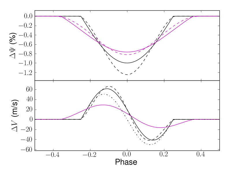
Figure 1: Simulated photometric and RV signatures of a single spot (top and bottom respectively). The solid black line shows the output of our simple model for a fairly large, dark, equatorial spot ($c=0$, $\alpha=10\,^{\circ}$, $\delta=0$) on a star with $P_{\rm rot}=5$ days, $i=90\,^{\circ}$, $\delta V_{\rm c}=200$ m s^-1 and $\kappa=10$ (see text for details). The solid cyan line is the same, but for a higher latitude spot on an inclined star ($\delta=60\,^{\circ}$, $i=70\,^{\circ}$). For comparison, the dashed lines show the same spots modeled with the formalism of Dorren (1987) (stellar linear limb-darkening parameter $u_{\star}=0.5$). For simplicity, we have omitted the Dorren formalism for the high-latitude case in the bottom panel. Instead, the black dash-dot line shows the equatorial spot simulated with our simple model, but without the convective blue-shift effect ($\delta V_{\rm c}=0$).

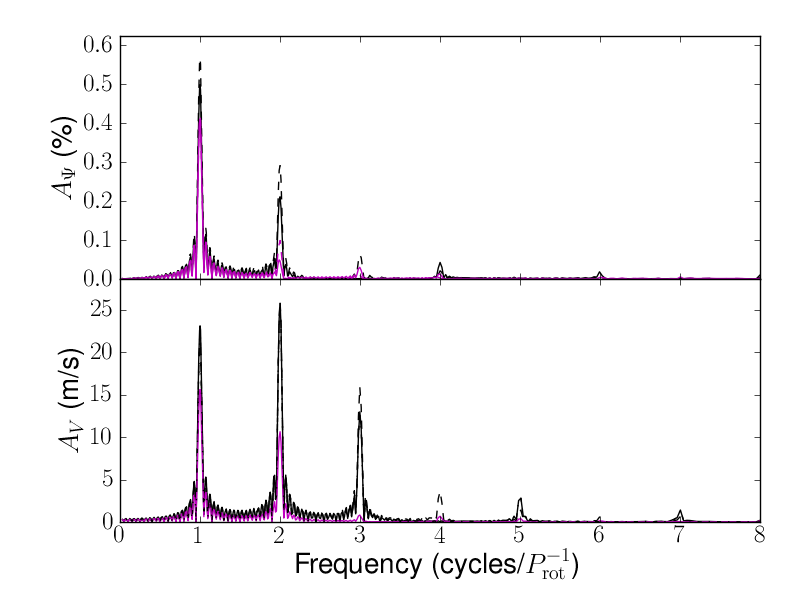
Figure 2: Amplitude spectra for the light and RV curves shown in 1, using the same colour-coding. These spectra were computed from time-series lasting $5\,P_{\rm rot}$. Frequencies are expressed in units of inverse rotation periods.

Figure 1 shows light and RV curves simulated using this simple model for an equatorial spot (solid black line) and a high-latitude spot on an inclined star (solid cyan line). The dotted grey line in the bottom panel shows the equatorial spot case without the convective blue-shift suppression term. Also shown for comparison is the same equatorial spot modeled with the more sophisticated formalism of Dorren (1987), who gives analytical expressions for a circular spot of finite size on a limb-darkened photosphere. Figure 2 shows the corresponding amplitude spectra, which we use to evaluate the impact of the simplifications we have made on the frequency content of the simulated light and RV curves.

In all cases, the amplitude spectrum of the light curve is dominated by the rotational frequency, as one might expect. There is also signal at the second, fourth, sixth and higher even-numbered harmonics $\nu=2n/P_{\rm rot}$, where $n=1,2,3$,…, although the amplitude decreases rapidly with $n$. On the other hand, there is essentially no signal at odd-numbered harmonics $\nu=(2m+1)/P_{\rm rot}$, where $m=1,2,3$,…. As previously noted by Boisse et al. (2009, 2011), the RV signature is dominated by the first three harmonics of the rotational frequency, with additional signal at odd-numbered harmonics, although at much lower amplitude. The differences between the distribution of power at higher harmonics in photometry and in RV arise because the photometric signal is maximised when the spot is face on, which occurs once per disk-crossing, but the RV signal is maximised when the spot longitude is $45^{\circ}$, which occurs twice per disk crossing.

Changing the spot latitude and stellar inclination can substantially alter the light and RV curves, as it changes the fraction of the rotation cycle over which the spot remains in- or out-of-view, and the rotational velocity of the occulted parts of the stellar disk. This results in significant changes in the relative amounts of power at the different harmonics of the rotational frequency, in some cases entirely suppressing all but the fundamental, or on the contrary giving rise to relatively large amplitudes at high-$n$ harmonics. Projection effects over the area of the spot, and limb-darkening (both of which are accounted for in the Dorren 1987 formalism, but not in our simple model), alter the shape and maximum amplitude of the light curve, and hence the balance of power between the fundamental and second harmonic, but not in a very substantial way (except for extremely large spots). The effect on the RV signature is even smaller.

The convective blue-shift causes the RV perturbation to be biased upwards and to depart from an exact sinusoidal shape. As $\Delta RV_{\rm c}(t)$ is proportional to $F^{2}$, the power of the convective component of the RV signature is concentrated at the rotational frequency and its first harmonic. Except for extreme cases, the effect of convective blue-shift on the frequency content of the RV curve remains minor.

3 The $FF^{\prime}$ method

3.1 Relationship between photometric and RV signatures

Considering the equations of our spot model, as presented in Section 2, it is interesting to note that

$$\dot{F}(t) = -f\,\sin\phi(t)\,\dot{\phi}(t)\,\cos\delta\,\sin i$$ (7)

$$= -f\,\sin\phi(t)\,\cos\delta\,\sin i\,\frac{2\pi}{P_{\rm rot}}.$$

Therefore the expression for the RV signature of spots can be re-written:

$$\Delta RV_{\rm rot}(t)=-F(t)\,\dot{F}(t)\,R_{\star}/f.$$ (8)

This can be estimated directly from the light curve, as

$$F(t)=1-\frac{\Psi(t)}{\Psi_{0}}\hskip 28.45274pt{\rm and}\hskip 28.45274pt\dot{F}(t)=-\frac{\dot{\Psi}(t)}{\Psi_{0}},$$ (9)

hence

$$\Delta RV_{\rm rot}(t)=\frac{\dot{\Psi}(t)}{\Psi_{0}}\,\left[1-\frac{\Psi(t)}{\Psi_{0}}\right]\,\frac{R_{\star}}{f}.$$ (10)

Similarly, the convective blue-shift effect is given by

$$\Delta RV_{\rm c}(t)=+F^{2}(t)\,\delta V_{\rm c}\,\kappa/f,$$ (11)

which can be estimated from the light curve as

$$\Delta RV_{\rm c}(t)=+\left[1-\frac{\Psi(t)}{\Psi_{0}}\right]^{2}\,\frac{\delta V_{\rm c}\,\kappa}{f}.$$ (12)

The above expressions provide a means to simulate activity-induced RV variations based on a well-sampled light curve, without knowing the rotation period. As this method uses the light curve and its own derivative, we refer to it as the $FF^{\prime}$ method.

The effect of multiple spots simultaneously present on the stellar surface is additive: the observed flux modulation is the sum of the contributions from individual spots, and similarly for RV. However, strictly speaking, the reasoning behind the $FF^{\prime}$ method cannot be extended to multiple spots, since the direct relationship between the RV signature of each spot and the light curve breaks down. Therefore, we expect the $FF^{\prime}$ method to perform best when a single active region dominates the visible hemisphere. When multiple active regions are present, we are essentially making a first order approximation: therefore the $FF^{\prime}$ should still reproduce the dominant features of the RV variations, but will necessarily be less accurate, particularly on short timescales. We shall test the extent to which this is the case using both observed and simulated data.

3.2 Practical implementation

To compute the RV signal from the light curve, one must estimate $R_{\star}$, $\Psi_{0}$, $f$ and $\delta V_{\rm c}\,\kappa$. We will assume that $R_{\star}$ is known at least approximately, which is generally the case. If the distribution of active regions is relatively smooth, so that there are always several active regions on both of the visible and the hidden hemisphere, then the maximum of the observed light curve, $\Phi_{\rm max}$, will be offset from $\Psi_{0}$. In that case, one may expect a direct scaling between this offset and the amount of variability in the light curve scatter. We adopt the expression

$$\Psi_{0}\approx\Phi_{\rm max}+k\sigma.$$ (13)

where $\sigma$ is the light curve scatter and $k$ is a free parameter. We use the scatter rather than, say, the peak-to-peak amplitude, because – except for nearly pole-on stars, whose variability will in any case be minimal – active regions which are always visible are necessarily relatively near the limb, whereas the lowest excursions in the light curves are presumably caused by active regions which come close to the centre of the visible disk. Initial tests regarding the $k$ on a number of simulated test cases and on the observations of HD 189733, which are described in Section 4.3, suggested that $k=1$ is a suitable value for relatively active stars, and this is the value we use by default. However, when enough data is available to constrain a free parameter, it is advisable to fit for either $k$ or $\Psi_{0}$ itself. Once $\Psi_{0}$ is determined, the largest observed departure from it provides a fairly good estimate of the spot coverage:

$$f\approx\frac{\Psi_{0}-\Phi_{\rm min}}{\Psi_{0}},$$ (14)

where $\Phi_{\rm min}$ is the minimum observed flux. Again, this scaling relation performed well in initial tests on simulated data and observations of HD 189733b. Even in data-rich situations, it is rarely helpful to fit for both $f$ and $\Psi_{0}$ as the two parameters are mutually degenerate.

For well-sampled light curves, the derivative of the flux can be estimated directly from the difference between consecutive data points. This procedure is highly sensitive to high-frequency noise, so the light curve must be smoothed first. One possibility is to do this using the non-linear filter of Aigrain & Irwin (2004) with a smoothing length approximating a tenth of the rotation period (or, when the latter is not known, of the dominant periodicity in the light curve). For an example application using this filter, see Section 4.3. When the time-sampling is not sufficient, an alternative is to model the light curve using Gaussian process regression (see Section 4.4 for an application, and Appendix B for more details on Gaussian process regression).

4 Tests and applications

4.1 Photometry is insensitive to certain spot distributions

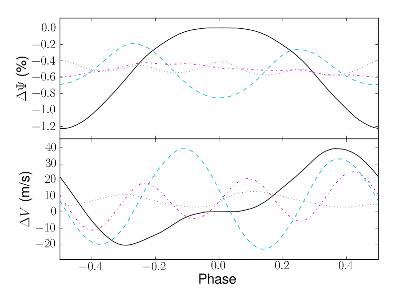
Figure 3: Photometric and RV signatures of spot distributions matching low-order multipoles with 1, 2, 3 and 4 nodes along the equator (solid black, dashed cyan, dash-dot magenta and dotted grey line respectively). The spot distributions are uniform in $\sin(\delta)$. The stellar parameters are identical to the fiducial values used in Figure 1.

The $FF^{\prime}$ method rests on the assumption that the photometric signal contains sufficient information to adequately predict the RV signal. We test this assumption here by examining the relative amplitudes and shapes of photometric and RV signals from spot distributions approximating low-order multipoles in the longitudinal direction. We simulated light and RV curves for stars with 200 spots, each with $c=0$ and $\alpha=0.01^{\circ}$. The spot longitudes $\phi_{0}$ were drawn at random from the desired distribution, and their latitudes were taken from a uniform distribution in $\sin(\delta)$. All the parameters of each spot were fixed (no spot evolution) and all spots shared the same rotation rate (no differential rotation).

The results of these tests are shown in Figure 3. While both photometric and RV signals are sensitive to dipole (black line) and quadrupole (dashed cyan line) configurations, the photometric signal is only very marginally sensitive to higher order odd-numbered multipoles (e.g. order $3$, dash-dot magenta line), which do give rise to some RV variation. This can be understood intuitively as a consequence of the symmetry of the problem. The same phenomenon has already been noted by Cowan & Agol (2008) in the context of phase-function mapping of exoplanets: sinusoidal maps with odd order have no photometric phase function signature. Conversely, the RVs are not very sensitive to higher order even-numbered multipoles (e.g. order $4$, dotted grey line) configurations, although this is less noticeable. This implies that any attempt to simulate activity-induced RV variations based on photometry – whatever the method – is likely to over-estimate the signal at high-$n$ (even-numbered) harmonics, and underestimate that at high-$m$ (odd-numbered) harmonics.

4.2 Simulations using multiple, evolving active regions

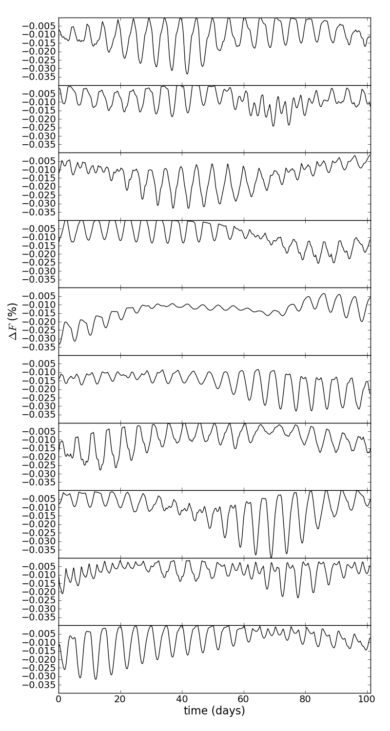
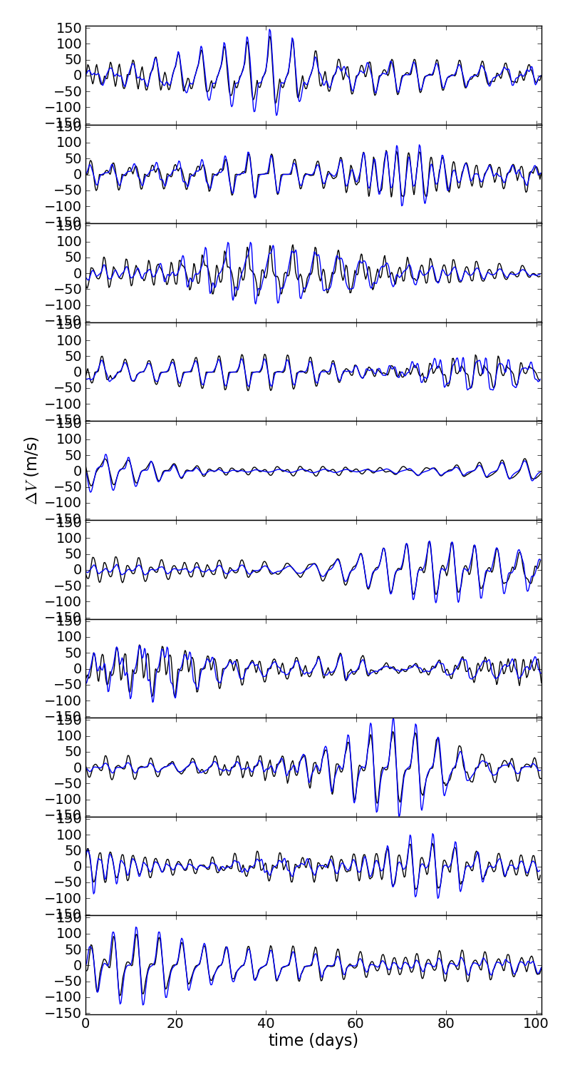
Figure 4: Simulation examples: flux variations simulated with the spot model (left), RV variations (middle) produced by the spot model (blue) and by the $FF^{\prime}$ method applied to the flux data shown in the left panel (black), and corresponding periodograms (right). These 10 examples were selected at random from the 100 simulations with 20 spots.

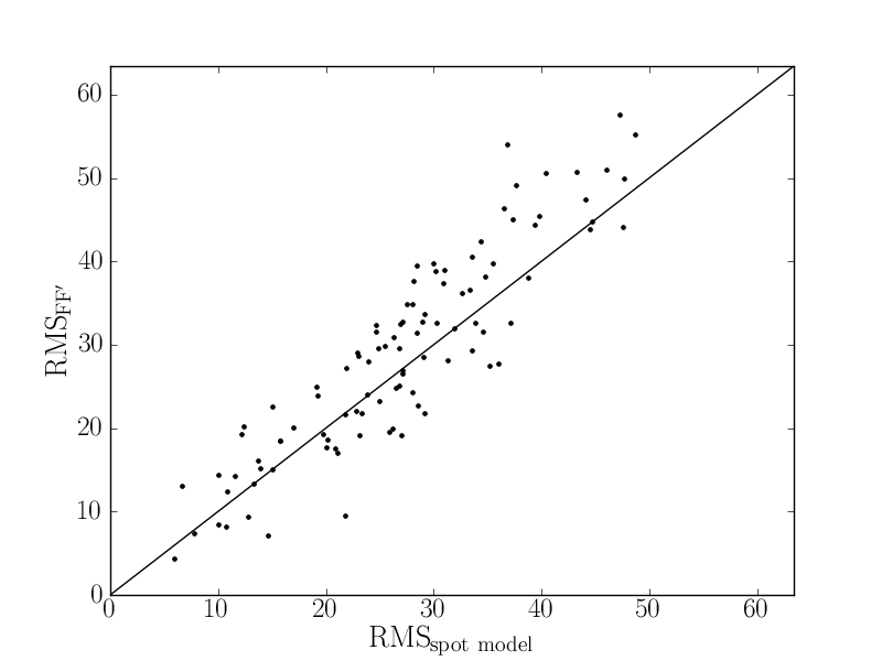
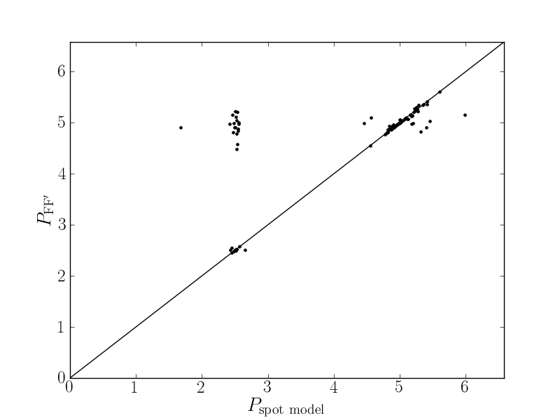
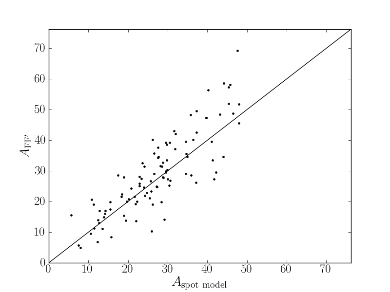
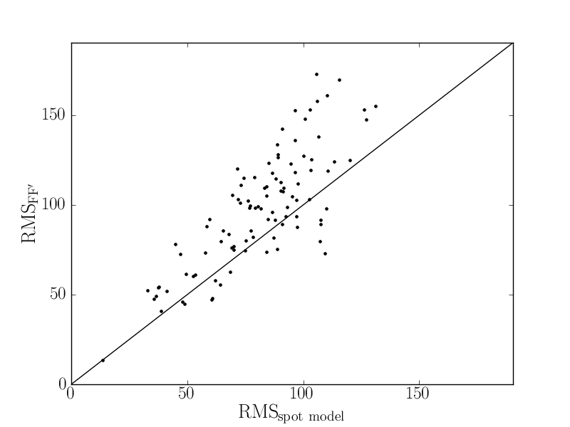
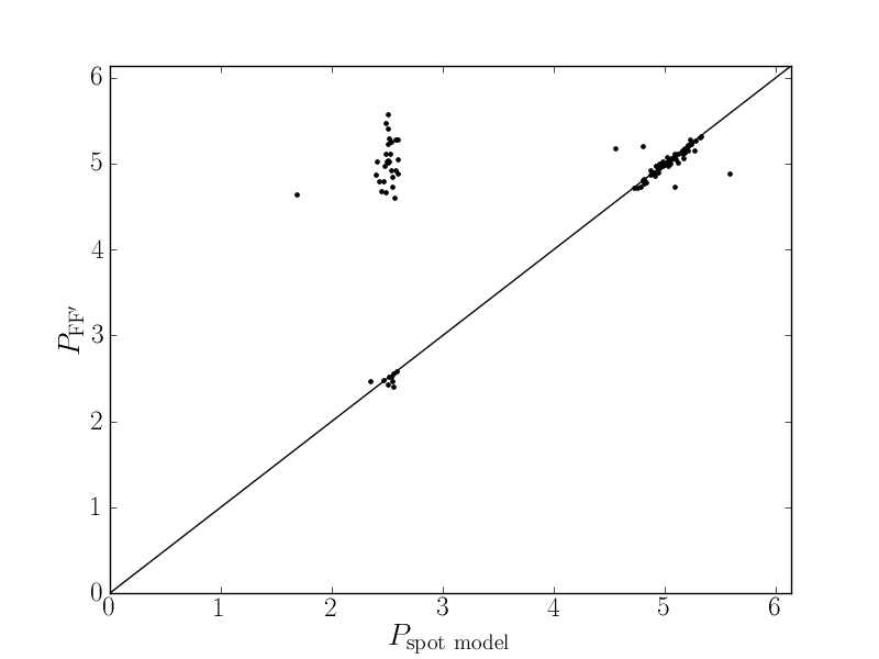
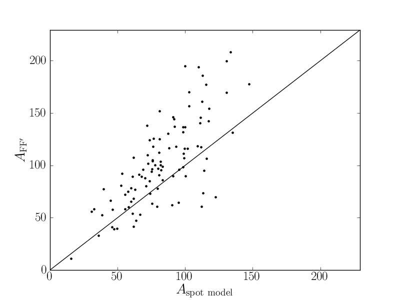
Figure 5: Comparison of RV variations simulated with our spot model (x-axis) to the predictions of the $FF^{\prime}$ method applied to the photometric output of the same simulations (y-axis). The left, middle and right column show the time-series RMS scatter, the period and the amplitude of the best-fitting sinusoidal modulation, while the top and bottom rows correspond to 20 and 200 spots, respectively. The black line in each panel follows $y=x$.

We used the spot model described in Section 2 to generate flux, RV and bisector span time series and test the ability of the $FF^{\prime}$ method to recover the RV signal based on the flux information only.

We generated 100 time-series lasting 100 days each, each with 20 randomly distributed, evolving, differentially rotating spots, and another set of 100 time-series with 200 spots. We computed photometric and RV time-series lasting 100 days, with one point every 0.05 day. For each realisation, the stellar inclination was drawn at random from a distribution uniform in $\cos(i)$, and the spots were distributed uniformly in $\sin(\delta)$, and rotated differentially depending on their latitude, following $P(\delta)=P_{0}+0.1\sin(\delta)$, with $P_{0}=5$ days in all cases. The angular size $\alpha$ of each spot followed a squared exponential growth and decay, with $e$-folding times drawn from a log-normal distribution with mean $0.4\log P_{0}$ and standard deviation 0.15. The peak times were drawn from a uniform distribution over the range $[-L/2,3L/2]$, where $L$ was the light curve duration.

The purpose of these simulations is to identify fundamental limitations of the method, rather than to evaluate its performance in fully realistic conditions. Therefore, we did not add noise to the simulated data. Each photometric time-series was processed with the $FF^{\prime}$ method, as outlined in Section 3.2, to generate synthetic RVs. As no noise was added, no smoothing was necessary. The resulting RVs are compared to the output of the spot model for a subset of the simulations in Figure 4. There is generally very good agreement between the time series, but the $FF^{\prime}$ RVs occasionally depart from the output of the spot model by up to a third of the peak-to-peak amplitude. In those cases, the periodograms (which otherwise show excellent agreement) show a different ratio between the odd- and even-numbered harmonics. This occurs when the spot distributions approximate odd-numbered multipoles: as noted in the previous section, this causes RV variations with virtually no counterpart in photometry. In other words, as expected, RV variations at the fundamental and first harmonic are well reproduced by the $FF^{\prime}$ output and strongly suppressed in the residuals (often by as much as 80%), but variations at higher, even-numbered harmonics remain, and can even be enhanced.

We also computed and compared the overall RMS of the ‘true’ (spot-model) RVs, the $FF^{\prime}$output, and the residuals, and the best fit sinusoidal period and amplitude in the $FF^{\prime}$ output compared to the true RVs. The RMS of the residuals is reduced by $>50\%$ compared to the original value in 54% of the simulations with 20 spots, but this performance is achieved in only 16% of the simulations with 200 spots. This is because, when there are so many spots, the spot distribution almost always has an odd-numbered multipole component. Nonetheless, as shown in Figure 5, the RMS, amplitude and period of $FF^{\prime}$ output are always well-correlated with the corresponding values for the ‘true’ RVs. For simulations using 20 spots, the Pearson correlation coefficients for the RMS and amplitudes are 0.90 and 0.84, respectively, with slightly lower values of 0.80 and 0.75 for 200 spots. There is a slight tendency for the $FF^{\prime}$ to over-predict the amplitude of the variations: linear fits to the scatter plots shown in Figure 5 yield slopes of 1.08 and 1.06 (1.1 and 1.17) for the RMS and amplitude respectively, for 20 (200) spots. The period, or its first harmonic, is almost always correctly recovered (up to a precision of 10%). Incidentally, the fraction of the cases where the first harmonic dominates over the fundamental is smaller for the $FF^{\prime}$ output than for the direct spot-model simulations.

Thus, except in particularly favourable cases, the $FF^{\prime}$ method does not enable a precise ‘correction’ of the RV variations due to activity, prior to searching for low mass planets, for example. However, it does permit a statistical comparison in terms of amplitudes and frequency content. Nonetheless, further tests on real data are desirable to establish the performance of the $FF^{\prime}$ method on a firmer footing.

4.3 Application to HD 189733

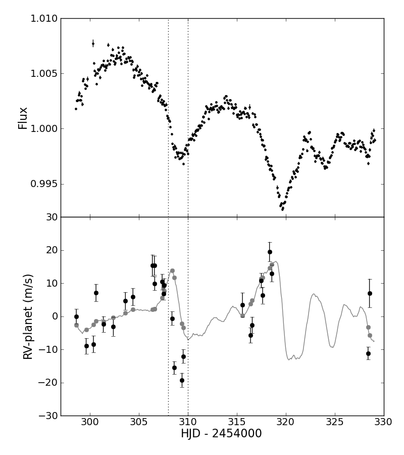
Figure 6: Photometry and RV time-series for HD 189733. The MOST light curve (Boisse et al., 2009) is shown in the top panel and the observed and simulated RV data are compared in the bottom panel. The black dots with error bars show the SOPHIE data from Lanza et al. (2011) after removal of the best-fit planetary signal, and subtraction of a constant 21.6 m s^-1 offset. The grey line shows the RV curve simulated by applying the $FF^{\prime}$ method to the MOST light curve, and the grey dots show the same curve linearly interpolated to the sampling of the SOPHIE observations.

The transiting planet host star HD 189733 was the target of intensive simultaneous monitoring with the RV spectrograph SOPHIE and the photometric satellite MOST. An in-depth analysis of these observations from the activity point-of-view was already presented in Boisse et al. (2009). This dataset constitutes a useful test for RV jitter simulation methods based on photometry, and was recently used for this specific purpose by Lanza et al. (2011).

Starting from the MOST light curve, which is shown in the top panel of Figure 6, we simulated the expected activity-induced RV variations using the $FF^{\prime}$ method. The light curve was first smoothed using the iterative non-linear filter of Aigrain & Irwin (2004) using a baseline of 6 data points ($\sim 10$ h) to reduce the noise on the time-derivative estimate. The results are shown as the grey line in the bottom panel of Figure 6. We then compared this to the SOPHIE observations, which are shown as black dots. Note that we used the new reduction of the SOPHIE data, as described by Lanza et al. (2011), and worked with the residuals of the planetary orbit (I. Boisse, priv. comm.). Following Lanza et al. (2011), we subtracted a constant offset of 21.6 m s^-1 from the SOPHIE orbit residuals. We then linearly interpolated the $FF^{\prime}$ output to the sampling of the SOPHIE observations (grey dots in Figure 6).

The interpolated $FF^{\prime}$ output is a good match to the orbit residuals except from ${\rm HJD}=2\,454\,308$ to $2\,454\,310$, and is virtually identical to the Lanza et al. (2011) results throughout. The latter already noted that their model could not reproduce the very rapid drop observed in the RVs around this time. One possible explanation may be that the spot distribution around this time had a significant odd-numbered multipole component, which no photometry-based method could recover. However, we note that, around ${\rm HJD}=2\,454\,308$, the observed flux also dips faster than can be reproduced by an unevolving surface feature rotating into view. This suggests that there are rapidly evolving active regions on the star at this time, a situation which neither the $FF^{\prime}$ method nor the method of Lanza et al. (2011) are well suited for.

The reduced $\chi^{2}$ of the SOPHIE orbit residuals (excluding the problematic interval from ${\rm HJD}=2\,454\,308$ to $2\,454\,310$) is 14.45, and their r.m.s is 9.4 m s^-1. Subtracting the activity contribution, as predicted by the $FF^{\prime}$ method, reduces the reduced $\chi^{2}$ by a factor $>2$ to 6.58, and the r.m.s to 6.6 m s^-1. Although the presence of a residual activity signal cannot be excluded, the final r.m.s is consistent with the level of instrumental systematics typical of SOPHIE at the time of the HD 189733 observations ($\sim 5$ m s^-1, Boisse priv. comm.).

We also computed the Lomb-Scargle periodogram of the RV data before and after subtracting the simulated activity signal (Figure 7). For this calculation, we used only data simultaneous with the MOST observations, and excluded the aforementioned discrepant data points. Again the results are almost identical to Figure 6 of Lanza et al. (2011). Subtracting the output of the $FF^{\prime}$ method suppresses power at the rotational frequency by a factor close to 10, and gradually decreasing fractions of the power at each harmonic. The last significant peak (the third harmonic) is suppressed by a factor of $\sim 2$ only.

In summary, despite its simplicity, the $FF^{\prime}$ method gives results that, at least in this specific case, are equivalent to the more sophisticated approach of Lanza et al. (2011), and achieves the same performance in terms of RV power suppression. One possible explanation for this is that the maximum entropy regularisation employed by Lanza et al. (2011) effectively places a prior on the spatial and temporal scales accessible to their model. This has a similar effect to the approximations made in the $FF^{\prime}$ method, which is only a first order approximation to the full expression for multiple spots, and is therefore expected to match the signature of the dominant active regions only. Therefore, one should be cautious not to over-interpret the output of both models, particularly as regards short-term behaviour – unfortunately, a detailed comparison of the two methods in the short-timescale regime is difficult because the RV data for HD 189733 have relatively sparse time-sampling, and uncertainties comparable to the short-term activity signal.

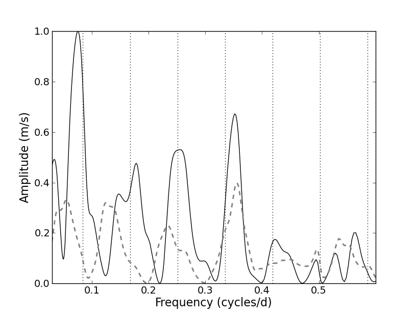
Figure 7: Lomb-Scargle periodograms of the observed RV time-series for HD 189733 after subtracting only the planetary orbit (solid black line) and after removing the simulated activity signal also (dashed grey line). Both RV datasets have the same time sampling, including only SOPHIE data points simultaneous with the MOST observations, and excluding the 4 data points between the vertical dashed lines in Figure 6. The rotational frequency and its harmonics are indicated by the vertical dotted lines. Following Boisse et al. (2009), we took the rotation period to be 11.953 days.

4.4 The Sun

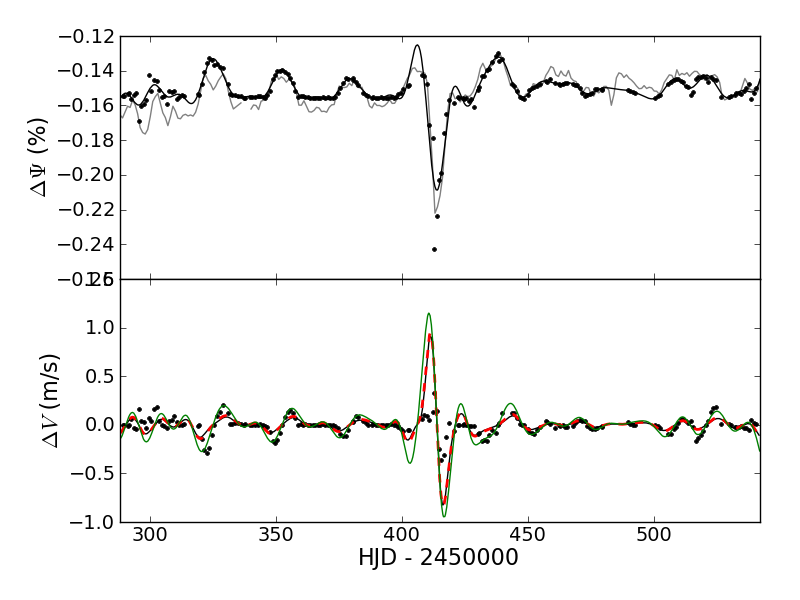
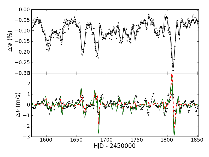
Figure 8: Application of the $FF^{\prime}$ to synthetic solar data. The black dots show the synthetic TSI (top panel) and RV (bottom panel) variations of the Sun, from Meunier et al. (2010b), for two 6-month periods when the Sun was relatvely inactive (left) and active (right). In each case, the solid black line in the top panel shows the smoothed version of the synthetic TSI used as input to the $FF^{\prime}$. The measured TSI (SoHO/VIRGO daily average, from http://www.pmodwrc.ch/, maintained by C. Fröhlich) is also shown for comparison as the solid grey line. The solid black, thick dashed red and solid green lines in the bottom panel then show the $FF^{\prime}$ predictions based on that smoothed TSI, using different values of $\Psi_{0}$ and $\kappa\delta V_{\rm c}$ (see text for details).

The Sun, as the nearest and best-studied star available to us, is an ideal test case for the $FF^{\prime}$ method. Its brightness and RV variations have been intensively monitored for decades, from space (e.g. by the SoHO satellite) and from the ground (e.g. by the GONG and BiSON networks). However, solar RV monitoring projects are primarily intended to study the Sun’s 5-minute oscillations, and we were not able to find a publicly available set of full-disk RV measurements that were calibrated over long timescales.

We therefore used the synthetic dataset of Meunier et al. (2010b). This dataset was generated by identifying different types of magnetic features on SoHO/MDI magnetograms, and simulating their effect in both photometry and RV, tuning the model to fit the total solar irradiance (TSI) variations observed by SoHO/VIRGO. We focus on two 6-month long sections at opposite phases in the solar cycle, one during a period of relatively low activity, and one during a period of relatively high activity. For each, we were provided with synthetic TSI and RVs sampled approximately once per day (A.-M. Lagrange, priv. comm.). The synthetic RVs are, of course, subject to the limitations of the Meunier et al. (2010b) model. However, applying the $FF^{\prime}$ to the synthetic TSI, and comparing the results to the synthetic RVs at least provides an internal consistency check. In particular, it is a fairly stringent test of the very limited treatment of faculae and plage used in the $FF^{\prime}$ method, since the latter are the dominant effect in the synthetic RVs.

As can be seen in the top panel of Figure 8, the synthetic TSI (black dots) is a good match to the observed TSI (grey line), but it is not smooth. Its time-sampling is also slightly irregular and relatively sparse ($<1$ point per day). This makes smoothing using the iterative non-linear filter discussed in Section 3.2, which gave satisfactory results for the MOST time-series of HD 189733 in Section 4.3, inappropriate for this dataset. Instead, we performed a Gaussian process (GP) regression on the synthetic TSI. More details on the GP regression are given in Appendix B.

The resulting smoothed TSI (shown as the black solid line in the top panel of Figure 8) was then fed in to the $FF^{\prime}$ method, and the results are compared to the synthetic RVs in the bottom panel. We first used Equation (13) to estimate $\Psi_{0}$, and set $\kappa\delta V_{\rm c}$ to zero (black line). We also tried fitting for those two parameters, using a downhill simplex optimizer to minimize the sum of the squared differences between the synthetic RVs and the $FF^{\prime}$ output linearly interpolated to the same time-sampling (thick red dashed line). Finally, we also tried setting $\Psi_{0}$ to 1, corresponding to an absolute irradiance of $1367.62\,{\rm W}/{\rm m}^{2}$, which is approximately the maximum irradiance observed at any time during the last solar activity cycle (green line, $\kappa V_{\rm c}$ was again set to zero). In the low-activity case, the red and black lines are identical, with best-fit parameters $\Psi_{0}=0.99887$ and $\kappa\delta V_{\rm c}=12.7$ m s^-1. The three versions have very similar r.m.s. residuals, this time $\sim 0.06$ m s^-1. In the high-activity case, it is the green and black lines (and the corresponding values of $\Psi_{0}$) which are virtually indistinguishable, whereas the best-fit parameters used to produce the red curve are $\Psi_{0}=0.99926$ and $\kappa\delta V_{\rm c}=417$ m s^-1. Again, the three versions have very similar root mean square (r.m.s.) residuals, $\sim 0.5$ m s^-1. In both the low- and high-activity cases, fixing $\Psi_{0}$ to 1 appears to give a better match visually than fitting for it, but it yields a slightly larger squared error and residual r.m.s.

The most significant deviations between the synthetic and $FF^{\prime}$ RVs occur when a large sunspot group causes a sudden drop in the TSI, e.g. near ${\rm HJD}-2450413$. This necessarily induces a similarly large variation in the $FF^{\prime}$ output, which has no counterpart in the synthetic RVs of Meunier et al. (2010b). There are several possible reasons for these discrepancies: the insensitivity of the photometry to certain spot configurations, the limited treatment of faculae and plage in the $FF^{\prime}$ method, or unidentified issues with the synthetic RVs themselves. In the absence of measured solar RVs to provide a ground truth, all these possibilities must remain open.

Nonetheless, the overall agreement between the $FF^{\prime}$ output and the synthetic RVs is very encouraging. This implies that the $FF^{\prime}$ method can certainly be used to study RV variations down to the m s^-1 level.

4.5 Application to Kepler data

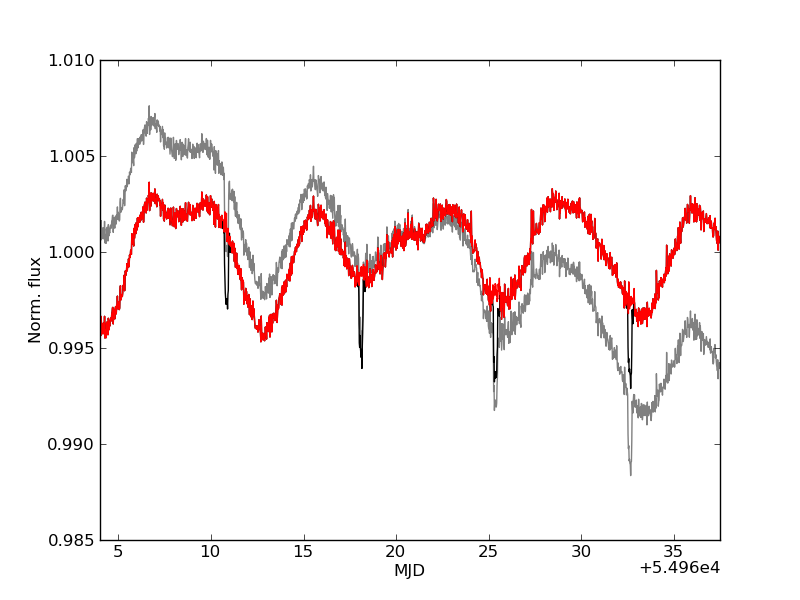
Figure 9: Example Kepler Quarter 1 light curve before and after applying our systematics correction. The original, raw time-series is shown in grey, the corrected time-series in black, and the corrected time-series without the transits (used to estimate the RV modulations) in red. Note that the red line completely overlaps with the black, except during the transits. This example is KID 3642741 (KOI 242).

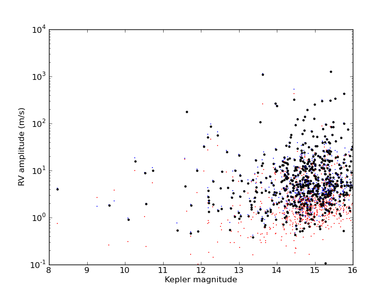
Figure 10: Application of the $FF^{\prime}$ to Kepler quarter 1 light curves containing planet candidates. The small blue dots show the RV amplitudes derived from the light curves after removing the transits and smoothing on one tenth of the dominant light curve period, while the small red dots show the RV amplitude expected for a white noise-only light curve with the same high-frequency noise level, smoothed to the same extent. The black dots show the noise-corrected RV amplitude estimates, obtaining by subtracting the latter from the former in quadrature.

Given a sample of high-precision, high time-sampling light curves, the $FF^{\prime}$ method can be used to estimate the statistics of the activity-induced RV variability of the same sample of stars. The tens of thousands of high-precision light curves produced by the Kepler mission constitute an ideal dataset to do this. A systematic application of the $FF^{\prime}$ method to individual Kepler light curves is beyond the scope of this paper, but as an illustration we now proceed to apply it to a subset of the light curves in which the Kepler team identified transiting planet candidates (Borucki et al., 2011).

The Kepler photometric pipeline produces two versions of the light curves: a ‘raw’ time-series, and a version corrected for most of the systematic instrumental effects. In the current version of the pipeline, this correction unfortunately also removes much of the intrinsic variability of the target stars. In the context of a separate study, focussed on the statistics of photometric variability in Kepler data, we have developed a more conservative systematics removal correction, which is designed to preserve astrophysical signals. This correction will be described in detail in a forthcoming paper, so we only summarise the underlying principles here. Each light curve is decomposed into a linear combination of all the other light curves, plus an intrinsic component, using Bayesian linear regression. The most significant trends that are common to many light curves are identified using an information entropy criterion. They are then combined using principal component analysis, de-composed into their intrinsic oscillatory modes, and removed from each individual light curve, again using Bayesian linear regression. The process is repeated iteratively until no further trends are identified. The correction is currently available only for the data from Quarter 1, which were released to the public on June 15, 2010. We therefore focus on 601 of the 997 stars with planet candidates announced by Borucki et al. (2011), whose light curves were included in that release, and treat only the Quarter 1 data, which lasts 33 days. An example of the systematics correction applied to one of these objects is shown in Figure 9.

After masking the transits, we first computed the periodogram of each light curve to identify the dominant periodicity, restricting the search to the range $0.5$–$50$ days. The periods were not checked individually, and there is no guarantee that they are related to a real, physical period (such as the rotation period of the target star). However, we use them to smooth the light curves, by applying the iterative non-linear filter of Aigrain & Irwin (2004), with a smoothing time-scale equal to one tenth of the identified period. We then apply the $FF^{\prime}$ method to the smoothed light curve. The results are, of course, affected not only by the intrinsic variability of the host star, but also by any photometric noise still present in the smoothed light curve. The latter depends not only on the stars’ magnitude, but also on the smoothing timescale used, which varies from star to star. This is unavoidable – excessive smoothing of a light curve with real, short-term variability would lead to under-estimated RV variations – but it is important to quantify the residual noise contribution to the RVs. In each case, we therefore also computed the RV variations expected for a simulated light curve containing only white Gaussian noise at the same level as the original, smoothed using the same timescale. The noise level was estimated as the standard deviation of the original light curve minus the smoothed version thereof. The noise-only RV amplitude was subtracted from the amplitude derived from the real light curve, yielding an estimate corrected for photometric noise.

Figure 10 shows the resulting RV peak-to-peak amplitudes over the duration of Quarter 1, as a function of Kepler magnitude. The small blue dots show the amplitude measured for the real light curves, and the small red dots the corresponding amplitudes for noise-only light curves, and the black dots show the noise-corrected estimates. The distribution of the red points shows that the Kepler light curves can be used to estimate RV variations down to the 2–3 m s^-1 level, below which they become noise-dominated in most cases. The distribution of the noise-corrected amplitudes is approximately log-normal, with a mean of $\sim 4.1$ m s^-1 and a width of $\sim 0.45$ dex. Approximately two thirds of the candidates are expected to display RV variations significantly above the noise limit. This does not translate directly into implications for the detectability of the RV signatures of the transit candidates, as the intrinsic RV variations may occur on timescales which are quite distinct from the orbital period. Nonetheless, it does suggest that RV confirmation would be challenging for these candidates, the majority of which have radii below that of Neptune (for comparison, the expected RV-semi-amplitude for a Neptune-mass planet in a 10 day orbit around a Sun-like star is $\sim 5$ m s^-1). The predicted amplitude of the activity-induced RV signal is below the noise level for the remaning third of the candidates.

5 Conclusions

We have presented a new method to derive the stellar variability expected in RV measurements from well-sampled light curves, which requires no knowledge of the rotation period or detailed spot modelling. We call this method $FF^{\prime}$ because it uses the light curve and its first derivative. A number of approximations are built into our method: in particular, it ignores limb-darkening, as well as the photometric effect of faculae (but not their RV signature), and the expression used to compute the RV signal is accurate only to first order when multiple spots are present on the stellar surface. However, the observables (photometry and RV) are disk-integrated quantities, which mitigates the impact of these approximations.

We tested this $FF^{\prime}$ method on time-series simulated using the simple spot model on which it is loosely based. Overall, our simulations show that the RMS, period and amplitude of periodic modulation of $FF^{\prime}$ predictions are in fairly good agreement with the corresponding model values. Given its simplicity, our method reproduces activity-induced variability surprisingly well, matching the latter’s amplitude and distribution of power at the first few harmonics of the rotational frequency to $\sim 10\%$ or better in most cases. There are exceptions, where the power at odd-numbered harmonics is not well-matched. To understand this phenomenon, we used our spot-model to explore the relationship between photometric and RV variations due to spots in the general sense, and showed that any method which uses photometry to simulate RVs will struggle to reproduce the signals if spot distribution has a significant odd-numbered multipole component.

We then applied the $FF^{\prime}$ method to three example datasets: the benchmark SOPHIE/MOST observations of HD 189733, synthetic TSI and RV data for the Sun, and the Quarter 1 light curves of Kepler planet candidate host stars.

For HD 189733, our results are essentially identical to those obtained by Lanza et al. (2011) with a much more sophisticated method, reducing the power of the RV variations at the rotational frequency by a factor $\sim 10$, and by a factor of a few at the first few harmonics. Where both approaches struggle to reproduce some of the observed RV variations, we identify a possible explanation in their common reliance on the photometry to predict the RVs.

The solar tests demonstrate the performance of the method down to the sub-m s^-1 level. We show that, given enough high-quality RV data, it is possible to fit for the un-spotted flux level, but this has only a relatively minor impact, and the results obtained by estimating it from the light curve itself are almost as good. We also show that it is possible to fit for the parameter $\kappa\delta V_{\rm c}$, which controls the importance of the convective term, but again this has relatively little effect on the results. These tests also illustrate the use of Gaussian processes, rather than simpler filters, to interpolate and smooth the photometric time-series. This opens up the possibility of applying the $FF^{\prime}$ method to cases where there is only sparse photometry, or where a photometric proxy is derived from the same spectra as the RV observations themselves.

Finally, we have shown that the $FF^{\prime}$ method can be used to estimate RV amplitudes down to the 2–3 m s^-1 level using Kepler data. Approximately two thirds of the 600 planet candidate host stars to which we applied it are expected to display peak-to-peak RV amplitudes over 30-day timescales that are above that level. This confirms that obtaining mass measurements for many of the Kepler terrestrial and/or longer-period planet candidates will be challenging. However, it also opens up a range of possibilities for identifying the most promising candidates to follow up, and perhaps disentangling activity- and planet-induced RV signals for those objects. We caution that, like all methods based on photometry, some care must be taken when interpreting the output of the $FF^{\prime}$ method for individual objects. Nonetheless, we have shown that it performs as well in that respect as other methods which have already been put to that use.

The distinguishing characteristic of the $FF^{\prime}$ method, however, is its simplicity, speed, and lack of free parameters. In its simplest implementation, all it requires is an estimate of the stellar radius. The method can thus be applied to large samples of light curves such as those produced by the CoRoT and Kepler missions, to assess the RV jitter properties of a large sample of stars, and their implications for the detection of habitable planets by RV. No other method we are aware of can be applied to a large enough sample of light curves to undertake such a project, which would form a natural extension to the present paper.

Appendix A Calculations underlying the spot model

A.1 Trajectory of the spot

Consider a spot located at latitude $\delta$ on the surface of a star with radius $R_{\star}$ rotating with period $P_{\rm rot}$ and inclination $i$ (where $i$ is defined as the angle between the star’s rotation axis and the line-of-sight). We define two reference frames $S$ and $S^{\prime}$, sharing the same origin, which coincides with the centre of the star, and the same $y$-axis. The stellar rotation vector defines the $+z$-direction of frame $S$, whilst the $x$-axis of frame $S^{\prime}$ points towards the observer. In frame $S$, the location of the spot is given by:

$$\frac{1}{R_{\star}}\left[\begin{array}[]{l}x\\ y\\ z\end{array}\right]=\left[\begin{array}[]{l}\cos\delta\cos\phi\\ \cos\delta\sin\phi\\ \sin\delta\end{array}\right],$$

where $\phi=2\pi t/P_{\rm rot}+\phi_{0}$ and $\phi_{0}$ is the longitude of the spot at $t=0$. The coordinates of the spot in frame $S^{\prime}$ are then obtained by performing a rotation by angle $-(\pi/2-i)$ about the $y$ axis:

$$\begin{array}[]{rcl}\frac{1}{R_{\star}}\left[\begin{array}[]{l}x^{\prime}\\ y^{\prime}\\ z^{\prime}\end{array}\right]&=&\left[\begin{array}[]{lll}\sin i&0&+\cos i\\ 0&1&0\\ -\cos i&0&\sin i\\ \end{array}\right]\left[\begin{array}[]{l}\cos\delta\cos\phi(t)\\ \cos\delta\sin\phi(t)\\ \sin\delta\end{array}\right]\\ &=&\left[\begin{array}[]{l}\cos\delta\cos\phi(t)\sin i\ +\sin\delta\cos i\\ \cos\delta\sin\phi(t)\\ -\cos\delta\cos\phi(t)\cos i+\sin\delta\sin i\end{array}\right].\end{array}$$

A.2 Relative drop in flux due to the spot

To calculate the quantities of interest, we need to evaluate $\beta$, the angle between the spot normal and the line of sight. It is easy to show (for example using the cosine rule on the triangle defined by the spot’s position vector and its projection onto the line-of-sight) that this angle is simply given by

$$\cos\beta=x^{\prime}/R_{\star}=\cos\delta\cos\phi(t)\sin i+\sin\delta\cos i.$$

The relative drop in observed flux $F$, described by equation (1), follows the same time dependence.

In frame $S$, the vector describing the rotational motion of the stellar surface at the location of the spot is given by

$$V_{\rm rot}=\left[\begin{array}[]{l}-V_{\rm eq}\cos\delta\sin\phi\\ V_{\rm eq}\cos\delta\cos\phi\\ 0\end{array}\right]$$

where $V_{\rm eq}=2\pi R_{\star}/P_{\rm rot}$. In frame $S^{\prime}$ this becomes

$$\begin{array}[]{rcl}V^{\prime}_{\rm rot}&=&\left[\begin{array}[]{lll}\sin i&0&-\cos i\\ 0&1&0\\ \cos i&0&\sin i\\ \end{array}\right]\left[\begin{array}[]{l}-V_{\rm eq}\cos\delta\sin\phi\\ V_{\rm eq}\cos\delta\cos\phi\\ 0\end{array}\right]\\ &=&\left[\begin{array}[]{l}-V_{\rm eq}\cos\delta\sin\phi\sin i\\ V_{\rm eq}\cos\delta\cos\phi\\ V_{\rm eq}\cos\delta\sin\phi\cos i\\ \end{array}\right].\end{array}$$

The time dependence of the RV signature of the spot, $\delta RV_{\rm s}$, is governed by the $x$-component of this vector times $F(t)$.

The net convective up-welling velocity is radial, so its line-of-sight component is simply:

$$\delta V^{\prime}_{\rm c}=\delta V_{\rm c}\cos\beta.$$

Appendix B Gaussian process regression on the total solar irradiance

In order to apply the $FF^{\prime}$ method to the solar data, we need to convert the irregularly sampled, discontinuous synthetic TSI to a smooth, tightly sampled flux estimate. We do this using Gaussian process (GP) regression.

GP models are extensively used in the machine learning community for Bayesian inference in non-parametric regression and classification problems. By definition, any vector of observations drawn from a Gaussian process has a joint distribution which is a multi-variate Gaussian. Families of random functions which share the same smoothness and covariance properties can be parametrised in terms of a covariance function or kernel, which specifies the covariance between pairs of points as a function of – typically – the distance between these points in some input space (e.g. the time interval between two observations). Thus, GP regression is particularly well-suited to modeling time-series containing correlated stochastic signals and noise. A brief introduction to GP regression, with an application to space-based, high-precision stellar photometry, albeit in a different context (exoplanet transmission spectroscopy), can be found in Gibson et al. (2011). The textbook by Rassmussen & Williams (2006) provides a more detailed treatment of GPs for both regression and classification.

The most important step in GP regression is the choice of covariance function, or kernel. Most kernels are decreasing functions of the distance between pairs of points in the input space. One of the simplest and most widely used kernels is the squared exponential:

$$k_{\rm SE}(t,t^{\prime})=\theta^{2}\exp\left(-\frac{r}{2\tau^{2}}\right).$$ (15)

where $k_{\rm SE}(t,t^{\prime})$ is the covariance between observations taken at times $t$ and $t^{\prime}$, and $r\equiv|t-t^{\prime}|$ is the time interval between the two observations, $\theta$ is a parameter controling the amplitude of the flux variations, and $\tau$ is a parameter controlling the time-scale of the flux variations.

Visual examination of the synthetic solar TSI indicated that the data might contain variations on more than one time-scale. Such behaviour can be modelled using a rational quadratic kernel:

$$k_{\rm RQ}(t,t^{\prime})=\theta^{2}\left(1+\frac{r}{\alpha l^{2}}\right)^{-\alpha}$$ (16)

where $\alpha$ is an additional parameter, controling the distribution of timescales. Indeed, it can be shown (Rassmussen & Williams, 2006) that the rational quadratic kernel is equivalent to a superposition of an infinite number of squared exponential kernels with a distribution of time-scales $\tau$ that is a power-law of index $-\alpha$. When $\alpha\rightarrow\infty$, the rational quadratic kernel approximates the squared exponential kernel. For finite $\alpha$, the rational quadratic implies significantly more covariance at relatively large separation than the squared exponential (equivalent to a ‘long tail’ behaviour).

Stellar light curves, which display the effects of rotationally modulated, evolving active regions, tend to be quasi-periodic. This kind of behaviour can also be modelled by a GP, using a periodic kernel multiplied by a squared exponential term:

$$k_{\rm QP}=\theta^{2}\exp\left(-\frac{\sin^{2}(\pi r/P)}{2T^{2}}-\frac{r}{2\tau^{2}}\right).$$ (17)

where $P$ is the period in days, $T$ is the time-scale of variations within a period, and $\tau$ is now the evolution time-scale (also in days), controling the rate of change of the shape and amplitude of the signal from one period to the next. We could also have combined the periodic term with a rational quadratic term, but initial experiments with that possibility indicated that this gave too much freedom to the model.

These are only some of the possible kernels which are relevant to the type of dataset we are trying to model here, see Rassmussen & Williams (2006) for a more detailed discussion of covariance functions. For a given set of kernel parameters, the GP defines a probability distribution over functions sharing the same covariance properties. This distribution can be conditioned on any available observations, yielding a predictive distribution which can be used to interpolate the data to the desired sampling. The process also yields a marginal likelihood, which can be maximised with respect to the kernel parameters (which are also known as the hyper-parameters of the GP) in order to optimise the latter.

We experimented with all the kernels listed above on the synthetic solar TSI, adding a delta-function to represent white noise:

$$k_{\rm tot}(t,t^{\prime})=k(t,t^{\prime})+\theta_{\rm w}\delta(r).$$ (18)

In fact, the synthetic data we are modeling contain no explicit white noise term, but the addition of a small constant noise term to the diagonal elements of the covariance matrix significantly helps convergence.

In the high-activity case, the squared exponential kernel yielded a poor fit to the data (low marginal likelihood after optimising the hyper-parameters): a single time-scale is not sufficient to model the data. The quasi-periodic kernel also gave a relatively low marginal likelihood, with a short period (unrelated to the known solar rotation period), $T\gg 1$ and $\tau\ll P$ (note that, unlike $\tau$, $T$ is dimensionless, because it divides the $\sin^{2}$ term, which varies between 0 and 1). This implies that the active regions are evolving on timescales comparable to, or shorter than, the rotation period. With such a combination of hyper-parameters, the quasi periodic GP behaves essentially like the squared exponential. The best results were obtained with the rational quadratic kernel, with $\theta=0.0004$, $\alpha=1.5$, $\tau=2.9$ days and $\theta_{\rm w}=0.0001$ respectively ($\theta$ and $\theta_{\rm w}$ are in units of relative flux and $\alpha$ is dimensionless). The mean of the predictive distribution obtained with these hyper-parameters was used as the smoothed TSI.

In the low-activity case, the best results were obtained with the squared exponential kernel, with $\theta=0.001$, $\tau=12.7$ days and $\theta_{\rm w}=0.00005$. When using the rational quadratic kernel, the best-fit value of $\alpha$ was very large – which approximates the behaviour of a squared exponential kernel. When excluding the sunspot crossing around ${\rm HJD}=2450413$, the quasi periodic kernel gave relatively good results with best-fit hyper parameters $\theta=0.0008$, $P=28.9$, $T=1.4$, $\tau=48.3$ and $\theta_{\rm w}=0.00002$. However, this kernel could not reproduce the TSI during the aforementioned sunspot crossing, so we used the squared exponential to generated the smoothed TSI.

References

- Aigrain & Irwin (2004) Aigrain S., Irwin M., 2004, MNRAS, 350, 331
- Boisse et al. (2011) Boisse I., Bouchy F., Hébrard G., Bonfils X., Santos N., Vauclair S., 2011, A&A, 528, 4
- Boisse et al. (2009) Boisse I., Moutou C., Vidal-Madjar A., Bouchy F., Pont F., Hébrard G., Bonfils X., Croll B., Delfosse X., Desort M., Forveille T., Lagrange A.-M., et al. 2009, A&A, 495, 959
- Bonfils et al. (2007) Bonfils X., Mayor M., Delfosse X., Forveille T., Gillon M., Perrier C., Udry S., Bouchy F., Lovis C., Pepe F., Queloz D., Santos N. C., Bertaux J.-L., 2007, A&A, 474, 293
- Borucki et al. (2011) Borucki W. J., Koch D. G., Basri G., Batalha N., Brown T. M., Bryson S. T., Caldwell D., Christensen-Dalsgaard J., et al. 2011, ApJ, 736, 19
- Cowan & Agol (2008) Cowan N. B., Agol E., 2008, ApJL, 678, L129
- Dorren (1987) Dorren J. D., 1987, ApJ, 320, 756
- Gibson et al. (2011) Gibson N., Aigrain S., Roberts S., Evans T. M., Osborne M., Pont F., 2011, MNRAS, submitted
- Isaacson & Fischer (2011) Isaacson H., Fischer D., 2011, ApJ, 725, 875
- Lanza et al. (2011) Lanza A. F., Boisse I., Bouchy F., Bonomo A. S., Moutou C., 2011, A&A, 533, 44L
- Lanza et al. (2007) Lanza A. F., Bonomo A. S., Rodonò M., 2007, A&A, 464, 741
- Lockwood et al. (2007) Lockwood G. W., Skiff B. A., Henry G. W., Henry S., Radick R. R., Baliunas S. L., Donahue R. A., Soon W., 2007, ApJS, 171, 260
- Melo et al. (2007) Melo C., Santos N. C., Gieren W., Pietrzynski G., Ruiz M. T., Sousa S. G., Bouchy F., Lovis C., Mayor M., Pepe F., Queloz D., da Silva R., Udry S., 2007, A&A, 467, 721
- Meunier et al. (2010a) Meunier N., Desort M., Lagrange A.-M., 2010a, A&A, 512, 39
- Meunier et al. (2010b) Meunier N., Lagrange A.-M., Desort M., 2010b, A&A, 519, 66
- Pont et al. (2011) Pont F., Aigrain S., Zucker S., 2011, MNRAS, 411, 1953
- Queloz et al. (2001) Queloz D., Henry G. W., Sivan J. P., Baliunas S. L., Beuzit J. L., Donahue R. A., Mayor M., Naef D., Perrier C., Udry S., 2001, A&A, 379, 279
- Radick et al. (1998) Radick R. R., Lockwood G. W., Skiff B. A., Baliunas S. L., 1998, ApJS, 118, 239
- Rassmussen & Williams (2006) Rassmussen C. E., Williams C. K. I., 2006, Gaussian processes for machine learning. the MIT Press
- Wright (2005) Wright J. T., 2005, PASP, 117, 657
- Zechmeister & Kürster (2009) Zechmeister M., Kürster M., 2009, A&A, 496, 577