Abstract

Some new exact solutions of Einstein’s field equations in a spatially homogeneous and anisotropic Bianchi type-V space-time with minimally interaction of perfect fluid and dark energy components have been obtained. To prevail the deterministic solution we choose the scale factor $a(t)=\sqrt{t^{n}e^{t}}$, which yields a time dependent deceleration parameter (DP), representing a model which generates a transition of the universe from the early decelerating phase to the recent accelerating phase. We find that for $n\geq 1$, the quintessence model is reproducible with present and expected future evolution of the universe. The other models (for $n<1$), we observe the phantom scenario. The quintessence as well as phantom models approach to isotropy at late time. For different values of $n$, we can generate a class of physically viable DE models. The cosmic jerk parameter in our descended model is also found to be in good concordance with the recent data of astrophysical observations under appropriate condition. The physical and geometric properties of spatially homogeneous and anisotropic cosmological models are discussed.

Keywords: Bianchi type-V universe; Dark energy; Accelerating models; Variable deceleration parameter
PACS Nos: 98.80.Es, 98.80.-k, 95.36.+x

1 Introduction

Recent observations of type Ia supernovae suggest that the expansion of the universe is accelerating and two-thirds of the total energy density exists in a dark energy component with negative pressure [1, 2](for a recent review, see Padmanabhan [3]; Copeland et al. [4]). In addition, measurements of the cosmic microwave background [5] and the galaxy power spectrum [6] also indicate the existence of the dark energy. However, the observational data are far from being complete (for a recent review, see Perivolaropoulos [7]; Jassal et al.[8]). It is not even known what is the current value of the dark energy effective equation of state (EoS) parameter $\omega^{(de)}=p^{(de)}/\rho^{(de)}$ which lies close to $-1$: it could be equal to $-1$ (standard $\Lambda$CDM cosmology), a little bit upper than $-1$ (the quintessence dark energy) or less than $-1$ (phantom dark energy). While the possibility $\omega\ll-1$ is ruled out by current cosmological data from SN Ia (Supernovae Legacy Survey, Gold sample of Hubble Space Telescope) [9, 10], CMB (WMAP, BOOMERANGE) [11, 12] and large scale structure (Sloan Digital Sky Survey) data[13], the dynamically evolving DE crossing the phantom divide line (PDL) ($\omega=-1$) is mildly favoured. The simplest candidate for the dark energy is a cosmological constant $\Lambda$, which has pressure $p^{(de)}=-\rho^{(de)}$. Specifically, a reliable model should explain why the present amount of the dark energy is so small compared with the fundamental scale (fine-tuning problem) and why it is comparable with the critical density today (coincidence problem) [4]. That is why, the different forms of dynamically changing DE with an effective equation of state (EoS), $\omega^{(de)}=p^{(de)}/\rho^{(de)}<-1/3$, have been proposed in the literature. Some other limits obtained from observational results coming from SNe Ia data [14] and combination of SNe Ia data with CMBR anisotropy and galaxy clustering statistics [6] are $-1.67<\omega<-0.62$ and $-1.33<\omega<-0.79$, respectively. The latest results in 2009, obtained after a combination of cosmological datasets coming from CMB anisotropies, luminosity distances of high redshift type Ia supernovae and galaxy clustering, constrain the dark energy EoS to $-1.44<\omega<-0.92$ at $68\%$ confidence level [15, 13].

Moreover, in recent years Bianchi universes have been gaining an increasing interest of observational cosmology, since the WMAP data [15]$-$[17] seem to require an addition to the standard cosmological model with positive cosmological constant that resembles the Bianchi morphology [18]$-$[23]. According to this, the universe should achieved a slightly anisotropic special geometry in spite of the inflation, contrary to generic inflationary models and that might be indicating a non-trivial isotropization history of universe due to the presence of an anisotropic energy source. In principle, once the metric is generalized to Bianchi types, the EoS parameter of the fluid can also be generalized in a way conveniently to wield anisotropy with the considered metric. In such models, where both the metric and EoS parameter of the fluid are allowed to exhibit an anisotropic character, the universe can exhibit non-trivial isotropization histories and it can be examined whether the metric and/or the EoS parameter of fluid evolve toward isotropy. Thus, the Bianchi models which remains anisotropic are of rather academical interest. The study of Bianchi type V cosmological models create more interest as these models contain isotropic special cases and permit arbitrary small anisotropy levels at some instant of cosmic time. This property makes them suitable as model of our universe. The homogeneous and isotropic Friedman-Robertson-Walker (FRW) cosmological models, which are used to describe standard cosmological models, are particular case of Bianchi type $I$, $V$ and $IX$ universes, according to whether the constant curvature of the physical three-space, $t$ = constant, is zero, negative or positive.

Recently, Yadav [24] and Kumar & Yadav [25] have dealed with a spatially homogeneous and anisotropic Bianchi type-V DE models by considering constant DP. In this paper, we have considered minimally interacting perfect fluid and DE components with time dependent DP within the framework of totally anisotropic Bianchi-V models. This paper is organized as follows: the metric and the field equations are presented in Sect. $2$. Sect. $3$ deals with the exact solutions of the field equations and the physical behaviour of the model. Section $4$ deals with cosmic jerk parameter. Discussions and concluding remarks are given in Section $5$.

2 The Metric and the Field Equations

We consider the space time metric of the spatially homogeneous and anisotropic Bianchi type-V of the form

$$ds^{2}=-dt^{2}+A^{2}dx^{2}+e^{2\alpha x}\left[B^{2}dy^{2}+C^{2}dz^{2}\right],$$ (1)

where the metric potentials $\rm A$, $\rm B$ and $\rm C$ are functions of cosmic time $\rm t$ alone and $\rm\alpha$ is a constant.

We define the following physical and geometric parameters to be used in formulating the law and further in solving the Einstein’s field equations for the metric (1).

The average scale factor $a$ of Bianchi type-V model (1) is defined as

$$a=(ABC)^{\frac{1}{3}}.$$ (2)

A volume scale factor V is given by

$$V=a^{3}=ABC.$$ (3)

We define the generalized mean Hubble’s parameter $\rm H$ as

$$H=\frac{1}{3}(H_{x}+H_{y}+H_{z}),$$ (4)

where $\rm H_{x}=\frac{\dot{A}}{A}$, $\rm H_{y}=\frac{\dot{B}}{B}$ and $\rm H_{z}=\frac{\dot{C}}{C}$ are the directional Hubble’s parameters in the directions of $x$, $y$ and $z$ respectively. A dot stands for differentiation with respect to cosmic time $t$.

From Eqs. (2)-(4), we obtain

$$H=\frac{1}{3}\frac{\dot{V}}{V}=\frac{\dot{a}}{a}=\frac{1}{3}\left(\frac{\dot{A}}{A}+\frac{\dot{B}}{B}+\frac{\dot{C}}{C}\right).$$ (5)

The physical quantities of observational interest in cosmology i.e. the expansion scalar $\theta$, the average anisotropy parameter $Am$ and the shear scalar $\sigma^{2}$ are defined as

$$\theta=u^{i}_{;i}=\left(\frac{\dot{A}}{A}+\frac{\dot{B}}{B}+\frac{\dot{C}}{C}\right),$$ (6)

$$\sigma^{2}=\frac{1}{2}\sigma_{ij}\sigma^{ij}=\frac{1}{2}\left[\frac{\dot{A}^{2}}{A^{2}}+\frac{\dot{B}^{2}}{B^{2}}+\frac{\dot{C}^{2}}{C^{2}}\right]-\frac{\theta^{2}}{6},$$ (7)

$$A_{m}=\frac{1}{3}\sum_{i=1}^{3}{\left(\frac{\triangle H_{i}}{H}\right)^{2}},$$ (8)

where $\triangle H_{i}=H_{i}-H(i=x,y,z)$ represents the directional Hubble parameter in the direction of $x$, $y$, $z$ respectively. $A_{m}=0$ corresponds to isotropic expansion.

The Einstein’s field equations ( in gravitational units $8\pi G=c=1$) read as

$$R^{i}_{j}-\frac{1}{2}Rg^{i}_{j}=-T^{(m)i}_{j}-T^{(de)i}_{j},$$ (9)

where $T^{(m)i}_{j}$ and $T^{(de)i}_{j}$ are the energy momentum tensors of perfect fluid and DE, respectively. These are given by

$$T^{(m)i}_{j}=\mbox{diag}[-\rho^{(m)},p^{(m)},p^{(m)},p^{(m)}],$$

$$~{}~{}~{}~{}~{}~{}~{}~{}=\mbox{diag}[-1,\omega^{(m)},\omega^{(m)},\omega^{(m)}]\rho^{m},$$ (10)

and

$$T^{(de)i}_{j}=\mbox{diag}[-\rho^{(de)},p^{(de)},p^{(de)},p^{(de)}],$$

$$~{}~{}~{}~{}~{}~{}~{}~{}~{}~{}~{}~{}~{}~{}=\mbox{diag}[-1,\omega^{(de)},\omega^{(de)},\omega^{(de)}]\rho^{(de)},$$ (11)

where $\rho^{(m)}$ and $p^{(m)}$ are, respectively the energy density and pressure of the perfect fluid component or ordinary baryonic matter while $\omega^{(m)}=p^{(m)}/\rho{(m)}$ is its EoS parameter. Similarly, $\rho^{(de)}$ and $p^{(de)}$ are, respectively the energy density and pressure of the DE component while $\omega^{(de)}=p^{(de)}/\rho^{(de)}$ is the corresponding EoS parameter. We assume the four velocity vector $u^{i}=(1,0,0,0)$ satisfying $u^{i}u_{j}=-1$.

In a co-moving coordinate system ($u^{i}=\delta^{i}_{0}$), Einstein’s field equations (9) with (10) and (11) for B-V metric (1) subsequently lead to the following system of equations:

$$\frac{\ddot{B}}{B}+\frac{\ddot{C}}{C}+\frac{\dot{B}\dot{C}}{BC}-\frac{\alpha^{2}}{A^{2}}=-\omega^{(m)}\rho^{(m)}-\omega^{(de)}\rho^{(de)},$$ (12)

$$\frac{\ddot{C}}{C}+\frac{\ddot{A}}{A}+\frac{\dot{C}\dot{A}}{CA}-\frac{\alpha^{2}}{A^{2}}=-\omega^{(m)}\rho^{(m)}-\omega^{(de)}\rho^{(de)},$$ (13)

$$\frac{\ddot{A}}{A}+\frac{\ddot{B}}{B}+\frac{\dot{A}\dot{B}}{AB}-\frac{\alpha^{2}}{A^{2}}=-\omega^{(m)}\rho^{(m)}-\omega^{(de)}\rho^{(de)},$$ (14)

$$\frac{\dot{A}\dot{B}}{AB}+\frac{\dot{A}\dot{C}}{AC}+\frac{\dot{B}\dot{C}}{BC}-\frac{3\alpha^{2}}{A^{2}}=\rho^{(m)}+\rho^{(de)},$$ (15)

$$\frac{2\dot{A}}{A}-\frac{\dot{B}}{B}-\frac{\dot{C}}{C}=0.$$ (16)

The law of energy-conservation equation ($T^{ij}_{;j}=0$) yields

$$\dot{\rho}^{(m)}+3(1+\omega^{(m)})\rho^{(m)}H+\dot{\rho}^{(de)}+3(1+\omega^{(de)})\rho^{(de)}H=0.$$ (17)

The Raychaudhuri equation is found to be

$$\dot{\theta}=-\left(1+3\omega^{(de)}\right)\rho^{(de)}-\frac{1}{3}\theta^{2}-2\sigma^{2}.$$ (18)

3 Solution of the Field Equations and its Physical Significance

In order to solve the field equations completely, we first assume that the perfect fluid and DE components interact minimally. Therefore, the energy momentum tensors of the two sources may be conserved separately.

The energy-conservation equation ($T^{(m)ij}_{;j}=0$) of the perfect fluid gives

$$\dot{\rho}^{(m)}+3\rho^{(m)}(1+\omega^{(m)})H=0,$$ (19)

where as energy-conservation equation ($T^{(de)ij}_{;j}=0$) of the DE component leads to

$$\dot{\rho}^{(de)}+3\rho^{(de)}(\omega^{(de)}+1)H=0.$$ (20)

Following, Akarsu and Kilinc (2010), Yadav (2011) and Kumar & Yadav (2011), we assume that the EoS parameter of the perfect fluid to be constant, that is,

$$\omega^{(m)}=\frac{p^{(m)}}{\rho^{(m)}}=\mbox{const.},$$ (21)

while $\omega^{(de)}$ has been permitted to be a function of time since the current cosmological data from SN Ia, CMB and large scale structures mildly favour dynamically evolving DE crossing the PDL as discussed in previous section.

Eq. (19) can be integrated to obtain

$$\rho^{(m)}=\rho_{0}a^{-3(\omega+1)},$$ (22)

where $\rho_{0}$ is a positive constant of integration.

Integrating (16) and engrossing the constant of integration in $B$ or $C$, without any loss of generality, we obtain

$$A^{2}=BC.$$ (23)

We now use the technique following Kumar and Yadav [25] to solve Einstein’s field equations (12) $-$ (15). Subtracting (12) from (13), (12) from (14), and (13) from (15) and taking second integral of each, we obtain the following three relations respectively:

$$\frac{A}{B}=d_{1}\exp{\left(k_{1}\int{\frac{dt}{a^{3}}}\right)},$$ (24)

$$\frac{A}{C}=d_{2}\exp{\left(k_{2}\int{\frac{dt}{a^{3}}}\right)},$$ (25)

and

$$\frac{B}{C}=d_{3}\exp{\left(k_{3}\int{\frac{dt}{a^{3}}}\right)},$$ (26)

where $d_{1}$, $d_{2}$, $d_{3}$, $k_{1}$, $k_{2}$ and $k_{3}$ are constants of integration. From (24)$-$(26) and (23), the metric functions can be explicitly obtained as

$$A(t)=a,$$ (27)

$$B(t)=ma\exp{\left(\ell\int{\frac{dt}{a^{3}}}\right)},$$ (28)

$$C(t)=\frac{a}{m}\exp{\left(-\ell\int{\frac{dt}{a^{3}}}\right)},$$ (29)

where

$$m=\sqrt[3]{(d_{2}d_{3})},\;\;\ell=\frac{(k_{2}+k_{3})}{3},\;\;d_{2}=d^{-1}_{1},\;\;k_{2}=-k_{1}.$$ (30)

Finally, following Saha et al. [26], we take following ansatz for the scale factor, where increase in term of time evolution is

$$a(t)=\sqrt{t^{n}e^{t}},$$ (31)

where $n$ is a positive constant. This ansatz generalized the one proposed by Amirhashchi et al. [27]. In literature it is common to use a constant deceleration parameter [24, 25], [28]$-$[32] as it duly gives a power law for metric function or corresponding quantity. The motivation to choose such time dependent DP is behind the fact that the universe is accelerated expansion at present as observed in recent observations of Type Ia supernova [1, 2, 10, 33, 34] and CMB anisotropies [35]$-$[37] and decelerated expansion in the past. Also, the transition redshift from deceleration expansion to accelerated expansion is about $0.5$. Now for a Universe which was decelerating in past and accelerating at the present time, the DP must show signature flipping [38]$-$[40]. So, there is no scope for a constant DP at the present epoch. So, in general, the DP is not a constant but time variable. The motivation to choose such scale factor (31) yields a time dependent DP.

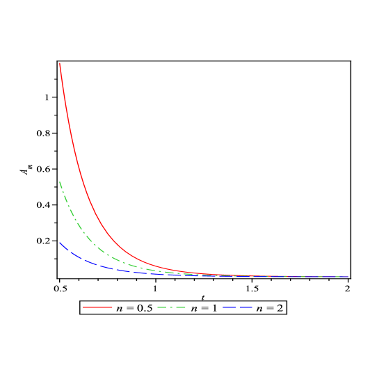
Figure 1: The anisotropic parameter $A_{m}$ versus $t$. Here $\ell=1$

.

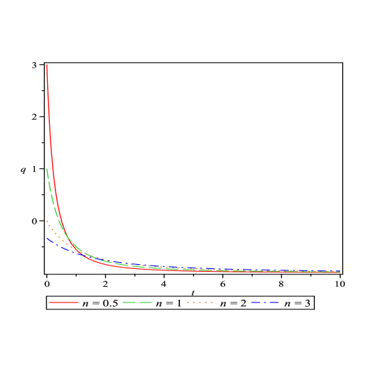
Figure 2: The deceleration parameter $q$ versus $t$

.

Using (31) into (27)-(29), we get the following expressions for scale factors:

$$A(t)=(t^{n}e^{t})^{\frac{1}{2}},$$ (32)

$$B(t)=m(t^{n}e^{t})^{\frac{1}{2}}\exp{\left(\ell\int{(t^{n}e^{t})^{-\frac{3}{2}}dt}\right)},$$ (33)

$$C(t)=m^{-1}(t^{n}e^{t})^{\frac{1}{2}}\exp{\left(-\ell\int{(t^{n}e^{t})^{-\frac{3}{2}}dt}\right)}.$$ (34)

The expressions for physical parameters such as directional Hubble parameters ($H_{x}$, $H_{y}$, $H_{z}$), the Hubble parameter ($H$), scalar of expansion ($\theta$), shear scalar ($\sigma$), spatial volume $V$ and the anisotropy parameter ($A_{m}$) are, respectively, given by

$$H_{x}=\frac{1}{2}\left(\frac{n}{t}+1\right),$$ (35)

$$H_{y}=\frac{1}{2}\left(\frac{n}{t}+1\right)+\ell\left(t^{n}e^{t}\right)^{-\frac{3}{2}},$$ (36)

$$H_{z}=\frac{1}{2}\left(\frac{n}{t}+1\right)-\ell\left(t^{n}e^{t}\right)^{-\frac{3}{2}},$$ (37)

$$\theta=3H=\frac{3}{2}\left(\frac{n}{t}+1\right),$$ (38)

$$\sigma^{2}=\ell^{2}\left(t^{n}e^{t}\right)^{-3},$$ (39)

$$V=\left(t^{n}e^{t}\right)^{\frac{3}{2}}\exp{(2\alpha x)},$$ (40)

$$A_{m}=\frac{8\ell^{2}}{3}\left(\frac{n}{t}+1\right)^{-2}\left(t^{n}e^{t}\right)^{-3}.$$ (41)

It is observed that at $t=0$, the spatial volume vanishes and other parameters $\theta$, $\sigma$, $H$ diverge. Hence the model starts with a big bang singularity at $t=0$. This is a Point Type singularity (MacCallum 1971) since directional scale factor $A(t)$, $B(t)$ and $C(t)$ vanish at initial time.

Figure $1$ depicts the variation of anisotropic parameter ($A_{m}$) versus cosmic time $t$. From the figure, we observe that $A_{m}$ decreases with time and tends to zero as $t\to\infty$ for all values of $n$. Thus, the observed isotropy of the universe can be achieved in our derived model at present epoch. The shear tensor also tends to zero in this model.

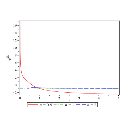
Figure 3: The plot of DE EoS parameter $\omega^{(de)}$ versus $t$. Here $\rho_{0}=1$, $\alpha=1$, $\ell=1$, $\omega^{(m)}=0.5$

.

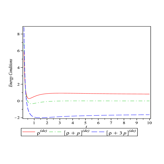
Figure 4: The plot of energy conditions versus $t$ for $n=0.5$. Here $\rho_{0}=1$, $\ell=\alpha=1$, $\omega^{(m)}=0.5$

.

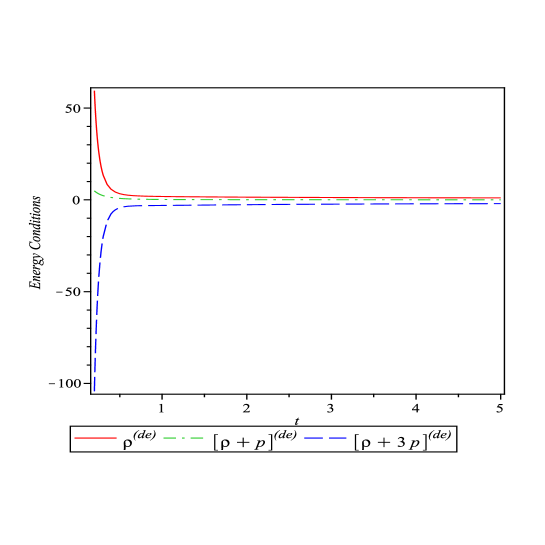
Figure 5: The plot of energy conditions versus $t$ for $n=1$. Here $\rho_{0}=1$, $\ell=\alpha=1$, $\omega^{(m)}=0.5$

.

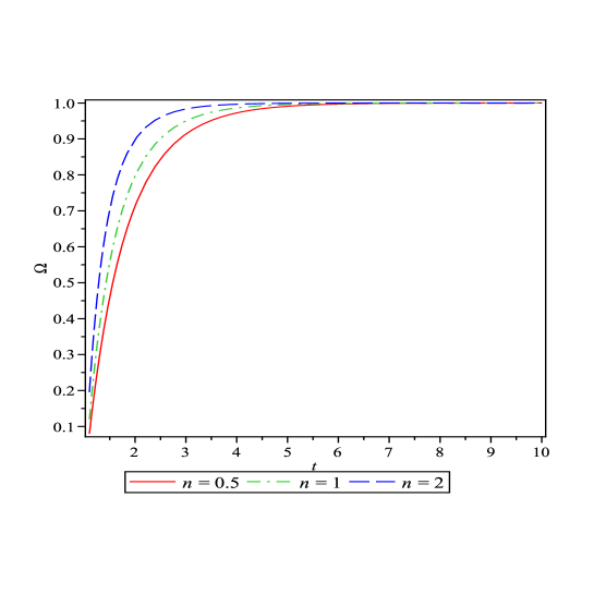
Figure 6: The total energy density parameter $\Omega$ versus $t$. Here $\alpha=\ell=1$

.

We define the deceleration parameter $q$ as usual, i.e.

$$q=-\frac{\ddot{a}a}{\dot{a}^{2}}=-\frac{\ddot{a}}{aH^{2}}.$$ (42)

Using Eq. (31) into Eq. (42), we find

$$q=\frac{2n}{(n+t)^{2}}-1.$$ (43)

From Eq. (43), we observe that $q>0$ for $t<\sqrt{2n}-n$ and $q<0$ for $t>\sqrt{2n}-n$. It is observed that for $0<n<2$, our model is evolving from deceleration phase to acceleration phase. Also, recent observations of SNe Ia, expose that the present universe is accelerating and the value of DP lies to some place in the range $-1<q<0$. It follows that in our derived model, one can choose the value of DP consistent with the observation. Figure $2$ graphs the deceleration parameter ($q$) versus time which gives the behaviour of $q$ from decelerating to accelerating phase for different values of $n$.

The energy density ($\rho^{(m)}$) of perfect fluid, the pressure ($p^{(de)}$) of DE component, DE density ($\rho^{(de)}$) and EoS parameter ($\omega^{(de)}$) of DE, for this model are given by

$$\rho^{(m)}=\rho_{0}(t^{n}e^{t})^{-\frac{3}{2}(1+\omega^{(m)})},$$ (44)

$$p^{(de)}=-\frac{3}{4}\left(\frac{n}{t}+1\right)^{2}+\frac{n}{t^{2}}-\ell(t^{n}e^{t})^{-3}+\alpha^{2}(t^{n}e^{t})^{-1}-\omega^{(m)}\rho_{0}(t^{n}e^{t})^{-\frac{3}{2}(1+\omega^{(m)})},$$ (45)

$$\rho^{(de)}=-\rho_{0}(t^{n}e^{t})^{-\frac{3}{2}(1+\omega^{(m)})}+\frac{3}{4}\left(\frac{n}{t}+1\right)^{2}+\ell(t^{n}e^{t})^{-3}-3\alpha^{2}(t^{n}e^{t})^{-1},$$ (46)

$$\omega^{(de)}=-\frac{\frac{3}{4}\left(\frac{n}{t}+1\right)^{2}-\frac{n}{t^{2}}+\ell(t^{n}e^{t})^{-3}-\alpha^{2}(t^{n}e^{t})^{-1}+\omega^{(m)}\rho_{0}(t^{n}e^{t})^{-\frac{3}{2}(1+\omega^{(m)})}}{\frac{3}{4}\left(\frac{n}{t}+1\right)^{2}+\ell(t^{n}e^{t})^{-3}-3\alpha^{2}(t^{n}e^{t})^{-1}-\rho_{0}(t^{n}e^{t})^{-\frac{3}{2}(1+\omega^{(m)})}}.$$ (47)

Figure $3$ depicts the variation of DE EoS parameter $\omega^{(de)}$ versus cosmic time t. We observe from the figure that for $n<1$, $\omega^{(de)}$ varies from non-dark region crossing the PDL ($\omega^{(de)}=-1$) and ultimately approaches to the phantom region ($\omega^{(de)}<-1$). But for $n\geq 1$, the variation of $\omega^{(de)}$ starts from cosmological constant region ($\omega^{(de)}=-1$) and finally approached to the quintessence region ($\omega^{(de)}>-1$). Therefore, we observe that for $n\geq 1$, the variation of $\omega^{(de)}$ in our derived model is consistent with the recent observations of SNe Ia data [14], SNe Ia data with CMBR anisotropy and galaxy clustering statistics [6].

The dark energy with $\omega^{(de)}<-1$, the phantom component of the universe, leads to uncommon cosmological scenarios as it was pointed out by Caldwell et al. [42]. First of all, there is a violation of the dominant energy condition (DEC), since $\rho+p<0$. The energy density grows up to infinity in a finite time, which leads to a big rip, characterized by a scale factor blowing up in this finite time. These sudden future singularities are, nevertheless, not necessarily produced by a fluid violating DEC. Cosmological solutions for phantom matter which violates the weak energy condition were found by Dabrowski et al. [43]. Caldwell [44], Srivastava [45], Yadav [24] have investigated phantom models with $\omega^{(de)}<-1$ and also suggested that at late time, phantom energy has appeared as a potential DE candidate which violets the weak as well as strong energy condition.

The left hand side of energy conditions have been depicted in Figures $4$ and $5$ for different values of $n$. From Figure $4$, for $n=0.5$ (i.e phantom model) (see, Figure $3$) , we observe that

$$(i)~{}~{}\rho^{(de)}\geq 0,~{}~{}~{}(ii)~{}~{}\rho^{(de)}+p^{(de)}\leq 0,~{}~{}~{}(iii)~{}~{}\rho^{(de)}+3p^{(de)}<0.$$

Thus, from above expressions, we observe the phantom model violates both the strong and weak energy conditions, as expected.

Furthe, from Figure $5$, for $n\geq 1$ (i.e quintessence model) (see, Figure $3$), we observe that

$$(i)~{}~{}\rho^{(de)}\geq 0,~{}~{}~{}(ii)~{}~{}\rho^{(de)}+p^{(de)}\geq 0,~{}~{}~{}(iii)~{}~{}\rho^{(de)}+3p^{(de)}<0.$$

Thus, the quintessence model violates the strong energy condition as the same is predicted by current astronomical observations.

The perfect fluid density parameter ($\Omega^{(m)}$) and DE density parameter ($\Omega^{(de)}$) are given by

$$\Omega^{(m)}=\frac{4}{3}\rho_{0}\left(\frac{n}{t}+1\right)^{2}(t^{n}e^{t})^{-\frac{3}{2}(1+\omega^{(m)})}.$$ (48)

$$\Omega^{(de)}=1+\frac{4}{3}\left(\frac{n}{t}+1\right)^{-2}\left[-\rho_{0}(t^{n}e^{t})^{-\frac{3}{2}(1+\omega^{(m)})}+\ell^{2}(t^{n}e^{t})^{-3}-3\alpha(t^{n}e^{t})^{-1}\right].$$ (49)

Thus the over all density parameter ($\Omega$) is obtained as

$$\Omega=\Omega^{(m)}+\Omega^{(de)}$$

$$=1+\ell^{2}(t^{n}e^{t})^{-3}-3\alpha(t^{n}e^{t})^{-1}.$$ (50)

Figure $6$ depicts the variation of the density parameter ($\Omega$) versus cosmic time $t$ for different values of $n$ during the evolution of the universe. From the Figure $6$, it can be seen that the total energy density $\Omega$ tends to $1$ for sufficiently large time which is supported by the current observations.

4 Cosmic Jerk Parameter

A convenient method to describe models close to $\Lambda$ CDM is based on the cosmic jerk parameter $j$, a dimensionless third derivative of the scale factor with respect to the cosmic time [46]$-$[50]. A deceleration-to-acceleration transition occurs for models with a positive value of $j_{0}$ and negative $q_{0}$. Flat $\Lambda$ CDM models have a constant jerk $j=1$. The jerk parameter in cosmology is defined as the dimensionless third derivative of the scale factor with respect to cosmic time

$$j(t)=\frac{1}{H^{3}}\frac{\dot{\ddot{a}}}{a}.$$ (51)

and in terms of the scale factor to cosmic time

$$j(t)=\frac{(a^{2}H^{2})^{{}^{\prime\prime}}}{2H^{2}}.$$ (52)

where the ‘dots’ and ‘primes’ denote derivatives with respect to cosmic time and scale factor, respectively. One can rewrite Eq. (51) as

$$j(t)=q+2q^{2}-\frac{\dot{q}}{H}.$$ (53)

Eqs. (43) and (53) reduce to

$$j(t)=1-\frac{6n}{(n+t)^{2}}+\frac{8n}{(n+1)^{3}}.$$ (54)

This value overlaps with the value $j\simeq 2.16$ obtained from the combination of three kinematical data sets: the gold sample of type Ia supernovae [9], the SNIa data from the SNLS project [10], and the X-ray galaxy cluster distance measurements [51] for

$$t=3.45\times 10^{-2}A-\frac{50n}{A}-n,$$ (55)

where $A=10^{4}n[8.41+1.45\sqrt{(14.4n+33.6)}]^{\frac{1}{3}}$.

5 Discussion and Concluding Remarks

In this paper, we have studied a spatially homogeneous and anisotropic Bianchi type-V space time filled with perfect fluid and anisotropic DE possessing dynamic energy density. The field equations have been solved exactly with suitable physical assumptions. The solutions satisfy the energy conservation Eq. (17) and the Raychaudhuri Eq. (18) identically. Therefore, exact and physically viable Bianchi type-V model has been obtained. It is to be noted that our procedure of solving the field equations is altogether different from what Kumar & Yadav [25] have adopted. Kumar & Yadav [25] have solved the field equations by considering the constant DP whereas we have considered time dependent DP. As we have already discussed in previous Sect. $3$ that for a Universe which was decelerating in past and accelerating at the present time, the DP must show signature flipping (see the Refs. Padmanabhan and Roychowdhury [38], Amendola [39], Riess et al. [40] and so, there is no scope for a constant DP. The main features of the model are as follows:

$\bullet$ For different values of $n$ the anisotropic parameter $A_{m}$ tends to zero for sufficiently large time. Hence, the present model is isotropic at late time which is consistent to the current observations.

$\bullet$ The present DE model has a transition of the universe from the early deceleration phase to the recent acceleration phase (see, Figure $2$) which is in good agreement with recent observations [52].

$\bullet$ In the present study we find that for $n\geq 1$, the quintessence model is consistent with present and expected future evolution of the universe. The quintessence model approaches to isotropy at late time (see, Figure $1$ & $3$). The other models (for $n<1$), we observe the phantom scenario.

$\bullet$ The derived phantom model violates both the strong and weak energy conditions whereas the quintessence model violates only the strong energy condition (see, Figures $4$ & $5$).

$\bullet$ The total density parameter ($\Omega$) approaches to $1$ for sufficiently large time (see, Figure $6$) which is reproducible with current observations.

$\bullet$ The cosmic jerk parameter in our descended model is also found to be in good agreement with the recent data of astrophysical observations namely the gold sample of type Ia supernovae [9], the SNIa data from the SNLS project [10], and the X-ray galaxy cluster distance measurements [51].

$\bullet$ Our special choice of scale factor yields a time dependent deceleration parameter which represents a model of the Universe which evolves from decelerating phase to an accelerating phase whereas in Yadav [24], Kumar & Yadav [25] only the evolution takes place either in an accelerating or a decelerating phase.

$\bullet$ For different choice of $n$, we can generate a class of DE models in Bianchi type-V space-time. It is observed that such DE models are also in good harmony with current observations. Thus, the solutions demonstrated in this paper may be useful for better understanding of the characteristic of anisotropic DE in the evolution of the universe within the framework of Bianchi type-V space-time.

References

- [1] A. G. Riess et al., Astron. J. 116 1009 (1998).
- [2] S. Perlmutter et al., Astrophys. J. 517 565 (1999).
- [3] T. Padmanabhan, Phys. Rep. 380 235 (2003), arXiv:0603114[astro-ph].
- [4] E. Copeland, M. Sami and S. Tsujikawa, Int. J. Mod. Phys. D 15 1753 (2006), arXiv:0603057[hep-th].
- [5] D. N. Spergel et al., Astrophys. J. Suppl. 148 175 (2003).
- [6] M. Tegmark et al., Phys. Rev. D 69 103501 (2004).
- [7] L. Perivolaropoulos, AIP Conf. Proc. 848 698 (2006), arXiv:0601014[astro-ph].
- [8] H. Jassal, J. Bagla and T. Padmanabhan, Phys. Rev. D 72 103503 (2005), arXiv:0506748[astro-ph].
- [9] A. G. Riess, et al., Astrophys. J. 607 665 (2004).
- [10] P. Astier et al., Astron. Astrophys. 447 31 (2006).
- [11] D. J. Eisentein et al., Astrophys. J. 633 560 (2005).
- [12] C. J. MacTavish et al., Astrophys. J. 647 799 (2006).
- [13] E. Komatsu et al., Astrophys. J. Suppl. Ser. 180 330 (2009).
- [14] R. K. Knop et al., Astrophys. J. 598 102 (2003).
- [15] G. Hinshaw et al., Astrophys. J. Suppl. 180 225 (2009).
- [16] G. Hinshaw et al., Astrophys. J. Suppl. 148 135 (2003).
- [17] G. Hinshaw et al., Astrophys. J. Suppl. 170 288 (2007).
- [18] J. Jaffe et al., Astrophys. J. 629 L1 (2005).
- [19] J. Jaffe et al., Astrophys. J. 643 616 (2006).
- [20] J. Jaffe et al., Astron. Astrophys. 460 393 (2006).
- [21] L. Campanelli and P. Cea, Tedesco, L. Phys. Rev. D 97 131302 (2006).
- [22] L. Campanelli, P. Cea and L. Tedesco, Phys. Rev. D 76 063007 (2007).
- [23] J. Hoftuft et al., Astrophys. J. 699 985 (2009).
- [24] A. K. Yadav, Astrophys. Space Sci. DOI: 10.1007/s10509-011-0745-3 (2011).
- [25] S. Kumar and A. K. Yadav, Mod. Phys. Lett. A 26 647 (2011).
- [26] B. Saha, H. Amirhashchi and A. Pradhan, arXiv:1108.2133 [gr-qc] (2011).
- [27] H. Amirhashchi, A. Pradhan and B. Saha, Chin. Phys. Lett. 28 039801 (2011a), arXiv:1011.3940[gr-qc].
- [28] . Akarsu and C. B. Kilinc, Gen. Relat. Gravit. 42 119 (2010).
- [29] . Akarsu and C. B. Kilinc, Gen. Relat. Gravit. 42 763 (2010).
- [30] . Akarsu and C. B. Kilinc, Astrophys. Space Sci. 42 763 (2010).
- [31] A. Pradhan and H. Amirhashchi, Astrophys. Space Sci. 332, 441 (2011), arXiv:1010.2362[physics.gen-ph].
- [32] H. Amirhashchi, A. Pradhan and H. Zainuddin, Int. J. Theor. Phys. DOI: 10.1007/s10773-011-0861-4 (2011).
- [33] J. L. Tonry, et al., Astrophys. J. 594 1 (2003).
- [34] A. Clocchiatti et al., Astrophys. J. 642 1 (2006).
- [35] C. L. Bennett, et al., Astrophys. J. Suppl. 148 1 (2003).
- [36] P. de Bernardis et al., Nature 404 955 (2000).
- [37] S. Hanany, et al., Astrophys. J. 545 L5 (2000).
- [38] T. Padmanabhan and T. Roychowdhury, Mon. Not. R. Astron. Soc. 344 823 (2003).
- [39] L. Amendola, Mon. Not. R. Astron. Soc. 342 221 (2003).
- [40] A. G. Riess et al.: Astrophys. J. 560 49 (2001).
- [41] M. A. H. MacCallum, Commun. Math. Phys. 20 57 (1971).
- [42] R. R. Caldwell, M. Kamionkowski and N. N. Weinberg, Phys. Rev. Lett. 91 071301 (2003).
- [43] M. P. Dabrowski, T. Stachowiak and M. Szydlowski, Phys. Rev. D 103519 (2003), hep-th/0307128.
- [44] R. R. Caldwell, Phys. Lett. B 545 23 (2002).
- [45] S. K. Srivastava, Phys. Lett. B 619 1 (2005).
- [46] T. Chiba and T. Nakamura, Prog. Theor. Phys. 100 1077 (1998).
- [47] V. Sahni, [arXiv:astro-ph/0211084] (2002).
- [48] R. D. Blandford, M. Amin, E. A. Baltz, K. Mandel and P. L. Marshall, [arXiv:astro-ph/0408279] (2004)
- [49] M. Visser, Class. Quantum Grav. 21 2603 (2004).
- [50] M. Visser, Gen. Relativ. Gravit. 37 1541 (2005).
- [51] D. Rapetti, S. W. Allen, M. A. Amin and R.D. Blandford, Mon. Not. Roy. Astron. Soc. 375 1510 (2007).
- [52] R. R. Caldwell, W. Komp, L. Parker and D. A. T. Vanzella, Phys. Rev. D 73 023513 (2006).