Anomalous long-range correlations at a non-equilibrium phase transition

Abstract

Non-equilibrium diffusive systems are known to exhibit long-range correlations, which decay like the inverse $1/L$ of the system size $L$ in one dimension. Here, taking the example of the $ABC$ model, we show that this size dependence becomes anomalous (the decay becomes a non-integer power of $L$) when the diffusive system approaches a second-order phase transition.

This power-law decay as well as the $L$-dependence of the time-time correlations can be understood in terms of the dynamics of the amplitude of the first Fourier mode of the particle densities. This amplitude evolves according to a Langevin equation in a quartic potential,

which was introduced in a previous work to explain the anomalous behavior of the cumulants of the current near this second-order phase transition. Here we also compute some of the cumulants away from the transition and show that they become singular as the transition is approached.

Introduction

Long range correlations are a well known property of non-equilibrium systems in their steady stateSpohn ; SC ; DKS ; GLMS ; OS ; DELO ; BDGJL-cor . For one dimensional diffusive systems, which satisfy Fourier’s law, these correlations (between pairs of points separated by a macroscopic distance) scale like the inverse $1/L$ of the system size $L$Spohn ; BDGJL-cor ; DLS5 . They can also be related to the non local nature of the the large deviation functional of the density profilesBDGJL-cor ; derrida2007 .

These long range correlations have been calculated in a few cases, using in particular fluctuating hydrodynamicsSpohn ; GLMS ; DELO ; BDLV . It was observed that when a diffusive system approaches a second order phase transition, the factor in front of these $1/L$ correlations becomes singularBDLV . The goal of the present work is to analyse these long range correlations at and in the neighborhood of a phase transition. To do so, we consider the $ABC$ model, one of the simplest diffusive systems which undergoes a phase transition.

The main result obtained in the present work is that the long range correlations at the second-order phase transition of the $ABC$ model have an anomalous dependence on the system size which can be understood by an effective theory GD for the amplitude of the slow density mode which becomes unstable at the transition.

This effective theory, which was developed in a recent work GD , led us to predict an anomalous size dependence of the cumulants of the particle current at the transition. Here, we also show that, away from the transition, these cumulants satisfy Fourier’s law (i.e. are proportional to $1/L$), with prefactors which become singular at the transition.

The outline of the paper is as follows: in section I, we first recall some known properties of the $ABC$ model as well as our previous resultsGD on the cumulants of the current, which exhibit an anomalous Fourier’s law at the second-order transition. In sections II and III, we show how the effective theory for the slow density mode yields a $L^{-1/2}$ size dependence of the correlation function in the critical regime. In section IV, we calculate the cumulants of the particle current (all the cumulants in the flat phase and the first two cumulants in the modulated phase). They all decay like $1/L$, with prefactors which become singular at the transition, and which match the expressions obtained directly in the critical regime in GD .

I Short review of the ABC model

The $ABC$ model is a one-dimensional lattice gas, where each site is occupied by one of three types of particles, $A$, $B$ or $C$. Neighboring sites exchange particles at the rates

$$AB \underset{1}{\overset{q}{\rightleftharpoons}}BA$$

$$BC \underset{1}{\overset{q}{\rightleftharpoons}}CB$$ (1)

$$CA \underset{1}{\overset{q}{\rightleftharpoons}}AC$$

with an asymmetry $q\leq 1$. This model has been studied on a closed and on an open interval (with particle reservoirs at each end)ACLMMS ; LM ; LCM ; BLS as well as on a ring with periodic boundary conditionsEKKM1 ; EKKM2 ; CDE ; FF1 ; FF2 ; CM ; BCP ; BD ; GMS : in this article, we consider the latter case by studying a ring of $L$ sites.

For $q=1$, all configurations are equally likely in the steady state; on the other hand, for $q<1$, the particles of the same species tend to gather EKKM1 . When $q$ scales as

$$q=e^{-\beta/L}\,,$$

the dynamics of the model becomes diffusiveHS ; BDGJL3 : for each species $a\in\{A,B,C\}$, one can define a rescaled density profile $\rho_{a}$,

$${\rm Pro}[\mbox{site }k\mbox{ is of type }a]=\rho_{a}(k/L,t/L^{2})\equiv\rho_{a}(x,\tau)\,.$$ (2)

Because the microscopic dynamics (1) conserves the numbers of particles, the $\rho_{a}(x,\tau)$ are related to their associated currents $j_{a}(x,\tau)$ by the conservation laws

$$\partial_{t}\rho_{a}(x,\tau)=-\partial_{x}j_{a}(x,\tau)\,.$$ (3)

By assuming that the underlying microscopic regions of the system are local equilibrium CDE ; BDLV ; BD2005 , one can show that the currents $j_{a}(x,\tau)$ satisfy noisy, biased Fick’s laws:

$$j_{a}=-\partial_{x}\rho_{a}+\beta\rho_{a}(\rho_{c}-\rho_{b})+{1\over\sqrt{L}}\eta_{a}(x,\tau)$$ (4)

where $b$ and $c$ designate the previous and next species with respect to $a$, and where the $\eta_{a}(x,\tau)$ are Gaussian white noises such that

$$\left\langle\eta_{a}(x,\tau)\eta_{a^{\prime}}(x^{\prime},\tau^{\prime})\right\rangle=\sigma_{aa^{\prime}}\delta(x-x^{\prime})\delta(\tau-\tau^{\prime})\\ \mbox{ with }\sigma_{aa^{\prime}}=\left\{\begin{array}[]{ll}2\rho_{a}(1-\rho_{a})&\mbox{ if }a=a^{\prime}\\ -2\rho_{a}\rho_{a^{\prime}}&\mbox{ otherwise}\end{array}\right.$$

(note that these correlations imply $\eta_{A}+\eta_{B}+\eta_{C}=0$ due to the fact that $j_{A}+j_{B}+j_{C}$ is identically zero). At leading order in $L$, the noise in (4) can be neglected, so that (3) leads to the evolution equationsCDE

$$\partial_{\tau}\rho_{a}=\partial_{x}^{2}\rho_{a}+\beta\partial_{x}\rho_{a}(\rho_{b}-\rho_{c})\,.$$ (5)

For low $\beta$, the flat density profiles $\rho_{a}(x,\tau)=r_{a}$ are a stable solution of these equations. They become linearly unstableEKKM1 ; CDE ; CM when $\beta$ reaches $\beta_{*}$ given by

$$\beta_{*}={2\pi\over\sqrt{\Delta}}\;\;\mbox{ with }\;\;\Delta=1-2\sum_{a}r_{a}^{2}\,`,$$

indicating a second-order transition at $\beta=\beta_{*}$ : above $\beta_{*}$, the steady-state profiles are modulated. It has been argued that these steady-state density profiles are time-independentCM ; BD .

This stability analysis does not rule out the possibility of a first-order phase transition taking place at some $\beta_{t}<\beta_{*}$. A more detailed analysis of the neighborhood of $\beta_{*}$ shows that for $\Lambda<0$, the transition should be first orderCDE , with

$$\Lambda=\sum r_{a}^{2}-2\sum r_{a}^{3}\,.$$ (6)

While no analytical expression for $\beta_{t}$ is known in this case, it has been studied numerically in CM .

In GD , we considered the $ABC$ model in the region $\Lambda>0$ where the transition is expected to be second order. We found that, for a system of size $L$, there exists a critical regime $|\beta-\beta_{*}|\sim 1/\sqrt{L}$ for which the dynamics of the density profiles is dominated by those of their first Fourier mode. Let

$$R_{A}(t)={1\over L}\sum_{k=1}^{L}{\rm e}^{-2{\rm i}\pi k/L}A_{k}(t)\mbox{ where }A_{k}(t)=\left\{\begin{aligned} 1&\mbox{ if site }k\mbox{ is of type }A\\ 0&\mbox{ otherwise}\end{aligned}\right.$$ (7)

be the first Fourier mode of the density of species $A$. Then, near the transition, the first Fourier modes of the other densities, $R_{B}(t)$ and $R_{C}(t)$, are related to $R_{A}$ by

$$\left\{\begin{array}[]{l}R_{B}(t)={2r_{C}-1-{\rm i}\sqrt{\Delta}\over 2r_{A}}R_{A}(t)\\ R_{C}(t)={2r_{B}-1+{\rm i}\sqrt{\Delta}\over 2r_{A}}R_{A}(t)\end{array}\right.\,,$$ (8)

and the evolution of $R_{A}(t)$ can be described by a Langevin equation in a quartic potential in terms of the diffusive time $\tau=t/L^{2}$:

$${{\rm d}R_{A}\over{\rm d}\tau}=4\pi^{2}\left[\gamma-{2\Lambda\over r_{A}\Delta^{2}}|R_{A}|^{2}\right]R_{A}+{\mu_{A}(\tau)\over\sqrt{L}}$$ (9)

with

$$\gamma={\beta-\beta_{*}\over\beta_{*}}$$

and with $\mu_{A}$ is a complex Gaussian white noise:

$$\left\langle\mu_{A}(\bar{\tau})\mu_{A}^{*}(\bar{\tau}^{\prime})\right\rangle=24\pi^{2}{r_{A}^{2}r_{B}r_{C}\over\Delta}\delta(\tau-\tau^{\prime})\,.$$

By rescaling $R_{A}(\tau)$ by

$$R_{A}(\tau)=\left[\Delta r_{A}^{3}r_{B}r_{C}\over\Lambda L\right]^{1/4}f(\bar{\tau})\,,$$ (10)

one can see that (9) becomes

$${{\rm d}f\over{\rm d}\bar{\tau}}=(\bar{\gamma}-|f(\bar{\tau})|^{2})f(\bar{\tau})+\mu(\bar{\tau})\,,$$ (11)

where $\left\langle\mu(\bar{\tau})\mu^{*}(\bar{\tau}^{\prime})\right\rangle=\delta(\bar{\tau}-\bar{\tau}^{\prime})$ and with

$$\bar{\tau}=8\pi^{2}{\sqrt{3\Lambda r_{A}r_{B}r_{C}}\over\Delta^{3/2}}{t\over L^{5/2}}\mbox{ and }\bar{\gamma}=\sqrt{L}{\Delta^{3/2}\over 2\sqrt{3\Lambda r_{A}r_{B}r_{C}}}{\beta-\beta_{*}\over\beta_{*}}\,.$$ (12)

Hence, in the critical regime $|\beta-\beta_{*}|\simeq 1/\sqrt{L}$, the amplitude $R_{A}$ of the first Fourier mode varies on a time scale $\bar{\tau}\propto t/L^{5/2}$, with an amplitude in $1/L^{1/4}$.

In GD , we showed that, due to these slow fluctuations of $R_{A}(t)$, the integrated particle current $Q_{A}(t)$ of $A$ particles during time $t$ through a section in the system exhibits anomalous fluctuations at the transitions, reminiscent of those that can be numerically observed in momentum-conserving mechanical modelsBDG :

$$\left\langle Q_{A}(t)\right\rangle \simeq{t\over L}\beta r_{A}(r_{C}-r_{B})+{t\over L^{3/2}}A_{1}$$ (13)

$$\left\langle Q_{A}^{n}(t)\right\rangle \simeq{t\over L^{5/2-n}}A_{n}\mbox{ for }n\geq 2\,.$$

We also argued that the coefficients $A_{n}$ can be expressed in terms of $n$-point correlation functions of the solution $f(\bar{\tau})$ of (11):

$$C_{n}(\bar{\gamma})=\lim_{\bar{\tau}\to\infty}{1\over\bar{\tau}}\int_{0}^{\bar{\tau}}d\bar{\tau}_{1}..d\bar{\tau}_{n}\left\langle|f(\bar{\tau}_{1})..f(\bar{\tau}_{n})|^{2}\right\rangle_{c}\,.$$ (14)

Therefore in GD we reduced the calculations of the cumulants of $Q_{A}(t)$ in the critical regime to the study of the Langevin equation of a single particle evolving in a quartic potential.

II Power-law relaxation of the first Fourier mode

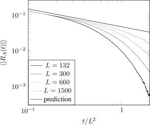
Figure 1: Relaxation of the first-mode amplitude $|R_{A}(t)|$ measured using (7) for systems of size $132\leq L\leq 1500$ started in a segregated initial configuration, for $r_{A}=r_{B}=r_{C}=1/3$ and $\beta=\beta_{*}$. Our analysis (16) of the first mode of the densities predicts a $t^{-1/2}$ decay (see (16)).

In this section, we study the decay of the first Fourier mode in the critical regime when its initial amplitude is much larger than its steady-state values $(\sim L^{-1/4})$. This is the case when one starts from a non steady-state initial condition: here we consider such a relaxation, starting from a fully segregated initial configuration of the type $AA..AABB..BBCC..CC$.

According to GD , we expect all the higher Fourier modes of the densities to relax on the hydrodynamic time scale $\tau=t/L^{2}$. After this initial relaxation, the density profiles (2) should be dominated by a first Fourier mode with amplitude $R_{A}(t)$ evolving according to (9),(10); moreover, as long as $R_{A}$ remains much larger than $L^{-1/4}$, the noise term in (9) can be neglected and the evolution of $R_{A}$ reduces to

$${{\rm d}R_{A}\over{\rm d}\tau}=4\pi^{2}\left[\gamma-{2\Lambda\over r_{A}\Delta^{2}}|R_{A}|^{2}\right]R_{A}\,.$$ (15)

When $\beta=\beta_{*}$ (i.e. when $\gamma=0$), $R_{A}$ should thus decay as a power law:

$$R_{A}(\tau)={R_{A}(0)\over\sqrt{1+{16\pi^{2}\Lambda\over r_{A}\Delta^{2}}|R_{A}(0)|^{2}\tau}}\underset{\tau\to\infty}{\simeq}{R_{A}(0)\over|R_{A}(0)|}{\Delta\over 4\pi}\sqrt{r_{A}\over\Lambda\tau}\,.$$ (16)

In Figure 1, we measured numerically the amplitude $|R_{A}|$ from its definition (7) for systems of $132\leq L\leq 1500$ particles for $r_{A}=r_{B}=r_{C}=1/3$ and $\beta=\beta_{*}$. The power-law decay (16) should be valid in a rather limited range of time ($L^{2}\ll t\ll L^{5/2}$), and is rather difficult to observe. Fortunately, the higher Fourier modes seem to relax fast enough for the power-law decay to occur already for $t/L^{2}\simeq 10^{-1}$: our data for increasing sizes seems to converge to the power-law (16) in the whole range $10^{-1}<t/L^{2}<2$.

Figure 1 also shows a departure from this power law at a rescaled time $t/L^{2}$ increasing with $L$ : in the next section, we show that this is due to the increasing effect of the noise term in (9) as $R_{A}$ decreases.

Power-law decay at the tricritical line

The damping term of the evolution equation for $R_{A}$ (15) that we obtained around $\beta=\beta_{*}$ vanishes on the tricritical line $\Lambda=0$ (see eq. (6)). In this case, it is necessary to push the analysis of GD further in order to obtain an effective equation for $R_{A}$. One can show that, when $\Lambda=0$, (15) is replaced by

$${{\rm d}R_{A}\over{\rm d}\tau}=4\pi^{2}\left(\gamma-{|R_{A}|^{4}\over r_{A}^{2}\Delta^{2}}\right)R_{A}\,.$$ (17)

Along this tricritical line ($\gamma=0$, $\Lambda=0$), the $\tau^{-1/2}$ decay of $R_{A}$ in the critical regime (16) should become in $\tau^{-1/4}$.

III Correlations in the steady state

It has been shown that the $ABC$ model exhibits long-range steady-state correlations, scaling as $1/L$, in the flat phase $\beta<\beta_{*}$ BDLV . In the modulated phase $\beta>\beta_{*}$, these correlations should be of order $1$ due to the modulation of the steady-state profiles.

In this section, we show, using our effective dynamics (9),(11) for the first mode $R_{A}$ (9), that these correlations scale as $1/\sqrt{L}$ in the critical regime; we also show that temporal correlations decay on the slow time scale $\bar{\tau}\propto t/L^{5/2}$ at the transition. Finally, we briefly comment on the behavior on the tricritical line $\Lambda=0$.

III.1 Spatial correlations in the critical regime

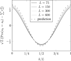
Figure 2: Steady-state density correlations ${\rm Pro}[s_{k}=s_{0}]-\sum r_{a}^{2}$ measured for systems of size $75\leq L\leq 600$, with $r_{A}=r_{B}=r_{C}=1/3$ and $\beta=\beta_{*}$. Our analysis of the first mode of the densities (9) predicts cosine correlations of an amplitude scaling as $1/\sqrt{L}$ (20).

As explained in GD , the density fluctuations in the critical regime are dominated by those of the first Fourier mode $R_{A}$. Thus one can calculate to leading order the steady-state correlations of the densities at the critical point:

$${\rm Pro}[s_{k}=s_{l}]-\sum_{a}r_{a}^{2} \simeq\sum_{a}\left\langle\left(r_{a}+R_{a}{\rm e}^{2{\rm i}\pi k/L}+cc.\right)\left(r_{a}+R_{a}{\rm e}^{2{\rm i}\pi l/L}+cc.\right)\right\rangle_{c}\,.$$

The Langevin equation (11) can be expressed as a Fokker-Planck equation over the probability density of the rescaled first mode $f(\bar{\tau})$,
$P(f_{x},f_{y},\bar{\tau})\equiv{\rm Pro}[f(\bar{\tau})\simeq f_{x}+if_{y}]$ :

$${\partial P\over\partial\bar{\tau}}={\rm div}\left[(r^{2}-\bar{\gamma})P\vec{r}\right]+{1\over 4}{\nabla^{2}}P$$ (18)

with $\vec{r}=(f_{x},f_{y})$ and $\bar{\gamma}$ as defined in (12). From this equation, it is easy to see that $f(\bar{\tau})$ is isotropically distributed in the steady state:

$$P_{0}(\vec{r},\tau)\propto\exp\left[2\bar{\gamma}r^{2}-r^{4}\right]\,.$$

Therefore, $\left\langle R_{a}^{2}\right\rangle=\left\langle R_{a}^{*2}\right\rangle=0$ and

$$\left\langle|R_{a}|^{2}\right\rangle=\sqrt{3\Delta r_{A}^{3}r_{B}r_{C}\over\Lambda L}\left\langle|f^{2}|\right\rangle\mbox{ , with }\left\langle|f^{2}|\right\rangle={\int_{0}^{\infty}r^{3}{\rm e}^{2\bar{\gamma}r^{2}-r^{4}}dr\over\int_{0}^{\infty}r{\rm e}^{2\bar{\gamma}r^{2}-r^{4}}dr}\,.$$

It is easy to compute

$$\left\langle|f|^{2}\right\rangle=\bar{\gamma}+{1\over 2}{{\rm e}^{-\bar{\gamma}^{2}}\over\int_{-\infty}^{\bar{\gamma}}{\rm e}^{-z^{2}}dz}\equiv C_{1}(\bar{\gamma})\,;$$ (19)

this leads to

$${\rm Pro}[s_{k}=s_{l}]-\sum r_{a}^{2}\simeq 2\sqrt{3\Delta r_{a}r_{b}r_{c}\over\Lambda L}C_{1}(\bar{\gamma})\cos 2\pi{k-l\over L}\,.$$ (20)

Therefore, steady-state correlations should scale as $1/\sqrt{L}$ in the critical regime. In Figure 2, we compare our prediction (20) to numerical measurements of systems of $75\leq L\leq 600$ particles, for $\beta=\beta_{*}$ and $r_{A}=r_{B}=r_{C}=1/3$.  
 
Remark: The $\bar{\gamma}\to-\infty$ and $\bar{\gamma}\to+\infty$ limits of our expression for the equal-time correlations (20) can both be checked from known results.

In BDLV , exact expressions for the equal-time density correlations have been calculated in the flat phase (BDLV , eq. (23)): they diverge as $\beta\to\beta_{*}^{-}$, leading to

$${\rm Pro}[s_{k}=s_{l}]-\sum r_{a}^{2}\simeq{6r_{A}r_{B}r_{C}\over\Delta L}{\beta_{*}\over\beta_{*}-\beta}\cos 2\pi{k-l\over L}\,,$$

which is compatible with $C_{1}(\bar{\gamma})\simeq-1/2\bar{\gamma}$ for $\bar{\gamma}\to-\infty$ in (19).

On the other hand, Equation (39) of CDE establishes that the modulated steady-state profiles in the disordered phase are, for $\beta\to\beta_{*}^{+}$, of the form

$$\bar{\rho}_{a}(x)=r_{a}+\Delta\sqrt{{r_{a}\over 2\Lambda}{\beta-\beta_{*}\over\beta_{*}}}{\rm e}^{2{\rm i}\pi(x-\varphi)}+cc.\,,$$

with $x=k/L$ and $\varphi$ an arbitrary phase. This leads to

$${\rm Pro}[s_{k}=s_{l}]-\sum r_{a}^{2}\simeq{\Delta^{2}\over\Lambda}{\beta-\beta_{*}\over\beta_{*}}\cos 2\pi{k-l\over L}\,,$$

which is compatible with $C_{1}(\bar{\gamma})\simeq\bar{\gamma}$ for $\bar{\gamma}\to\infty$ in (19) and (20).

III.2 Decay of the steady-state temporal correlations

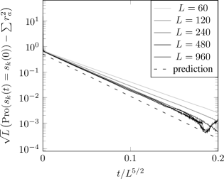
Figure 3: Steady-state time correlations ${\rm Pro}[s_{k}(t)=s_{k}(0)]-\sum r_{a}^{2}$ for systems of size $30\leq L\leq 960$, with $r_{A}=r_{B}=r_{C}=1/3$ and $\beta=\beta_{*}$, as functions of $t/L^{5/2}$. Our effective, fluctuating evolution equation for the first Fourier mode (9) leads us to predict an exponential decay (21).

In the previous section, we have seen that, on a time scale $L^{2}\ll t\ll L^{5/2}$, the first Fourier mode of the densities (7) should decay as a power law when the system relaxes from a non steady state initial configuration. Here we consider the decay of the steady-state density correlations $\left\langle\rho_{a}(x,0)\rho_{a}(x,\tau)\right\rangle_{c}$: the noisy evolution equation (9) implies that they should decay on the ”slow” time scale $t\propto L^{5/2}$. They can be expressed in terms of the rescaled first mode $f(\bar{\tau})$ as

$${\rm Pro}[s_{k}(t)=s_{k}(0)]-\sum r_{a}^{2}\propto{1\over\sqrt{L}}\left\langle f(0)f^{*}(\bar{\tau})+cc.\right\rangle_{c}$$

with $\bar{\tau}\propto\tau/\sqrt{L}$ the rescaled time (12). Let $H_{\bar{\gamma}}$ be the operator of the Fokker-Planck equation (18) over the probability density of $f(\bar{\tau})$, $P(f_{x},f_{y},\bar{\tau})$:

$${\partial P\over\partial\bar{\tau}}\equiv H_{\bar{\gamma}}P\,.$$

For large $\bar{\tau}$, correlations such as $\left\langle f(0)f^{*}(\bar{\tau})\right\rangle_{c}$ should decay as $e^{\lambda_{\bar{\gamma}}\bar{\tau}}$, where $\lambda_{\bar{\gamma}}$ is the second largest eigenvalue of $H_{\bar{\gamma}}$ (the largest being $0$). Thus, we expect time correlations to decay on the time scale $t\propto L^{5/2}$ as

$${\rm Pro}[s_{k}(0)=s_{k}(t)]-\sum r_{a}^{2}\propto{1\over\sqrt{L}}\exp\left[-\alpha{t\over L^{5/2}}\right]$$ (21)

with $\alpha=-8\pi^{2}{\sqrt{3\Lambda r_{A}r_{B}r_{C}}\over\Delta^{3/2}}\lambda_{\bar{\gamma}}$. While there is no known analytical expression for $\lambda_{\bar{\gamma}}$, one can determine it numerically by approximating the operator $H_{\bar{\gamma}}$ over a finite subspace of $L^{2}({\mathbb{R}}^{2})$ of growing dimension. Because the steady-state (and thus the $0$-eigenvector of $H_{\bar{\gamma}}$) is $P_{0}(f_{x},f_{y})\propto e^{2\bar{\gamma}\vec{r}^{2}-\vec{r}^{4}}$, we consider the subspace

$$P_{Q}(f_{x},f_{y})=Q(f_{x},f_{y}){\rm e}^{2\bar{\gamma}r^{2}-r^{4}}\,,$$

where $Q(f_{x},f_{y})$ is a polynomial of degree less than some finite $N$ in $(f_{x},f_{y})$. We need to define a scalar product $\left\langle\cdot|\cdot\right\rangle$ for which $H_{\bar{\gamma}}$ is Hermitian: to do so, we choose

$$\left\langle P_{Q}|P_{R}\right\rangle =\iint dxdy{\rm e}^{r^{4}-2\bar{\gamma}r^{2}}P_{Q}(x,y)P_{R}(x,y)$$ (22)

$$=\iint dxdy{\rm e}^{2\bar{\gamma}r^{2}-r^{4}}Q(x,y)R(x,y)\,,$$

for which the matrix elements of $H_{\bar{\gamma}}$ read

$$\left\langle P_{Q}|H_{\bar{\gamma}}|P_{R}\right\rangle=-{1\over 4}\iint dxdy{\rm e}^{2\bar{\gamma}r^{2}-r^{4}}(\vec{\nabla}Q).(\vec{\nabla}R)\,.$$ (23)

For $\bar{\gamma}=0$, we constructed an orthonormal basis of the subspace of the $P_{Q}$ with respect to the scalar product (22) for $2\leq N\leq 8$; then, we computed the matrix elements of $H_{0}$ (23) in this basis. The second largest eigenvalue of these successive hermitian matrices appears to converge to

$$\lambda_{0}\simeq-0.83\,.$$

In Figure 3, we compare this prediction with the results of simulations in the steady-state for $60\leq L\leq 960$, $r_{A}=r_{B}=r_{C}=1/3$ and $\beta=\beta_{*}$.

The exponential decay (21) also seems to predict the cut-off of the power law decay of Figure 1 observed in systems relaxing from an arbitrary initial condition to the stationary state.

III.3 Correlations on the tricritical line

As in the deterministic case the cubic term of the fluctuating evolution equation for the first Fourier mode (9) vanishes on the tricritical line $\Lambda=0$. The fluctuating correction of the deterministic tri-critical evolution equation (17) is the same as those of (9) :

$${{\rm d}R_{A}\over{\rm d}\tau}=4\pi^{2}\left(\gamma-{|R_{A}|^{4}\over r_{A}^{2}\Delta}\right)R_{A}+{\mu_{A}\over\sqrt{L}}\,.$$

This leads to the rescaling

$$R_{a}={\sqrt[3]{6r_{a}^{4}r_{b}r_{c}}\over L^{1/6}}g(\tilde{\tau})\mbox{ with }{{\rm d}g\over{\rm d}\tilde{\tau}}=(\tilde{\gamma}-|g|^{4})g+\mu(\tilde{\tau})\,,$$

with

$$\tilde{\tau}={4\pi^{2}\over\Delta}(6r_{a}r_{b}r_{c})^{2/3}{t\over L^{8/3}}\mbox{ and }\tilde{\gamma}={\Delta\over(6r_{a}r_{b}r_{c})^{2/3}}L^{2/3}{\beta-\beta_{*}\over\beta_{*}}\,.$$

Hence, the tricritical regime occurs for $|\beta-\beta_{*}|\propto L^{-2/3}$ : it is characterized by fluctuations of the first Fourier mode of amplitude $L^{-1/6}$ on a time scale $t\propto L^{8/3}$.

In its steady state, we expect spatial correlations to scale as

$${\rm Pro}[s_{k}(t)=s_{l}(t)]-\sum r_{a}^{2}\propto{1\over L^{1/3}}\cos 2\pi{k-l\over L}\,,$$

while time correlations should decay exponentially on the time scale $t\propto L^{8/3}$, as

$${\rm Pro}[s_{k}(0)=s_{k}(t)]-\sum r_{a}^{2}\propto{1\over L^{1/3}}\exp\left[-\alpha{t\over L^{8/3}}\right]\,.$$

IV Fluctuations of the current in the $ABC$ model

In this section, we study the cumulants of the integrated current of particles of type $A$, $Q_{A}(t)$, as $\beta\to\beta_{*}$.

In contrast to GD , where we studied the critical regime $|\beta-\beta_{*}|\sim 1/\sqrt{L}$, here we compute the cumulants to leading order in $L$ for a fixed $\beta\neq\beta_{*}$: the expressions we obtain diverge at $\beta_{*}$. For $\beta\to\beta_{*}^{-}$ , we find (37)

$$\left\{\begin{array}[]{ll}{\left\langle Q_{A}(t)\right\rangle\over t}&\simeq{A_{1}\over L}+{B_{1}\over L^{2}(\beta-\beta_{*})}\\ {\left\langle Q_{A}^{2}(t)\right\rangle_{c}\over t}&\simeq{A_{2}\over L}+{B_{2}\over L^{2}(\beta-\beta_{*})^{3}}\end{array}\right.\mbox{ and }{\left\langle Q_{A}^{n}(t)\right\rangle_{c}\over t}\simeq{B_{n}\over L^{2}(\beta-\beta_{*})^{2n-1}}$$ (24)

while we find that, for $\beta\to\beta_{*}^{+}$ (35),

$${\left\langle Q_{A}^{2}(t)\right\rangle_{c}\over t}\simeq{B^{\prime}_{2}\over L(\beta-\beta_{*})}\,.$$

We also show that these expressions are compatible with the $\bar{\gamma}\to\pm\infty$ limits of the expressions of the cumulants (38),(39) in terms of the functions $C_{n}(\bar{\gamma})$ (14) derived in the critical regime in GD .

IV.1 First cumulant of the current

We start with the assumption that the steady state density profiles $\bar{\rho}_{a}(x)$, which are the long-time limits of the leading-order, deterministic hydrodynamic equations (5), are time-independent, both in the flat and in the modulated phase. The associated particle currents $j_{a}$ are thus homogeneous, $j_{a}(x,\tau)=J_{a}$, and can be computed by integrating (4) in space, yielding

$$J_{a}=\int_{0}^{1}\beta\bar{\rho}_{a}(x)(\bar{\rho}_{c}(x)-\bar{\rho}_{b}(x))dx\,.$$ (25)

Then, the average integrated current $\left\langle Q_{A}(t)\right\rangle$ through any position in the system will behave in the long-time limit like $\left\langle Q_{A}(t)\right\rangle\simeq{t\over L}J_{A}$, so that

$${\left\langle Q_{A}(t)\right\rangle\over t}\simeq{1\over L}\int_{0}^{1}\beta\bar{\rho}_{A}(x)(\bar{\rho}_{C}(x)-\bar{\rho}_{B}(x))dx\,.$$

For $\beta<\beta_{*}$, we thus obtain ${\left\langle Q_{A}(t)\right\rangle}\simeq{t\over L}\beta r_{A}(r_{C}-r_{B})$. For $\beta>\beta_{*}$, the analytic expression of the $\bar{\rho}_{a}(x)$ is rather complicatedCM . However, their limit as $\beta\to\beta_{*}^{+}$ takes a simple form (see CDE , or the $\bar{\gamma}\to\infty$ limit of (9)):

$$\bar{\rho}_{a}(x)\underset{\beta\downarrow\beta_{*}}{\simeq}r_{a}+(R_{a}{\rm e}^{2{\rm i}\pi x}+cc.)$$ (26)

with $|R_{A}|=\Delta\sqrt{r_{A}(\beta-\beta_{*})/2\Lambda\beta_{*}}$ and with $R_{B}$, $R_{C}$ related to $R_{A}$ by (8). This leads to an analytical expression for $\left\langle Q_{A}(t)\right\rangle$ when $\beta\to\beta_{*}^{+}$ :

$${\left\langle Q_{A}(t)\right\rangle\over t}\underset{\beta\downarrow\beta_{*}}{\simeq}{r_{C}-r_{B}\over L}\left[\beta r_{A}-{\Delta^{2}\over\Lambda}(\beta-\beta_{*})\right]\,.$$

IV.2 Second cumulant of the current

In order to compute fluctuations of the current $Q_{A}(t)$, the noise terms of the biaised Fick’s law (4) have to be taken into account. These fluctuating hydrodynamics can be reformulated as a large deviation principle known as the macroscopic fluctuation theory (MFT)BDGJL1 ; BDGJL2 ; BDGJL5 ; BD ; BDLV , which gives the probability of observing a given evolution $\rho_{a}(x,\tau)$ of the density profiles :

$${\rm Pro}[\rho_{a}(x,\tau)]\propto\exp\left[-L\iint dxd\tau{1\over 2}(j-q).\sigma^{-1}(j-q)\right]$$ (27)

where $j=(j_{A},j_{B})$, $q=(q_{A},q_{B})$ (with $q_{a}=-\partial_{x}\rho_{a}+\beta\rho_{a}(\rho_{c}-\rho_{b})$ the deterministic part of (4)) and with

$$\sigma=\left(\begin{array}[]{rr}\sigma_{AA}&\sigma_{AB}\\ \sigma_{BA}&\sigma_{BB}\\ \end{array}\right)=2\left(\begin{array}[]{rr}\rho_{A}(1-\rho_{A})&-\rho_{A}\rho_{B}\\ -\rho_{A}\rho_{B}&\rho_{B}(1-\rho_{B})\\ \end{array}\right)\,.$$

The generating function $\log\left\langle e^{\lambda Q_{A}(t)}\right\rangle$ can then be calculated as the solution of a variational problem :

$$\log\left\langle e^{\lambda Q_{A}(t)}\right\rangle=\max_{\rho_{a},j_{a}}L\int_{0}^{t/L^{2}}d\tau\int_{0}^{1}dx\left[\lambda j_{A}-{1\over 2}(j-q).\sigma^{-1}(j-q)\right]\,.$$ (28)

For $\lambda=0$, the optimum in the above is the solution to the deterministic equations (5), which satisfy by definition $j=q$ : these are $\rho_{a}(x,\tau)=r_{a}$ (for $\beta\leq\beta_{*}$) or $\rho_{a}(x,\tau)=\bar{\rho}_{a}(x)$ (for $\beta>\beta_{*}$), and $j_{a}(x,\tau)=J_{a}$ defined by (25).

For $\beta<\beta_{*}$, the optimal profiles are still flat even for $\lambda\neq 0$ (as we will see below, they are a stable minimum):

$$\left\{\begin{aligned} \rho(x,\tau)&=r\\ j(x,\tau)&=q+\sigma\left(\begin{array}[]{r}\lambda\\ 0\end{array}\right)\equiv J(\lambda)\end{aligned}\right.$$ (29)

with $\rho=(\rho_{A},\rho_{B})$, $r=(r_{A},r_{B})$, and $q$ and $\sigma$ taking their constant values for $\rho=r$. This leads to

$$\log\left\langle e^{\lambda Q_{A}(t)}\right\rangle\underset{\beta<\beta_{*}}{\simeq}{t\over L}\left[\beta\lambda r_{A}(r_{C}-r_{B})+\lambda^{2}r_{A}(1-r_{A})\right]\equiv{t\over L}F_{\rm flat}(\lambda)$$ (30)

and to

$${\left\langle Q_{A}^{2}(t)\right\rangle_{c}\over t}\simeq{2\over L}r_{A}(1-r_{A})\mbox{ and }{\left\langle Q_{A}^{n}(t)\right\rangle_{c}\over t}=o\left(1\over L\right)\mbox{ for }n\geq 3\,.$$ (31)

On the other hand, the optimal profiles in (28) vary with $\lambda$ for $\beta>\beta_{*}$, with non-trivial optimization equations. We will therefore restrict ourselves to the calculation of $\left\langle Q_{A}^{2}(t)\right\rangle$, for which it is sufficient to compute (28) to second order in $\lambda$.

In order to do so, we consider profiles close to the $\lambda=0$ optimum, $\rho_{a}=\bar{\rho}_{a}(x)$ and $j_{a}=J_{a}$. Because arbitrary translations of these profiles are also optimal, we need to consider profiles moving at a small velocity $v$ : this amounts to

$$\left\{\begin{aligned} \rho(x,t)&=\bar{\rho}(x-vt)+\mu(x-vt)\\ j(x,t)&=J+K-v\bar{\rho}(x-vt)\end{aligned}\right.$$

with $\rho=(\rho_{A},\rho_{B})$ and $\mu(x),v,K\ll 1$. Because $q_{a}=-\partial_{x}\rho_{a}+\beta\rho_{a}(\rho_{c}-\rho_{b})$, this leads to the following expression for $q$ :

$$q=\bar{q}-\mu^{\prime}-\bar{M}\mu\mbox{ with }\bar{M}=\beta\left(\begin{array}[]{rr}1-2\bar{\rho}_{C}&2\bar{\rho}_{A}\\ -2\bar{\rho}_{B}&2\bar{\rho}_{C}-1\end{array}\right)\,,$$

$\bar{q}=q(\bar{\rho})$ and $\mu^{\prime}=\partial_{x}\mu$. Then, the right-hand side of (28) becomes

$$S=\max_{K,v,\mu(x)}{t\over L}\int dx\left[\lambda(\bar{J}_{A}+K_{A}-v\bar{\rho}_{A})\right.\\ \left.-{1\over 2}(K-v\bar{\rho}+\mu^{\prime}+\bar{M}\mu).\bar{\sigma}^{-1}(K-v\bar{\rho}+\mu^{\prime}+\bar{M}\mu)\right]$$ (32)

with $\bar{\sigma}=\sigma(\bar{\rho})$. The optimization equations over $K$, $v$ and $\mu$ can be written as

$$\left\{\begin{aligned} \int dxF&=\left(\begin{array}[]{r}\lambda\\ 0\end{array}\right)\\ \int dx\bar{\rho}.F&=\lambda r_{A}\\ F^{\prime}&=\bar{M}^{T}F\end{aligned}\right.$$ (33)

with $F=\bar{\sigma}^{-1}(K-v\bar{\rho}+\mu^{\prime}+\bar{M}\mu)$. The right-hand side of (28) then reads

$$S=\max_{K,v,F(x)}{t\over L}\int dx\left[\lambda(\bar{J}_{A}+K_{A}-v\bar{\rho}_{A})-{1\over 2}F.\bar{\sigma}F\right]$$

It can be expressed completely in terms of the optimal $F(x)$ solution of (33) by using

$$\int dxF.\bar{\sigma}F =\int F.(K-v\bar{\rho}+\mu^{\prime}+\bar{M}\mu)$$

$$=K.\int dxF-v\int dx\bar{\rho}.F+\int dx\mu.(\bar{M}^{T}F-F^{\prime})$$

$$=\lambda(K_{A}-vr_{A})$$

so that the generating function is given to second order in $\lambda$ by

$$\log\left\langle e^{\lambda Q_{A}(t)}\right\rangle\simeq{t\over L}\int dx\left[\lambda\bar{J}_{A}+{1\over 2}F.\bar{\sigma}F\right]$$ (34)

By determining the solution $F(x)$ of (33) and integrating (34) numerically, $\left\langle Q_{A}^{2}(t)\right\rangle_{c}$ can be predicted to leading order in $L$ for $\beta>\beta_{*}$. This prediction diverges as $\beta\to\beta_{*}^{+}$ : because $\bar{\rho}(x)$ is known analytically in this limit (26), we were able to calculate $F(x)$ exactly,

$$F(x)={4\pi\lambda(r_{B}-r_{C})\over\Delta^{3/2}(\beta-\beta_{*})}\left(\begin{aligned} R_{B}\\ -R_{A}\end{aligned}\right){\rm e}^{2{\rm i}\pi x}+cc.+{\mathcal{O}}(1)\,,$$

leading to a simple expression for $\left\langle Q_{A}^{2}(t)\right\rangle_{c}$ in this limit:

$$\left\langle Q_{A}^{2}(t)\right\rangle_{c}\underset{\beta\downarrow\beta_{*}}{\simeq}{t\over L}{12\pi r_{A}r_{B}r_{C}(r_{B}-r_{C})^{2}\over\sqrt{\Delta}\Lambda(\beta-\beta_{*})}\,.$$ (35)

IV.3 Higher-order corrections in the flat phase

As shown above, the macroscopic fluctuation theory (28) predicts, for large $L$, Gaussian fluctuations of $Q_{A}(t)$ in the flat phase $\beta<\beta_{*}$, with a non-singular variance (31) as $\beta\to\beta_{*}^{-}$.

Here, we calculate the next $1/L$ corrections to the generating function (30), by generalizing to the $ABC$ model the approach followed in ADLW in the case of a single conserved quantity. These corrections, of order $1/L^{2}$, can be obtained by considering the large-deviation principle (27) as a functional integral :

$$\left\langle e^{\lambda Q_{A}(t)}\right\rangle\propto\int D[\rho_{a}]D[j_{a}]\exp\left[L\iint dxd\tau\left(\lambda j_{A}-{1\over 2}(j-q).\sigma^{-1}(j-q)\right)\right]$$ (36)

where the integral takes place over all profiles $(\rho_{a},j_{a})$ compatible with the conservation law $\partial_{x}j_{a}+\partial_{\tau}\rho_{a}=0$. Fluctuations around the optimum profile (29) then give corrections to the saddle-point expression (30). We now consider such fluctuations, expressing them in terms of their Fourier modes :

$$\left\{\begin{aligned} \rho(x,\tau)&=r+\delta\rho(x,\tau)\\ j(x,\tau)&=J(\lambda)+\delta j(x,\tau)\end{aligned}\right.\mbox{ with }\left\{\begin{aligned} \delta\rho(x,\tau)&=\sum_{k,\omega}k\left[\alpha_{k\omega}{\rm e}^{{\rm i}(kx-\omega t)}+cc.\right]\\ \delta j(x,\tau)&=\sum_{k,\omega}\omega\left[\alpha_{k\omega}{\rm e}^{{\rm i}(kx-\omega t)}+cc.\right]\end{aligned}\right.$$

with $\alpha_{k\omega}=(\alpha_{k\omega}^{(A)},\alpha_{k\omega}^{(B)})$ the amplitude of the fluctuations of wave number $k$ and pulsation $\omega$, which take discrete values :

$$k={2\pi n}\mbox{ with }n\in{\mathbb{N}}^{*}\;\mbox{ and }\;\omega={2\pi m\over t/L^{2}}\mbox{ with }m\in{\mathbb{Z}}\,.$$

Expanding (36) to second order in the $\alpha_{k\omega}$, we obtain

$$\left\langle e^{\lambda Q_{A}(t)}\right\rangle\propto\int\left[\prod_{k,\omega}d\alpha_{k\omega}d\alpha_{k\omega}^{*}\right]\exp\left[{t\over L}F_{\rm flat}(\lambda)-\sum_{k,\omega}\alpha_{k\omega}^{*}.M_{k\omega}\alpha_{k\omega}\right]$$

with $F_{\rm flat}(\lambda)$ the dominant-order generating function (30) and
$M_{k\omega}={1\over 2}\left(\begin{array}[]{cc}\phi_{A}+\phi_{C}&\phi_{C}-6{\rm i}\beta k^{3}\\ \phi_{C}+6{\rm i}\beta k^{3}&\phi_{B}+\phi_{C}\end{array}\right)$, with

$$\phi_{a}={(J_{a}(\lambda)k-\omega r_{a})^{2}\over r_{a}^{3}}+{k^{4}\over r_{a}}+\beta^{2}k^{2}(4-9r_{a})\,.$$

Integrating the Gaussian variables $\alpha_{k\omega}$ gives the corrections

$$\log\left\langle e^{\lambda Q_{A}(t)}\right\rangle\simeq{t\over L}F_{\rm flat}(\lambda)-\sum_{k,\omega}\log P_{k}(\lambda,\omega)+C$$

with $P_{k}(\lambda,\omega)=\phi_{A}\phi_{B}+\phi_{B}\phi_{C}+\phi_{C}\phi_{A}-36\beta^{2}k^{6}$ and $C$ an additive constant fixed by the condition $\log\left\langle e^{\lambda Q_{t}}\right\rangle=0$ for $\lambda=0$. In the $t\to\infty$ limit, the sum over $\omega$ can be replaced by an integral :

$$\log\left\langle e^{\lambda Q_{A}(t)}\right\rangle\simeq{t\over L}F_{\rm flat}(\lambda)-{t\over 2\pi L^{2}}\sum_{k}\int d\omega\log P_{k}(\lambda,\omega)+C\,.$$

Because only the first mode of the fluctuations, $k=2\pi$, becomes unstable as $\beta\to\beta_{*}^{-}$, we expect the divergence in the cumulants at the transition to only affect this $k=2\pi$ term. Thus we take the following limit in $P_{2\pi}(\lambda,\omega)$ : $\lambda\simeq 0$ (to determine the cumulants), $\omega\simeq 0$ (we expect slow fluctuations to be responsible for the divergence), and $\beta\simeq\beta_{*}$. Then $P_{2\pi}(\lambda,\omega)$ takes the simplified expression

$$P_{2\pi}(\lambda,\omega)\simeq 64\pi^{4}\left[{\omega^{2}+4\pi^{2}\Delta(\beta-\beta_{*})^{2}\over r_{A}r_{B}r_{C}}+12\beta_{*}^{3}(r_{C}-r_{B})\lambda\right]\equiv Q(\lambda,\omega)\,.$$

The integral of $\log Q(\lambda,\omega)$ is apparently divergent : however, since

$$\int_{-\Omega}^{\Omega}d\omega\log Q(\lambda,\omega)\underset{\Omega\to\infty}{\simeq} 4\Omega\log\Omega$$

$$-4\pi^{2}\sqrt{{\Delta(\beta-\beta_{k})^{2}}+{12k\over\Delta^{3/2}}r_{A}r_{B}r_{C}(r_{B}-r_{C})\lambda}\,,$$

its divergent part is canceled out by adjusting $C$ so that $\log\left\langle e^{\lambda Q_{t}}\right\rangle=0$ for $\lambda=0$. Hence, the part of the generating function which becomes singular as $\beta\to\beta_{*}$ reads

$$\log\left\langle e^{\lambda Q_{A}(t)}\right\rangle\simeq{t\over L}F_{\rm flat}(\lambda)+{4\pi^{2}\gamma t\over L^{2}}\left[\sqrt{1+{24\pi\over\Delta^{5/2}}{r_{A}r_{B}r_{C}\over(\beta-\beta_{*})^{2}}(r_{B}-r_{C})\lambda}-1\right]\,,$$

leading to a divergence of the $n$-th cumulant of $Q_{A}(t)$ scaling as (24), with

$$B_{n}=\sqrt{\Delta\over\pi}\Gamma(n-1/2)\left[{24\pi r_{A}r_{B}r_{C}(r_{C}-r_{B})\over\Delta^{5/2}}\right]^{n}\,.$$ (37)

IV.4 Anomalous fluctuations in the critical regime

In GD , we found that the fluctuations of the first Fourier mode on the slow time scale $\bar{\tau}\propto t/L^{5/2}$ (12) lead to anomalous fluctuations of the integrated current of $Q_{A}(t)$ in the critical regime (13). More precisely, we derived

$$\left\langle Q_{a}(t)\right\rangle \simeq{t\over L}\beta r_{a}(r_{c}-r_{b})+{2t\over L^{3/2}}\beta(r_{b}-r_{c})\sqrt{3\Delta r_{a}r_{b}r_{c}\over\Lambda}C_{1}(\bar{\gamma})$$ (38)

$$\left\langle Q_{a}^{n}(t)\right\rangle_{c} \simeq{t\over L^{5/2-n}}{8\pi^{2}\sqrt{3\Lambda r_{a}r_{b}r_{c}}\over\Delta^{3/2}}\left[\Delta^{3/2}(r_{b}-r_{c})\over 2\pi\Lambda\right]^{n}C_{n}(\bar{\gamma})$$ (39)

with $\bar{\gamma}$ and $C_{n}(\bar{\gamma})$ as defined in (12) and (14). Because $f(\bar{\tau})$ evolves in a quartic potential (11), only $C_{1}(\bar{\gamma})$ can be easily calculated (19). However, (38) and (39) predict the dependence of the cumulants in $(r_{A},r_{B},r_{C},\beta)$ in terms of the unique parameter $\bar{\gamma}$ (12): one can easily check that (37) and (35) are consistent with this dependence, for

$$C_{n}(\bar{\gamma})\underset{\bar{\gamma}\to-\infty}{\simeq}{(-1)^{n}\Gamma(n-1/2)\over 4\sqrt{\pi}\bar{\gamma}^{2n-1}}\mbox{ and }C_{2}(\bar{\gamma})\underset{\bar{\gamma}\to\infty}{\simeq}{2\over\bar{\gamma}}\,.$$

V Conclusion

In this paper we have shown that the long-range correlations (20) of the $ABC$ model near the second-order phase transition decay like the $L^{-1/2}$ power of the system size $L$. In the entire critical regime, these correlations EKKM2 ; BD ; BDG can be understood from the evolution GD of the amplitude of the first Fourier mode given by the Langevin equation of a particle in a quartic potential (11).

We have also computed the cumulants of the current of particles (24) away from the transition, showing that the become singular at the transition in a way which matches the results of our previous work GD where these cumulants were computed in the critical regime.

It would be interesting to see whether other diffusive systems, at a phase transition, display correlation functions and current fluctuations with behaviors similar to those we discovered here for the $ABC$ model.

Deterministic one-dimensional systems, in particular those which conserve momentum, are known to exhibit an anomalous Fourier’s law LLP2 , with cumulants of the current BDG and correlations LMP ; DLLMP ; GDL scaling as a non-integer power of the system size. Although these systems are much more difficult to study than the $ABC$ model (for which one only needs to follow the dynamics of a single mode), it would be interesting to see whether the approximations that have been used so far, such as the mode-coupling approach DLRP ; LuS ; hvB , could predict the power-law dependence of these current and density fluctuations.

Acknowledgments. BD acknowledges the support of the French Ministry of Education through the ANR 2010 BLAN 0108 01 grant.

References

References

- (1) H. Spohn, “Long range correlations for stochastic lattice gases in a non-equilibrium steady state,” J. Phys. A: Math. Gen., vol. 16, p. 4275, 1983.
- (2) R. Schmitz and E. G. D. Cohen, “Fluctuations in a fluid under a stationary heat flux. I. general theory,” J. Stat. Phys., vol. 39, pp. 285–316, 1985.
- (3) J. R. Dorfman, T. R. Kirkpatrick, and J. V. Sengers, “Generic long-range correlations in molecular fluids,” Annu. Rev. Phys. Chem., vol. 45, pp. 213–239, 1994.
- (4) P. L. Garrido, J. L. Lebowitz, C. Maes, and H. Spohn, “Long-range correlations for conservative dynamics,” Phys. Rev. A, vol. 42, pp. 1954–1968, 1990.
- (5) J. M. Ortiz de Zarate and J. V. Sengers, “On the physical origin of long-ranged fluctuations in fluids in thermal nonequilibrium states,” J. Stat. Phys., vol. 115, pp. 1341–1359, 2004.
- (6) B. Derrida, C. Enaud, C. Landim, and S. Olla, “Fluctuations in the weakly asymmetric exclusion process with open boundary conditions,” J. Stat. Phys., vol. 118, pp. 795–811, 2005.
- (7) L. Bertini, A. De Sole, D. Gabrielli, G. Jona-Lasinio, and C. Landim, “On the long range correlations of thermodynamic systems out of equilibrium,” ArXiv:0705.2996, 2007.
- (8) B. Derrida, J. Lebowitz, and E. Speer, “Entropy of open lattice systems,” J. Stat. Phys., vol. 126, pp. 1083–1108, 2007.
- (9) B. Derrida, “Non-equilibrium steady states: fluctuations and large deviations of the density and of the current,” J. Stat. Mech.: Theor. Exp., vol. 2007, p. P07023, 2007.
- (10) T. Bodineau, B. Derrida, V. Lecomte, and F. van Wijland, “Long range correlations and phase transitions in non-equilibrium diffusive systems,” J. Stat. Phys., vol. 133, pp. 1013–1031, 2008.
- (11) Gerschenfeld, A. and Derrida, B., “Current fluctuations at a phase transition,” EPL, vol. 96, p. 20001, 2011.
- (12) A. Ayyer, E. Carlen, J. L. Lebowitz, P. Mohanty, D. Mukamel, and E. R. Speer, “Phase diagram of the ABC model on an interval,” J. Stat. Phys., vol. 137, p. 1166, 2009.
- (13) A. Lederhendler and D. Mukamel, “Long-range correlations and ensemble inequivalence in a generalized ABC model,” Phys. Rev. Lett., vol. 105, no. 15, p. 150602, 2010.
- (14) A. Lederhendler, O. Cohen, and D. Mukamel, “Phase diagram of the ABC model with nonconserving processes,” J. Stat. Mech., no. 11, p. P11016, 2010.
- (15) J. Barton, J. L. Lebowitz, and E. R. Speer, “The grand canonical ABC model: a reflection asymmetric mean-field Potts model,” J. Phys. A: Math. Theor., vol. 44, no. 6, p. 065005, 2011.
- (16) M. R. Evans, Y. Kafri, H. M. Koduvely, and D. Mukamel, “Phase separation and coarsening in one-dimensional driven diffusive systems: Local dynamics leading to long-range hamiltonians,” Phys. Rev. E, vol. 58, no. 3, pp. 2764–2778, 1998.
- (17) M. R. Evans, Y. Kafri, H. M. Koduvely, and D. Mukamel, “Phase separation in one-dimensional driven diffusive systems,” Phys. Rev. Lett., vol. 80, no. 3, pp. 425–429, 1998.
- (18) M. Clincy, B. Derrida, and M. R. Evans, “Phase transition in the ABC model,” Phys. Rev. E, vol. 67, no. 6, p. 066115, 2003.
- (19) G. Fayolle and C. Furtlehner, “Dynamical windings of random walks and exclusion models. part I: Thermodynamic limit in ,” J. Stat. Phys., vol. 114, pp. 229–260, 2004.
- (20) G. Fayolle and C. Furtlehner, “Stochastic dynamics of discrete curves and multi-type exclusion processes,” J. Stat. Phys., vol. 127, pp. 1049–1094, 2007.
- (21) O. Cohen and D. Mukamel, “Phase diagram of the ABC model with nonequal densities,” J. Phys. A: Math. Theor., vol. 44, p. 415004, 2011.
- (22) L. Bertini, N. Cancrini, and G. Posta, “On the Dynamical Behavior of the ABC Model,” arXiv:1104.0822, 2011.
- (23) T. Bodineau and B. Derrida, “Phase fluctuations in the ABC model,” J. Stat. Phys., vol. online first, pp. 1–18.
- (24) G. M. Schütz, “Critical phenomena and universal dynamics in one-dimensional driven diffusive systems with two species of particles,” J. Phys. A: Math. Gen., vol. 36, p. R339, 2003.
- (25) H. Spohn, Large Scale Dynamics of Interacting Particles. Springer-Verlag, 1991.
- (26) L. Bertini, A. De Sole, D. Gabrielli, G. Jona-Lasinio, and C. Landim, “Towards a nonequilibrium thermodynamics: A self-contained macroscopic description of driven diffusive systems,” J. Stat. Phys., vol. 135, pp. 857–872, 2009.
- (27) T. Bodineau and B. Derrida, “Distribution of current in nonequilibrium diffusive systems and phase transitions,” Phys. Rev. E, vol. 72, p. 066110, 2005.
- (28) E. Brunet, B. Derrida, and A. Gerschenfeld, “Fluctuations of the heat flux of a one-dimensional hard particle gas,” EPL, vol. 90, no. 2, p. 20004, 2010.
- (29) L. Bertini, A. De Sole, D. Gabrielli, G. Jona-Lasinio, and C. Landim, “Fluctuations in stationary nonequilibrium states of irreversible processes,” Phys. Rev. Lett., vol. 87, p. 040601, 2001.
- (30) L. Bertini, A. De Sole, D. Gabrielli, G. Jona-Lasinio, and C. Landim, “Macroscopic fluctuation theory for stationary non-equilibrium states,” J. Stat. Phys., vol. 107, pp. 635–675, 2002.
- (31) L. Bertini, A. De Sole, D. Gabrielli, G. Jona-Lasinio, and C. Landim, “Current fluctuations in stochastic lattice gases,” Phys. Rev. Lett., vol. 94, p. 030601, 2005.
- (32) C. Appert-Rolland, B. Derrida, V. Lecomte, and F. van Wijland, “Universal cumulants of the current in diffusive systems on a ring,” Phys. Rev. E, vol. 78, p. 021122, 2008.
- (33) S. Lepri, R. Livi, and A. Politi, “Thermal conduction in classical low-dimensional lattices,” Phys. Rep., vol. 377, pp. 1–80(80), 2003.
- (34) S. Lepri, C. Mejía-Monasterio, and A. Politi, “Nonequilibrium dynamics of a stochastic model of anomalous heat transport,” J. Phys. A: Math. Theor., vol. 43, p. 065002, 2010.
- (35) L. Delfini, S. Lepri, R. Livi, C. Mejía-Monasterio, and A. Politi, “Nonequilibrium dynamics of a stochastic model of anomalous heat transport: numerical analysis,” J. Phys. A: Math. Theor., vol. 43, p. 145001, 2010.
- (36) A. Gerschenfeld, B. Derrida, and J. L. Lebowitz, “Anomalous Fourier’s law and long range correlations in a 1D non-momentum conserving mechanical model,” J. Stat. Phys., vol. 141, pp. 757–766, 2010.
- (37) L. Delfini, S. Lepri, R. Livi, and A. Politi, “Anomalous kinetics and transport from 1D self-consistent mode-coupling theory,” J. Stat. Mech: Theory Exp., no. 02, p. P02007, 2007.
- (38) J. Lukkarinen and H. Spohn, “Anomalous energy transport in the FPU- chain,” Comm. Pure Appl. Math., vol. 61, no. 12, pp. 1753–1786, 2008.
- (39) H. van Beijeren, “Exact results for anomalous transport in one dimensional Hamiltonian systems,” ArXiv:1106.3298, 2011.