Self-organizing magnetic beads for biomedical applications

Abstract

In the field of biomedicine magnetic beads are used for drug delivery and to treat hyperthermia. Here we propose to use self-organized bead structures to isolate circulating tumor cells using lab-on-chip technologies. Typically blood flows past microposts functionalized with antibodies for circulating tumor cells. Creating these microposts with interacting magnetic beads makes it possible to tune the geometry in size, position and shape. We developed a simulation tool that combines micromagnetics and discrete particle dynamics, in order to design micropost arrays made of interacting beads. The simulation takes into account the viscous drag of the blood flow, magnetostatic interactions between the magnetic beads and gradient forces from external aligned magnets. We developed a particle-particle particle-mesh method for effective computation of the magnetic force and torque acting on the particles.

1 Introduction

1.1 Circulating Tumor Cell (CTC)

CTCs detach from a tumor and can remain in the blood even after the tumor is removed. Their presence increases the chance of net tumors developing. It is important to monitor the number of CTCs in the blood but their low concentration (a few per $\mu l$) when compared to normal blood cells (around 5 million per $\mu l$) makes this difficult. A new and flexible method is required.

Lab-on-chips with fixed arrays are designed to use the properties of the CTCs to filter them. The most common ways are mechanical filters or using antibodies. Membranes with slots smaller than tumor cells fulfill the requirements for a mechanical filter [1]. Normal blood cells, they have similar sizes, are more deformable than CTCs and can go through. Another possibility is to use cylindrical posts coated with antibodies [2]. If there is a large surface area the possibility for a connection with the tumor cells increases.

Recently a CTC-chip based on guided self-assembly of magnetic beads was proposed [3]. Saliba et al. use magnetic traps made by microcontact printing in order to create magnetic chains on a regular grid. They demonstrate cell capture using beads coated with antibodies. In this paper we show that tunable microfluidic chips can be designed by carefully selecting the susceptibility and the applied magnetic fields. Using discrete particle simulations we compute the distance between particle chains in a microfluidic chip as function of a homogenous magnetic bias field. Such devices might be useful to combine immunomagnetic with mechanical filtering of CTCs [4]. Maimonis et al. show that the capture efficiency can be increased in a microfluidic chip with 2 post arrays of different gap size which enables affinity and size capturing. Our proposed chip technology may offer the possibility to switch between affinity and size capturing through changing the distance between antibody-coated chains by an external field.

1.2 Content of the paper

To optimize the design of CTC-chips there are several questions for us. Can we use self-organized magnetic beads to create filter-like structures? What types of particles are applicable? Properties to deal with are susceptibility and diameter of the beads. To answer this questions we developed a simulation model with interacting magnetic beads to create particle chains. This is described in section 2 of the paper. In addition to the magnetic part we developed a blood cell model that flows through the channel with the chain barrier. The described methods are used to demonstrate tunability of the chain gaps with an external magnetic field. Results are presented in section 3.

2 Methods

2.1 Magnetic particle dynamics

In order to create a lab-on-chip device consisting of self-organizing micromagnetic beads we want to profit from an external magnetic field and the force of the blood flow. Fig. 1 shows the overview of the proposed microfluidic chip. Viscous blood flows into a pipe filled with soft-magnetic beads. Magnetic charge sheets with opposite magnetization orientation provide an external magnetic field.

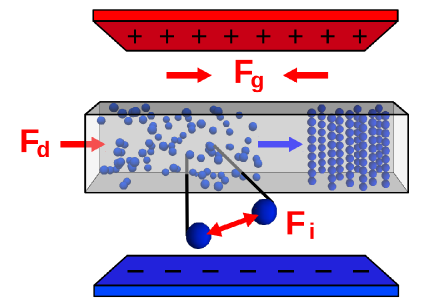
Figure 1: Formation of particle chains through the interaction of the drag force $F_{d}$ and magnetic forces. In the picture the magnetic forces are created by the magnetic field gradient $F_{g}$ and magnetic interactions $F_{i}$. The nonuniform magnetic field is created by 2 magnetic charge sheets.

Under the influence of the magnetic field a magnetic moment m is created in every particle. With the moments of two nearby beads and the distance r we got a formulation (Eqn. 1) of the interaction force $F_{i}$ for bead 2 and vice versa for bead 1 [5].

$$\vec{F}_{1\rightarrow 2}=\frac{3\mu_{0}}{4\pi r^{5}}[(\vec{m}_{1}\vec{r})\vec{m}_{2}+(\vec{m}_{2}\vec{r})\vec{m}_{1}+(\vec{m}_{1}\vec{m}_{2})\vec{r}-\frac{5(\vec{m}_{1}\vec{r})(\vec{m}_{2}\vec{r})}{r^{2}}\vec{r}$$ (1)

The gradient force $\vec{F}_{g}$ (Eqn. 2) on a bead is given by the negative gradient of the energy of the magnetic dipole moment $\vec{m}$ in the field $\vec{B}$.

$$\vec{F}_{g}=\nabla(\vec{m}\vec{B})$$ (2)

In three dimensions it is given by

$$\vec{F}_{g}=\begin{pmatrix}F_{x}\\ F_{y}\\ F_{z}\end{pmatrix}=\begin{pmatrix}m_{x}\partial xB_{x}+m_{y}\partial xB_{y}+m_{z}\partial xB_{z}\\ m_{x}\partial xB_{y}+m_{y}\partial yB_{y}+m_{z}\partial yB_{z}\\ m_{x}\partial xB_{z}+m_{y}\partial zB_{y}+m_{z}\partial zB_{z}\end{pmatrix}$$ (3)

We assume that in the x-y plane the external field is homogeneous due to the distance and size of the charge sheets. For the calculation of the gradient force only the z-field derived in y is important.

$$\vec{F}_{g}=\begin{pmatrix}0\\ m_{z}\partial yB_{z}\\ 0\end{pmatrix}$$ (4)

The blood flow creates a drag force [6] on the particles. At a low velocity of 460 $\mu m/s$ as used at most in CTC-chips [2], the flow is laminar. Turbulent flow would appear at Reynolds number (Eqn. 5) more than unity.

$$Re=\frac{2r\rho v}{\eta}$$ (5)

During laminar flow the Stokes Law (Eqn. 6) is used to calculate the force $F_{d}$ on an object in a fluid, with particle radius r, density $\rho$ and viscosity $\eta$ of the fluid and the relative velocity $v$ of the particle. Krishnamurthy et al. [7] show that Stokes drag is a good approximation for the force acting on the beads.

$$F_{d}=6\pi\eta rv$$ (6)

For the above mentioned calculations of the magnetic particle dynamics we decided to expand the open-source particle simulator Yade [8]. It provides for example gravity force and collision detection using various engines. Additionally we developed magnetic and fluidic engines. In the simulations we integrate the Newtons equation of motion for magnetic particles under the influence of the drag force of the fluid, the gradient force of the external magnetic field and the gradient force of the field created by the particles themselves.

For every particle in the pipe we calculate the magnetic field from the permanent magnets analytically [9]. We represent the 2 magnets by charge sheets as commonly done by magnetic simulation [10]. The simulation parameters are listed in table 1.

For blood cell dynamics we implemented a cellular engine in Yade. This will be explained in the next section.

Blood
velocity	$460\times 10^{-6}$ m/s
viscosity	0.015 Ns/$m^{2}$
density	1.055 g/$cm^{3}$
Particles
radius	$10^{-6}$ m
susceptibility	0.4
magnetic saturation	1 T
Geometry
magnetic charge sheets	10 x 10 mm
pipe	10 x 0.05 x 0.02 mm
distance pipe-sheet	2 mm
pole density sheets	1.6 T

Table 1: Simulation parameters

2.2 Blood cell dynamics

The red blood cell consists of a cytoskeleton covered with a double layer membrane [11]. It has a biconcave form in its native state with a diameter of around 8 $\mu m$, a surface of 135 $\mu m^{2}$ and a volume of 94 $\mu m^{3}$. The structure is built from 33000 hexagons which in reality would contain different proteins such as Spektrin and Aktin. In its loose state there is almost no interaction force between these proteins (Fig. 2a). If there is an external force acting on the cell the cytoskeleton expands and gets stretched (Fig. 2b). The membrane is an almost incompressible layer regarding the plane and shear stresses. Capillaries have a smaller diameter than the red blood cells, but because of their elastic properties they make their way using the form of a projectile.

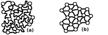
Figure 2: Cytoskeleton: a) relaxed, b) stretched

Discrete element methods can be used to treat red blood cells numerically. In the following we will show that the behavior of red blood cells can be modeled using a nonlinear mass-spring-system (Fig. 3). The model consists of nearly 600 spherical particles connected by springs arranged orthogonally.

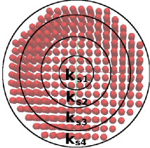
Figure 3: Nonlinear mass-spring model of red blood cell: $k_{s1}$=500, $k_{s2}$=400, $k_{s3}$=300, $k_{s4}$=200 (Eqn. 7)

The force between two particles i and j (Eqn. 7) depends on the respective spring constants, starting distance $l_{0}$ and the actual distance $d$. Yade provides the damping for all particles in the model.

$$F(x_{i},x_{j})=k_{s}*\frac{d}{|d|}*(|d|-l_{0})*|(|d|-l_{0})|$$ (7)

One possible way of characterizing a red blood cell is using an optical trap for extracting its shear modulus [12]. With an applied force on opposite sides of the cell, due to optical tweezers, the diameter is measured. From the approximated formula (Eqn. 8) the modulus decreases form the starting diameter $D_{0}$ with a function of the force F and the elasticity $\mu$.

$$D=D_{0}-\frac{F}{2\pi\mu}$$ (8)

To validate this model we computed this cell diameter as function of an applied stretch force (Fig. 4). Different spring constants are used to recreate a similar behavior in the stretching test. They decrease from the middle to the edge of the red blood cell (Fig. 3). The modeled cell is accurate enough to make tests with the chain barrier. This will be demonstrated in the result section.

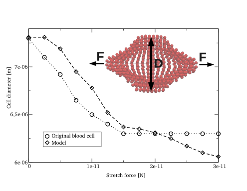
Figure 4: Stretch test of red blood cell, original [12] vs. model

3 Results

3.1 Single particle equilibrium position

With a steady blood flow through the microfluidic chip the magnetic particles are flushed out without the presence of an external magnetic field. To find the equilibrium position $y_{0}$ of a single bead after applying the field we calculate the force balance of the drag force $F_{d}$ and the gradient force $F_{g}$ (Eqn. 9). Fig. 6 shows this forces and their sum as function of the position. At the equilibrium state $F_{d}$ and $F_{g}$ cancel each other.

$$F_{g}(y)=F_{d}\quad\Longrightarrow\quad y_{0}$$ (9)

The magnetic moment $\vec{m}(y)$ of a single particle depends on its volume $V$, susceptibility $\chi$, which defines the ascending slope of the magnetization curve (Fig. 5), and the magnetic field. This field is the sum of the gradient field $B_{g}(y)$ and a homogenous bias field $B_{bias}$, which we will need to tune the device.

$$\vec{m}(y)=V\chi\frac{1}{\mu_{0}}(B_{g}(y)+B_{bias})$$ (10)

We have now 2 possible working points for the softmagnetic particles. In its saturated state (Fig. 5.1) the magnetic moment can’t be further increased. For better tunability we are using the working point in the initial magnetization curve (Fig. 5.2). This will be shown in the next sections.

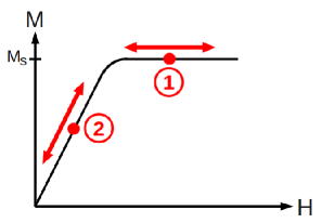
Figure 5: Operation points in the magnetization curve: 1. magnetic saturation, 2. initial magnetization (tunability)

The maximum field from the charge sheets is in the center and decreases towards the edge (Fig. 6). Fig. 7 shows the negative drag force and total magnetic force depending on the position of the magnetic particles. The results show that the final position depends on the strength of the uniform bias field and the susceptibility $\chi$ of the particles. If there is no crossing point the drag force is to high and the particles get washed out of the pipe (Fig. 7a with a bias field of less than $0.5T$).

If one of the simulation parameters changes, e.g. the viscosity of the blood, the drag force changes and therefore the external magnetic field has to change. Otherwise there probably wouldn’t be a crossing point, and therefore no equilibrium position.

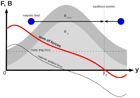
Figure 6: Magnetic charge sheets create a gradient field $B_{g}$. A homogenous bias field $B_{g}$ is added to the existing one for better tunability. Force balance of fluidic drag force $F_{d}$ and magnetic gradient force $F_{g}$ leading the particles to the equilibrium position $y_{0}$.

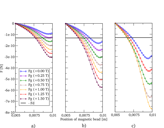
Figure 7: Gradient force $F_{g}$ as function of position with susceptibility a) 0.2 b) 0.4 c) 0.8. Crossing points with the drag force $F_{d}$ define the equilibrium position $y_{0}$ of a magnetic particle.

3.2 Chain formation

The simulation starts with softmagnetic beads of radius $1\mu m$ and susceptibility $0.4$. They are randomly located in the fluidic channel (Fig. 8a). Immediately after applying the magnetic charge sheets the particles self-organize to chains according to the field lines (Fig. 8b). This chain formation is then shifted to the equilibrium position $y_{0}$ because of the force balance explained in the section before. Because of chosen fluid velocity of 460 $\mu m/s$ this lasts around $16s$ (Fig. 8c).

After this procedure the filtering of the blood could start already. Different types of CTCs may need different distances between the chains for an optimal filtering. In the second phase of the simulation an additional homogenous bias field is applied on the chip. Depending on the field the chains change their gaps in around $0.13s$ (Fig. 8e). How it works will be explained in the next section.

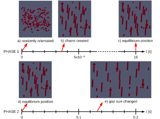
Figure 8: Timeline of the simulation: Phase 1 - Particle chain creation, Phase 2 - Changing the gap size

3.3 Tunable gap size

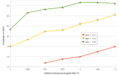
Figure 9: Average gap size between magnetic particle chains with different susceptibilities and additional external field

Eqn. 11 shows the magnetic moment $\vec{m}(y)$ of a single bead with the existance of many particles. When we increase the bias field $B_{bias}$ the magnetic moment and therefore the magnetic field created in every particle gets more. But only if we are in the working point of the initial magnetization curve (Fig. 5.2). The interaction field $B_{i}$ is the sum of all other particle fields. This leads to a higher particle interaction force which causes a larger gap.

Fig. 9 shows the increasing average gap size between the chains. In order to quantify this effect we computed the average distance between magnetic particle chains as a function of an additional homogenous magnetic field and susceptibility.

$$\vec{m}(y)=V\chi\frac{1}{\mu_{0}}(B_{g}(y)+B_{bias}+B_{i})$$ (11)

With a susceptibility of 0.2 resulting gaps occur only with an external field of more than $0.5T$. In this case the force caused by the fluid is greater than the maximum force of the gradient. So the particles get washed out of the pipe. At an intermediate susceptibility of 0.4 the gap size increases linearly with the field from $18\mu m$ to $24\mu m$. At high susceptibility the total field will saturate the particles which leads to similar results after $0.5T$.

3.4 Particle density

For the simulation result it is essential how dense the particles are filled into the pipe. For the particle density $\rho_{bead}$ we calculate the number of beads $N$ times the volume of one bead $V_{bead}$ over the volume of the wrapping box $V_{box}$ (Eqn. 12).

$$\rho_{bead}=\frac{N*V_{bead}}{V_{box}}$$ (12)

To evaluate the simulation we compared different starting densities and examined the resulting structures. Up to a density of 0.07 we find good results with not more than 2 bead thick chains. After that the particles get clumpy and can’t be used for our application. Fig. 10 demonstrates the different results of bead densities.

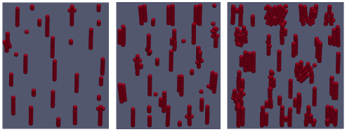
Figure 10: Endposition of chains with particle density 0.03, 0.07 and 0.11

3.5 Cell chain interaction

Very important for the functionality of the filter is the stability of the chains. When a blood cell touches such a chain a certain force is applied on it. And it would destroy the structure if it gets to high. To get a value of the force we started a simulation of our blood cell that flows directly on a particle chain that is fixed in space. Fig. 11 shows the average force per $ms$ over time acting from the blood cell to the chain, especially on one magnetic bead of the chain. The simulation overview is shown in Fig. 12. The magnitude of force on a single magnetic bead in the chain is 1000 times smaller than the drag force of the fluid or the gradient force of the magnetic charge sheets. So it doesn’t influence the position and the stability of the chain structure.

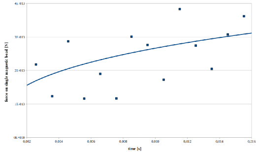
Figure 11: Force from the blood cell acting on a single magnetic bead of the chain structure.

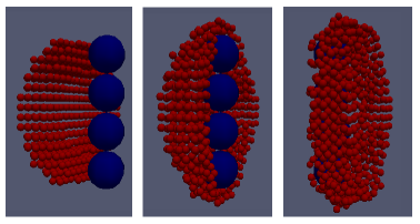
Figure 12: Red blood cell collides with a single magnetic chain for determing the contact force.

4 Summary

Flexible ways are important to get a high probability of catching cancer cells. Micromagnetic beads are established to create chain barriers on demand. Gap sizes are modified as desired for different CTCs. Size-based filtration and the usage of antibodies covered on the beads can take place simultaneously. In this work we demostrated simulation tools for the design of micromagnetic CTC-chips.

First step of modelling blood cells was the creation of a nonlinear mass-spring-system. For the success of the project it is essential to create models of all kind of blood cells, healthy ones and circulating tumor cells. More complex fluidic behavior is also important for future work. Turbulences could occur due to the selfarrangement of the chains in the magnetic field or the interaction of magnetic beads and blood cells.

Results summarized:

• Starting density of micromagnetic beads shouldn’t be more then 0.07 for the ratio between volume of beads and wrapping box.

• Softmagnetic beads self-organizes to particle chains due to the external aligned magnetic charge sheets within a few $\mu s$.

• After about 16s the chain arrangement finds its equilibrium position with the force balance of fluidic drag force and magnetic forces.

• Applying an additional homogenous field changes the gap size between the chains according to different circulating tumor cells in around $0.13s$.

• A nonlinear mass spring cell model in the flow creates a force on a magnetic bead in a chain with a magnitude of 1000 smaller than the drag force or the gradient force. So it has no influence on the chain structure.

Acknowledgment The authors gratefully acknowledge the financial support of Life Science Krems GmbH, the Research Association of Lower Austria.

References

- [1] B. Lu, T. Xu, S. Zheng, A. Goldkorn, Y. Tai, Parylene membrane slot filter for the capture, analysis and culture of viable circulating tumor cellsdoi:10.1109/MEMSYS.2010.5442361.
- [2] D. W. Bell, D. Irimia, L. Ulkus, M. R. Smith, E. L. Kwak, S. Digumarthy, A. Muzikansky, P. Ryan, U. J. Balis, R. G. Tompkins, D. A. Haber, M. Toner, S. Nagrath, L. V. Sequist, S. Maheswaran, Isolation of rare circulating tumour cells in cancer patients by microchip technology, Nature 450 (7173) (2007) 1235–1239. doi:10.1038/nature06385.
- [3] A. Saliba, L. Saias, E. Psychari, N. Minc, D. Simon, F. Bidard, C. Mathiot, J. Pierga, V. Fraisier, J. Salamero, V. Saada, F. Farace, P. Vielh, L. Malaquin, J. Viovy, Microfluidic sorting and multimodal typing of cancer cells in self-assembled magnetic arrays, Proceedings of the National Academy of Sciences 107 (33) (2010) 14524 –14529. doi:10.1073/pnas.1001515107.
- [4] P. J. Maimonis, K. Merdek, K. Dietenhofer, L. Yen, Y. Dong, G. Palmer, Affinity and size capture of circulating tumor cells: A platform for increased sensitivity, Proceedings of the American Association for Cancer Research 2010 (1_Molecular_Diagnostics_Meeting) (2010) B5.
- [5] E. P. Furlani, Permanent magnet and electromechanical devices: materials, analysis, and applications, Academic Press, 2001.
- [6] C. Mikkelsen, M. F. Hansen, H. Bruus, Theoretical comparison of magnetic and hydrodynamic interactions between magnetically tagged particles in microfluidic systems, Journal of Magnetism and Magnetic Materials 293 (1) (2005) 578–583. doi:10.1016/j.jmmm.2005.01.076.
- [7] S. Krishnamurthy, A. Yadav, P. E. Phelan, R. Calhoun, A. K. Vuppu, A. A. Garcia, M. A. Hayes, Dynamics of rotating paramagnetic particle chains simulated by particle dynamics, stokesian dynamics and lattice boltzmann methods, Microfluidics and Nanofluidics 5 (1) (2007) 33–41. doi:10.1007/s10404-007-0214-z.
- [8] J. Kozicki, F. Donzé, A new open-source software developed for numerical simulations using discrete modeling methods, Computer Methods in Applied Mechanics and Engineering 197 (49-50) (2008) 4429–4443. doi:10.1016/j.cma.2008.05.023.
- [9] G. Akoun, J. Yonnet, 3D analytical calculation of the forces exerted between two cuboidal magnets, IEEE Transactions on Magnetics 20 (5) (1984) 1962–1964. doi:10.1109/TMAG.1984.1063554.
- [10] K. Senanan, R. Victora, Theoretical study of nonlinear transition shift in double-layer perpendicular media, Magnetics, IEEE Transactions on 38 (4) (2002) 1664–1669. doi:10.1109/TMAG.2002.1017753.
- [11] A. Ikai, Einführung in die Nanobiomechanik: Bildgebung und Messung durch Rasterkraftmikroskopie, 1st Edition, Wiley-VCH Verlag GmbH & Co. KGaA, 2010.
-
[12]
S. Hénon, G. Lenormand, A. Richert, F. Gallet,
A
new determination of the shear modulus of the human erythrocyte membrane
using optical tweezers (Feb. 1999).
doi:16/S0006-3495(99)77279-6.
URL http://www.sciencedirect.com/science/article/pii/S0006349599772796