Characterization of the power excess of solar-like oscillations in red giants with Kepler

Abstract

Context. The space mission Kepler provides us with long and uninterrupted photometric time series of red giants. This allows us to examine their seismic global properties and to compare these with theoretical predictions.

Aims. We aim to describe the oscillation power excess observed in red giant oscillation spectra with global seismic parameters, and to investigate empirical scaling relations governing these parameters. From these scalings relations, we derive new physical properties of red giant oscillations.

Methods. Various different methods were compared in order to validate the processes and to derive reliable output values. For consistency, a single method was then used to determine scaling relations for the relevant global asteroseismic parameters: mean mode height, mean height of the background signal superimposed on the oscillation power excess, width of the power excess, bolometric amplitude of the radial modes and visibility of non-radial modes. A method for deriving oscillation amplitudes is proposed, which relies on the complete identification of the red giant oscillation spectrum.

Results. The comparison of the different methods has shown the important role of the way the background is modelled. The convergence reached by the collaborative work enables us to derive significant results concerning the oscillation power excess. We obtain several scaling relations, and identify the influence of the stellar mass and the evolutionary status. The effect of helium burning on the red giant interior structure is confirmed: it yields a strong mass-radius relation for clump stars. We find that none of the amplitude scaling relations motivated by physical considerations predict the observed mode amplitudes of red giant stars. In parallel, the degree-dependent mode visibility exhibits important variations. Both effects seem related to the significant influence of the high mode mass of non-radial mixed modes. A family of red giants with very weak dipole modes is identified, and its properties are analyzed.

Conclusions. The clear correlation between the power densities of the background signal and of the stellar oscillation induces important consequences to be considered for deriving a reliable theoretical relation of the mode amplitude. As a by-product of this work, we have verified that red giant asteroseismology delivers new insights for stellar and Galactic physics, given the evidence for mass loss at the tip of the red giant branch.

1 Introduction

The CNES CoRoT mission (Michel et al. 2006) and the NASA Kepler mission (Borucki et al. 2010) provide us with thousands of high-precision photometric light curves of red giants and have opened a new era in red giant asteroseismology (De Ridder et al. 2009). The asteroseismic analysis of these data gives a precise view of pressure modes (p modes), corresponding to oscillations propagating essentially in the large stellar convective envelopes, as well as of mixed modes, corresponding to pressure waves coupled to gravity waves propagating in the core radiative regions. Previous work has mainly dealt with the frequency properties of oscillations. In this paper, we explore and quantify the oscillation energy. This task is of prime importance for examining the link between convection and oscillations, including aspects such as mode excitation and damping. In parallel, examining the power density of the background signal will provide useful information on granulation.

The present work builds on previous studies based on CoRoT and Kepler observations, which derived first insights on the red giant oscillation spectrum and provided empirical scaling relations between the global seismic parameters (De Ridder et al. 2009; Hekker et al. 2009; Carrier et al. 2010; Bedding et al. 2010; Mosser et al. 2010; Huber et al. 2010; Mosser et al. 2011b). Very relevant to this work, Mathur et al. (2011) have determined the background signal due to the different time scales of activity and granulation, for the same set of Kepler red giants considered here. Additionally, Bedding et al. (2011) have recently shown with Kepler observations that the evolutionary status of red giant can be derived from the measurements of the gravity-mode spacing observable in $\ell=1$ mixed modes (Beck et al. 2011). With CoRoT data, Mosser et al. (2011a) have shown that the evolutionary status has also a clear effect on the oscillation power excess.

In this work, we provide a first complete description of the oscillation power excess and derive the bolometric amplitudes of radial modes. As in previous work, we establish scaling relations for global parameters as a function of frequency. Then, in order to provide a direct observational comparison to theoretical predictions (e.g. Dupret et al. 2009), scaling relations have to be established as a function of stellar parameters, such as luminosity (Christensen-Dalsgaard & Frandsen 1983; Kjeldsen & Bedding 1995; Houdek et al. 1999; Samadi et al. 2007). The influence of various parameters is tested, such as the evolutionary status and the stellar mass.

Data, methods and definitions are presented in Sect. 2 and in the Appendix. After the comparison of the different methods used for measuring the global energetic parameters, scaling relations are derived in Sect. 3. The fine structure of these relations is examined in Sect. 4. In Sect. 5, we propose a method for directly deriving the amplitudes of radial and non-radial modes, using the complete identification of the red giant oscillation spectra. This method is also used in Sect. 6 to compare observed bolometric amplitudes to available relationships, and in Sect. 7 to determine mode visibilities.

2 Data and method

2.1 Time series

The stars analyzed in this work have already been presented (Hekker et al. 2011a, and references therein). Their Kepler magnitudes are in the range 8 – 12.3, with most of them fainter than magnitude 11. They show oscillations in the frequency range [1, 280 $\mu$Hz], for which Kepler long-cadence data are well suited, having an average sample time of 1765.5 s, and so a Nyquist frequency of 283.5 $\mu$Hz. This work includes all available data, providing time series of about 590 days for more than a thousand red giants, giving a frequency resolution of about 19.7 nHz. The time series were prepared from the raw data (Jenkins et al. 2010) according to the method presented by García et al. (2011), which provides correction for various instrumental artefacts. The mean duty cycle is 91.5 %, with data loss mainly due to large but rare interruptions. In a few cases, 3-month long gaps occur for stars falling on the damaged CCD in the Kepler focal plane.

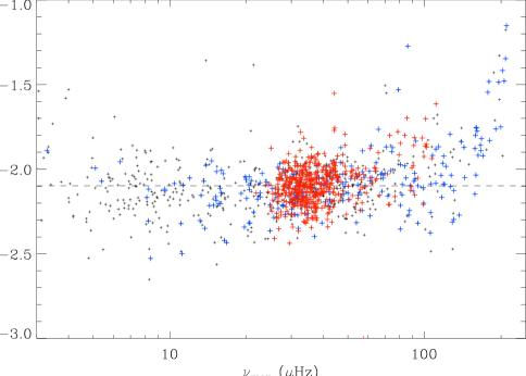
Figure 1: Local value of the exponent ${\alpha_{B}}$ of the background as derived from Eq. 3, as a function of $\nu_{\mathrm{max}}$. The dashed line indicates the median value estimated in the range [5, 120 $\mu$Hz]. The increase of ${\alpha_{B}}$ at large frequency is an artefact due to the Nyquist frequency. The color code indicates the evolutionary status: clump stars in red, red giant branch stars in blue, and undetermined status in black.

2.2 Background and power excess

To define the different components making up the signal, we used the classical phenomenological description of an oscillation power excess described by a mean Gaussian profile superimposed on the background (Michel et al. 2008). This means that the power density spectrum is composed of three components: the background $B$, which is assumed to be dominated by stellar noise at low frequency, the oscillation signal $P$ centered at $\nu_{\mathrm{max}}$, and white photon shot noise. The frequency $\nu_{\mathrm{max}}$ corresponds to the location of the maximum oscillation signal, according to the description of the Gaussian envelope:

$$P(\nu)={H}_{\nu_{\mathrm{max}}}\exp\left[-{(\nu-\nu_{\mathrm{max}})^{2}\over 2\sigma^{2}}\right],$$ (1)

where $\delta\nu_{\mathrm{env}}=2\sqrt{2\ln 2}\,\sigma$ is the full-width at half-maximum (FWHM) of the mode envelope, and ${H}_{\nu_{\mathrm{max}}}$ the height at $\nu_{\mathrm{max}}$. We note that, for the bright red giants considered here, the photon noise component is negligible compared to the other components.

In the global approach, the background $B$ is described by Harvey-like components. Each component is a modified Lorentzian (Harvey 1985):

$$B(\nu)=\sum_{i}{b_{i}\over 1+(2\pi\,\nu\tau_{i})^{\alpha_{i}}},$$ (2)

where $\tau_{i}$ is the characteristic time scales of the $i$-th component of maximum height $b_{i}$. The total number of components varies from 1 to 3 in the different methods. Such a model provides an accurate description of the background, although it is phenomenological. The introduction of a Lorentzian is linked to the assumption that the background signal is composed of independent components with an exponential decay in the time domain. In practice, the exponents $\alpha_{i}$, when fixed, are chosen to be close to 2 or 4.

Mathur et al. (2011) explicitly addressed this description of the red giant power spectra. Their work shows that the frequency $(2\pi\tau)^{-1}$ of the granulation component close to $\nu_{\mathrm{max}}$ is, in fact, closely correlated with $\nu_{\mathrm{max}}$; it varies as $\nu_{\mathrm{max}}^{0.89}$. In this work, we are mainly concerned with the value ${B}_{\nu_{\mathrm{max}}}$ of the background at $\nu_{\mathrm{max}}$. In that respect, a local description of $B(\nu)$ in the vicinity of $\nu_{\mathrm{max}}$ provides a model of sufficient precision. We have found that a polynomial approximation of the form

$$B(\nu)={B}_{\nu_{\mathrm{max}}}\left(\nu\over\nu_{\mathrm{max}}\right)^{\alpha_{B}}$$ (3)

is more precise than a linear fit. The expression holds in the frequency range $[\nu_{\mathrm{max}}-\delta\nu_{\mathrm{env}},\nu_{\mathrm{max}}+\delta\nu_{\mathrm{env}}]$. The local parameters were estimated in the frequency ranges surrounding the region where oscillation power excess is observed. The exponent ${\alpha_{B}}$ is found to be $-2.1\pm 0.3$ (Fig. 1). According to the relation between $1/\tau$ and $\nu_{\mathrm{max}}$ (Mathur et al. 2011), this supports an exponent close to 2 in the Harvey profile (Eq. 2), with a typical frequency $1/\tau$ smaller than $2\ \nu_{\mathrm{max}}$. If a modified expression including a term in $\nu^{4}$ is preferred to account for a rapid decrease of the background at higher frequency than $\nu_{\mathrm{max}}$, the measurement of ${\alpha_{B}}$ close to $-2$ implies stringent conditions between $\nu_{\mathrm{max}}$ and $1/\tau$. We conclude that, at lower frequencies, an exponent of 2 works reasonably well, whereas at higher frequencies a higher power of about 4 may be required to reproduce a steeper gradient, presumably reflecting smaller length scales in the turbulent cascade describing the convection.

The global description of the background (Eq. 2) is intended to be more accurate than the local description (Eq. 3). However, until we have a physical description of the background and its different scales, the global description remains phenomenological. We must keep in mind that crosstalk between the different components of the signal might add or remove energy from the oscillation signal. In that respect, testing the local description of the background, which is certainly not a correct solution, offers the possibility to fit the background with a minimum number of components.

In order to obtain the global parameters of the Gaussian envelope, most of the methods used for this work first consider a smoothed spectrum. The best practice for achieving this step is described in Appendix A and B.

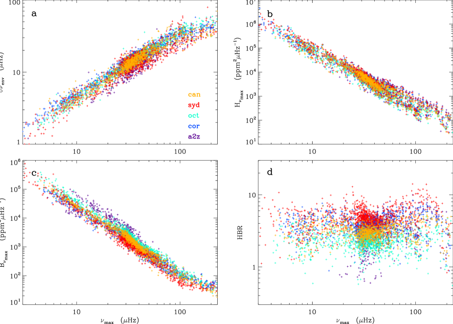
Figure 2: Global seismic parameters as a function of $\nu_{\mathrm{max}}$ derived from the five methods used here. a) FWHM $\delta\nu_{\mathrm{env}}$ of the Gaussian envelope; b) Mode height ${H}_{\nu_{\mathrm{max}}}$, as defined by Eq. 1, corrected for apodization; c) Background at $\nu_{\mathrm{max}}$. The increase above 200 $\mu$Hz is an artefact due to the proximity of the Nyquist frequency. d) Height-to-background ratio, affected by the artefact on ${B}_{\nu_{\mathrm{max}}}$. The color code indicates the method used for the data analysis, as indicated in panel a). The deviations from the trends above 200 $\mu$Hz are due to the proximity to the Nyquist frequency.

3 Scaling relations for global energy parameters

3.1 Comparison of the methods

We focus on the three global parameters previously introduced for describing the power excess (Eqs. 1-3):

• The FWHM $\delta\nu_{\mathrm{env}}$ of the Gaussian envelope, which measures the extent of efficient excitation of the oscillations. As we already know from CoRoT observations, the FWHM increases significantly with $\nu_{\mathrm{max}}$ (Fig. 2a). This envelope width is important to estimate the number $n_{\mathrm{env}}=\delta\nu_{\mathrm{env}}/\Delta\nu$ of radial orders with detectable amplitudes. This number can be compared to the order of maximum signal, defined as $n_{\mathrm{max}}=\nu_{\mathrm{max}}/\Delta\nu-\varepsilon(\Delta\nu)$.

• The oscillation height $H$ is measured at $\nu_{\mathrm{max}}$ (Fig. 2b).

• The background signal underlying the oscillation signal is taken as the height ${B}_{\nu_{\mathrm{max}}}$ at $\nu_{\mathrm{max}}$ (Fig. 2c). From ${B}_{\nu_{\mathrm{max}}}$, we can derive the height-to-background ratio ${H}_{\nu_{\mathrm{max}}}/{B}_{\nu_{\mathrm{max}}}$ (Fig. 2d).

The preliminary normalization process (Appendix A) ensures all methods produced results in global agreement. Small differences nevertheless remain, mostly being related to the way the background is modelled, particularly the number of components in the background profile. The differences have a stronger impact on the multiplicative coefficients than on the exponents of the scaling relations. Despite the correction of the time-domain averaging effect towards high frequencies due to the half-hour integration time, expressed by the suppression factor $\hbox{sinc\,}(\pi\nu_{\mathrm{max}}/2\nu_{\mathrm{Nyquist}})$, we note that all methods are affected by the Nyquist frequency. When $\nu_{\mathrm{max}}$ is close to $\nu_{\mathrm{Nyquist}}$, it becomes difficult to estimate the background, and unsurprisingly all methods tend to underestimate it since fewer modes are observable. As a result, the following analysis is limited to stars with $\nu_{\mathrm{max}}<200\,\mu$Hz.

The parameter showing the best agreement between the different methods is the envelope width $\delta\nu_{\mathrm{env}}$, while the parameter with the largest spread is the height-to-background ratio. This reflects systematic variations in the way the different components of the Fourier spectrum were fitted. We note systematic differences in ${H}_{\nu_{\mathrm{max}}}$ and ${B}_{\nu_{\mathrm{max}}}$, often with anticorrelated variations. We also note a change at the clump-frequency, which is certainly real, and is studied in detail in Sect. 4. Finally, we consider that the local description of the background provides results intermediate between the different global descriptions based on Harvey profiles. We therefore chose to use it for analyzing the scaling relations in the following sections.

Table 1: Comparison of global seismic parameters

method	$\Delta\nu$	$\delta\nu_{\mathrm{env}}$	${H}_{\nu_{\mathrm{max}}}/10^{7}$	${B}_{\nu_{\mathrm{max}}}/10^{6}$
A2Z	0.269;0.755	0.49;0.89	0.90;$-$2.10	11.1;$-$2.56
CAN	0.292;0.740	0.71;0.82	1.95;$-$2.35	5.75;$-$2.31
COR	0.286;0.744	0.74;0.84	1.69;$-$2.28	3.76;$-$2.23
OCT	0.271;0.756	0.57;0.90	1.74;$-$2.38	8.16;$-$2.37
SYD	0.283;0.747	0.63;0.85	1.95;$-$2.32	5.36;$-$2.39

- Each column gives a doublet $\alpha;\beta$, respectively coefficient and exponent of the power laws $\alpha\,\nu_{\mathrm{max}}^{\beta}$ of each parameter.

- Frequencies are all expressed in $\mu$Hz, and heights in ppm${}^{2}\mu$Hz^-1.

- The different methods provided results for a number of targets varying between 720 and 1220.

3.2 Scaling relations

Scaling relations for $\delta\nu_{\mathrm{env}}$, ${H}_{\nu_{\mathrm{max}}}$ and ${B}_{\nu_{\mathrm{max}}}$ as a function of $\nu_{\mathrm{max}}$ show clear global trends (Table 1, Fig. 2). Mean values of the coefficients and exponents of the best fits derived with all methods are given in Table 2. The dispersion with respect to the power laws, even if larger than for the $\nu_{\mathrm{max}}-\Delta\nu$ relation, are fairly small. Many reasons, with different origins, can explain this. Only physical reasons related to the seismic properties are discussed below. Other factors, such as the influence of unidentified close companions or background objects on the red giant light curves, are not relevant in this study since the red giants currently accessible were chosen to be bright and in uncrowded fields.

• The scaling relation for $\delta\nu_{\mathrm{env}}$ observed for CoRoT targets is confirmed. The ‘saturation’ above 200 $\mu$Hz is certainly related to the difficulty in estimating the background when $\nu_{\mathrm{max}}$ is close to $\nu_{\mathrm{Nyquist}}$. As stated earlier, stars with $\nu_{\mathrm{max}}$ greater than 200 $\mu$Hz were not considered in the following scaling relations. But we also note a saturation in the frequency range [100, 200 $\mu$Hz] that cannot be explained by this artefact. This effect is studied in detail in Sect. 4.

• The number of observable degrees varies as $\delta\nu_{\mathrm{env}}/\Delta\nu$. It decreases slowly at low frequency since it scales as $\nu_{\mathrm{max}}^{0.13}$ (Mosser et al. 2010).

• The stellar background signal varies as $\nu_{\mathrm{max}}^{-2.4}$. The exponent differs from the value $-2$ observed for subgiants and main-sequence stars (Chaplin et al. 2011).

• The exponents of the oscillation and background heights are approximately equal. As a consequence, the HBR appears to be constant with frequency (Fig. 2d). This was not the case in CoRoT data, where the background for many stars was dominated by the stellar photon noise, without a possibility to disentangle precisely the photon noise component from the stellar background. Here, photon noise is negligible compared to the stellar background for the majority of the targets. The HBR at $\nu_{\mathrm{max}}$ measures the energy density of the oscillations relative to the stellar background. The constant ratio, equal to about 3.8, is discussed in the next section. We note that the HBR values in Fig. 2d have a high dispersion in the frequency range [30, 60  $\mu$Hz]. The very large number of objects observed in this range excludes spurious variation due to a poor sampling: these stars definitely present characteristics that cannot be described by a single power law in $\nu_{\mathrm{max}}$.

For the remainder of the discussion, all results are based, for consistency, on a single method (COR, Table 5).

Table 2: Scaling relations

parameter	coefficient $\alpha$	exponent $\beta$
$\Delta\nu$	$0.276\pm 0.002$	$0.751\pm 0.002$
$n_{\mathrm{max}}=\nu_{\mathrm{max}}/\Delta\nu$	$3.52\pm 0.004$	$0.253\pm 0.002$
$\delta\nu_{\mathrm{env}}$	$0.66\pm 0.01$	$0.88\pm 0.01$
$n_{\mathrm{env}}=\delta\nu_{\mathrm{env}}/\Delta\nu$	$2.33\pm 0.01$	$0.13\pm 0.01$
${H}_{\nu_{\mathrm{max}}}$	$(2.03\pm 0.05)\;10^{7}$	$-2.38\pm 0.01$
${B}_{\nu_{\mathrm{max}}}$	$(6.37\pm 0.02)\;10^{6}$	$-2.41\pm 0.01$

- Mean values from the combined results of all methods.

- Each parameter is estimated as a power law of $\nu_{\mathrm{max}}$, namely varying as $\alpha\,\nu_{\mathrm{max}}^{\beta}$, with $\alpha$ the coefficient and $\beta$ the exponent.

- Frequencies are all expressed in $\mu$Hz, and heights in ppm${}^{2}/\mu$Hz.

- Scaling relations concerning $\delta\nu_{\mathrm{env}}$ are only valid for stars with $\nu_{\mathrm{max}}$ less than 100 $\mu$Hz.

4 Fine detail

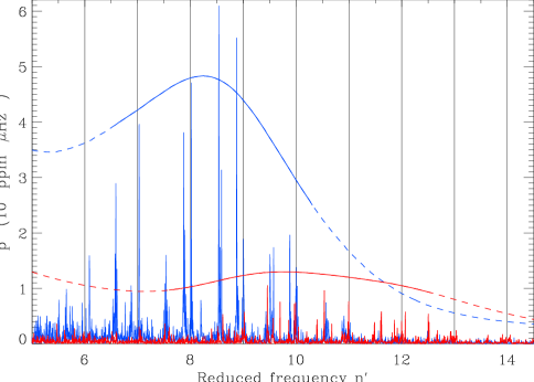
Figure 3: Comparison of two stars with similar large separations, one belonging to the RGB (KIC 4750456, $\Delta\nu=5.89\,\mu$Hz, blue curve) and the other to the secondary clump (KIC 3758458, $\Delta\nu=5.87\,\mu$Hz, red curve). The x-axis is the reduced frequency $n^{\prime}$; vertical lines indicate radial modes. The dashed curves represent 20 times the smoothed spectra; the regions corresponding to the FWHM are overplotted with solid lines.

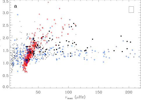
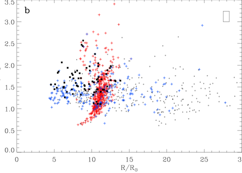
Figure 4: Asteroseismic mass as a function of $\nu_{\mathrm{max}}$ (panel a) and of the asteroseismic radius (panel b). The color code indicates the evolutionary status; clump stars in red, giant branch stars in blue, unknown status in dark grey. The population of giants with low $\ell=1$ amplitude (identified later in Sect. 7.1.1) is indicated with black squares. The rectangles in the upper right corners indicate the mean value of the 1-$\sigma$ error bars.

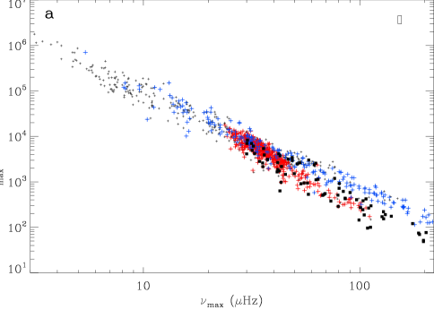
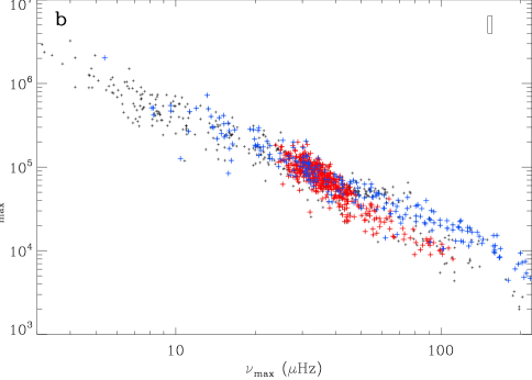
Figure 5: Maximum height ${H}_{\nu_{\mathrm{max}}}$ at $\nu_{\mathrm{max}}$ (panel a) and product ${H}_{\nu_{\mathrm{max}}}\delta\nu_{\mathrm{env}}$ (panel b), as a function of $\nu_{\mathrm{max}}$. Evolutionary status and mean error bars are indicated as in Fig. 4.

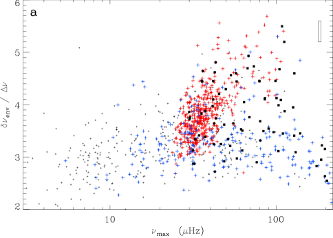
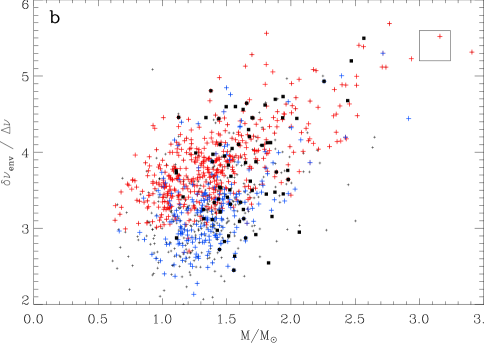
Figure 6: FWHM in unit $\Delta\nu$ as a function of $\nu_{\mathrm{max}}$ (panel a) and of the seismic mass (panel b). Evolutionary status and mean error bars are indicated as in Fig. 4.

Since we lack theoretical explanations for the observed scaling relations, we examine in this section how these relations are influenced by stellar parameters. The role of the stellar mass is potentially important since the mass distribution is degenerate with $\nu_{\mathrm{max}}$ (Mosser et al. 2010). So, we have derived an estimate of the asteroseismic mass from the scaling relations for $\Delta\nu$ and $\nu_{\mathrm{max}}$ to address this mass influence.

In a next step, we have examined whether the relations discussed in Sect. 3 vary with the evolutionary status. The direct comparison of two stars with similar large separations but different evolutionary status, one belonging to the red giant branch and the other to the red clump, clearly shows that the clump stars present much lower amplitudes, but larger values of $\nu_{\mathrm{max}}$ and $\delta\nu_{\mathrm{env}}$, hence a higher acoustic cutoff frequency (Fig. 3). The relation between $\nu_{\mathrm{max}}$ and the cutoff frequency has been shown observationally, and is now assessed theoretically (Belkacem et al. 2011).

4.1 Mass-radius relation

In order to investigate how global seismic parameters vary with both mass and evolutionary status, we must illustrate how the mass, radius and evolutionary status are linked. Fig. 4 shows how the stellar masses and radii are distributed with $\nu_{\mathrm{max}}$ and how they are correlated with the evolutionary status. For stars on the red giant branch (RGB), the mass distribution is nearly uniform across the whole frequency range. On the other hand, the distribution of $\nu_{\mathrm{max}}$ and mass are clearly correlated for clump stars, as already shown with CoRoT data. The same features are clearly found in the mass-radius relation, since stellar radius and $\nu_{\mathrm{max}}$ are strongly correlated. A discussion in terms of stellar evolution, mass loss, and reset of the red giant structure at the helium flash for low-mass stars, has already been presented by Mosser et al. (2011a). Here, the clear difference between RGB and clump stars helps to identify the structure present in Fig. 2b: the apparent slope change in the ${H}_{\nu_{\mathrm{max}}}$ and ${B}_{\nu_{\mathrm{max}}}$ relations is linked to the highly non-uniform mass distribution for $\nu_{\mathrm{max}}$ in the frequency range [30, 60 $\mu$Hz] due to clump stars.

4.2 Power excess, mass, and evolutionary status

We have revisited the scaling relations dealing with the power excess according to the evolutionary status of the red giants (Figs. 5 and 6). This reveals a clear difference between the two populations.

• For stars with $\nu_{\mathrm{max}}$ in the range [25-50 $\mu$Hz]: red clump stars and RGB stars have similar masses, but the distribution of the mass on the RGB is not correlated with $\nu_{\mathrm{max}}$, whereas there is a clear correlation for red-clump stars (Fig. 4). At the same time, the global energy parameters are similar for both populations, but with somewhat different slopes (Fig. 5).

• At higher $\nu_{\mathrm{max}}$ we find the secondary clump, consisting of He-burning stars of higher masses (Girardi 1999). With increasing mass, the maximum mode height of secondary clump stars decreases significantly. In parallel, the FWHM of the Gaussian envelope increases. In stars burning helium in their core, the energy partition differs significantly: a wider range of modes is excited but with much lower oscillation heights. This can be understood when recalling the link between $\nu_{\mathrm{max}}$ and the cutoff frequency $\nu_{\mathrm{c}}$ (Kjeldsen & Bedding 1995; Belkacem et al. 2011). At fixed $\Delta\nu$ (as for the two red giants shown in Fig. 3), a low-mass star has a much lower $\nu_{\mathrm{max}}$ than a member of the secondary clump. The explicit mass dependence of the FWHM $\delta\nu_{\mathrm{env}}$ is shown in Fig. 6. The product ${{H}_{\nu_{\mathrm{max}}}\delta\nu_{\mathrm{env}}}$ (Fig. 5b) tells us that oscillations in clump stars have less energy than in the RGB.

• The saturation of $\delta\nu_{\mathrm{env}}$ observed in the frequency range [100 - 200 $\mu$Hz] only concerns RGB stars. It occurs at too low a frequency to be related to the Nyquist frequency, and clearly departs from the scaling relation reported in Table 1. We have to conclude that the mechanism of excitation is only efficient in a limited frequency range. This may be due to a change in the relation between $\nu_{\mathrm{max}}$ and the atmospheric cutoff frequency (Belkacem et al. 2011). Finally, we can derive a relation between $\delta\nu_{\mathrm{env}}$ and the stellar mass, expressed by the number of observable radial orders:

$$n_{\mathrm{env}}\equiv{\delta\nu_{\mathrm{env}}\over\Delta\nu}=\left\{\begin{array}[]{rrl}2.72&+\ 0.87\ M/M_{\odot}&\qquad\hbox{(clump)}\\ 2.37&+\ 0.77\ M/M_{\odot}&\qquad\hbox{(RGB)}\\ \end{array}\right.$$ (4)

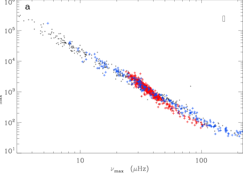
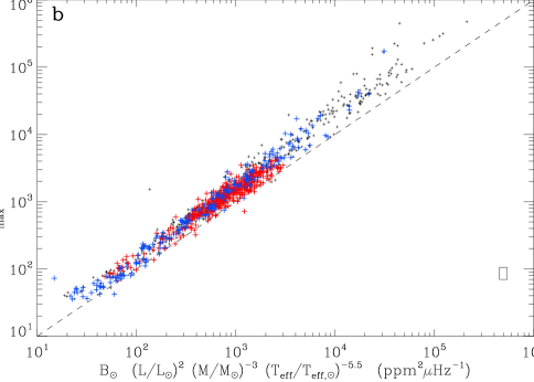
Figure 7: Background ${B}_{\nu_{\mathrm{max}}}$ as a function of $\nu_{\mathrm{max}}$ (panel a), and as a function of $B_{\odot}\,\Lambda_{\mathrm{B}}$ (panel b), with the solar value $B_{\odot}=0.19$ ppm${}^{2}\,\mu$Hz^-1. Evolutionary status and error bars are indicated as in Fig. 4. The dashed line indicates the 1:1 relation.

4.3 Granulation background

We have tested the new relation giving ${B}_{\nu_{\mathrm{max}}}$ as a function of $\Lambda_{\mathrm{B}}=(L/L_{\odot})^{2}(M/M_{\odot})^{-3}(T_{\mathrm{eff}}/T_{\odot})^{-5.5}$ (Kjeldsen & Bedding 2011). We made use of the asteroseismic estimate of the luminosity derived from the asteroseismic radius, the effective temperature (Brown et al. 2011) and the Boltzmann law. Such luminosity values certainly suffer from scaling uncertainties. This means that the absolute values are less reliable than relative variations. In other words, the exponent of the relation predicting ${B}_{\nu_{\mathrm{max}}}$ is less biased than the multiplicative coefficient.

The function ${B}_{\nu_{\mathrm{max}}}(\nu_{\mathrm{max}})$ shows two different branches with different slopes (Fig. 7a), whereas ${B}_{\nu_{\mathrm{max}}}(\Lambda_{\mathrm{B}})$ seems to be able to reconcile both evolutionary states (Fig. 7b). The phenomenological expectation seems verified, since the exponent is not far from unity, in agreement with Huber et al. (2011):

$${B}_{\nu_{\mathrm{max}}}=\left\{\begin{array}[]{rll}0.16&\Lambda_{\mathrm{B}}^{1.08}&\qquad\hbox{(all)}\\ 0.28&\Lambda_{\mathrm{B}}^{1.01}&\qquad\hbox{(clump)}\\ 0.15&\Lambda_{\mathrm{B}}^{1.09}&\qquad\hbox{(RGB)}\\ \end{array}\right.$$ (5)

We note that the coefficient of the fit of all red giants is very close to the value of the solar background at $\nu_{\mathrm{max}}$ of about 0.19 ppm${}^{2}\,\mu$Hz^-1 found by Huber et al. (2011). This value has been used in Fig. 7b. We see that the relation predicts too low values of the background at $\nu_{\mathrm{max}}$.

Having previously remarked that the HBR has a uniform value across a wide frequency range, we have then to examine whether ${H}_{\nu_{\mathrm{max}}}$ also scales with $\Lambda_{\mathrm{B}}$. This is the case, with exponents close to 1 for both RGB and clump stars, but with a different ratio. We measure:

$${{H}_{\nu_{\mathrm{max}}}\over{B}_{\nu_{\mathrm{max}}}}=\left\{\begin{array}[]{cl}3.67\pm 0.07&\qquad\hbox{(clump)}\\ 4.02\pm 0.12&\qquad\hbox{(RGB)}\\ \end{array}\right.$$ (6)

Kjeldsen & Bedding (2011) postulated that the mean height of modes, observed in velocity, is proportional to the velocity power density of the granulation at $\nu_{\mathrm{max}}$. Here, we show that this proportionality is verified in the photometric signal for red giants. A similar study for all stellar classes was made by Huber et al. (2011), who reached similar conclusions.

5 Amplitudes

It has been suggested that oscillation amplitudes depend on the luminosity-to-mass ratio (Christensen-Dalsgaard & Frandsen 1983; Kjeldsen & Bedding 1995; Houdek et al. 1999; Samadi et al. 2007). They also depend on the mode degree. As we found a large diversity in the red giant oscillation spectra, we propose in this section a method for measuring separately the radial and non-radial amplitudes in red giants facilited by the automated mode identification provided by the red giant universal oscillation pattern (Appendix C). The measurements will then allow us to derive bolometric amplitudes and also mode visibilities, in Sect. 6 and 7 respectively.

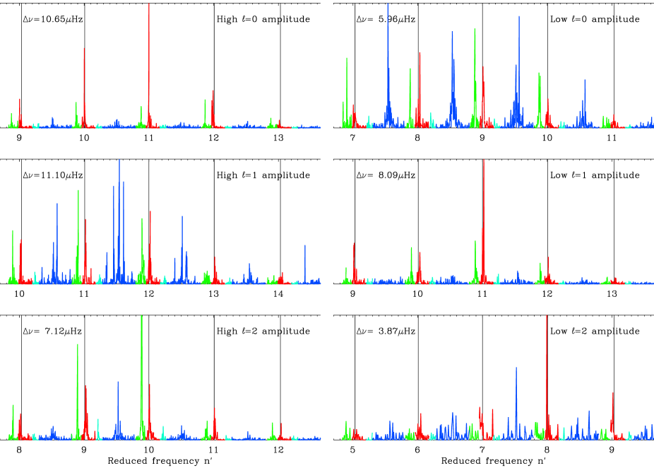
Figure 8: Identification of the ridges in red giants observed by Kepler. Targets were chosen with oscillation spectra exhibiting very different visibility coefficients (see Sect. 7). Left side: high visibility of $\ell$=0 to 2 from top to bottom. Right side: low visibility of $\ell$=0 to 2 from top to bottom. The spectra are corrected for the background contribution (negative values being omitted), and plotted as a function of the reduced frequency. The color code, derived from Eqs. 7 and 8, presents radial modes in red, $\ell=1$ in blue, $\ell=2$ in green, and $\ell=3$ in light blue.

5.1 Radial amplitudes

Previously, the amplitudes of radial modes have been derived from the mean amplitude in the oscillation envelope divided by the total visibility factors of the modes (Kjeldsen et al. 2008; Michel et al. 2009). Here, we have computed spectra as a function of the reduced frequency $n^{\prime}$ (Eq. 17). Squared amplitudes are then given by integrating the height across the mode width, as estimated from the fit of the ridges, with the integral being corrected for the background contribution. That is, we have computed the squared amplitudes for each radial order from:

$$A_{0}^{2}(n)=\delta\nu\ \int_{n-e_{20}}^{n+e_{03}}\bigl{[}p(n^{\prime})-B\bigr{]}\ \mathrm{d}n^{\prime}\$$ (7)

with $p$ the power density spectrum, $\delta\nu$ the frequency resolution, and $B$ the local background. The boundaries $e_{20}$ and $e_{03}$ bracket the frequency range where radial modes are expected: the radial mode $(n,0)$ lies between the $(n-1,2)$ and $(n-1,3)$ modes. They have been defined according to the parametrization proposed by Mosser et al. (2011b). We have checked that the measures of the radial amplitudes are stable with respect to slight modifications of these boundaries. The major contribution to the uncertainties comes from uncertainty on the background correction, resulting in a mean precision of about 10 %.

5.2 Non-radial amplitudes

Non-radial amplitudes have been calculated in the same way, with the appropriate boundaries $e_{\ell\ell^{\prime}}$ between the adjacent degrees $\ell$ and $\ell^{\prime}$:

$$A_{\ell}^{2}(n)=\delta\nu\ \int_{n-e_{\ell^{\prime}\ell}}^{n+e_{\ell\ell^{\prime\prime}}}\bigl{[}p(n^{\prime})-B\bigr{]}\ \mathrm{d}n^{\prime}\ .$$ (8)

We have used the mean values $e_{12}=-0.22$, $e_{20}=-0.065$, $e_{03}=0.17$, and $e_{31}=0.27$ derived from the universal red giant oscillation pattern (Mosser et al. 2011b). These boundaries are globally shifted by $0.008\,(n-n_{\mathrm{max}})$ to account for the mean curvature of the spectra, and modulated in large separation according to the exact location of the ridges (Table 1 of Mosser et al. 2011b). In case of mixed modes, the amplitude of a certain degree we measure corresponds to the sum of all individual components of a given pressure radial order $n$. A few examples are given in Fig. 8.

From the definition given by Eq. 8, it is clear that, in case of rotational multiplets, the method integrates the squared amplitudes of all components. In other words, the method is not affected by the unknown stellar inclination.

5.3 Mean values of individual amplitudes

The mean value of the individual amplitudes has been obtained under the assumption that the energy partition is Gaussian, following Eq. 1:

$$\langle A_{\ell}^{2}\rangle=\displaystyle{\sum_{n_{\mathrm{max}}-2}^{n_{\mathrm{max}}+2}A_{\ell}^{2}(n)}\ \Big{/}\ \displaystyle{\sum_{n_{\mathrm{max}}-2}^{n_{\mathrm{max}}+2}\exp\left[-{(\nu_{n,\ell}-\nu_{\mathrm{max}})^{2}\over 2\sigma^{2}}\right]}.$$ (9)

Formally, one would expect the weighting to be performed before the summation, but such a method is too sensitive to the varying amplitudes created by the stochastic excitation. Therefore, with Eq. 9, we intend to estimate a mean value not affected by this source of noise. Considering five radial orders is in agreement with the observed width of the envelope and allows us to pick the highest peaks.

5.4 Individual and globally averaged radial amplitudes

The radial amplitude has also been directly determined, by

$$A_{0}=A_{0}(n_{\mathrm{max}}).$$ (10)

We have compared $\langle A_{0}^{2}\rangle^{1/2}$ to the radial amplitude $A_{0}$, and shown that both amplitudes are closely linked, with $A_{0}\simeq 1.07\ \langle A_{0}^{2}\rangle^{1/2}$. However, to avoid scattering due to the finite mode lifetimes and for coherence of the visibility calculation, we have decided to consider the radial amplitude $\langle A_{0}^{2}\rangle^{1/2}$. This value can be compared to the non-radial amplitudes in order to compute the mode visibilities. It can also be compared to the global average amplitudes derived from the total mode visibility (Kjeldsen et al. 2008; Michel et al. 2009)

$$\langle A\rangle=\sqrt{{H}_{\nu_{\mathrm{max}}}\Delta\nu\over V^{2}_{\mathrm{tot}}}.$$ (11)

The examination of the total mode visibility $V^{2}_{\mathrm{tot}}$ in Sect. 7 allows to compare $\langle A\rangle$ and $\langle A_{0}^{2}\rangle^{1/2}$ in more detail.

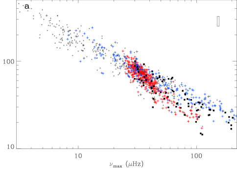
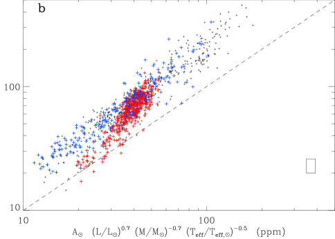
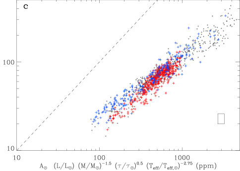
Figure 9: Bolometric amplitude $\mathcal{A}_{\mathrm{bol}}$, in ppm, as a function of $\nu_{\mathrm{max}}$ (panel a), $A_{\odot}\,(LM_{\odot}/L_{\odot}M)^{0.7}(T_{\mathrm{eff}}/T_{\odot})^{-0.5}$ (panel b) and $A_{\odot}\,(L/L_{\odot})(M/M_{\odot})^{-1.5}(\tau/\tau_{\odot})^{0.5}(T_{\mathrm{eff}}/T_{\odot})^{-2.75}$ (panel c), with the solar value $A_{\odot}\simeq 2.53$ ppm. Evolutionary status and error bars are indicated as in Fig. 4. The dashed lines show the 1:1 correspondence.

6 Bolometric amplitudes of radial modes

We now use the bolometric correction performed for Kepler observations by Ballot et al. (2011) to translate the observed radial amplitudes to bolometric amplitudes. We then examine how the bolometric radial amplitudes scale with various parameters and test the available theoretical amplitude scaling relations.

6.1 Bolometric correction

The bolometric correction provided by Ballot et al. (2011) allows us to derive bolometric amplitudes from the radial amplitudes:

$$\mathcal{A}_{\mathrm{bol}}=\langle A_{0}^{2}\rangle^{1/2}\ \mathcal{C}_{\mathrm{bol}}\hbox{ \ with \ }\mathcal{C}_{\mathrm{bol}}=(T_{\mathrm{eff}}/T_{K})^{0.80}$$ (12)

with $T_{K}=5\,934$ K. This correction accounts for the wavelength dependence of the photometric variation integrated over the Kepler bandpass. The variation of $\mathcal{A}_{\mathrm{bol}}$ with $\nu_{\mathrm{max}}$ shows clearly the differences between RGB and clump stars (Fig. 9a). We note that the difference is much more pronounced for the secondary clump, which contains objects with higher mass than the primary clump.

6.2 Comparison with $(L/M)^{0.7}$

We have compared these amplitudes to different relations depending on the stellar luminosity and mass. As in Sect. 4, both $L$ and $M$ were derived from the usual asteroseismic scalings relations. As discussed above, such scalings avoid the use of grid modelling, which only works at fixed physics, but certainly lower the quantitative validity of the outputs since the scaling relations are not yet accurately calibrated.

We have tested the variation in $(L/M)^{0.7}$ proposed by Samadi et al. (2007) for Doppler measurements, and verified that the observed exponent is effectively near the value 0.7 derived from 3-D simulations. As already shown by Mosser et al. (2010) and Huber et al. (2010), we find a slightly higher exponent, of about 0.8 (Fig. 9b and Table 3). We have introduced the correction from Doppler to photometric measures, expressed by a factor $\sqrt{T_{\mathrm{eff}}}$, under the assumption that the oscillations propagate adiabatically (Kjeldsen & Bedding 1995). We also adopted in the scaling relation the bolometric amplitude $A_{\odot}\simeq 2.53$ ppm of solar radial modes observed in broad-band photometry (Michel et al. 2009). We note that the relation underestimates the amplitude by a factor of about 2, and that the exponents are different for the different evolutionary states (Fig. 9b).

The theoretical relation proposed by Samadi et al. (2007) was derived for main-sequence stars, and applying it to red giants is a large extrapolation. Indeed, investigating mode driving in red giants would require a non-adiabatic treatment. From the oscillation energy equation (e.g. Unno et al. 1989, Chap. IV, Eq. 21.14), dimensional arguments show that non-adiabatic effects scale as the ratio $L/M$, which is roughly 50 times greater for red giants than for main-sequence stars. We might therefore expect the physics underlying mode driving to be different for the two cases. In principle, non-adiabatic effects must also be considered when converting between velocity amplitudes (as provided by theoretical computations) and photometric amplitudes (as measured with Kepler). However, in the absence of a reliable non-adiabatic theory, we have to adopt the adiabatic conversion (e.g. Kjeldsen & Bedding 1995; Samadi et al. 2010). These points deserve thorough theoretical investigation, but this is beyond the scope of this paper.

6.3 Comparison with $L/M^{1.5}$

We also tested the revised amplitude scaling relation suggested by Kjeldsen & Bedding (2011). It includes not only the mass and luminosity, but also the effective temperature and the mode lifetimes $\tau$:

$$\mathcal{A}_{\mathrm{bol}}\propto{\Lambda_{\mathrm{A}}}\hbox{ \ with \ }{\Lambda_{\mathrm{A}}}={(L/L_{\odot})\ (\tau/\tau_{\odot})^{0.5}\over(M/M_{\odot})^{1.5}\ (T_{\mathrm{eff}}/T_{\odot})^{2.75}}.$$ (13)

Baudin et al. (2011a) explored the observed mode lifetime for CoRoT data. They suggested that for red giants, $\tau$ is about 30 days and varies as $T_{\mathrm{eff}}^{-0.3\pm 0.8}$. We use these estimates here. When expressed as a function of $\Lambda_{\mathrm{A}}$, the two branches corresponding to RGB and clump stars show a closer correlation (Fig. 9c), so that the distribution of $\mathcal{A}_{\mathrm{bol}}$ as a function of $\Lambda_{\mathrm{A}}$ is less dispersed than the distribution as a function of $(L/M)^{0.7}$. However, the best fit gives a variation $\mathcal{A}_{\mathrm{bol}}\propto\Lambda_{\mathrm{A}}^{0.71\pm 0.02}$ instead of $\mathcal{A}_{\mathrm{bol}}\propto\Lambda_{\mathrm{A}}$ proposed by Kjeldsen & Bedding (2011). As a consequence, this theoretical relation largely overestimates the observed bolometric radial amplitudes, as also shown by Huber et al. (2011) and Stello et al. (2011). This means that the proposed relation does not provide a complete physical explanation. We also note that the prediction of $\mathcal{A}_{\mathrm{bol}}$ proportional to $L$ is observationally unlikely. For red giants, $L$ is the most rapidly varying parameter in Eq. 13, so that the observed slope in Fig. 9b almost directly translates into the luminosity exponent. The agreement between observed and predicted values would require $\tau$ to be approximately proportional to $\Delta\nu$, which is clearly not observed (Huber et al. 2010; Baudin et al. 2011a).

Despite the quantitative disagreement with theoretical predictions, we see from Figs. 9b and c that an empirical scaling relation can describe the variation of $\mathcal{A}_{\mathrm{bol}}$ as a function of the stellar luminosity, mass and effective temperature. Such a fit based on red giants in open clusters, hence with an accurate mass estimation, was proposed by Stello et al. (2011), which agrees with a fit based on red giants, subgiants and main-sequence stars performed by Huber et al. (2011).

Table 3: Bolometric amplitudes

scaling with		coefficient	exponent
$\nu_{\mathrm{max}}$	all	$860\pm 30$	$-0.71\pm 0.01$
	clump	$4700\pm 500$	$-1.18\pm 0.03$
	RGB	$650\pm 60$	$-0.63\pm 0.02$
$L/M$	all	$3.5\pm 0.2$	$0.79\pm 0.01$
	clump	$0.92\pm 0.11$	$1.12\pm 0.04$
	RGB	$4.8\pm 0.4$	$0.71\pm 0.02$
$\Lambda_{\mathrm{A}}$	all	$8.2\pm 0.2$	$0.70\pm 0.01$
	clump	$5.3\pm 0.3$	$0.83\pm 0.02$
	RGB	$9.8\pm 0.4$	$0.65\pm 0.02$

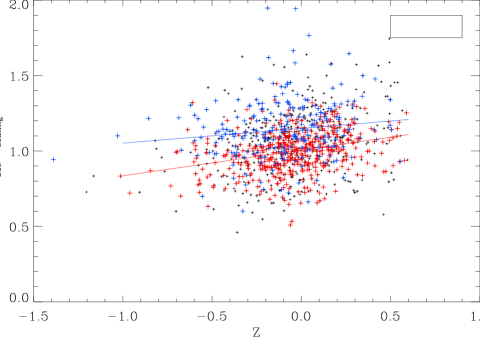
Figure 10: Variation in metallicity of the bolometric amplitude scaled to a best fit in $L/M^{1.5}$. Same color code as in Fig. 4. The red and blue lines corresponds to the linear fits in $Z$. The uncertainties on $Z$ are obtained from Brown et al. (2011).

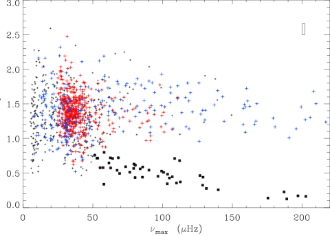
Figure 11: Visibility $V^{2}_{1}$ as a function of $\nu_{\mathrm{max}}$, with the same color code as in Fig. 4. Large black symbols indicate the population of stars with very low $V^{2}_{1}$ values.

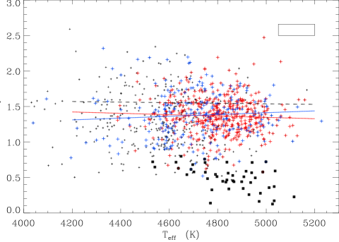
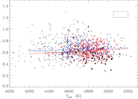
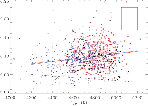
Figure 12: Visibility of the $\ell=1$, 2 and 3 modes (from top to bottom), as a function of the effective temperature. Same color code as in Fig. 11. Dashed lines are the fits derived from Ballot et al. (2011). Blue and red solid lines are the fits for RGB and clump stars, respectively.

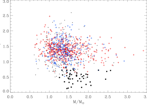
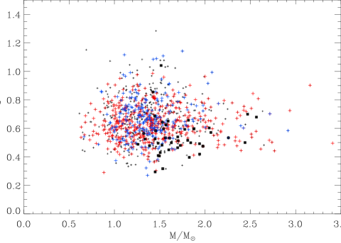
Figure 13: Visibility of the $\ell=1$ and 2 modes, as a function of the seismic mass. Same color code as in Fig. 11.

6.4 Influence of metallicity

It has been suggested that oscillation amplitudes depend on the stellar metallicity (Houdek et al. 1999; Samadi et al. 2010). In order to test this dependence, we have plotted the bolometric amplitudes as a function of the metallicity (Fig. 10). This comparison requires normalized amplitudes, which were obtained using a fit in $L/M^{1.5}$ (Huber et al. 2011). The metallicity values were taken from the Kepler Input Catalog (Brown et al. 2011) and have uncertainties of about 0.4 dex. We found that an increase of 1 dex in $Z$ gives a moderate amplitude increase of about 10$\pm$5 %. Further work, based on improved values of the metallicity, will be necessary to make the link more precise.

7 Spatial response functions

We have examined the visibility of each degree, obtained from

$$V^{2}_{\ell}=\langle A^{2}_{\ell}\rangle\ /\ \langle A^{2}_{0}\rangle,$$ (14)

with $\langle A^{2}_{0}\rangle$ given by Eqs. 7 and 9, and $\langle A^{2}_{\ell}\rangle$ obtained in a similar way. For pure p modes in a 4800 K red giant, one expects spatial response functions in power to vary as $V^{2}_{1}\simeq 1.54$, $V^{2}_{2}\simeq 0.58$ and $V^{2}_{3}\simeq 0.043$. These values, derived from Ballot et al. (2011), assume energy equipartition between the different degrees and take into account the influence of the limb darkening. They are expected to decrease when the effective temperature increases (Table 4). Fig. 8 shows the background-corrected spectra of different red giants exhibiting different mode visibilities.

7.1 Dipole modes

The visibilities $V^{2}_{1}$ of the dipole modes are plotted in Fig. 11 as a function of $\nu_{\mathrm{max}}$ and in Fig. 12a as a function of the effective temperature. We first note a large dispersion of the values and a discrepancy between observed and predicted values. In general, the observed $V^{2}_{1}$ appear to be smaller than expected. Despite including the mixed modes in a very broad frequency range, in fact larger than $\Delta\nu/2$, we observed $\langle V^{2}_{1}\rangle=1.34\pm 0.02$ instead of the expected value of 1.54 (Table 4). Individual uncertainties on $V^{2}_{1}$ are about $\pm 0.08$. They are principally due to the background modelling and to the difficulty of automatically identifying all mixed modes.

7.1.1 Very weak $V^{2}_{1}$ values

We note the presence of a family of stars with a very weak, almost absent $\ell=1$ oscillation pattern. It mostly comprises less evolved stars, with $\nu_{\mathrm{max}}\geq 50\,\mu$Hz and $V^{2}_{1}\leq 0.8$, which appear clearly as outliers. As a consequence of the low $\ell=1$ amplitudes, their evolution status is not determined, except for four stars, two in the RGB and two in the clump. Very low $V^{2}_{1}$ values are also measured at the clump, but without the clear difference compared to other stars. Therefore, we do not include them among the set of stars with very weak $V^{2}_{1}$ values. We limit it to $\nu_{\mathrm{max}}\geq 50\,\mu$Hz and a low $V^{2}_{1}$ (about $12.5\;\nu_{\mathrm{max}}^{-0.72}$, with $\nu_{\mathrm{max}}$ in $\mu$Hz).

Different tests have shown that, apart from a low $\ell=1$ visibility, these stars mostly share the common characteristics of other stars. Unsurprisingly, they have lower heights than expected from the empirical scaling relation since $\ell=1$ modes are almost absent, but their bolometric amplitudes are close to the mean values. More precisely, if one believes that the location in the $\mathcal{A}_{\mathrm{bol}}(\nu_{\mathrm{max}})$ relation (Fig. 9) makes it possible to identify the evolutionary status, clump stars with a low $V^{2}_{1}$ show normal bolometric amplitudes, but RGB stars with a low $V^{2}_{1}$ have lower amplitudes than expected. This could be related to the fact that these stars have slightly higher masses compared to the mean values (Fig. 13a). However, some stars do present simultaneously a high asteroseismic mass and a normal $V^{2}_{1}$. Their $\ell=2$ visibilities are slightly lower than average, but not significantly so. Furthermore, these stars are uniformly distributed in temperature and metallicity. Therefore, we have to conclude that only $\ell=1$ modes are affected. One may imagine that their suppression results from a very efficient coupling between pressure and gravity waves. This efficient coupling yields a very high mode mass, hence a very low observed amplitude at the surface. Examining the causes of very low $V^{2}_{1}$ values will need further work. It may also help to understand the non-identification of $\ell=1$ modes in previous observations of high-mass giants (Frandsen et al. 2002; Baudin et al. 2011b).

7.1.2 A surprising energy equipartition

Having identified the population with abnormally low $V^{2}_{1}$ values allows us to calculate the mean $\ell=1$ visibility of ‘normal’ red giants: it remains lower than the expected value (1.38, versus 1.54), and uncertainties are unable to explain the discrepancy. We note that the lower-than-expected $V^{2}_{1}$ values are independent of $\nu_{\mathrm{max}}$, hence independent of the evolution. Coming back to the way the amplitudes were determined, we see that the sum of the squared amplitudes of all $\ell=1$ mixed modes corresponding to a fixed radial order is only slightly less than the total expected squared amplitude. We show later that the deficit can be explained by the energy being spread far away from the expected location of the $\ell=1$ p modes, which are not being detected by the automated method presented in Sect. 5.

In terms of coupling, the energy injected in the pressure waves near the stellar surface seems to be shared among all mixed modes associated to a given radial order. The energy equipartition seems valid when all squared amplitudes of the mixed modes associated to a given radial order are summed. Therefore, in terms of mode mass, one derives the equivalence between the radial and non-radial modes:

$${1\over\mathcal{M}(n,0)}\simeq\sum_{n_{\mathrm{g}}}{1\over\mathcal{M}_{n_{\mathrm{g}}}(n,1)}$$ (15)

with $n_{\mathrm{g}}$ being the gravity order of the g modes mixed with the p mode of radial order $n$. Each mixed-mode mass $\mathcal{M}_{n_{\mathrm{g}}}$ is much higher than the radial mode mass, as discussed by Dupret et al. (2009), but the total as defined by Eq. 15 is close to the radial mode mass. Future work will determine whether this is a coincidence or based on physical principles.

7.1.3 Variation of $V^{2}_{1}$ with $T_{\mathrm{eff}}$, $M$ and metallicity

The variation of $V^{2}_{1}$ with temperature matches the expectation, although with large uncertainties (Fig. 12a, Table 4). The visibility $V^{2}_{1}$ is supposed to increase towards low temperatures. If the extrapolation is valid, one may expect the observed $\ell=1$ modes to be more dominant for red giants towards the tip of the red giant branch. For these stars, the oscillation spectra cannot yet be analyzed since the frequency resolution is not high enough.

We have also examined how the spatial responses $V_{\ell}^{2}$ vary with the stellar mass (Fig. 13a). We remark that the high values of $V^{2}_{1}$ are concentrated at intermediate mass, between 1 and 1.7 times the solar mass. The visibility of $\ell=1$ modes is, on average, smaller for higher mass. The variation of $V^{2}_{1}$ with metallicity shows no significant correlation, but this result may be due to the very uncertain metallicity determinations in the Kepler Input Catalog.

Since correlations between $V^{2}_{1}$ and any fundamental stellar parameters or seismic global parameters just discussed are not very strong, we suspect that the scatter in $V^{2}_{1}$ is related to the conditions that govern the coupling of pressure and gravity waves that contribute to the mixed modes. These conditions appear to be highly sensitive to the locations of the inner and outer cavities where g and p waves propagate, respectively. Future analysis will have to show if one can use the differences in visibility by correlating them with properties of the eigenfrequency spectrum and drawing conclusions about the interior structure.

Table 4: Mode visibility

visibility	population	value at 4 800 K	$10^{3}\ \mathrm{d}V^{2}_{\ell}/\mathrm{d}T_{\mathrm{eff}}$
$V^{2}_{1}$	expected	1.54	$-0.06$
	clump	1.34$\pm$0.02	$-0.07\pm 0.09$
	RGB	1.35$\pm$0.04	$-0.10\pm 0.12$
$V^{2}_{2}$	expected	0.58	$-0.07$
	clump	0.59$\pm$0.01	$-0.02\pm$0.06
	RGB	0.64$\pm$0.02	$-0.03\pm$0.06
$V^{2}_{3}$	expected	0.036	$-0.02$
	clump	0.056$\pm$0.01	$+0.03\pm$0.01
	RGB	0.071$\pm$0.01	$+0.04\pm$0.01
$\sum_{\ell=0}^{3}V^{2}_{\ell}$	expected	3.16	$-0.15$
	clump	2.98$\pm$0.02	$-0.07\pm$0.10
	RGB	3.08$\pm$0.04	$-0.11\pm$0.15

7.2 Quadrupole modes

The visibilities $V^{2}_{2}$ of the quadrupole modes are plotted in Fig. 12b. Compared to dipole modes, the dispersion is much lower. Uncertainties on $V^{2}_{2}$ are smaller, about $\pm 0.05$, since the integration interval is reduced, and since uncertainties in the background modelling have less influence.

The mean value is very close to the expected value. This is surprising, since $\ell=2$ modes are also mixed and so, as for dipole modes, one would expect lower $V^{2}_{2}$ values. However, with a narrower g-mode spacing than for $\ell=1$ modes, in agreement with the asymptotic expectations, the density of $\ell=2$ mixed modes is much larger than for $\ell=1$. Perhaps this larger density, or a better coupling, compensates for the larger mode mass. This agrees with the better trapping of quadrupole modes, compared to dipole modes, expected by Dupret et al. (2009).

We have checked that the variation of $V^{2}_{2}$ with the effective temperature also agrees with the theoretical expectation. Contrary to $V^{2}_{1}$, the mass dependence of $V^{2}_{2}$ seems to be nearly flat (Fig. 13b).

7.3 $\ell=3$ modes

The visibilities of $\ell=3$ modes have been calculated in a similar way (Fig. 12c). Absolute uncertainties on $V^{2}_{3}$ are smaller than for $V^{2}_{1}$ and $V^{2}_{2}$, about $\pm 0.03$, but relative uncertainties are much higher due to their low intrinsic amplitudes. Individual checks confirm the reality of $\ell=3$ peaks with large amplitudes. However, we also identify the spurious contribution of g-dominated $\ell=1$ mixed modes, which are located far away from the expected position of pure $\ell=1$ pressure modes. They can contribute a significant part of the energy automatically assigned to the $\ell=3$ modes. This may explain part of the deficit of the $\ell=1$ energy reported above.

We note that the vast majority of $\ell=3$ modes are observed as single narrow peaks. This should indicate that, most of the time, only one $\ell=3$ mixed mode per $\Delta\nu$-wide frequency interval is efficiently excited. Further observations with a higher frequency resolution will help to make this point more clear.

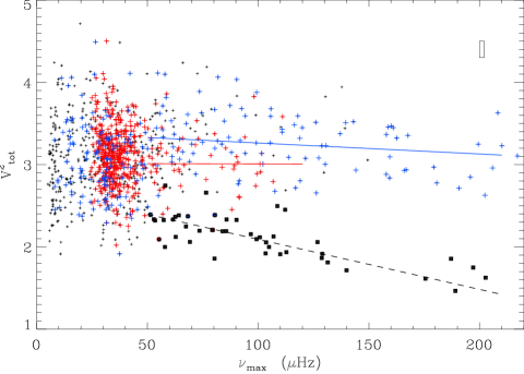
Figure 14: Visibility $V^{2}_{\mathrm{tot}}$ as a function of $\nu_{\mathrm{max}}$. Same color code as in Fig. 11. The fits of RGB, clump and low $V^{2}_{1}$ stars, in blue and red solid lines or black dashed line, respectively, are computed for $\nu_{\mathrm{max}}\geq 50\,\mu$Hz.

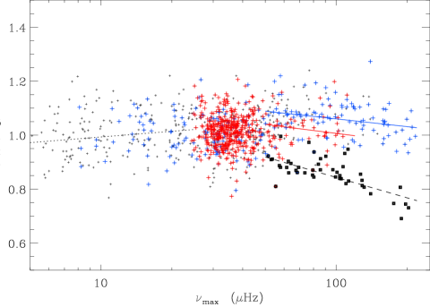
Figure 15: Ratio $\langle A\rangle/\langle A_{0}^{2}\rangle^{1/2}$ as a function of $\nu_{\mathrm{max}}$. Same color code as in Fig. 11. The fits of RGB, clump and low $V^{2}_{1}$ stars, in blue, red, and black, respectively, are valid at $\nu_{\mathrm{max}}\geq 50\,\mu$Hz. The dotted line indicates the fit at frequency lower than 30 $\mu$Hz.

7.4 Total visibility and radial amplitudes

We have estimated the total visibility $V^{2}_{\mathrm{tot}}=\sum_{\ell=0}^{3}V^{2}_{\ell}$ and note a large spread of the values, with RGB and clump stars having different mean values (Fig. 14). We also note that the stars with a low $V^{2}_{1}$ also show a low total visibility. Ballot et al. (2011) have calculated red giant limb-darkening functions, and derived a mean value $V^{2}_{\mathrm{tot}}\simeq 3.18$ for $T_{\mathrm{eff}}=4\,800$ K and solar metallicity. We find a mean value of about 3.06, in better agreement with the value 3.04 calculated by Bedding et al. (2010).

The mean value of $V^{2}_{\mathrm{tot}}$ can be used to improve the coefficient defining the globally averaged amplitude $\langle A\rangle$ given by Eq. 11. However, this globally averaged value is only indicative, due to the dispersion in $V^{2}_{\mathrm{tot}}$ (Fig. 14). This limits the use of $\langle A\rangle$ for deriving precise red giant radial amplitudes. Therefore, we discourage using the globally averaged value $\langle A\rangle$ for estimating the bolometric amplitude of a given red giant. Using $\langle A\rangle$ instead of $\langle A_{0}^{2}\rangle^{1/2}$ for establishing scaling relations is possible, but with an uncertainty on the exponent in $L$ of about 0.04. This value results from the differences in the slopes observed in the scaling relation of $\langle A\rangle/\langle A_{0}^{2}\rangle^{1/2}$ to $\nu_{\mathrm{max}}$ (Fig. 15), taking into account the fact that $L\propto\nu_{\mathrm{max}}$.

8 Conclusion

With Kepler photometric data recorded up to Q7, providing 590-day long time series, we have determined scaling relations of the global parameters that describe the oscillation power excess of red giants. About 1200 red giants were analyzed.

8.1 Global parameters and scaling relations

We have compared different methods, and shown that the background modelling influences the results. This influence does not prevent firm conclusions, but certainly needs further work to fully disentangle the fit of the granulation background from the oscillation power excess. There are indications that Harvey components with an exponent of 2 are sufficient for modelling the background of red giant spectra in the frequency range around $\nu_{\mathrm{max}}$.

We have found a significant influence of the red giant evolutionary status on the scaling relations describing the asteroseismic and fundamental stellar parameters. Following Mosser et al. (2011a), we show that red-clump stars have a mass distribution clearly linked to the seismic parameter $\nu_{\mathrm{max}}$, hence to the stellar radius. Therefore, the scaling relations expressed as a single power law of $\nu_{\mathrm{max}}$ present a large dispersion around the clump.

As a consequence of the different mass distributions, red giants on the RGB have larger oscillation amplitudes than the clump stars. Members of the secondary clump have different properties: compared to RGB stars, they have much higher masses, lower oscillation amplitudes, but with more modes excited.

We have compared the energy in the oscillations to its counterpart in the stellar background. The mean height in the oscillations is a fixed fraction of the energy density in the background at $\nu_{\mathrm{max}}$. This fraction depends only slightly on the evolutionary status. Since both granulation and oscillation are due to convection, such a result clearly indicates that the excitation mechanism of the oscillation has the same efficiency for a very large variety of red giants.

For both the background height and the bolometric amplitude, the agreement between the RGB and clump stars is better when considering in the scaling relations a mass dependence not exactly opposite to the luminosity dependence. The background height seems to scale as $L^{2}/M^{3}T_{\mathrm{eff}}^{5.5}$, as predicted by Kjeldsen & Bedding (2011).

8.2 Bolometric amplitudes and mode visibility

We have proposed a new method for deriving radial and non-radial amplitudes, and we have shown that the amplitudes obtained with a global integration are not appropriate for red giants, due to the presence of mixed modes that can significantly modify the total mode visibility.

Radial amplitudes have been translated into bolometric amplitudes for comparison with theoretical expectations. We have shown that current theoretical scaling relations are unable to provide an acceptable fit to the observed photometric amplitudes. There are strong observational indications in favor of an exponent in luminosity in the range [0.7, 0.8]. A negative exponent of the stellar mass larger, in absolute value, than the luminosity exponent helps to reduce the discrepancy between RGB and clump stars (Huber et al. 2011; Stello et al. 2011), but it seems that ingredients other than $L$ and $M$ are necessary to properly account for the observations.

We have also derived the mode visibility of $\ell$=1, 2 and 3 modes. The presence of mixed-modes reduces the observed values compared to expectations. As a result, we observe a new type of energy equipartition, where the squared amplitude of the pure pressure modes (as radial modes) seems to be shared by all mixed modes. We note a high dispersion that cannot be related to global parameters, and have identified a class of objects with very low $\ell=1$ amplitudes. It probably comprises red giants more massive than $1.3\,M_{\odot}$ where the coupling between pressure and gravity waves is so efficient that all $\ell=1$ mixed modes have a very high mode mass.

Appendix A Normalization of the power density spectra

Table 5: Characteristics of the different methods

pipeline	A2Za	CANb	CORc	OCTd	SYDe
spectrum	Lomb-Scargle periodogram $\to$ power density spectrum (PDS)
frequency axis	corrected for the duty cycle
frequency sampling	$\delta\nu=1/T$, with $T=N\;\delta t_{\mathrm{LC}}$ the total observation duration
	$\nu_{\mathrm{Nyquist}}=0.5/\delta t_{\mathrm{LC}}$, with $\delta t_{\mathrm{LC}}$ the Kepler long-cadence sampling
PDS normalization	$\sigma_{\nu}^{2}=2\,\sigma_{t}^{2}\ \delta t_{\mathrm{LC}}/N$
$\nu_{\mathrm{max}}$	centroid Gaussian
					or peak of the smoothed spectrum
smoothing	1$-\Delta\nu$ Gaussian filter	none	1$-\Delta\nu$ Gaussian filter
background	global	global	local	local	global
	Harvey	Harvey	$\propto\nu^{-\beta}$	second order polynomial	Harvey modified
value of exponent	free	4	free	2	2 and 4
number of components	2	3	1	1	2

References: $a)$ Mathur et al. (2010); $b)$ Kallinger et al. (2010); $c)$ Mosser & Appourchaux (2009); $d)$ Hekker et al. (2010); $e)$ Huber et al. (2009). For more information on the modelling of the background, see Mathur et al. (2011).

Different methods have been used and compared for the analysis of the power excess (Huber et al. 2009; Mosser & Appourchaux 2009; Hekker et al. 2010; Kallinger et al. 2010; Mathur et al. 2010). A comprehensive comparison of the properties and characteristics of the methods was given by Hekker et al. (2011a), but only dealt with the large separation $\Delta\nu$ and the frequency $\nu_{\mathrm{max}}$ of maximum oscillation signal. A comparison of complementary analysis methods applied to the Kepler short-cadence data by Verner et al. (2011) presented results on the maximum mode amplitude, but not for red giants. For the current work on red giants, parameters characterizing the oscillation power excess have been compared.

To ensure a correct comparison of results obtained with different methods, it was first necessary to normalize the outputs. The computation of power density spectra performed with Lomb-Scargle periodograms has taken into account the correction for the duty cycle of each target, in order to obtain spectra with the frequency resolution corresponding to the total observation time and frequency up to the Nyquist frequency ($\nu_{\mathrm{Nyquist}}=283.2\ \mu$Hz) related to the mean time sampling $\delta t_{\mathrm{LC}}$ of the Kepler long-cadence data. We chose to compute power density spectra (PDS) with the following normalization: a white noise signal recorded at the Kepler long-cadence sampling $\delta t_{\mathrm{LC}}$ with a noise level $\sigma_{\mathrm{t}}$ (in ppm) gives a PDS with a spectral density $\sigma_{\nu}$, such that $\sigma^{2}_{\nu}=2\sigma^{2}_{\mathrm{t}}\delta t_{\mathrm{LC}}/N$ where $N$ is the number of points in the time series. The characteristics of the methods used for this work are briefly described in Table 5.

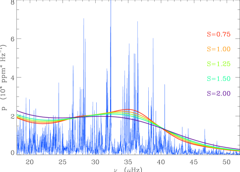
Figure 16: Influence of the width of the smoothing parameter for a typical red-clump giant (KIC 1161618). The different colors indicate the different values of the smoothing (in units of $\Delta\nu$).

Table 6: Influence of the smoothing on the seismic global parameters of KIC 1161618.

${\mathcal{S}}$	0.75	1	1.25	1.5	2
$\nu_{\mathrm{max}}({\mathcal{S}})\,/\,\nu_{\mathrm{max}}(1)$	1.00	1.00	0.98	0.97	0.96
$\delta\nu_{\mathrm{env}}({\mathcal{S}})\,/\,\delta\nu_{\mathrm{env}}(1)$	1.00	1.00	1.05	1.11	1.17
${H}_{\nu_{\mathrm{max}}}({\mathcal{S}})\,/\,{H}_{\nu_{\mathrm{max}}}(1)$	1.00	1.00	0.89	0.84	0.74
${B}_{\nu_{\mathrm{max}}}({\mathcal{S}})\,/\,{B}_{\nu_{\mathrm{max}}}(1)$	0.99	1.00	1.10	1.15	1.28
HBR$({\mathcal{S}})$ / HBR$(1)$	1.01	1.00	0.81	0.73	0.58
${\alpha_{B}}({\mathcal{S}})\,/\,{\alpha_{B}}(1)$	0.99	1.00	1.10	1.13	1.16

Appendix B Smoothing

Most of the methods use a smoothed spectrum to obtain the global parameters of the Gaussian envelope (Sect. 3). Since the width of the Gaussian envelope of red giant oscillation (Eq. 1) is narrow (Mosser et al. 2010), this step must be performed carefully. An example for a typical red-clump star is given in Fig. 16. The parameters ${H}_{\nu_{\mathrm{max}}}$ and ${B}_{\nu_{\mathrm{max}}}$ have been calculated for the local description of the background smoothed with different filter sizes and are summarized in Table 6. We have used a Gaussian window for performing the smoothing and have tested different values ${\mathcal{S}}$ of the FWHM. The mean value of the large separation acts as a natural characteristic frequency, so we expressed the FWHM in units of $\Delta\nu$ and have tested values varying from $0.75\,\Delta\nu$ to $2.0\,\Delta\nu$. When this value increases, the measured value of $\nu_{\mathrm{max}}$ decreases, with variations as large as 4 %, depending on the method. In parallel, ${H}_{\nu_{\mathrm{max}}}$ decreases and ${B}_{\nu_{\mathrm{max}}}$ increases when the filter width increases, which results in variations of the height-to-background ratio (HBR) larger than a factor of two. As expected, $\delta\nu_{\mathrm{env}}$ also increases with ${\mathcal{S}}$. This variation can be easily understood by recognizing that increasing the smoothing will spread the power of the oscillations relative to the background. We consider an acceptable compromise to be a Gaussian filter with a FWHM equal to the mean large separation $\Delta\nu$. Such a width is large enough for smoothing the influence of individual contributions of different degrees, and narrow enough to avoid the dilution of the global parameters, as shown by the example given in Table 6: when the parameter ${\mathcal{S}}$ gets larger than 1, all terms show significant variations.

This study shows the importance of the smoothing parameter. A systematic variation induced by the smoothing as large as 4 % in $\nu_{\mathrm{max}}$ is important because this parameter plays a key role in scaling relations for seismic parameters (Mosser et al. 2010; Huber et al. 2010). Since $\nu_{\mathrm{max}}$ is used for deriving the seismic mass and radius (Mosser et al. 2010; Kallinger et al. 2010; Hekker et al. 2011b), a bias should be avoided in order to avoid subsequent biases in the stellar parameters. A systematic relative error ${\sigma}_{\nu_{\mathrm{max}}}$ on $\nu_{\mathrm{max}}$ translates into a bias in the determination of the derived stellar parameters, of the order of ${\sigma}_{\nu_{\mathrm{max}}}$ and $3\,{\sigma}_{\nu_{\mathrm{max}}}$ for, respectively, the relative precision of the radius and mass.

A variation of a factor of two of the HBR depending on the smoothing means that studying the partition of energy between the oscillation and the background requires a careful description. According to the solar example, longer time-series are certainly required to reach the necessary precision to draw firm conclusions.

Appendix C Mode identification

The determination of the mode visibility (Sect. 4 and 7) requires the complete identification of the p-mode spectrum. This is automatically given by the red giant universal oscillation pattern (Mosser et al. 2011b), with the parametrization of the dimensionless factor $\varepsilon$ of the asymptotic development (Tassoul 1980). The function $\varepsilon(\Delta\nu)$ enables the identification of the radial modes

$$\nu_{n,\ell=0}=[n+\varepsilon(\Delta\nu)]\;\Delta\nu,$$ (16)

with $\Delta\nu$ the large separation averaged in the frequency range $[\nu_{\mathrm{max}}-\delta\nu_{\mathrm{env}},\nu_{\mathrm{max}}+\delta\nu_{\mathrm{env}}]$. For simplicity, we introduce the reduced frequency, dimensionless and corrected for the $\varepsilon$ term of the Tassoul equation:

$$n^{\prime}=\nu/\Delta\nu-\varepsilon(\Delta\nu).$$ (17)

According to Huber et al. (2010) and Mosser et al. (2011b), $\varepsilon$ is mainly a function of the large separation. For radial modes, the reduced frequency is very close to the radial order, except for possible very small secondary-order terms in $\varepsilon(\Delta\nu)$ that do not depend directly on $\Delta\nu$ and do not hamper the mode identification.

The determination of the evolutionary status of the giants (Sect. 4.2), namely the measurement of the g-mode spacing of $\ell=1$ mixed modes, is then achieved with the automated method described by Mosser et al. (2011a). This could be done for about 674 targets out of 1043 with high signal-to-noise ratio time series. This method measures the g-mode spacing of the mixed modes from the Fourier spectrum of the oscillation spectrum windowed with narrow filters centered on the expected locations of each pure $\ell=1$ pressure mode.