Phase diagram of iron-pnictides if doping acts as a disorder

Abstract

We obtain and analyze the phase diagram of doped iron-pnictides under the assumption that doping adds non-magnetic impurities to the system but does not change the densities of carriers. We show that the phase diagram is quite similar to the one obtained under the opposite rigid band assumption. In both cases, there is a phase where $s^{\pm}$ superconductivity and antiferromagnetism co-exist. We evaluate the jump of the specific heat, ${\mbox{\footnotesize$\Delta$}}C$, at the superconducting $T_{c}$ across the phase diagram and show that ${\mbox{\footnotesize$\Delta$}}C/T_{c}$ is non-monotonic, with the maximum at the onset of the co-existence phase. Our results are in quantitative agreement with experiments on some iron-pnictides.

I Introduction

How chemical doping of iron-pnictides affects their electronic structure is not fully understood yet and is subject of debates. In most studies it is assumed that doping does not affect the rigid band picture and only changes the densities of holes and electrons Hirschfeld et al. (2011). An alternative scenarioWadati et al. (2010) is that doping does not affect the carrier density but rather introduces non-magnetic impurities and hence increases disorder. Angle-resolved photoemission (ARPES) experiments on 122 materials Ba(Fe_1-xCo_x)₂As₂ and Ba_1-xK_xFe₂As₂ are usually interpreted in favor of the rigid band scenario. Within this scenario, if magnetism prevails at zero doping, the system moves from a spin-density-wave (SDW) phase to a superconducting (SC) state, and for some model parameters there is a mixed phase, where SDW and SC orders co-exist.Fernandes et al. (2010); Vorontsov et al. (2009); Cvetkovic and Tesanovic (2009) Recent ARPES experiments on Ru–doped BaFe₂As₂, however, found Brouet et al. (2010); Dhaka et al. (2011) that substitution of Fe with Ru practically does not change the Fermi surface (FS), yet the phase diagram is quite similar to that in other doped 122 materials: as Ru concentration increases, the system moves from an SDW phase to an SC phase. In between, there is a region where where both SDW and SC orders co-exist, although microscopic co-existence (as opposed to phase separation) has not been experimentally proven yet.Kaminski. (2011) Because FS geometry does not change, it seems natural to assume that the changes in the phase diagram caused by Ru-substitution are predominantly due to dilution and disorder associated with it. We also note that disorder may be introduced directly to pnictide materials by irradiation. Tarantini et al. (2010); Kim et al. (2010)

In the present paper, we address the issue of what is the phase diagram of a doped 122 Fe-pnictide if doping does not affect the carrier density but rather introduces non-magnetic impurities. We show that the phase diagram is actually the same as in the rigid band scenario. Namely, as doping increases, first an SDW phase becomes a mixed phase, then the system becomes a pure $s^{\pm}$ SC, and at even larger dopings $s^{\pm}$ SC is destroyed by disorder. This result may look somewhat counter-intuitive because non-magnetic impurities are pair-breaking for an $s^{\pm}$ SC. It turns out, however, that impurities damage SDW order stronger than they damage $s^{\pm}$ SC because both intra and inter-band impurity scattering is destructive for SDW, kul while only inter-band scattering is pair-breaking for an $s^{\pm}$ SC.Dolgov et al. (2009); Vorontsov et al. (2009); Bang (2009) Because of this disparity, the actual magnetic $T_{s}$ becomes smaller than the superconducting $T_{c}$ when the density of impurities exceeds a certain threshold, even for the undoped case $T_{s}>T_{c}$. There is no a’priori guarantee that a mixed state emerges near the point where $T_{s}=T_{c}$, i.e. a first order transition from an SDW to a SC is another option. Our calculation shows that the mixed state does appear, see Fig. 1a. For such a phase diagram to emerge, the magnetic SDW $T_{s,0}$ for undoped material should not be too strong compared to $T_{c,0}$, see below. If $T_{s,0}/T_{c,0}$ is too large, $T_{s}$ remains higher than $T_{c}$ down to $T_{c}\to 0$, even though $T_{s}$ decreases faster.

There is another reason to analyze the phase diagram assuming that doping introduces disorder. The measurements of the specific heat jump ${\mbox{\footnotesize$\Delta$}}C$ at $T_{c}$ across the phase diagram have demonstrated Bud’ko et al. (2009); Hardy et al. (2010a, b); Wang et al. (2008) that ${\mbox{\footnotesize$\Delta$}}C/T_{c}$ is non-monotonic and has a maximum at optimal doping that almost coincides with the onset of the co-existence phase. The slopes of ${\mbox{\footnotesize$\Delta$}}C/T_{c}$ are similar, although not exactly identical, upon deviations from optimal doping into both directions. This similarity raised speculations that the behavior of ${\mbox{\footnotesize$\Delta$}}C/T_{c}$ in underdoped and overdoped regimes may be related. Within the rigid band model, ${\mbox{\footnotesize$\Delta$}}C/T_{c}$ has a peak at the onset of a mixed phase and rapidly decreases at lower doping. Vavilov et al. (2011) However, the reduction of ${\mbox{\footnotesize$\Delta$}}C/T_{c}$ at higher doping cannot be straightforwardly explained within the rigid band model.

In the disorder model, the behavior of ${\mbox{\footnotesize$\Delta$}}C/T_{c}$ across the whole phase diagram is determined by a single parameter, the density of impurities $n_{\rm imp}$, and the forms of ${\mbox{\footnotesize$\Delta$}}C/T_{c}$ in the underdoped and overdoped regimes are related. We find that in the disordered model, ${\mbox{\footnotesize$\Delta$}}C/T_{c}$ indeed decreases on both sides of optimal doping, as shown in Figs. 1b and 2. The specific heat is discontinuous at the onset of the mixed phase within the mean field approximation, but becomes rounded once fluctuations are taken into account. The decrease of ${\mbox{\footnotesize$\Delta$}}C/T_{c}$ away from the maximum shows rather similar, although not identical, behavior in under- and over-doped regimes, with roughly quadratic dependence on the transition temperature $T_{c}$, see Fig. 2b. This behavior is in quantitative agreement with experiments.Bud’ko et al. (2009); Hardy et al. (2010a, b)

The fact that the phase diagram and the behavior of ${\mbox{\footnotesize$\Delta$}}C/T_{c}$ are similar in the rigid band and the disorder models is encouraging, since the two models are complementary to each other. In general, a chemical doping acts in both ways: (1) doping introduces some extra carriers and (2) increases impurity density. The relative magnitude of the two effects depends on materials. We argue in this regard that quite similar behavior observed in Ru, Co, and K - doped BaFe₂As₂ Bud’ko et al. (2009); Hardy et al. (2010a, b); Wang et al. (2008) is not a coincidence but rather a quite generic feature of iron-pnictides.

The paper is organized as follows. In the next section we discuss the model and introduce SDW and SC order parameters and describe the formalism used for calculations. In Sec. III we analyze the phase diagram as a function of impurity concentration, by solving linearized gap equation for one order parameter, SDW or SC, when the second parameter is either absent or present. Section IV presents calculations of the superconducting order parameter near the transition to a superconducting state. In Sec. V, we consider specific heat jump at the onset of superconductivity. We provide our conclusions in Sec. VI.

II The model

II.1 General formulation

Our goal is to demonstrate that the phase diagram remains the same if we associate doping with disorder rather than with the changes to the FS in the rigid band picture. We adopt the same minimal model that was used in earlier works within the rigid band approach.Vavilov et al. (2011) Namely, we consider a two band metal with cylindrical FSs for electron and hole-type excitations. The cylindrical FSs have circular cross-sections of equal radii centered at $(0,0)$ with a hole–like dispersion and $\bm{Q}=(0,\pi)$ with an electron–like dispersion. The free fermion part of the Hamiltonian in this case of perfect nesting is represented by

$${\cal H}_{0}=-\sum_{\bm{p},\alpha}\xi(\bm{p})\hat{c}_{\bm{p}\alpha}^{\dagger}\hat{c}_{\bm{p}\alpha}+\sum_{{\bm{p}},\alpha}\xi(\tilde{\bm{p}})\hat{f}_{\tilde{\bm{p}}\alpha}^{\dagger}\hat{f}_{\tilde{\bm{p}}\alpha},$$

where operators $\hat{c}$ annihilate hole–like fermions near $(0,0)$ and operators $\hat{f}$ annihilate electron–like fermions near $\bm{Q}$. The fermionic dispersion is given by $\xi(\bm{p})=\bm{p}^{2}/2m-\mu$, and the momentum $\tilde{\bm{p}}$ of electron excitations is measured as a deviation from $\bm{Q}$, $\tilde{\bm{p}}=\bm{p}-\bm{Q}$.

We consider an effective low-energy theory with the high-energy cutoff $\Lambda$ and angle-independent interactions in the SDW channel and in the $s^{\pm}$ SC channel with the couplings $\lambda_{\rm sdw}$ and $\lambda_{\rm sc}$.Vorontsov et al. (2009); Chubukov et al. (2008); Maiti and Chubukov (2010); Wang et al. (2009); Thomale et al. (2009); Platt et al. (2009) We treat these interactions within a mean field approximation, by introducing SC and SDW order parameters, $\Delta$ and ${\bf M}$, respectively, and decomposing the four-fermion interactions into effective quadratic terms with $\Delta$ and ${\bf M}$ in the prefactors. The full mean-field Hamiltonian is quadratic in fermionic operators and can be written as

$${\cal{H}}=\frac{1}{2}\sum_{\bm{p},\alpha,\beta}\overline{\Psi}_{\bm{p},\alpha}\hat{H}_{\bm{p},\alpha,\beta}\Psi_{\bm{p},\beta},$$ (1)

where $\overline{\Psi}_{\bm{p},\alpha}=(\hat{c}^{\dagger}_{\bm{p},\alpha},\ \hat{c}_{-\bm{p},\alpha},\ \hat{f}^{\dagger}_{\bm{p},\alpha},\ \hat{f}_{-\bm{p},\alpha})$ and $\Psi_{\bm{p},\alpha}$ is a conjugated column. The Hamiltonian matrix $\hat{H}_{\bm{p},\alpha,\beta}$ can be written in the formVorontsov et al. (2009)

$$\begin{split}\hat{H}&=\hat{H}_{0}+\hat{H}_{\rm mf};\quad\hat{H}_{0}=-\xi\hat{\tau}_{3}\hat{\rho}_{3}\hat{\sigma}_{0}\\ \hat{H}_{\rm mf}&=-\Delta\hat{\tau_{2}}\hat{\rho}_{3}\hat{\sigma}_{2}+\hat{\tau}_{3}\hat{\rho}_{1}(\bm{M}\hat{\bm{\sigma}}).\end{split}$$ (2)

Here, the Pauli matrices $\hat{\tau}_{i}$, $\hat{\rho}_{i}$ and $\hat{\sigma}_{i}$ are defined in the Gorkov-Nambu, band, and spin spaces, respectively, where $i=0,1,2,3$ and matrices with $i=0$ are unit matrices. A fermion Green’s function $\hat{G}(\omega_{n},\bm{p})$ is defined as a solution to

$$\left(i\omega_{n}-\hat{H}_{\bm{p}}-\hat{\Sigma}\right)\hat{G}(\omega_{n},\bm{p})=\hat{1},$$ (3a)

and the conjugated equation is

$$\hat{G}(\omega_{n},\bm{p})\left(i\omega_{n}-\hat{H}_{\bm{p}}-\hat{\Sigma}\right)=\hat{1}.$$ (3b)

Here $\hat{\Sigma}$ is the self energy for scattering off disorder and $\omega_{n}=2\pi T_{m}(n+1/2)$ with integer $n$ are Matsubara frequencies.

We describe disorder scattering within the Born approximation and assume that the Born scattering amplitude $U(\bm{q})$ is characterized by a constant $U_{0}$ for scattering within the same band and $U_{\pi}$ for scattering between the two bands.Dolgov et al. (2009); Vorontsov et al. (2009); Bang (2009) In this approximation, the self-energy is

$$\begin{split}\hat{\Sigma}(\omega_{n})=&\frac{4\Gamma_{0}}{\pi N_{F}}\int\frac{d\bm{p}}{(2\pi\hbar)^{2}}\hat{\tau}_{3}\hat{\rho}_{0}\hat{\sigma}_{0}\hat{G}(\omega_{n},\xi)\hat{\tau}_{3}\hat{\rho}_{0}\hat{\sigma}_{0}\\ +&\frac{4\Gamma_{\pi}}{\pi N_{F}}\int\frac{d\bm{p}}{(2\pi\hbar)^{2}}\hat{\tau}_{3}\hat{\rho}_{1}\hat{\sigma}_{0}\hat{G}(\omega_{n},\xi)\hat{\tau}_{3}\hat{\rho}_{1}\hat{\sigma}_{0}.\end{split}$$ (4)

where we introduced disorder scattering rates

$$\Gamma_{0}=\frac{\pi N_{F}n_{\rm imp}}{4}|U_{0}|^{2},\quad\Gamma_{\pi}=\frac{\pi N_{F}n_{\rm imp}}{4}|U_{\pi}|^{2}.$$ (5)

$\Gamma_{0}$ characterizes the rate of electron collisions with impurities in which the electron remains in its original band, while $\Gamma_{\pi}$ is the rate of collisions resulting in electron transfer between the two bands. $N_{F}$ in Eq. (5) is the total quasiparticle density of states (DoS) at the Fermi energy ( the DoS per spin per band is $N_{F}/4$). We assume that only the impurity density $n_{\rm imp}$ changes with doping, i.e., the ratio $\Gamma_{\pi}/\Gamma_{0}$ is doping independent.

The two mean-field parameters $\Delta$ and ${\bf M}$ are obtained self-consistently via the matrix Green’s function as

$$\frac{\Delta}{\lambda_{\rm sc}}=\frac{T}{2}\sum_{\omega_{n}}\int\frac{d\bm{p}}{(2\pi\hbar)^{2}}{\rm Tr}\left\{\hat{G}(\omega_{n},\bm{p})\hat{\tau}^{+}\left(\hat{\rho}_{0}+\hat{\rho}_{3}\right)\hat{\sigma}^{+}\right\},$$ (6)

and

$$\frac{\bm{M}}{\lambda_{\rm sdw}}=\frac{T}{4}\sum_{\omega_{n}}\int\int\frac{d\bm{p}}{(2\pi\hbar)^{2}}{\rm Tr}\left\{\hat{G}(\omega_{n},\bm{p})\left(\hat{\tau}_{0}+\hat{\tau}_{3}\right)\hat{\rho}^{+}\hat{\bm{\sigma}}\right\},$$ (7)

where $\hat{A}^{+}=(\hat{A}_{1}+i\hat{A}_{2})/2$ for $\hat{A}\to\hat{\rho},\hat{\tau},\hat{\sigma}$.

For the pure SDW and the pure $s^{+-}$ SC state in the absence of disorder, the solution of the linearized gap equations yield transition temperatures $T_{s,0}=1.13\Lambda\exp(-2/(N_{F}\lambda_{\rm sdw}))$ and $T_{c,0}=1.13\Lambda\exp(-2/(N_{F}\lambda_{\rm sc}))$. We consider $T_{s,0}>T_{c,0}$, so that without disorder the SDW phase develops at a higher temperature.

II.2 Eilenberger equation

To treat superconductivity and magnetism in the presence of disorder, it is convenient to introduce the Eilenberger’s Green function

$$\hat{\cal{G}}(\omega_{n})=\frac{4i}{\pi N_{F}}\int\frac{d\bm{p}}{(2\pi\hbar)^{2}}\hat{\tau}_{3}\hat{\rho}_{3}\hat{\sigma}_{0}\hat{G}(\omega_{n},\bm{p})$$ (8)

which appears both in the self-consistency equations, Eqs. (6) and (7), and in the expression for the impurity self-energy, Eq. (4). In particular, the impurity self energy is

$$\begin{split}\hat{\Sigma}&=-i\Gamma_{0}\hat{\tau}_{0}\hat{\rho}_{3}\hat{\sigma}_{0}\hat{\cal G}\hat{\tau}_{3}\hat{\rho}_{0}\hat{\sigma}_{0}-i\Gamma_{\pi}\hat{\tau}_{0}(-i\hat{\rho}_{2})\hat{\sigma}_{0}\hat{\cal G}\hat{\tau}_{3}\hat{\rho}_{1}\hat{\sigma}_{0}.\end{split}$$ (9)

To derive the equation for $\hat{\cal{G}}$, we multiply Eq. (3a) by $\hat{\tau}_{3}\hat{\rho}_{3}$ from left and subtract Eq. (3b), multiplied by $\hat{\tau}_{3}\hat{\rho}_{3}$ from right. We then multiply the resulting equation by $\hat{\tau}_{3}\hat{\rho}_{3}$ from left again. As a result, the $\hat{H}_{0}(\bm{p})$ term falls out. We integrate the resulting equation over $\bm{p}$ and obtain the equation for $\hat{\cal{G}}(\omega_{n})$ in the form of a commutator:

$$\left[i\omega_{n}\hat{\tau}_{3}\hat{\rho}_{3}\hat{\sigma}_{0}-(\hat{H}_{\rm mf}+\hat{\Sigma})\hat{\tau}_{3}\hat{\rho}_{3}\hat{\sigma}_{0};\hat{\cal{G}}(\omega_{n})\right]=0.$$ (10)

This equation is the Eilenberger equation,Eilenberger (1968); Moor et al. (2011) obtained for a two-band metal with homogeneous in space SDW and SC order parameters. The Eilenberger equation is consistent with the normalization relations for $\hat{\cal{G}}$: $\rm{Tr}\hat{\cal{G}}(\omega_{n})=0$ and $\hat{\cal{G}}(\omega_{n})\hat{\cal{G}}(\omega_{n})=\hat{1}$.

Without loss of generality, we direct $\bm{M}$ along $z$–axis and parametrize the matrix $\hat{\cal{G}}(\omega_{n})$ by the three functions $g_{\omega_{n}}$, $f_{\omega_{n}}$ and $S_{\omega_{n}}$ as

$$\hat{\cal{G}}(\omega_{n})=g_{\omega_{n}}\hat{\tau}_{3}\hat{\rho}_{3}\hat{\sigma}_{0}+f_{\omega_{n}}\hat{\tau}_{1}\hat{\rho}_{0}(-i\hat{\sigma}_{2})+S_{\omega_{n}}\hat{\tau}_{0}(-i\hat{\rho}_{2})\hat{\sigma}_{3}.$$ (11)

The function $g_{\omega_{n}}$ is the normal component of the Eilenberger Green’s function, while the functions $S_{\omega_{n}}$ and $f_{\omega_{n}}$ are the two anomalous components, associated with the SDW and SC orders, respectively.

For the above parametrization of $\hat{\cal G}(\omega_{n})$, Eq. (11), the normalization condition $\hat{\cal{G}}\hat{\cal{G}}=1$ reduces to

$$g_{\omega_{n}}^{2}-S_{\omega_{n}}^{2}-f_{\omega_{n}}^{2}=1,$$ (12)

and the commutation relation Eq. (10) gives

$$i\Delta g_{\omega_{n}}=f_{\omega_{n}}(\omega_{n}+2\Gamma_{\pi}g_{\omega_{n}}),$$ (13a)

$$iMg_{\omega_{n}}=S_{\omega_{n}}(\omega_{n}+2\Gamma_{t}g_{\omega_{n}}).$$ (13b)

where $\Gamma_{t}=\Gamma_{0}+\Gamma_{\pi}$.

The self-consistency equations for SDW and SC order parameters, Eqs. (6) and (7), can be rewritten in terms of anomalous SDW and SC components of the Eilenberger’s Green function as

$$\frac{2M}{N_{F}\lambda_{\rm sdw}} = -i~{}2\pi T\sum_{\omega_{n}>0}^{\Lambda}S_{\omega_{n}},\quad$$ (14a)

$$\frac{2\Delta}{N_{F}\lambda_{\rm sc}} = -i~{}2\pi T\sum_{\omega_{n}>0}^{\Lambda}f_{\omega_{n}}.$$ (14b)

III Phase diagram

We first consider pure SDW and SC states. For a pure SDW state we set $\Delta=0$ and $f_{\omega_{n}}=0$ in Eqs. (12) and (13a), linearize Eq. (13b) in $M$ and find from Eq. (14a) that the SDW transition temperature $T_{s}$ evolves with doping as

$$\frac{2}{N_{F}\lambda_{\rm sdw}}=2\pi T_{s}\sum_{n\geq 0}^{\Lambda/2\pi T_{s}}\frac{1}{\pi T_{s}(2n+1)+2\Gamma_{t}}.$$ (15)

This equation can be rewritten in terms of the transition temperature $T_{s,0}$ to SDW phase at $\Gamma_{t}=0$ as

$$\ln\frac{T_{s,0}}{T_{s}}=\psi\left(\frac{1}{2}+\frac{\Gamma_{t}}{\pi T_{s}}\right)-\psi\left(\frac{1}{2}\right),$$ (16)

where $\psi(x)$ is the digamma function.kul

For a pure SC state we set $M=0$ and $S_{\omega_{n}}=0$ in Eqs. (12) and (13b) and linearize Eq. (13a) in $\Delta$. We obtain from Eq. (14b)

$$\frac{2}{N_{F}\lambda_{\rm sc}}=2\pi T_{c}\sum_{n\geq 0}^{\Lambda/2\pi T_{c}}\frac{1}{\pi T_{c}(2n+1)+2\Gamma_{\pi}}.$$ (17)

Re-expressing the result in terms of the superconducting transition temperature $T_{c,0}$ in a clean system and without SDW, we re-write Eq. (17) as

$$\ln\frac{T_{c,0}}{T_{c}}=\psi\left(\frac{1}{2}+\frac{\Gamma_{\pi}}{\pi T_{c}}\right)-\psi\left(\frac{1}{2}\right),$$ (18)

which is similar to the equation for $T_{c}$ in conventional $s-$wave superconductors with magnetic impuritiesAbrikosov and Gorkov (1961) and in unconventional $d-$wave superconductors with potential impurities.Balatsky et al. (2006); Galitski (2008); Vorontsov et al. (2010) Note that only inter-band scattering $\Gamma_{\pi}$, is pair-breaking for $s^{\pm}$ SC.

Even if $T_{s,0}>T_{c,0}$, $T_{s}$ decreases faster than $T_{c}$ with increasing $n_{\rm imp}$, and at certain doping the two transition temperatures may cross. We denote this temperature as $T_{P}$. The condition that $T_{P}$ exists, i.e. that $T_{c}$ and $T_{s}$ cross before $T_{c}\to 0$, sets the limits on the ratios $T_{s,0}/T_{c,0}$ and $\Gamma_{\pi}/\Gamma_{0}$. We find that $T_{s}$ and $T_{c}$ cross if $T_{c,0}/T_{s,0}>1/(1+\Gamma_{0}/\Gamma_{\pi})$. For on-cite disorder potential $\Gamma_{\pi}=\Gamma_{0}$, and $T_{P}>0$ exists, i.e. SC phase exists, if $T_{c,0}/T_{s,0}>1/2$. For longer-range impurity potentials, $\Gamma_{0}>\Gamma_{\pi}$, and the SC phase develops even for smaller $T_{c,0}/T_{s,0}$, see Figs. 1a and 3a.

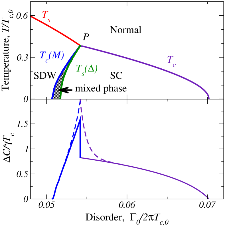
Figure 1: (Color online) Upper panel: The phase diagram as a function of disorder, measured in units $\Gamma_{0}/2\pi T_{c,0}\propto n_{\rm imp}$, for on-site disorder ($\Gamma_{\pi}=\Gamma_{0}$), and $T_{s,0}/T_{c,0}=1.7$. The four transition lines terminate at a tetra-critical point $P$, where normal, pure SDW, pure SC, and mixed phase meet. The shaded region represents the mixed phase. Lower panel: Specific heat jump ${\mbox{\footnotesize$\Delta$}}C/T_{c}$ as a function of doping. Solid curves represent the mean field result and the dashed curve illustrates the effect of thermodynamic fluctuations beyond the mean field theory.

To obtain the superconducting transition temperature $T_{c}(M)$ in the presence of pre-existing magnetism one has to solve the linearized equation for $\Delta$ at a finite $M$. Now $g_{\omega_{n}}$ depends on $M$ (i.e., $g_{\omega_{n}}=g_{\omega_{n}}(M)$), and we have from Eq. (14b)

$$\alpha(T_{c}(M))=\frac{2}{N_{F}\lambda_{sc}},$$ (19)

where

$$\alpha(T)=2\pi T\sum_{\omega_{n}>0}^{\Lambda}\frac{g_{\omega_{n}}(M)}{\omega_{n}+2\Gamma_{\pi}g_{\omega_{n}}(M)}.$$ (20)

The temperature dependence in the r.h.s. of Eq. (20) is via $\omega_{n}=\pi T(2n+1)$ and also via $g_{\omega_{n}}(M)$ because $M$ depends on temperature. The summation in $\alpha(T)$ has a logarithmic dependence on the high-energy cut-off $\Lambda$. This dependence can be eliminated in favor of the transition temperature $T_{c}$ at $M=0$. Subtracting Eq. (17) from Eq. (19), we obtain after a simple algebra an equation on $T_{c}(M)$ in the form

$$\begin{split}{\cal L}(T_{c}(M),T_{c},\Gamma_{\pi})=\sum_{\omega_{n}>0}^{\Lambda}\frac{2\pi T_{c}(M)\omega_{n}[g_{\omega_{n}}(M)-1]}{(\omega_{n}+2\Gamma_{\pi})(\omega_{n}+2\Gamma_{\pi}g_{\omega_{n}}(M))},\end{split}$$ (21)

where

$$\begin{split}{\cal L}(T_{1},T_{2},\Gamma)=\ln\frac{T_{1}}{T_{2}}+\psi\left(\frac{1}{2}+\frac{\Gamma}{\pi T_{1}}\right)-\psi\left(\frac{1}{2}+\frac{\Gamma}{\pi T_{2}}\right).\end{split}$$ (22)

We calculate $g_{\omega_{n}}(M)$ as a function of temperature at a given impurity concentration. For this purpose, we express $S_{\omega_{n}}(M)$ in terms of $g_{\omega_{n}}(M)$ using Eq. (13b),

$$S_{\omega_{n}}(M)=\frac{iMg_{\omega_{n}}(M)}{\omega_{n}+2\Gamma_{t}g_{\omega_{n}}(M)},$$ (23)

substitute the result into Eq. (12) with $f_{\omega_{n}}=0$, and obtain the fourth–order algebraic equation for $g_{\omega_{n}}(M)$ as a function of $M$:

$$g_{\omega_{n}}^{2}(M)+\frac{M^{2}g_{\omega_{n}}^{2}(M)}{(\omega_{n}+2\Gamma_{t}g_{\omega_{n}}(M))^{2}}=1.$$ (24)

We solve this equation, obtain $g_{\omega_{n}}(M)$, substitute the result back into Eqs. (23) and (14a), utilize the definition of $T_{s}$, and obtain the non-linear equation for $M=M(T)$ in the form

$${\cal L}(T,T_{s},\Gamma_{t})=2\pi T\sum_{\omega_{n}>0}\frac{\omega_{n}\left[g_{\omega_{n}}(M)-1\right]}{(\omega_{n}+2\Gamma_{t})(\omega_{n}+2\Gamma_{t}g_{\omega_{n}}(M))},$$ (25)

where $g_{\omega_{n}}(M)$ is a solution of Eq. (24), one has to choose the branch with $g_{\omega_{n}}(M=0)=1$. Solving (25) we obtain $M(T)$, and hence $g_{\omega_{n}}(T)$. Substituting the result into (19) and (20) we obtain the superconducting transition temperature $T_{c}(M)$ in the mixed phase as a function of doping.

We numerically evaluate $T_{c}(M)$ at different dopings in the mixed phase and plot the result in Figs. 1a and 3a. As the doping decreases from its optimal value, $M$ increases at a given temperature $T$, and $T_{c}(M)$ rapidly drops. This is expected since SDW and SC order parameters compete with each other. At $M\to 0$, $g_{\omega_{n}}(M)\to 1$ and Eq. (21) yields $T_{c}(M)\to T_{c}$, as expected.

A similar calculation of the SDW transition temperature from the preexisting SC phase, $T_{s}(\Delta)$, shows that $T_{s}(\Delta)$ decreases as $\Delta$ increases, due to the same kind of competition. Furthermore, the $T_{s}(\Delta)$ curve actually bends toward smaller dopings, see Figs. 1a and 3a, so that with decreasing temperature the system moves from a pure SDW magnet to a pure superconductor through a mixed phase. The bending of the $T_{s}(\Delta)$ curve is in agreement with the general analysis in Ref. Moon and Sachdev, 2010. The four curves $T_{c}$, $T_{c}(M)$, $T_{s}$, and $T_{s}(\Delta)$ meet at the tetracritical point $P$, as shown in Figs. 1a and 3a. The corresponding temperature $T_{P}$ is the highest superconducting transition temperature. We also see from numerics that, despite bending, the curve $T_{s}(\Delta)$ is always located to the right of the curve $T_{c}(M)$, i.e. if one increases disorder at a given $T$ or decreases $T$ at a given disorder, the system with the SDW order first becomes unstable toward an intermediate mixed phase where SDW and SC orders co-exist, and only then SDW order disappears.

The intermediate mixed phase was earlier found in the rigid band model. Fernandes et al. (2010); Vorontsov et al. (2009) However, in that model it only appears at a finite ellipticity of electron pockets, while for circular hole and electron FSs doping gives rise to a first order transition between pure SDW and pure SC phases. In the disorder model, the mixed phase appears already for circular hole and electron pockets and by continuity should also exists when electron pockets have weak ellipticity. We, however, did not analyze the whole range of ellipticities and therefore cannot exclude a possibility of a first order transition for strongly elliptical electron FSs.

IV Superconducting order parameter near $T_{c}$

We verified that the mixed phase does indeed exist in the disorder model with circular FSs by expanding in Eq. (13a) to order $\Delta^{3}$ and solving the equation for $\Delta$ in the presence of $\bm{M}$ at a temperature slightly below $T_{c}(M)$. The expansion yields, quite generally:

$$\alpha(T)-\beta\Delta^{2}=\frac{2}{\lambda_{\rm sc}N_{F}}$$ (26)

where $\alpha(T)$ is introduced in Eq. (20) and $\beta=\beta(T_{c}(M))$ is given by Eq. (37) below. Near $T_{c}(M)$, we have $\alpha(T)=\alpha(T_{c}(M))+\alpha^{\prime}(T_{c}(M))\left(T-T_{c}(M)\right)$ and $\alpha(T_{c}(M))$, see Eq. (19). On general grounds, $\alpha^{\prime}(T_{c}(M))$ must be negative for a SC phase to develop as $T$ decreases, and we indeed show below that $\alpha^{\prime}(T_{c}(M))<0$. The type of the transition is, however, determined by the sign of $\beta$. The mixed phase exists if $\beta>0$ because then $\Delta$ gradually grows as $T$ decreases. If $\beta<0$, $\Delta$ changes discontinuously around $T_{c}(M)$ and the SDW and SC phases are separated by the first-order transition. Fernandes et al. (2010); Vorontsov et al. (2009)

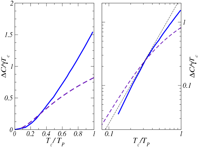
Figure 2: (Color online) The specific heat jump ${\mbox{\footnotesize$\Delta$}}C/T_{c}$ for $\Gamma_{\pi}=\Gamma_{0}$, and $T_{s,0}=1.7T_{c,0}$, as a function of $T_{c}/T_{P}$, where $T_{P}$ is the temperature of the tetra-critical point. Left panel: linear scale, right panel: log–log scale. The solid line represents the specific heat jump ${\mbox{\footnotesize$\Delta$}}C/T_{c}$ at $T_{c}(M)$ in the mixed phase in the underdoped regime, and the dashed line represents ${\mbox{\footnotesize$\Delta$}}C/T_{c}$ in the overdoped regime, where SDW order is absent. A thin dash line represents a quadratic dependence ${\mbox{\footnotesize$\Delta$}}C/T_{c}\propto T_{c}^{2}$.

The coefficient $\alpha(T)$ can be rewritten in the form of Eqs. (21) and (22):

$$\alpha(T)=\frac{2}{\lambda_{sc}N_{F}}-Y(T),\quad\alpha^{{}^{\prime}}(T)=-\frac{\partial Y(T)}{\partial T}$$ (27)

where

$$\begin{split}Y(T)&={\cal L}\left(T,T_{c},\Gamma_{\pi}\right)\\ &+\sum_{\omega_{n}>0}\frac{2\pi T\omega_{n}(1-g_{\omega_{n}}(M))}{[\omega_{n}+2\Gamma_{\pi}][\omega_{n}+2\Gamma_{\pi}g_{\omega_{n}}(M)]}.\end{split}$$ (28)

For $M=0$ and in the clean limit $\alpha^{\prime}(T_{c})=-1/T_{c}$. We verified numerically that $\alpha^{\prime}(T_{c}(M))$ remains negative at $M\neq 0$ and in the presence of disorder, as expected.

Calculations of $\beta$ require more care as one has to combine terms coming from the apearance of non-zero $f_{\omega_{n}}$ in Eq. (12) and from the expansion of the SDW order parameter $M(\Delta)$ to order $\Delta^{2}$ as $M(\Delta)=M+\delta M^{(2)}$, where $\delta M^{(2)}\propto\Delta^{2}$. Similarly, we introduce $g_{\omega_{n}}=g_{\omega_{n}}(M)+\delta g_{\omega_{n}}^{(2)}$ and $S_{\omega_{n}}=S_{\omega_{n}}(M)+\delta S_{\omega_{n}}^{(2)}$. Substituting $g_{\omega_{n}}$ and $S_{\omega_{n}}$ into Eqs. (12) and (13b), we obtain equations for $\delta g_{\omega_{n}}^{(2)}$ and $\delta S_{\omega_{n}}^{(2)}$:

$$\begin{split}g_{\omega_{n}}(M)\delta g_{\omega_{n}}^{(2)}-S_{\omega_{n}}(M)\delta S_{\omega_{n}}^{(2)}&=\frac{1}{2}[f_{\omega_{n}}^{(1)}]^{2},\\ \frac{-iM\omega_{n}\delta g_{\omega_{n}}^{(2)}}{(\omega_{n}+2\Gamma_{t}g_{\omega_{n}}(M))^{2}}+\delta S_{\omega_{n}}^{(2)}&=\frac{i\delta M^{(2)}g_{\omega_{n}}(M)}{\omega_{n}+2\Gamma_{t}g_{\omega_{n}}(M)},\end{split}$$ (29)

where

$$f_{\omega_{n}}^{(1)}=\frac{i\Delta g_{\omega_{n}}(M)}{\omega_{n}+2\Gamma_{\pi}g_{\omega_{n}}(M)}$$ (30)

and $g_{\omega_{n}}(M)$ is defined by Eq. (23). Solving Eq. (29) we obtain

$$\begin{split}\delta g_{\omega_{n}}^{(2)}&=-\frac{1}{2}\frac{g_{\omega_{n}}(M)(\omega_{n}+2\Gamma_{t}g_{\omega_{n}}(M))^{2}}{(\omega_{n}+2\Gamma_{t}g_{\omega_{n}}(M))^{3}+M^{2}\omega_{n}}\\ &\times\left(\Delta^{2}\frac{\omega_{n}+2\Gamma_{t}g_{\omega_{n}}(M)}{(\omega_{n}+2\Gamma_{\pi}g_{\omega_{n}}(M)^{2}}+\frac{2M\delta M^{(2)}}{\omega_{n}+2\Gamma_{t}g_{\omega_{n}}(M)}\right)\end{split}$$ (31)

and

$$\begin{split}\delta S_{\omega_{n}}^{(2)}&=-\frac{i}{2}\frac{g_{\omega_{n}}(M)(\omega_{n}+2\Gamma_{t}g_{\omega_{n}}(M))^{2}}{(\omega_{n}+2\Gamma_{t}g_{\omega_{n}}(M))^{3}+M^{2}\omega_{n}}\\ &\times\left(\frac{\Delta^{2}M\omega_{n}}{(\omega_{n}+2\Gamma_{\pi}g_{\omega_{n}}(M))^{2}(\omega_{n}+2\Gamma_{t}g_{\omega_{n}}(M))}-2\delta M^{(2)}\right).\end{split}$$ (32)

We first evaluate $\delta M^{(2)}$ by substituting $S_{\omega_{n}}=S_{\omega_{n}}^{(0)}+S_{\omega_{n}}^{(2)}$ into Eq. (14a) and eliminating the SDW coupling constant in favor of the SDW transition temperature $T_{s}$, see Eq. (15). We obtain

$$\delta M^{(2)}{\cal L}(T,T_{s},\Gamma_{t})=-2\pi T\sum_{\omega_{n}>0}\left(i\delta S_{\omega_{n}}^{(2)}+\frac{\delta M^{(2)}}{\omega_{n}+2\Gamma_{t}}\right).$$ (33)

Substituting ${\cal L}(T,T_{s},\Gamma_{t})\approx{\cal L}(T_{c}(M),T_{s},\Gamma_{t})$ from Eq. (25) and $\delta S_{\omega_{n}}^{(2)}$ from Eq. (32) we obtain

$$\delta M^{(2)}=-\frac{\Delta^{2}}{2M}\frac{C}{B},$$ (34)

where the coefficients $B$ and $C$, together with the term $A$ which we utilize below, are given by

$$A =\pi T\sum_{\omega_{n}>0}\frac{g_{\omega_{n}}(M)\omega_{n}(\omega_{n}+2\Gamma_{t}g_{\omega_{n}}(M))^{3}}{[\omega_{n}+2\Gamma_{\pi}g_{\omega_{n}}(M)]^{4}D},$$ (35a)

$$B =\pi T\sum_{\omega_{n}>0}\frac{g_{\omega_{n}}(M)\omega_{n}}{[\omega_{n}+2\Gamma_{t}g_{\omega_{n}}(M)]D},$$ (35b)

$$C =\pi T\sum_{\omega_{n}>0}\frac{g_{\omega_{n}}(M)\omega_{n}(\omega_{n}+2\Gamma_{t}g_{\omega_{n}}(M))}{[\omega_{n}+2\Gamma_{\pi}g_{\omega_{n}}(M)]^{2}D},$$ (35c)

$$D =[\omega_{n}+2\Gamma_{t}g_{\omega_{n}}(M)]^{3}+\omega_{n}M^{2}.$$ (35d)

Substituting $\delta M^{(2)}$ into (31) we obtain $\delta g^{(2)}\propto\Delta^{2}$.

We next write $f_{\omega_{n}}$, defined by Eq. (13a) to the third order in $\Delta$

$$f_{\omega_{m}}=\frac{i\Delta g_{\omega_{n}}(M)}{\omega_{n}+2\Gamma_{\pi}g_{\omega_{n}}(M)}+\frac{i\Delta\omega_{n}g_{\omega_{n}}^{(2)}}{(\omega_{n}+2\Gamma_{\pi}g_{\omega_{n}}(M))^{2}},$$ (36)

substitute this expression into Eq. (14b), and obtain Eq. (26) with

$$\beta=\left(A-\frac{C^{2}}{B}\right)$$ (37)

where $A,B$, and $C$ are given by Eq. (35).

Evaluating these coefficients, we find $AB>C^{2}$, i.e., $\beta$ is positive. This confirms our numerical result that the phase diagram of the disorder model contains the mixed phase where SDW and SC orders co-exist.

Equation (26) can also be applied to the transition from a paramagnetic metal into a pure SC state. In this case, $M=0$, and hence $g_{\omega_{n}}=g_{\omega_{n}}(M)=1$ and $C^{2}/B$ term in Eq. (37) is absent, i.e. $\beta=A$. Substituting $g_{\omega_{n}}(M)=1$ into Eqs. (35a) and (35d) we obtain

$$\alpha^{\prime}(T_{c}) =-\frac{1}{T_{c}}\left(1-\sum_{m=0}^{\infty}\frac{\Gamma_{\pi}/\pi T_{c}}{(m+1/2+\Gamma_{\pi}/\pi T_{c})^{2}}\right),$$ (38a)

$$\beta =\frac{1}{8\pi^{2}T^{2}_{c}}\sum_{m=0}^{\infty}\frac{m+1/2}{(m+1/2+\Gamma_{\pi}/\pi T_{c})^{4}},$$ (38b)

where $T_{c}$ is given by Eq. (18). Note that, again, $\alpha^{\prime}(T_{c})<0$ and $\beta>0$.

V Specific heat jump at the onset of superconductivity

The specific heat jump at $T_{c}$ and $T_{c}(M)$ can be obtained by evaluating the change in the thermodynamic potential $\delta\Omega$ imposed by superconductivity Abr

$${\mbox{\footnotesize$\Delta$}}\Omega=\int_{0}^{\Delta}\frac{d\lambda^{-1}_{\rm sc}}{d\Delta_{1}}\Delta_{1}^{2}d\Delta_{1}=-\frac{N_{F}\beta\Delta^{4}}{4},$$ (39)

where $d\lambda_{\rm sc}^{-1}/d\Delta$ and $\Delta^{2}$ are defined by Eq. (26). For $\Delta^{2}$ we have

$$\Delta^{2}=\frac{1}{\beta}\left(\alpha(T)-\frac{2}{\lambda_{\rm sc}N_{F}}\right)=\frac{|\alpha^{\prime}|}{\beta}(T_{c}(M)-T).$$ (40)

The change of the specific heat due to the superconducting ordering is ${\mbox{\footnotesize$\Delta$}}C=-T\partial^{2}\delta\Omega/\partial T^{2}$. At $T=T_{c}(M)$, the specific heat exhibits the jump given by

$$\frac{{\mbox{\footnotesize$\Delta$}}C}{T_{c}}=\frac{3\gamma}{2\pi^{2}}\frac{[\alpha^{\prime}(T_{c}(M))]^{2}}{\beta}$$ (41)

where $\gamma=\pi^{2}N_{F}/3$ is the Sommerfeld coefficient in the metallic phase.

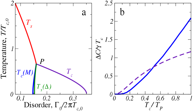
Figure 3: (Color online) a) The phase diagram as a function of disorder, $\Gamma_{0}/2\pi T_{c,0}$ for $\Gamma_{\pi}=0.2\Gamma_{0}$ and $T_{s,0}/T_{c,0}=3$. Note that the region of the mixed phases gets narrower than the region for on-cite impurities, cf. 1. b) The specific heat jump as a function of $T_{c}/T_{P}$. The solid line represents the specific heat jump ${\mbox{\footnotesize$\Delta$}}C/T_{c}$ for normal–to–SC transition, and the dashed line shows ${\mbox{\footnotesize$\Delta$}}C/T_{c}$ in the overdoped region for transition between SDW and SC coexistence phases.

The behavior of ${\mbox{\footnotesize$\Delta$}}C/T_{c}$ as a function of doping–induced disorder is shown in Figs. 1b, 2, and 3b. To evaluate ${\mbox{\footnotesize$\Delta$}}C/T_{c}$ at the transition from a normal metal to a superconductor above optimal doping we use Eqs. (38) for $\alpha^{\prime}$ and $\beta$ in Eq. (41). At large doping, when $T_{c}$ is significantly suppressed and the system enters the regime of impurity–induced gapless superconductivity, specific heat jump ${\mbox{\footnotesize$\Delta$}}C/T_{c}$ decreases with $T_{c}$ as ${\mbox{\footnotesize$\Delta$}}C/T_{c}\propto T^{2}_{c}$, Ref. Kogan, 2009. Away from the gapless regime, the dependence of ${\mbox{\footnotesize$\Delta$}}C/T_{c}$ on $T_{c}$ is more complex and differs from $T^{2}_{c}$, as the dashed lines in Figs.  1b, 2, and 3b. For completeness we present in Fig. 4 ${\mbox{\footnotesize$\Delta$}}C/T_{c}$ as a function of $T_{c}/T_{c,0}$ for an $s^{\pm}$ superconductor, when there is no competing SDW instability (i.e., when $\lambda_{\rm sdw}=0$) and the $T_{c}$ line extends to $T_{c,0}$ in the clean limit.

For the transition from the preexisting SDW state into the mixed state below optimal doping, we compute ${\mbox{\footnotesize$\Delta$}}C/T_{c}$, Eq. (41), using $\alpha^{\prime}$ and $\beta$ from Eqs. (27) and (37). In this regime, SDW order strengthen as doping decreases, and SDW correlations suppress both superconducting $T_{c}(M)$ and ${\mbox{\footnotesize$\Delta$}}C/T_{c}$. In particular, the rapid decrease of ${\mbox{\footnotesize$\Delta$}}C/T_{c}$ at smaller dopings is an indicator that fewer quasiparticle states participate in superconducting pairing, as the low-energy states are pushed away from the FS by SDW order. We see therefore that ${\mbox{\footnotesize$\Delta$}}C/T_{c}$ drops at deviations from optimal doping in both overdopped and underdopped regimes.

It is essential that in the disorder model, the behavior of ${\mbox{\footnotesize$\Delta$}}C/T_{c}$ in the underdoped and overdoped regimes is governed by the single parameter $\Gamma_{0}\propto n_{imp}$, assuming that the ratio $\Gamma_{\pi}/\Gamma_{0}$ is kept constant. The same parameter $\Gamma_{0}$ also defines $T_{c}/T_{P}$, where $T_{P}=T_{c}(M\to 0)$ is the transition temperature at the tetracritical point. One can therefore make a direct comparison with experiments by plotting ${\mbox{\footnotesize$\Delta$}}C/T_{c}$ above and below optimal doping as the function of the same $T_{c}/T_{P}$ using ${\mbox{\footnotesize$\Delta$}}C$ defined by Eq. (41) with $\alpha^{\prime}$ and $\beta$ given by Eqs. (38) above optimal doping, and by Eqs. (27) and (37) for a finite $M$ below optimal doping. Experiments show Bud’ko et al. (2009); Hardy et al. (2010a, b) that ${\mbox{\footnotesize$\Delta$}}C/T_{c}$ drops faster in underdoped regime, but in log-log plot the data from underdoped and overdoped regimes can be reasonably well fitted by a quadratic law ${\mbox{\footnotesize$\Delta$}}C/T_{c}\propto T_{c}^{2}$.

We plot our ${\mbox{\footnotesize$\Delta$}}C/T_{c}$ in Fig. 2 as functions of $T_{c}/T_{P}$ in both linear and log-log plots. We see that ${\mbox{\footnotesize$\Delta$}}C/T_{c}$ drops faster with decreasing $T_{c}$ in the underdoped regime, i.e. in the mixed phase. This behavior is consistent with experimental data. The $T$ dependence of ${\mbox{\footnotesize$\Delta$}}C/T_{c}$ is not exactly $T^{2}$ , but looks reasonably close to $T^{2}$ in log-log plot (right panel in Fig. 2), although such plot puts more weight on the data at low $T_{c}$ where the $T-$dependence of ${\mbox{\footnotesize$\Delta$}}C/T_{c}$ is the strongest.

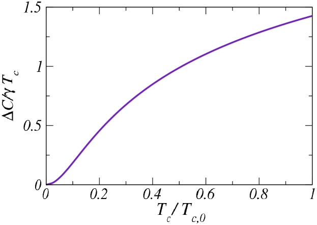
Figure 4: (Color online) The jump ${\mbox{\footnotesize$\Delta$}}C/T_{c}$ of the specific heat at a superconducting $T_{c}$ without a competing SDW instability ($\lambda_{\rm sdw}=0$). ${\mbox{\footnotesize$\Delta$}}C/T_{c}$ is plotted as a function of $T_{c}/T_{c,0}$, where $T_{c,0}$ is the superconducting transition temperature in the clean limit.

Finally, we note that ${\mbox{\footnotesize$\Delta$}}C/T_{c}$ is discontinuous at the tetra-critical point $T_{c}=T_{s}=T_{P}$. The discontinuity is the manifestation of the discontinuous change in both $\alpha^{\prime}$ and $\beta$ across $T_{P}$. The discontinuity in $\alpha^{\prime}$ is due to the fact that the second term in (27) is zero for $M=0$, but is finite when $M\neq 0$ and contains temperature derivative of $(g^{(0)}_{\omega_{n}}-1)\propto M^{2}\propto(T-T_{P})$. The discontinuity in $\beta$ is due to the feedback term $C^{2}/B$ in $\beta$, which remains finite upon approaching $T_{P}$ from smaller dopings, but is absent in the overdoped regime, where $T_{s}<T_{c}$. The interplay between discontinuities in $\alpha^{\prime}$ and $\beta$ in the disorder model is such that ${\mbox{\footnotesize$\Delta$}}C/T_{c}$ jumps up at $n_{\rm imp}$ once the system enters the mixed phase.

The discontinuity in ${\mbox{\footnotesize$\Delta$}}C/T_{c}$ at $T_{P}$ has also been found in the rigid band model.Vavilov et al. (2011) In that model, however, the magnitude and the sign of the jump in ${\mbox{\footnotesize$\Delta$}}C/T_{c}$ depend on the FS geometry and ${\mbox{\footnotesize$\Delta$}}C/T_{c}$ may actually drop down upon entering into the mixed phase. We also emphasize that discontinuity in ${\mbox{\footnotesize$\Delta$}}C/T_{c}$ only holds within the mean–field theory and gets rounded up and transforms into a maximum once we include fluctuations because then the thermodynamic average $\langle M^{2}\rangle$ is non-zero on both sides of the tetra-critical point. This behavior of ${\mbox{\footnotesize$\Delta$}}C/T_{c}$ in the presence of fluctuations is schematically illustrated in Fig. 1b by the dashed line.

VI Conclusions

In this paper we obtained the phase diagram of doped Fe-pnictides and the specific heat jump ${\mbox{\footnotesize$\Delta$}}C$ at the onset of superconductivity across the phase diagram under the assumption that doping introduces disorder but does not affect the band structure. The phase diagram is quite similar to the one obtained in the rigid band scenario and contains SDW and SC phases and the region where SDW and SC orders co-exist. The ratio ${\mbox{\footnotesize$\Delta$}}C/T_{c}$, which is a constant in a BCS superconductor, is non-monotonic across the phase diagram – it has a maximum at the tetra-critical point at the onset of the mixed phase and drops at both larger and smaller dopings. The behavior at large and small dopings is described in terms of the single parameter: the impurity density $n_{\rm imp}$. The non-monotonic behavior of ${\mbox{\footnotesize$\Delta$}}C/T_{c}$ in the underdoped regime also holds in the rigid band model,Vavilov et al. (2011) but there the behavior of ${\mbox{\footnotesize$\Delta$}}C/T_{c}$ at small and large dopings is generally uncorrelated.

We found reasonably good agreement between our theory and the experimental phase diagram of Ba(Fe_1-xRu_x)₂As₂, in which Fe is subsituted by isovalent $Ru$ (see Refs.Brouet et al. (2010); Dhaka et al. (2011)) and on the data for the doping dependence of the specific heat jump at $T_{c}$. Bud’ko et al. (2009); Hardy et al. (2010a, b) This agreement is a good indicator that our theory captures the key physics of non-monotonic behavior of ${\mbox{\footnotesize$\Delta$}}C/T_{c}$, particularly the reduction of ${\mbox{\footnotesize$\Delta$}}C/T_{c}$ in the mixed state. Whether the data can distinguish between rigid band and disorder scenarios is a more subtle issue as the interplay between doping-induced disorder and doping-induced change in the band structure is likely to be material-dependent. Another subtle issue is the apparent $T^{2}$ dependence of the measured ${\mbox{\footnotesize$\Delta$}}C/T_{c}$ on both sides of optimal doping. Our log-log plots reproduce this dependence reasonably well, but our actual ${\mbox{\footnotesize$\Delta$}}C/T_{c}$ are more mild than $T^{2}$. One possible reason is our neglect of the doping dependence of $\gamma$ in the normal state specific heat $C=\gamma T$. In reality, $\gamma$ also decreases on both sides of optimal doping,Hardy et al. (2010a) and this should sharpen up the $T$ dependence of ${\mbox{\footnotesize$\Delta$}}C/T_{c}$.

Finally, there are certainly other elements of the physics of Ba(Fe_1-xRu_x)₂As₂ which we neglected in our model. In particular, Brouet et al. demonstrated Brouet et al. (2010) that Fermi velocities in Ba(Fe_1-xRu_x)₂As₂ are larger than in undoped BaFe₂As₂, this observation likely implies that electronic correlations are weaker in Ba(Fe_1-xRu_x)₂As₂. Dhaka et al. arguedDhaka et al. (2011) that magnetic dilution due to Ru substitution contributes to the destruction of SDW order. These effects add on top of Ru-induced impurity scattering, which we studied here, and call for more comprehensive analysis of isolvalent doping of Fe in 122 materials.

References

• Hirschfeld et al. (2011) P. Hirschfeld, M. Korshunov, and I. Mazin (2011), eprint 1106.3712v1.
• Wadati et al. (2010) H. Wadati, I. Elfimov, and G. A. Sawatzky, Phys. Rev. Lett. 105, 157004 (2010).
• Fernandes et al. (2010) R. M. Fernandes, D. K. Pratt, W. Tian, J. Zarestky, A. Kreyssig, S. Nandi, M. G. Kim, A. Thaler, N. Ni, P. C. Canfield, et al., Phys. Rev. B 81, 140501 (2010).
• Vorontsov et al. (2009) A. B. Vorontsov, M. G. Vavilov, and A. V. Chubukov, Phys. Rev. B 79, 060508 (2009).
• Cvetkovic and Tesanovic (2009) V. Cvetkovic and Z. Tesanovic, EPL 85, 37002 (2009).
• Brouet et al. (2010) V. Brouet, F. Rullier-Albenque, M. Marsi, B. Mansart, M. Aichhorn, S. Biermann, J. Faure, L. Perfetti, A. Taleb-Ibrahimi, P. Le Fèvre, et al., Phys. Rev. Lett. 105, 087001 (2010).
• Dhaka et al. (2011) R. S. Dhaka, C. Liu, R. M. Fernandes, R. Jiang, C. P. Strehlow, T. Kondo, A. Thaler, J. Schmalian, S. L. Bud’ko, P. C. Canfield, et al. (2011), eprint arXiv:1108.0711v1.
• Kaminski. (2011) A. Kaminski., Private communication (2011).
• Tarantini et al. (2010) C. Tarantini, M. Putti, et al., Phys. Rev. Lett. 104, 087002 (2010).
• Kim et al. (2010) H. Kim, R. T. Gordon, et al., Phys. Rev. B 82, 060518 (2010).
• (11) N. I. Kulikov and V. V. Tugushev, Usp. Fiz. Nauk 144, 643 (1984) [Sov. Phys. Usp. 27, 954 (1984)].
• Dolgov et al. (2009) O. V. Dolgov, A. A. Golubov, and D. Parker, New Journal of Physics 11, 075012 (2009).
• Vorontsov et al. (2009) A. B. Vorontsov, M. G. Vavilov, and A. V. Chubukov, Phys. Rev. B 79, 140507 (2009).
• Bang (2009) Y. Bang, EPL (Europhysics Letters) 86, 47001 (2009).
• Bud’ko et al. (2009) S. L. Bud’ko, N. Ni, and P. C. Canfield, Phys. Rev. B 79, 220516 (2009).
• Hardy et al. (2010a) F. Hardy, T. Wolf, R. A. Fisher, R. Eder, P. Schweiss, P. Adelmann, H. v. Löhneysen, and C. Meingast, Phys. Rev. B 81, 060501 (2010a).
• Hardy et al. (2010b) F. Hardy, P. Burger, et al., EPL (Europhysics Letters) 91, 47008 (2010b).
• Wang et al. (2008) Z.-S. Wang, H.-Q. Luo, C. Ren, and H.-H. Wen, Phys. Rev. B 78, 140501 (2008).
• Vavilov et al. (2011) M. G. Vavilov, A. V. Chubukov, and A. B. Vorontsov, Phys. Rev. B 84, 140502(R) (2011).
• Chubukov et al. (2008) A. V. Chubukov, D. V. Efremov, and I. Eremin, Phys. Rev. B 78, 134512 (2008).
• Maiti and Chubukov (2010) S. Maiti and A. V. Chubukov, Phys. Rev. B 82, 214515 (2010).
• Wang et al. (2009) F. Wang, H. Zhai, Y. Ran, A. Vishwanath, and D.-H. Lee, Phys. Rev. Lett. 102, 047005 (2009).
• Thomale et al. (2009) R. Thomale, C. Platt, J. Hu, C. Honerkamp, and B. A. Bernevig, Phys. Rev. B 80, 180505 (2009).
• Platt et al. (2009) C. Platt, C. Honerkamp, and W. Hanke, New Journal of Physics 11, 055058 (2009).
• Eilenberger (1968) G. Eilenberger, Zeitschrift for Physik 214, 195 (1968).
• Moor et al. (2011) A. Moor, A. F. Volkov, and K. B. Efetov, Phys. Rev. B 83, 134524 (2011).
• Abrikosov and Gorkov (1961) A. A. Abrikosov and L. P. Gorkov, ZhETF, 39 1781 (1960) [Sov. Phys. JETP 12, 1243 (1961)].
• Balatsky et al. (2006) A. V. Balatsky, I. Vekhter, and J.-X. Zhu, Rev. Mod. Phys. 78, 373 (2006).
• Galitski (2008) V. Galitski, Phys. Rev. B 77, 100502 (2008).
• Vorontsov et al. (2010) A. B. Vorontsov, A. Abanov, M. G. Vavilov, and A. V. Chubukov, Phys. Rev. B 81, 012508 (2010).
• Moon and Sachdev (2010) E. G. Moon and S. Sachdev, Phys. Rev. B 82, 104516 (2010).
• (32) A. A. Abrikosov, L. P. Gorkov, and I. E. Dzyaloshinski, Methods of quantum field theory in statistical physics, (Dover Publications, New York, 1963); E. M. Lifshitz and L. P. Pitaevski, Statistical Physics, (Pergamon Press, 1980).
• Kogan (2009) V. G. Kogan, Phys. Rev. B 80, 214532 (2009).