Infinite family of second-law-like inequalities

Abstract

The probability distribution function for an out of equilibrium system may sometimes be approximated by a physically motivated “trial” distribution. A particularly interesting case is when a driven system (e.g., active matter) is approximated by a thermodynamic one. We show here that every set of trial distributions yields an inequality playing the role of a generalization of the second law. The better the approximation is, the more constraining the inequality becomes: this suggests a criterion for its accuracy, as well as an optimization procedure that may be implemented numerically and even experimentally. The fluctuation relation behind this inequality, -a natural and practical extension of the Hatano-Sasa theorem-, does not rely on the a priori knowledge of the stationary probability distribution.

I Introduction

A recurring strategy applied to out of equilibrium systems is to represent the complex energy and dissipation sources by a bath with good equilibrium thermal properties. Two examples are the Edwards “thermodynamic“ approach to granular matter edw and recent developments for active matter (see Refs. jor ; leticia ; wolynes for recent examples), in which the combination of rapid energy bursts and friction is mimicked by a thermal bath. The aim of such pursuits is not necessarily to make the problem more easily solvable, but rather to cast it in a form that provides thermodynamic intuition and constraints. In this paper we derive some simple relations that help make this mapping more systematic and controlled. The method is based on the use of inequalities of the form of the second law, associated with each guess for the distribution function.

In these last two decades there has been a development of a family of relations valid for out of equilibrium systems reviews , including the fluctuation theorem in its various forms EvCoMo ; GaCo ; Ku ; Hurtado and the Jarzynski Ja and Crooks Cr relations. A later and extremely simple result is the Hatano-Sasa equality HaSa , which applies to systems that are continuously driven by time-dependent potentials inducing currents, so that even the stationary regimes are out of equilibrium. Their result is essentially a version of Jarzynski equality and the second principle, but with the energy replaced by the logarithm of the stationary distribution.

In this paper we derive an extension of the Hatano-Sasa theorem for Markovian systems, which has the practical advantage that it does not rely on the a priori knowledge of the stationary probability distribution. Instead, arbitrary “trial” smooth distributions can be used, thus allowing one to treat systems whose stationary distribution is either (i) too difficult to calculate, as generically occurs in out of equilibrium systems with many degrees of freedom, or (ii) unwieldy, as, for instance, in the deterministic limit, where the nonequilibrium steady-state distributions are nonzero only over a fractal support. Our approach leads in particular to an inequality that can be used as a variational principle for improving, in a controlled way, physically motivated approximations to nonequilibrium steady-state distributions. The optimization procedure might be implemented numerically or even experimentally. As an illustration, we numerically approximate the stationary distribution of a paradigmatic non-equilibrium driven system with many degrees of freedom, the simple symmetric exclusion process in one dimension.

Just as in the case of the Hatano-Sasa equality HaSa ; Esposito , there is a “dual” (or adjoint) “backward” process that yields, when compared to the forward process of the original dynamics, a trajectory-dependent quantity playing the role of an entropy production that satisfies a form of the fluctuation theorem. For systems described by a Langevin dynamics, the dual backward process is obtained easily since it is given by a Langevin dynamics involving only additional a priori known external forces derived from the trial function itself. This remarkable property offers the possibility to explore numerically or even experimentally the interesting consequences of the associated detailed fluctuation relations, valid for systems that spontaneously relax to nonequilibrium steady states.

The organization of this paper is as follows. In Sec. II we review the derivation of the Hatano-Sasa fluctuation theorem  HaSa . After motivating a more general approach we provide in Sec. III.1 a first derivation of the integral version of our fluctuation relation along the same lines of the original Hatano-Sasa derivation. In Sec. III.2 we give a second, more general derivation, which yields the detailed version of the theorem (containing the integral version as a particular case), and in Sec. III.3 we discuss the physical interpretation of the dual dynamics behind it. In Sec. III.4 we discuss a family of inequalities that plays the role of the second law. In Sec. IV we propose an optimization procedure for approximating steady-state distributions. As an example, we apply it to the paradigmatic symmetric exclusion process in one dimension. In Sec. V we give a conclusion and perspectives.

II The Hatano-Sasa relation

Consider a driven system with dynamic variables ${\bf x}$ with time-dependent external fields $\alpha(t)$ (e.g., shear rate, temperature gradient, etc.), with distribution $\rho({\bf x},t)$ evolving through a generator $H(\alpha)$:

$${\dot{\rho}({\bf x},t)=-H(\alpha(t))\;\rho({\bf x},t)}.$$ (1)

Let us assume the dynamics admit, for every fixed value of the parameter $\alpha$, a nonequilibrium steady state with distribution

$${\rho_{ss}({\bf x};\alpha)=e^{-\phi({\bf{x}};\alpha)}}\;\;\;\;\;\;\;\;;\;\;\;\;\;\;\;\;H(\alpha)\rho_{ss}({\bf x};\alpha)=0.$$ (2)

The Hatano-Sasa HaSa result may be written

$$\left\langle e^{-\int_{0}^{\tau}dt\;\frac{\partial\phi({\bf{x}};\alpha)}{\partial\alpha}{\dot{\alpha}}}\right\rangle_{\rho_{ss}({\bf{x}};\alpha_{1})}=1,$$ (3)

which implies, by virtue of Jensen’s inequality,

$${\left\langle\int_{\alpha_{1}}^{\alpha(\tau)}\frac{\partial\phi({\bf{x}};\alpha)}{\partial\alpha}d{\alpha}\right\rangle_{\rho_{ss}({\bf{x}};\alpha_{1})}\geq 0.}$$ (4)

The average $\langle\bullet\rangle$ is over all trajectories ${\bf x}(t)$ of duration $\tau$, starting with an initial configuration chosen with the distribution $\rho_{ss}({\bf{x}};\alpha_{1})$ with $\alpha_{1}\equiv\alpha(0)$. We shall refer to (3) and (4) as the Hatano-Sasa equality and inequality, respectively. In the particular case in which the stationary states $\rho_{ss}({\bf{x}};\alpha)$ are Gibbs states we have

$$\rho_{ss}({\bf x};\alpha)=\frac{e^{-\beta E({\bf x},\alpha)}}{e^{-\beta F(\alpha)}};\phi({\bf{x}};\alpha)=\beta[E({\bf x},\alpha)-F(\alpha)]$$ (5)

and the Hatano-Sasa equality and inequality become the Jarzynski equality and the second law, respectively.

The proof is extremely simple. We start by decomposing the evolution in a large number $M$ of time steps and compute, in operator (bra-ket) formalism, the quantity

$$\langle -|e^{-\frac{\tau}{M}H(\alpha_{M})}\frac{\hat{\rho}_{ss}(\alpha_{M})}{\hat{\rho}_{ss}(\alpha_{M-1})}...\frac{\hat{\rho}_{ss}(\alpha_{3})}{\hat{\rho}_{ss}(\alpha_{2})}e^{-\frac{\tau}{M}H(\alpha_{2})}$$ (6)

$$\frac{\hat{\rho}_{ss}(\alpha_{2})}{\hat{\rho}_{ss}(\alpha_{1})}e^{-\frac{\tau}{M}H(\alpha_{1})}|\rho_{ss}(\alpha_{1})\rangle=\langle-|\rho_{ss}(\alpha_{M})\rangle=1,$$

where $e^{-\frac{\tau}{M}H(\alpha_{i})}|\rho_{ss}(\alpha_{i})\rangle=|\rho_{ss}(\alpha_{i+1})\rangle$. We denote $\hat{\rho}(\alpha)$ as the operator such that $\langle{\bf x}|\hat{\rho}(\alpha)|{\bf x^{\prime}}\rangle=\delta({\bf x}-{\bf x^{\prime}})\;\rho({\bf x};\alpha)$ and $|\rho(\alpha)\rangle$ as the state such that $\rho({\bf x};\alpha)\equiv\langle{\bf x}|\rho(\alpha)\rangle$. The state $|-\rangle$ corresponds to the flat distribution $\langle{\bf x}|-\rangle=1$; i.e., the left eigenvector of $H(\alpha)$ has zero eigenvalue.

Now, using that the time step $\tau/M$ is small, we can write

$$\frac{{\rho}_{ss}({\bf x};\alpha_{k+1})}{{\rho}_{ss}({\bf x};\alpha_{k})}\approx e^{-\frac{\tau}{M}\;\;\frac{\partial{\phi}({\bf{x}};\alpha_{k})}{\partial\alpha}\;{\dot{\alpha}}}.$$ (7)

Therefore (6) may be written as Eq. (3), and the result is proven. The exponential of the term $\left[-\int dt\;\frac{\partial\phi({\bf x};\alpha)}{\partial\alpha}\;{\dot{\alpha}}\right]$, a functional of the trajectory, is thus weighted in (3) with the probability of each dynamical trajectory ${\bf x}(t)$ such that ${\bf x}(0)$ is sampled from $\rho_{ss}({\bf x},\alpha_{1})$.

In the Hatano-Sasa inequality (4), the equality holds in the quasistationary limit, when the probability distribution may be assumed to be, at each time $t$, the stationary one $\rho_{ss}({\bf x};\alpha)$ corresponding to the value of $\alpha$ at that time:

$$\left\langle\int\frac{\partial\phi({\bf{x}};\alpha)}{\partial\alpha}d\alpha\right\rangle=\int d{\bf{x}}\;d\alpha\;e^{-\phi({\bf{x}};\alpha)}\frac{\partial\phi({\bf{x}};\alpha)}{\partial\alpha}$$ (8)

$$= \int d{\bf{x}}[\rho_{ss}({\bf{x}};\alpha_{M})-\rho_{ss}({\bf{x}};\alpha_{1})]=0.$$

This result is the generalization of the entropy change ${S}(\alpha_{M})-{S}(\alpha_{1})=\langle\int_{0}^{\tau}dt\;\dot{{\bf{x}}}\cdot\nabla\phi\rangle$, under reversible transformations, with ${S}(\alpha)\equiv-\int d{\bf x}\rho_{ss}({\bf x};\alpha)\ln\rho_{ss}({\bf x};\alpha)$ being the generalized Shannon entropy HaSa .

III A more general approach

The quantity $\phi({\bf x};\alpha)=-\ln\rho_{ss}({\bf x};\alpha)$ plays a role similar to the one of the energy function in a system with detailed balance, but it may become intractable as soon as we consider a driven system. The first difficulty is that it is, in general, impossible to obtain analytically. This is aggravated by the fact that in order to use (3) and (4), we need to know $\rho_{ss}$ also where it is exponentially small. Another more serious problem arises from the fact that the function $\phi({\bf x};\alpha)$ may only be small in a limited domain and very large everywhere else. An extreme form of this situation arises in the deterministic limit. Consider a noisy dynamics with a (Hoover Hoover ) thermostat:

$$\left\{\begin{array}[]{ll}\dot{q}_{i}&={p_{i}},\\ {}\\ \dot{p}_{i}&=-\frac{\partial{\mathcal{H}}}{\partial q_{i}}+\underbrace{\gamma(t)p_{i}}_{\text{thermostat}}{-\underbrace{f_{i}({\bf q})}_{\text{forcing}}-\underbrace{\bf\eta_{i}(t)}_{\text{noise}}},\end{array}\right.$$ (9)

where ${\bf\eta(t)}$ is a Gaussian white noise of variance $\epsilon$. Energy is conserved provided $\gamma(t)=\frac{{\bf(f+{\bm{\eta}})}\cdot{\bf p}}{{\bf p^{2}}}$. When there is forcing ${\bf f}\neq 0$, the stationary distribution is not flat. Indeed, in the limit of zero noise $\epsilon\to 0$, $\rho_{ss}$ has, in fact, fractal support, and $\phi({\bf x};\alpha)$ is infinity almost everywhere on the energy surface. If we attempt to apply the Hatano-Sasa inequality for a small noise amplitude in a process with varying $\alpha$, because the region on the energy shell where $\phi({\bf x};\alpha)$ is small is sparse and strongly dependent on $\alpha$, almost all of the process takes place in regions in which $\phi({\bf x};\alpha)$ is large: the trajectories are very far from quasistationary, and the Hatano-Sasa inequality, though true, becomes useless.

A similar situation arises when the potential is rapidly oscillating, as in vibrated granular matter, which we may think of as subjected to an oscillating gravity field. Here again, the system is always very far from the stationary situation corresponding to any instantaneous value of the field because it does not have the time to catch up with the oscillating stationary measure. And yet we still observe that rapidly vibrated granular matter behaves in a manner that resembles motion in contact with a heat bath and would expect some form of second law to apply in that case.

With the above motivations, we look for a more flexible approach. Instead of working with the true stationary distributions $\rho_{ss}({\bf x};\alpha)$, we choose an arbitrary family of smooth functions as reference states ${\rho_{\tt ref}}({\bf x};\alpha)$ and the corresponding ${\phi_{\tt ref}}({\bf x};\alpha)\equiv-\ln{\rho_{\tt ref}}({\bf x};\alpha)$. In the following we derive an extension of the Hatano-Sasa integral and detailed fluctuation relations, using only these smooth functions.

III.1 Integral fluctuation theorem

In order to obtain a relation, we go through the same steps as in Sec. II. Starting from the initial distribution ${\phi_{\tt ref}}({\bf x};\alpha_{1})$, we compute, just as in (6),

$$\langle - |e^{-\frac{\tau}{M}H(\alpha_{M})}\frac{\hat{\rho}_{\tt ref}(\alpha_{M})}{\tilde{\rho}_{\tt ref}(\alpha_{M-1})}...\frac{\hat{\rho}_{\tt ref}(\alpha_{2})}{\tilde{\rho}_{\tt ref}(\alpha_{1})}e^{-\frac{\tau}{M}H(\alpha_{1})}|{\rho_{\tt ref}}(\alpha_{1})\rangle$$ (10)

$$= \langle-|{\rho_{\tt ref}}(\alpha_{M})\rangle=1,$$

but with $\tilde{\rho}(\alpha)$ being the operator associated with the state evolved by one time step $e^{-\frac{\tau}{M}H(\alpha)}|\rho(\alpha)\rangle$. We can thus write, for large $M$,

$$\frac{\tilde{\rho}_{\tt ref}({\bf x};\alpha)}{{\rho}_{\tt ref}({\bf x};\alpha)}\approx e^{\frac{\tau}{M}{\varphi}({\bf x};\alpha)},$$ (11)

with

$$\varphi({\bf{x}};\alpha)\equiv-\frac{1}{{\rho_{\tt ref}}({\bf{x}};\alpha)}\;\{H(\alpha)\;{\rho_{\tt ref}}({\bf{x}};\alpha)\}.$$ (12)

Here $H(\alpha)$ acts over the function ${\rho_{\tt ref}}({\bf{x}};\alpha)$, so that it is in fact $\varphi({\bf{x}};\alpha)=-\langle{\bf{x}}|\frac{1}{\hat{\rho}_{\tt ref}(\alpha)}H(\alpha)|{\rho_{\tt ref}}(\alpha)\rangle$. We hence have

$$\frac{{\rho_{\tt ref}}({\bf x};\alpha_{k+1})}{\tilde{\rho}_{\tt ref}({\bf x};\alpha_{k})}\approx e^{-\frac{\tau}{M}\;\;\frac{\partial{\phi_{\tt ref}}({\bf{x}};\alpha_{k})}{\partial\alpha}\;{\dot{\alpha}}-\frac{\tau}{M}\;{\varphi(\bf x,\alpha)}},$$ (13)

and we obtain a new equality, valid for all sets ${\phi_{\tt ref}}({\bf{x}};\alpha)$,

$$\left\langle e^{-\int dt\;\frac{\partial{\phi_{\tt ref}}({\bf{x}};\alpha)}{\partial\alpha}\;{\dot{\alpha}}\;\;{-\int dt\;\varphi({\bf x};\alpha)}}\right\rangle_{{\rho_{\tt ref}}({\bf{x}};\alpha_{1})}=1,$$ (14)

which is the first main result of our paper. Defining

$${\mathcal{Y}}\equiv\int dt\;\frac{\partial{\phi_{\tt ref}}({\bf{x}};\alpha)}{\partial\alpha}\;{\dot{\alpha}}\;\;{+\int dt\;\varphi({\bf x};\alpha)}$$ (15)

it can be simply written as $\langle e^{-{\mathcal{Y}}}\rangle=1$. This integral fluctuation theorem is valid for any protocol $\alpha(t)$ and arbitrary times $\tau$, like the Hatano-Sasa equality, to which it reduces if the reference state is chosen as ${\rho_{\tt ref}}({\bf x};\alpha)=\rho_{ss}({\bf x};\alpha)$, but it holds for arbitrary smooth functions ${\rho_{\tt ref}}$ Sag .

As we shall see, this immediately implies an inequality $\langle{\mathcal{Y}}\rangle\geq 0$ of the form of the second law.

III.2 Detailed fluctuation theorem

Just as in the case of the Hatano-Sasa relation, the result of Eq. (14) can be alternatively derived as a particular case of a detailed fluctuation theorem. We will use here a procedure that generalizes the one used for obtaining the detailed fluctuation theorem associated with the Hatano-Sasa theorem HaSa ; chernyak ; Esposito ; Reinaldo .

We are looking for a time-reversed form of the dynamics. Let us start by rewriting (10) as

$$\langle - |e^{-\frac{\tau}{M}H(\alpha_{M})}\frac{\hat{\rho}_{\tt ref}(\alpha_{M})}{\tilde{\rho}_{\tt ref}(\alpha_{M-1})}...\frac{\hat{\rho}_{\tt ref}(\alpha_{2})}{\tilde{\rho}_{\tt ref}(\alpha_{1})}e^{-\frac{\tau}{M}H(\alpha_{1})}|{\rho_{\tt ref}}(\alpha_{1})\rangle$$

$$= \langle{\rho}_{\tt ref}(\alpha_{M})|\frac{1}{\tilde{\rho}_{\tt ref}(\alpha_{M-1})}...\frac{\hat{\rho}_{\tt ref}(\alpha_{2})}{\tilde{\rho}_{\tt ref}(\alpha_{1})}e^{-\frac{\tau}{M}H(\alpha_{1})}{\hat{\rho}}_{\tt ref}(\alpha_{1})|-\rangle$$

$$= \langle{\rho}_{\tt ref}(\alpha_{M})|\Pi_{k=1}^{M-1}\left[\frac{1}{\tilde{\rho}_{\tt ref}(\alpha_{k})}e^{-\frac{\tau}{M}H(\alpha_{k})}{\hat{\rho}}_{\tt ref}(\alpha_{k})\right]|-\rangle.$$

We may now take the adjoint in order to reverse time:

$$\langle -|\Pi_{k=M-1}^{1}\left[\frac{1}{\tilde{\rho}_{\tt ref}(\alpha_{k})}e^{-\frac{\tau}{M}H(\alpha_{k})}{\hat{\rho}}_{\tt ref}(\alpha_{k})\right]^{\dagger}|{\rho}_{\tt ref}(\alpha_{M})\rangle=$$

$$\langle- | \Pi_{k=M-1}^{1}\left[\frac{1}{\hat{\rho}_{\tt ref}(\alpha_{k})}e^{-\frac{\tau}{M}\{H(\alpha_{k})+\varphi(\alpha_{k})\}}{\hat{\rho}}_{\tt ref}(\alpha_{k})\right]^{\dagger}|{\rho}_{\tt ref}(\alpha_{M})\rangle$$

$$= \langle-|\Pi_{k=M-1}^{1}\left[e^{-\frac{\tau}{M}H^{adj}(\alpha_{k})}\right]|{\rho}_{\tt ref}(\alpha_{M})\rangle.$$

This is a time-reversed dynamics with generator:

$$[H^{adj}(\alpha)]^{{\dagger}}\equiv\frac{1}{{\hat{\rho}}_{\tt ref}(\alpha)}\;\{H(\alpha)+\varphi(\alpha)\}\;{\hat{\rho}}_{\tt ref}(\alpha).$$ (16)

We shall see below that it corresponds, in fact, to a Langevin process with a modified force field [see Eq. (27)].

In terms of the original and the adjoint dynamics, the evolution in time step $\tau/M$ is

$$P({\bf x}^{\prime}|{\bf x};\alpha)\equiv\langle{\bf x}^{\prime}|e^{-\frac{\tau}{M}{H}_{\alpha}}|{\bf x}\rangle,$$ (17)

$${P^{adj}}({\bf x}^{\prime}|{\bf x};\alpha)\equiv\langle{\bf x}^{\prime}|e^{-\frac{\tau}{M}{H}^{adj}_{\alpha}}|{\bf x}\rangle.$$ (18)

The construction (16) tells us that , for each trajectory $\mathcal{T}\equiv\{{\bf x}_{1},{\bf x}_{2},...,{\bf x}_{M}\}$ with the initial condition chosen with probability $\rho_{\tt ref}({\bf x}_{1};\alpha_{1})$, there is a time-reversed ($R$) trajectory, with the initial condition chosen with probability $\rho_{\tt ref}({\bf x}_{M};\alpha_{M})$, and their respective weights are

$$\mathcal{P}[\mathcal{T};\alpha] = \prod_{n=1}^{M-1}P({\bf x}_{n+1}|{\bf x}_{n};\alpha_{n})\rho_{\tt ref}({\bf x}_{1};\alpha_{1}),$$

and

$$\left[{\mathcal{P}^{{adj}}}[\mathcal{T};\alpha]\right]^{R} = \prod_{n=1}^{M-1}{P^{adj}}({\bf x}_{n}|{\bf x}_{n+1};\alpha_{n})\rho_{\tt ref}({\bf x}_{M};\alpha_{M}).$$

We thus may define a quantity $\Xi[\mathcal{T};\alpha]$ associated with each path, having an interpretation analogous to the entropy production,

$$\Xi[\mathcal{T};\alpha]\equiv\ln\frac{\mathcal{P}[\mathcal{T},\alpha]}{\left[\mathcal{P}^{{adj}}[\mathcal{T},\alpha]\right]^{R}}.$$ (19)

In the large $M$ limit, it becomes

$$\Xi[\mathcal{T};\alpha]\approx\int_{0}^{\tau}dt\;\left[{\varphi}({\bf x};\alpha)+\dot{\alpha}\partial_{\alpha}\phi_{\tt ref}({\bf x},\alpha)\right].$$ (20)

It is clear from Eq. (19) that, in terms of $\Xi$, there is a detailed fluctuation theorem:

$$\langle\mathcal{O}[\mathcal{T}]e^{-\Xi[\mathcal{T},\alpha]}\rangle = \langle\mathcal{O}[\mathcal{T}]e^{-\int_{0}^{\tau}dt\;\left[\varphi({\bf x};\alpha)+\dot{\alpha}\partial_{\alpha}{\phi_{\tt ref}}({\bf x},\alpha)\right]}\rangle$$ (21)

$$= {\left[{\langle\mathcal{O}[\mathcal{T}]\rangle}^{{adj}}\right]^{R}},$$

which is valid for an arbitrary functional $\mathcal{O}[\mathcal{T}]$ of the trajectory. The averages in (21) are performed with the real forward dynamics in the first term and with the time-reversed adjoint dynamics of Eq. (18) in the second term.

Equation (21) is a very general result. It represents a broad family of fluctuation theorems with a trajectory dependent “entropy production” of the form of Eq. (20), completely determined by the distributions $\rho_{\tt ref}({\bf{x}};\alpha)$.

Clearly, choosing $\mathcal{O}=1$ in this equation we get the integral fluctuation relation of Eq. (14). This detailed fluctuation theorem, which can be used to derive a variety of Crooks-like relations, is the second main result of our paper.

III.3 Generalized dual (adjoint) dynamics

In order to give a simple physical interpretation of the dual dynamics let us now assume that our system is governed by a Langevin equation,

$$\dot{{\bf x}}={\bf f}({\bf x};\alpha)+{\bm{\xi}}(t),$$ (22)

with ${\bf f}({\bf x};\alpha)$ being an arbitrary force (conservative or nonconservative), and being ${\bm{\xi}}(t)$ a Gaussian uncorrelated noise at temperature $T$, such that $\langle{\bm{\xi}}(t)\rangle=0$ and $\langle{\xi}_{n}(t){\xi}_{m}(t^{\prime})\rangle=2T\delta(t-t^{\prime})\delta_{nm}$. This is associated with the Fokker-Planck process:

$$\frac{d\rho}{dt}=\nabla\cdot\left[\left[T\nabla-{\bf f}({\bf{x}};\alpha)\right]\rho\right]=-H(\alpha)\rho.$$ (23)

Using Eq. (12), $\varphi$ is given in this case by

$$\varphi=-{\nabla\cdot{\bf f}}-T{\nabla^{2}{\phi_{\tt ref}}}+T\left|{\nabla{\phi_{\tt ref}}}\right|^{2}+{\bf f}\cdot{\nabla{\phi_{\tt ref}}}.$$ (24)

It is easy to check that, if $e^{-{\phi_{\tt ref}}}$ is the stationary distribution, this expression vanishes.
The expression for a path probability is

$$\mathcal{P}[\mathcal{T};\alpha]\sim e^{-\frac{1}{4T}\int_{0}^{\tau}dt\;\{[\dot{{\bf x}}-{\bf f}({\bf x};\alpha)]^{2}+4T\frac{\nabla\cdot{\bf f}}{2}\}}.$$ (25)

The last term in the argument of the integral comes from the Stratonovich discretization scheme. Then, using equations (19) and (15) and time reversing in order to obtain the dynamical weight (that is, $[\mathcal{P}e^{-{\mathcal{Y}}}]^{R}=\left[[\mathcal{P}^{{adj}}]^{R}\right]^{R}=\mathcal{P}^{{adj}}$), we have

$${\mathcal{P}^{{adj}}}[{\bf x};\alpha]\sim$$

$$e^{-\frac{1}{4T}\int_{0}^{\tau}dt\;\left[(\dot{{\bf x}}+{\bf f}({\bf x};\alpha))^{2}+4T(\varphi({\bf x},\alpha)-\dot{\alpha}\partial_{\alpha}\phi_{\tt ref}({\bf x},\alpha)+\frac{\nabla\cdot{\bf f}}{2})\right]}\sim$$

$$e^{-\frac{1}{4T}\int_{0}^{\tau}dt\;\left[(\dot{{\bf x}}+{\bf f}({\bf x};\alpha))^{2}+4T\varphi({\bf x},\alpha)+4T\dot{{\bf x}}\cdot\nabla\phi_{\tt ref}({\bf x},\alpha)+2T{\nabla\cdot{\bf f}}\right]},$$

where in the last step we have dropped all reference to the boundary term, which is irrelevant for our present purposes.

Is there a Langevin equation associated with the weight of Eq. (III.3)? In order to answer such a question, we follow a procedure analogous to the one used recently in Ref. Reinaldo for the standard dual dynamic weight. Plugging expression (24) into Eq. (III.3) leads to a simple expression,

$${\mathcal{P}^{{adj}}}[\mathcal{T};\alpha]\sim e^{-\frac{1}{4T}\int_{0}^{\tau}dt\;\left[(\dot{{\bf x}}+{\bf f}+2T\nabla\phi_{\tt ref})^{2}-2T\nabla\cdot[{\bf f}+2T{\nabla{\phi_{\tt ref}}}]\right]},$$

where we can clearly identify the action of the following Langevin equation (in Stratonovich scheme):

$${\dot{{\bf x}}=-{\bf f}({\bf x};\alpha)-2T\nabla\phi_{\tt ref}({\bf x};\alpha)+{\bm{\xi}}(t)}.$$ (27)

The dual (adjoint) dynamics corresponds to a Langevin process with opposite force and an additional external potential $\phi_{\tt ref}({\bf x};\alpha)$ which depends on the choice of $\rho_{\tt ref}$.

All the results obtained so far reduce to the Hatano-Sasa results if we choose ${\rho_{\tt ref}}=\rho_{ss}$, in which case, $\varphi=0$, $\Xi$ becomes the Hatano-Sasa functional $\mathcal{Y}_{HS}=\int_{0}^{\tau}dt\;\dot{\alpha}\partial_{\alpha}\phi({\bf{x}},\alpha)$, and the extended dual dynamics becomes the well-known ($\dagger$) standard dual dynamics bertini ; HaSa ; Esposito ; chernyak , which in terms of transition probabilities reads ${P^{\dagger}}({\bf x}|{\bf x}^{\prime};\alpha)\equiv P({\bf x}^{\prime}|{\bf x};\alpha)\frac{\rho_{ss}({\bf x},\alpha)}{\rho_{ss}({\bf x}^{\prime};\alpha)}$, as can easily be obtained from Eq.  (18). The Langevin equation for the usual Hatano-Sasa dual dynamics (see for, instance, its derivation in Ref. Reinaldo ) coincides with Eq. (27), replacing ${\phi_{\tt ref}}$ by $\phi=-\ln\rho_{ss}$.

Finally, it is worth noting that the extended dual dynamics derived above has the advantage over the standard dual dynamics that all the forces are known, so that it might be implemented in practice, numerically or even experimentally, by applying appropriate external fields. It should thus be possible to verify, numerically or experimentally, the detailed fluctuation theorem of Eq. (19) as well as other extended Crooks-like Cr relations that easily follow from Eq. (19) and concern systems with nonequilibrium steady states. It is with this practical motivation that in the Appendix we derive the corresponding extended version of the three detailed fluctuation theorems of Esposito and Van der Broeck Esposito . It would also be interesting to explore further the implications of the extended dual dynamics, generalizing the results based on dual dynamics approaches in Refs. bertini ; HaSa ; Esposito ; chernyak ).

III.4 Generalizations of the second law

As we did in Sec. II we use the Jensen’s inequality in Eq. (14) to obtain

$${\left\langle\int\frac{\partial{\phi_{\tt ref}}({\bf{x}};\alpha)}{\partial\alpha}d{\alpha}\;\;{+\int dt\;\varphi({\bf x};\alpha)}\right\rangle_{{\rho_{\tt ref}}({\bf{x}};\alpha_{1})}\geq 0.}$$ (28)

It is worth emphasizing that the time evolution implied in the brackets is the real dynamics with initial states drawn from the distribution ${\rho_{\tt ref}}({\bf{x}};\alpha_{1})$. The relation is true for arbitrary ${\rho_{\tt ref}}({\bf x};\alpha)$; a bad choice only makes the inequality less constraining. This is the third main result of our paper and the central formula we will exploit for applications. The function $\varphi({\bf x};\alpha)$ is a known, well-behaved extensive function of the dynamic variables, which vanishes if ${\rho_{\tt ref}}({\bf x};\alpha)=\rho_{ss}({\bf x};\alpha)$. For example, for a Langevin process (22) it is given by Eq (24).

If at constant $\alpha$ the system is able to converge to a stationary nonequilibrium regime, the inequality has to hold for large times such that the initial condition is forgotten. We thus get the stationary-state expectation:

$$\left\langle\varphi\right\rangle_{ss}=-\left\langle\frac{1}{{\rho_{\tt ref}}}{H\;{\rho_{\tt ref}}}\right\rangle_{ss}\geq 0\;\;\;\forall{\rho_{\tt ref}}.$$ (29)

This inequality is already implicit in the work of Lebowitz and Bergmann LeBe . If we define $\dot{w}_{\tt ref}=-Hw_{\tt ref}$ with $w_{\tt ref}(t=0)={\rho_{\tt ref}}$, we can rewrite (29) as

$$\langle\varphi\rangle_{ss} = -\left[\frac{d}{dt}\int d{\bf x}\;\rho_{ss}\ln\left(\frac{\rho_{ss}}{w_{\tt ref}(t)}\right)\right]_{t=0}$$ (30)

$$= -\left[\frac{d}{dt}D_{KL}(\rho_{ss}\parallel w_{\tt ref}(t))\right]_{t=0}\geq 0$$

by virtue of the general result $\dot{D}_{KL}(w_{1}(t)\parallel w_{2}(t))\leq 0$, valid for all times $t\geq 0$ with $w_{1}(t)$ and $w_{2}(t)$ being any two distributions evolving through $H$ LeBe . The positively defined Kullback-Leibler distance $D_{KL}$ used above is often an actor in these problems; see Parrondo ; Esposito ; Merhav ; Lacoste .

For a purely Hamiltonian system $\dot{D}_{KL}(w_{1}(t)\parallel w_{2}(t))=0$ independently of $w_{1}$ and $w_{2}$: irreversibility in this case inescapably requires some form of coarse graining, which this method does not provide. Instead, in the case of a Langevin process (23), a short computation Risken gives

$$\langle\varphi\rangle_{ss}=T\langle|\nabla({\phi_{\tt ref}}-\phi)|^{2}\rangle_{ss}\geq 0,$$ (31)

where $\phi=-\ln\rho_{ss}$. We have easy access to the left-hand side of the above equation numerically or even experimentally because we know ${\phi_{\tt ref}}$ and the dynamics, but we do not have easy access to the right-hand side.

Let us consider now a system that is perturbed periodically, such as the granular system described above. Assume further that the system reaches, after a long time, a periodic state. We then have

$${\left\langle\oint\frac{\partial{\phi_{\tt ref}}({\bf{x}};\alpha)}{\partial\alpha}d{\alpha}\;\;{+\oint dt\;\varphi({\bf x};\alpha)}\right\rangle\geq 0,}$$ (32)

where the time integral is over one cycle in the regime in which the distribution becomes periodic in time. If we make the further simplification that ${\rho_{\tt ref}}$ is constant in time, we get

$$\left\langle{\oint dt\;\varphi({\bf x};\alpha)}\right\rangle\geq 0,$$ (33)

where the dependence of $\varphi$ on $\alpha$ comes from $H(\alpha)$.

IV A variational scheme

The preceding section suggests an iterative variational procedure to optimize ${\rho_{\tt ref}}$ at fixed $\alpha$: Propose a change to ${\rho_{\tt ref}}({\bf x})$, compute the new $\varphi=-{{\rho_{\tt ref}}^{-1}}H{\rho_{\tt ref}}$ (immediate), and run $\langle\varphi({\bf x)}\rangle_{ss}$ and accept the change if the result is smaller. The resulting $\varphi$ yields directly a second-law-like constraint, which is optimized. The optimization procedure we propose might be indeed implemented numerically or even experimentally to calculate, for instance, optimal effective interactions from steady-state measurements cocco .

IV.1 An application

As an illustrative and nontrivial example, we consider the simple symmetric exclusion process (SSEP), a one-dimensional lattice of $L$ sites that are either occupied by a single particle or empty. A configuration at time $t$ is defined by the vector of occupation numbers $\mathbf{n}(t)=[n_{1}(t),...,n_{L}(t)]$ [$n_{i}(t)$=0,1]. Each particle in the bulk independently attempts to jump to an empty site to its right or to its left. At the left boundary each particle is injected at site 1 at rate $\alpha$ and removed from site 1 at rate $\gamma$, whereas at the right boundary particles are injected at site $L$ at rate $\delta$ and removed from site $L$ at rate $\beta$.

The choice of the rates $\alpha$, $\gamma$, $\delta$ and $\beta$ corresponds to the system being in contact with infinite left and right reservoirs at densities $\rho_{0}=\alpha/(\alpha+\gamma)$ and $\rho_{1}=\delta/(\delta+\beta)$, respectively derrida_leb . If $\rho_{0}=\rho_{1}=\rho$, the system is in equilibrium, and the distribution is of product form: $\rho_{eq}(\mathbf{n})=\prod_{i=1}^{L}\rho^{n_{i}}(1-\rho)^{1-n_{i}}=e^{\sum_{i=1}^{L}\mu n_{i}}/(1+e^{\mu})^{L}$, where $\mu=\ln[\rho/(1-\rho)]$ is the chemical potential. As soon as $\rho_{0}\neq\rho_{1}$, a current is established, and the problem becomes nontrivial, with long-range correlations. The evolution of the probability $\rho(\mathbf{n})$ of observing a configuration $\mathbf{n}$ is given by the master equation ($n^{+}_{k}=n_{k}+1$ and $n^{-}_{k}=n_{k}-1$)

$$\begin{array}[]{lll}\displaystyle\frac{\partial\rho(\mathbf{n})}{\partial t}=\sum_{k=1}^{L-1}[\delta_{n_{k},1}\delta_{n_{k+1},0}\rho(...,n_{k}^{-},n_{k+1}^{+},...)&\\ +\delta_{n_{k},0}\delta_{n_{k+1},1}\rho(...,n_{k}^{+},n_{k+1}^{-},...)&\\ -(\delta_{n_{k},1}\delta_{n_{k+1},0}+\delta_{n_{k},0}\delta_{n_{k+1},1})\rho(...,n_{k},n_{k+1},...)]&\\ +\alpha\delta_{n_{1},1}\rho(n_{1}^{-},...)+\gamma\delta_{n_{1},0}\rho(n_{1}^{+},...)&\\ +\delta\delta_{n_{L},1}\rho(...,n_{L}^{-})+\beta\delta_{n_{L},0}\rho(...,n_{L}^{+})&\\ -(\gamma\delta_{n_{1},1}+\alpha\delta_{n_{1},0}+\beta\delta_{n_{L},1}+\delta\delta_{n_{L},0})\rho(n_{1},...,n_{L}).\end{array}$$ (40)

The full measure on the microscopic configurations in the steady state $\rho_{ss}(\mathbf{n})$ may be computed analytically through the so-called matrix method derrida . Here we propose an approximate form ${\phi_{\tt ref}}({\mathbf{n}})=\sum_{i}h_{i}n_{i}+\sum_{i\neq j}J_{ij}n_{i}n_{j}$. Using the master equation, we evaluate $\varphi=\frac{1}{{\rho_{\tt ref}}(\mathbf{n})}\frac{\partial{\rho_{\tt ref}}(\mathbf{n})}{\partial t}$ [Eq. (12)] as

$$\varphi = \sum_{k=1}^{L-1}[\delta_{n_{k},1}\delta_{n_{k+1},0}e^{h_{k}-h_{k+1}+\sum_{j\neq k,k+1}2(J_{kj}-J_{k+1,j})n_{j}}$$ (41)

$$+ \delta_{n_{k},0}\delta_{n_{k+1},1}e^{h_{k+1}-h_{k}-\sum_{j\neq k,k+1}2(J_{kj}-J_{k+1,j})n_{j}}$$

$$- (\delta_{n_{k},1}\delta_{n_{k+1},0}+\delta_{n_{k},0}\delta_{n_{k+1},1})]$$

$$+ \alpha\delta_{n_{1},1}e^{h_{1}+\sum_{j\neq 1}2J_{1j}n_{j}}+\gamma\delta_{n_{1},0}e^{-h_{1}-\sum_{j\neq 1}2J_{1j}n_{j}}$$

$$+ \delta\delta_{n_{L},1}e^{h_{L}+\sum_{j\neq L}2J_{Lj}n_{j}}+\beta\delta_{n_{L},0}e^{-h_{L}-\sum_{j\neq L}2J_{Lj}n_{j}}$$

$$- (\gamma\delta_{n_{1},1}+\alpha\delta_{n_{1},0}+\beta\delta_{n_{L},1}+\delta\delta_{n_{L},0}).$$

We compute the expectation value of this $\varphi$ with the true SSEP dynamics and minimize with respect to the $[h_{i},J_{ij}]$ using a suitable algorithm Nocedal . Clearly, for $\rho_{0}=\rho_{1}=\rho$ the system is in equilibrium, and we have for each site $h_{i}=h=-\mu=\ln[(1-\rho)/\rho]$ and $J_{ij}=0$ [see $\rho_{eq}(\mathbf{n})$ above]. Unlike the equilibrium case, as soon as $\rho_{0}\neq\rho_{1}$, we obtain nonzero $J_{ij}$ corresponding to the long-range correlations characteristic of the stationary nonequilibrium state; see Fig. 1. These correlations extend over macroscopic distances and reflect the intrinsic nonadditivity of nonequilibrium systems derrida_leb . The optimized measure $\rho_{opt}(\mathbf{n})=e^{-\phi_{opt}(\mathbf{n})}$ obtained with the $[h_{i},J_{ij}]$ that minimize the expectation value of $\varphi$ is not the exact solution of derrida , but we have checked the quality of the approximation by computing expectation values with this measure: this is most easily done with a Monte Carlo procedure with “energy” $\phi_{opt}({\bf n})$. To do that one starts from a random initial configuration ${\bf n}(t=0)$ and evolves it with a Metropolis algorithm where the probability to go from a configuration ${\bf n}$ to a configuration ${\bf n}^{\prime}$ in a single jump is $W({\bf n}\rightarrow{\bf n}^{\prime})=\text{min}\left[\displaystyle\frac{\rho_{opt}({\bf n}^{\prime})}{\rho_{opt}({\bf n})},1\right]$ (note that there are no reservoirs in this calculation). The configuration ${\bf n}^{\prime}$ is the same as the configuration ${\bf n}$, except for the randomly chosen node $k$, which changes its value to $n_{k}^{\prime}=1-n_{k}$. We then have

$$\frac{\rho_{opt}({\bf n}^{\prime})}{\rho_{opt}({\bf n})}=\text{exp}\left[(2n_{k}-1)\left(h_{k}+2\sum_{j\neq k}J_{kj}n_{j}\right)\right].$$ (42)

Applying this dynamics we measured the steady-state density profile $\rho_{i}\equiv\langle n_{i}\rangle$ shown in Fig. 2, and compared it with the analytical result obtained using the exact stationary state measure $\rho_{ss}(\mathbf{n})$, which is (see derrida_leb )

$$\langle n_{i}\rangle=\displaystyle\frac{\rho_{0}(L+\frac{1}{\beta+\delta}-i)+\rho_{1}(i-1+\frac{1}{\alpha+\gamma})}{L+\frac{1}{\alpha+\gamma}+\frac{1}{\beta+\delta}-1}.$$ (43)

We also compared with the result obtained assuming local equilibrium considering no reservoirs at the boundaries and a spatially varying chemical potential, which is adjusted to maintain the same steady-state density profile (43). We then have that the local equilibrium measure is $\rho_{LE}(\mathbf{n})=\prod_{i=1}^{L}e^{-h_{i}n_{i}}/(1+e^{-h_{i}})$, where $h_{i}=-\mu_{i}=\ln[(1-\langle n_{i}\rangle)/\langle n_{i}\rangle]$, with $\langle n_{i}\rangle$ given by (43). Notice that this local equilibrium measure for $\rho_{0}\neq\rho_{1}$ turns into the equilibrium measure by doing $\rho_{0}=\rho_{1}$. In Fig. 2 we can see that there is perfect agreement with the exact analytical results for both $\rho_{0}=\rho_{1}$ and $\rho_{0}\neq\rho_{1}$ and, in the latter case, for the optimized measure and for the local equilibrium measure.

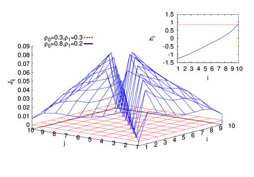
Figure 1: (Color online) Optimized $J_{ij}$ for the SSEP model with open boundaries for $\rho_{0}=\rho_{1}$ (dotted red line) and for $\rho_{0}\neq\rho_{1}$ (solid blue line). The inset shows similar results for the optimized $h_{i}$

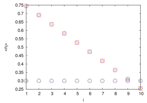
Figure 2: (Color online) Analytical and simulation results for the steady state density profile $\langle n_{i}\rangle$. Red squares $\square$ and orange crosses $\times$ correspond to the Monte Carlo procedure for densities $\rho_{0}=0.8$, $\rho_{1}=0.2$ using the optimized trial $\rho_{opt}(\mathbf{n})$ and the local equilibrium measure $\rho_{LE}(\mathbf{n})$ respectively, whereas blue diamonds $\Diamond$ are the analytical results, see Eq. (43). Purple triangles $\bigtriangleup$ correspond to the Monte Carlo procedure for densities $\rho_{0}=\rho_{1}=0.3$ using the equilibrium measure $\rho_{eq}(\mathbf{n})$, whereas black circles $\bigcirc$ are the analytical results.

We also measured the two-point correlation function $\langle n_{i}n_{j}\rangle_{c}\equiv\langle n_{i}n_{j}\rangle-\langle n_{i}\rangle\langle n_{j}\rangle$, obtaining the results shown in Fig. 3. Using again the exact measure $\rho_{ss}(\mathbf{n})$,one finds that the analytical prediction in the steady state for $1\leq i<j\leq L$ is derrida_leb

$$\langle n_{i}n_{j}\rangle_{c}=\displaystyle\frac{-(\rho_{0}-\rho_{1})^{2}(\frac{1}{\alpha+\gamma}+i-1)(\frac{1}{\beta+\delta}+L-j)}{(\frac{1}{\alpha+\gamma}+\frac{1}{\beta+\delta}+L-1)^{2}(\frac{1}{\alpha+\gamma}+\frac{1}{\beta+\delta}+L-2)}.$$ (44)

For large $L$, introducing macroscopic coordinates $i=Lx$ and $j=Ly$, this becomes, for $x<y$, $\langle n_{Lx}n_{Ly}\rangle_{c}=-x(1-y)(\rho_{0}-\rho_{1})^{2}/L$. As stated in derrida_leb , one may think that these weak, but long-range, correlations play no role in the macroscopic limit. However, they are responsible for a leading contribution in the variance of a macroscopic quantity such as the number of particles.

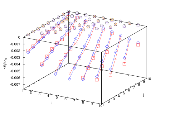
Figure 3: (Color online) Analytical and simulation results for the two-point correlation function $\langle n_{i}n_{j}\rangle_{c}$ in the steady state. Red squares $\square$ and orange crosses $\times$ correspond to the Monte Carlo procedure for densities $\rho_{0}=0.8$, $\rho_{1}=0.2$ using the optimized trial $\rho_{opt}(\mathbf{n})$ and the local equilibrium measure $\rho_{LE}(\mathbf{n})$ respectively, whereas blue diamonds $\Diamond$ are the analytical results, see Eq. (44). Purple triangles $\bigtriangleup$ correspond to the Monte Carlo procedure for densities $\rho_{0}=\rho_{1}=0.3$ using the equilibrium measure $\rho_{eq}(\mathbf{n})$, whereas black circles $\bigcirc$ are the analytical results.

As expected, Fig. 3 shows how the Monte Carlo procedure fits exactly with the analytical results for $\rho_{0}=\rho_{1}$ ($\langle n_{i}n_{j}\rangle_{c}=0$) because we are using the equilibrium measure in which no spatial correlations are present. In addition, for $\rho_{0}\neq\rho_{1}$ we see how the results obtained with the optimized measure are much closer to the exact analytical ones than those obtained with the local equilibrium assumption. This reflects the fact that with the optimized measure we are taking into account at least the two-site long-range correlations, which are not considered in the local equilibrium case. This shows that the physically motivated optimized trial is very good, at least regarding one- and two-point static spatial correlation functions. In this sense the out of equilibrium state of the SSEP can be thus fairly approximated by simple and intuitive quantities such as the local effective fields and two-site long-range interactions. Although more difficult to guess, one might of course add other terms to the trial function to improve the present agreement, for instance, higher order interaction terms, but the difficulty of the numerical minimization problem increases very rapidly.

V Conclusion

We have derived an exact relation for Markovian systems that generalizes the Hatano-Sasa relation but does not rely on the a priori knowledge of the stationary probability distribution, but rather on arbitrary trial functions for the stationary distribution. More generally, we have derived the detailed version of the fluctuation relation by identifying a generalized form of dual (adjoint) dynamics, generating the backward process that yields a trajectory-dependent entropy production. For systems described by Langevin dynamics, we have showed that the dual dynamics is also governed by a simple Langevin dynamics, which may be expressed directly in terms of the trial functions. One may also obtain in this context a version of the three extended detailed fluctuation theorems of Ref. Esposito .

Our approach leads to an infinite family of inequalities that generalize the second law, and suggests a variational principle for optimizing trial measures, in a quantitative and controlled way, to approximate nonequilibrium probability distributions. The optimization procedure we propose might be implemented numerically or even experimentally in order to infer nonequilibrium steady-state distributions in terms of intuitive physical quantities. To illustrate this, we have implemented this approximating scheme for the simple symmetric exclusion process in one dimension.

A particularly interesting case for applying this variational approach is to active matter unpublished , where it has been proposed recently to represent the complex energy exchanges in the system by a bath with equilibrium-like properties (Refs. jor ; leticia ; wolynes ). Another interesting and somewhat related system is that of current-driven vortices in superconductors with pinning. In this case the complex interplay of driving, quenched disorder and vortex-vortex interactions yields a variety of nonequilibrium dynamical regimes and transitions that may sometimes be successfully described by effective temperatures vortices . At any rate, the important property of these approximations is that there is a second law-type inequality associated with them.

Appendix A Three extended detailed fluctuation theorems

Using the dual dynamics of of Eq. (27), it is straightforward to derive an extension for the three fluctuation theorems of Ref. Esposito based, in our case, on smooth trial functions ${\rho_{\tt ref}}$ rather than the true steady-state measure ${\rho_{\tt ss}}$.

We define three trajectory dependent “entropy productions” using time-reversal ($R$) and the dual (adjoint) dynamics:

$$\mathcal{S}[\mathcal{T},\alpha] \equiv \ln{\mathcal{P}[\mathcal{T},\alpha]}-\ln\mathcal{P}^{R}[\mathcal{T},\alpha],$$ (45)

$${\mathcal{Y}}[\mathcal{T},\alpha] \equiv \ln{\mathcal{P}[\mathcal{T},\alpha]}-\ln{\left[\mathcal{P}^{{adj}}[\mathcal{T},\alpha]\right]^{R}},$$ (46)

$${\mathcal{W}}[\mathcal{T},\alpha] \equiv \ln{\mathcal{P}[\mathcal{T},\alpha]}-\ln{\mathcal{P}^{adj}[\mathcal{T},\alpha]},$$ (47)

so that by construction they satisfy the detailed fluctuation theorems,

$$\langle\mathcal{O}[\mathcal{T}]e^{-\mathcal{S}[\mathcal{T},\alpha]}\rangle={\langle\mathcal{O}[\mathcal{T}]\rangle}^{R},$$ (48)

$$\langle\mathcal{O}[\mathcal{T}]e^{-{\mathcal{Y}}[\mathcal{T},\alpha]}\rangle=\left[{\langle\mathcal{O}[\mathcal{T}]\rangle}^{{adj}}\right]^{R},$$ (49)

$$\langle\mathcal{O}[\mathcal{T}]e^{-{\mathcal{W}}[\mathcal{T},\alpha]}\rangle={\langle\mathcal{O}[\mathcal{T}]\rangle}^{{adj}},$$ (50)

where again $\mathcal{O}$ is an arbitrary functional of the trajectory.

For a system satisfying a Fokker-Planck process (23), it is easy to show using Eqs. (25), (III.3), and (15) that

$$\partial_{\tau}\mathcal{S} = \beta{\bf f}({\bf x};\alpha)\cdot\dot{{\bf x}}|_{t=\tau},$$ (51)

$$\partial_{\tau}{\mathcal{Y}} = \left[\dot{\alpha}\partial_{\alpha}{\phi_{\tt ref}}({\bf x},\alpha)+\varphi({\bf x};\alpha)\right]|_{t=\tau},$$ (52)

$$\partial_{\tau}{\mathcal{W}} = \left[\beta{\bf f}({\bf x};\alpha)\cdot\dot{{\bf x}}-\dot{\alpha}\partial_{\alpha}{\phi_{\tt ref}}({\bf x},\alpha)+\varphi({\bf x};\alpha)\right]|_{t=\tau},$$

with $\beta\equiv 1/T$. Therefore the total trajectory-dependent entropy production Ku may be written as

$$\partial_{\tau}\mathcal{S}=\partial_{\tau}{\mathcal{Y}}+\partial_{\tau}{\mathcal{W}}-2\varphi.$$ (54)

The corresponding integral fluctuation theorems for $\mathcal{S}$, ${\mathcal{Y}}$, and ${\mathcal{W}}$, particular cases of Eqs. (48), (49), and (50), respectively, read

$$\langle e^{-\mathcal{S}}\rangle=\langle e^{-{\mathcal{Y}}}\rangle=\langle e^{-{\mathcal{W}}}\rangle=1.$$ (55)

The first fluctuation theorem in Eq.(55) is the well-known integral fluctuation theorem for the total entropy production or Jarzynski relation, here generalized to arbitrary initial conditions and dynamics without detailed balance. The second one is the Hatano-Sasa extension discussed in detail in Sec. III, and the third one can be considered as an extension of the Speck and Seifert integral fluctuation theorem SpSe . We note, however, that the interpretation of ${\mathcal{Y}}$ and ${\mathcal{W}}$ as the nonadiabatic $\mathcal{S}_{na}$ and adiabatic $\mathcal{S}_{a}$ entropy production contributions, respectively, is lost due to the presence of $\varphi$, which does not vanish in the adiabatic limit if ${\rho_{\tt ref}}\neq{\rho_{\tt ss}}$.

When ${\rho_{\tt ref}}={\rho_{\tt ss}}$, ${\phi_{\tt ref}}=\phi$, and $\varphi=0$, and the three extended fluctuation theorems reduce to the three fluctuation relations described in Ref. Esposito . In this case, the dual dynamics becomes exactly the standard dual or adjoint ($\dagger$) dynamics, and up to boundary terms we can identify ${\mathcal{Y}}=\mathcal{S}_{na}$, ${\mathcal{W}}=\mathcal{S}_{a}$. In addition, we note that Eq. (27) reduces to the standard dual dynamics in its Langevin form by the simple replacement ${\phi_{\tt ref}}\to\phi$. The dual dynamics given here is therefore the natural and probably simplest generalization of the standard dual dynamics that does not rely on the knowledge of ${\rho_{\tt ss}}$.

References

- (1) S. F. Edwards, in: Granular Matter: An Interdisciplinary Approach, A. Mehta, Ed. (Springer-Verlag, New York 1994), p.121, and references therein.
- (2) J. Kurchan, J. Phys.: Condens. Matter 12, 6611 (2000).
- (3) D. Loi, S. Mossa and LF Cugliandolo, Soft Matter, Advance Article (2011) (in press).
- (4) S. Wang and P. G. Wolynes, Proc. Natl. Acad. Sci. USA 108, 15184 (2011).
- (5) A broad review with an emphasis in experimental results and applications is: F. Ritort, Séminaire Poincare 2, 193 (2004), a more technical one specialized in the Fluctuation Relation is: D. Evans and D. Searles, Adv. Phys. 51, 1529 (2002); See also G. Gallavotti, Statistical Mechanics A Short Treatise Series Texts and Monographs in Physics, Springer Verlag (1999).
- (6) D. J. Evans, E. G. D. Cohen, and G. P. Morriss, Phys. Rev. Lett. 71, 2401 (1993); D. J. Evans and D. J. Searles, Phys. Rev. E 50, 1645 (1994).
- (7) G. Gallavotti and E.G.D. Cohen, Phys. Rev. Lett. 74, 2694-2697 (1995); J. Stat. Phys. 80, 931-970 (1995).
- (8) J. Kurchan, J. Phys. A (Math. Gen.) 31, 3719 (1998);
- (9) P. I. Hurtado, C. Pérez-Espigares, J. J. del Pozo and P. L. Garrido, Proc. Natl. Acad. Sci. USA 108, 7704 (2011)
- (10) C. Jarzynski, Phys. Rev. Lett. 78, 2690 (1997); Phys. Rev. E 56, 5018 (1997).
- (11) G. E. Crooks, J. Stat. Phys. 90, 1481 (1998); G. E. Crooks, Phys. Rev. E 61, 2361 (2000).
- (12) T. Hatano, S. I. Sasa, Phys. Rev. Lett. 86, 3463 (2001); see also Oono ; foot1 .
- (13) Y. Oono, and M. Paniconi, Prog. Theor. Phys. Suppl. 130, 29 (1998), see S. Sasa and H. Tasaki, J. of Stat. Phys. 125, 125 (2006).
- (14) The Hatano-Sasa, together with Seifert Seifert and Speck-Seifert relations SpSe were very recently unified in three detailed fluctuation theorems through particular two-fold decompositions of the total entropy production, either using single Esposito or joint Reinaldo probability distributions for the entropy production contributions.
- (15) Hoover W.G.,Molecular Dynamics, Lecture Notes in Physics 258, edited by H. Araki et al. (Springer-Verlag, Heidelberg, 1986).
- (16) J. L. Lebowitz and P. G. Bergmann, Annals of Physics 1, 1 (1957).
- (17) R. Kawai, J. M. R. Parrondo, and C. Van den Broeck, Phys. Rev. Lett. 98, 080602 (2007); J. M. R. Parrondo, C. Van den Broeck and R Kawai, New J. Phys. 11, 073008 (2009).
- (18) U. Seifert, Phys. Rev. Lett. 95, 040602 (2005).
- (19) T. Speck and U. Seifert, J. Phys, A 38, L581 (2005).
- (20) M. Esposito and C. Van den Broeck, Phys. Rev. E 82 011143 (2010); C. Van den Broeck and M. Esposito, Phys. Rev. E 82, 011144 (2010); M. Esposito and C. Van den Broeck, Phys. Rev. Lett. 104, 090601 (2010).
- (21) N. Merhav and Y. Kafri, J. Stat. Mech. P12022 (2010).
- (22) G. Verley, R. Chetrite and D. Lacoste, J. Stat. Mech. P10025 (2011).
- (23) R. García-García, D. Domínguez, V. Lecomte, and A. B. Kolton, Phys. Rev. E 82, 030104 (2010); arXiv:1111.5369v2.
- (24) H. Risken; The Fokker-Planck equation, Springer-Verlag, 1984.
- (25) See, for example: R. Monasson and S. Cocco, Journal Computational Neuroscience 31 199 (2011); S. Cocco, R. Monasson and V. Sessak, Phys. Rev. E 83 051123 (2011)
- (26) B. Derrida, J.L. Lebowitz and E. R. Speer, J. Stat. Phys. 107 599-634 (2002)
- (27) B. Derrida, M. R. Evans, V. Hakim and V. Pasquier, J. Phys. A 26 1493 (1993)
- (28) J. Nocedal, Mathematics of Computation 35 773-782 (1980)
- (29) C. Pérez-Espigares, A. B. Kolton and J. Kurchan (in preparation).
- (30) A. B. Kolton, R. Exartier, L. F. Cugliandolo, D. Dominguez and N. Gronbech-Jensen, Phys. Rev. Lett. 89, 227001 (2002).
- (31) V. Y. Chernyak, M. Chertkov and C. Jarzynski, J. Stat. Mech. P08001 (2006).
- (32) This seems to be related to the expression, valid for systems that satisfy detailed balance, obtained in: T. Sagawa and M. Ueda, Phys Rev Lett 104, 090602 (2010). Here the difference is that we are trying to approximate driven systems whose stationary measure we do not know.
- (33) L. Bertini, A. De Sole, D. Gabrielli, G. Jona-Lasinio, and C. Landim, Phys. Rev. Lett. 87, 040601 (2001); J. Stat. Phys 107, 635 (2002).