Wireless Connectivity and Capacity

Abstract.

Given $n$ wireless transceivers located in a plane, a fundamental problem in wireless communications is to construct a strongly connected digraph on them such that the constituent links can be scheduled in fewest possible time slots, assuming the SINR model of interference.

In this paper, we provide an algorithm that connects an arbitrary point set in $O(\log n)$ slots, improving on the previous best bound of $O(\log^{2}n)$ due to Moscibroda. This is complemented with a super-constant lower bound on our approach to connectivity. An important feature is that the algorithms allow for bi-directional (half-duplex) communication.

One implication of this result is an improved bound of $\Omega(1/\log n)$ on the worst-case capacity of wireless networks, matching the best bound known for the extensively studied average-case.

We explore the utility of oblivious power assignments, and show that essentially all such assignments result in a worst case bound of $\Omega(n)$ slots for connectivity. This rules out a recent claim of a $O(\log n)$ bound using oblivious power. On the other hand, using our result we show that $O(\min(\log\Delta,\log n\cdot(\log n+\log\log\Delta)))$ slots suffice, where $\Delta$ is the ratio between the largest and the smallest links in a minimum spanning tree of the points.

Our results extend to the related problem of minimum latency aggregation scheduling, where we show that aggregation scheduling with $O(\log n)$ latency is possible, improving upon the previous best known latency of $O(\log^{3}n)$. We also initiate the study of network design problems in the SINR model beyond strong connectivity, obtaining similar bounds for biconnected and $k$-edge connected structures.

1. Introduction

A key architectural goal in wireless adhoc networks is to ensure that each node in the network can communicate with every other node (perhaps by routing through other nodes). This requires that the nodes be connected through a communication overlay. The problem can be abstracted as such: Given $n$ points on the plane (each representing a wireless node), how efficiently can one ensure connectivity among the points?

The notion of efficiency in a wireless setting is crucially dependent on that distinguishing feature of wireless networks: interference. Two or more simultaneous communications in the same wireless channel interfere with each other, potentially destroying all or some of the communications. Thus, easy as it might be to come up with a set of links (a link is an directed edge between two nodes) that connect the $n$ nodes, it is highly unclear whether or not one can schedule these links in a small amount of time. This fundamental problem has been the focus of substantial amount of research [19, 21, 18, 3, 1].

The model of interference is of course a crucial aspect. Traditionally, all theoretical results have been in graph-based models, with either fixed radii (unit-disc graphs and quasi-unit disc graphs) and variable radii (geometric radio networks and protocol model), while engineering research has focused on largely non-algorithmic studies in more complex models. We adopt the SINR (signal to noise and interference ratio) model, a.k.a. the physical model, of interference. The main differences are two-fold: the received signal is a decaying function of distance (rather than being on/off), and interferences from multiple transmitters sum up. While more involved analytically, the SINR models is known to be more realistic than graph-based ones, as shown theoretically as well as experimentally [6, 17, 20].

The first worst-case guarantee for wireless connectivity in the SINR model was provided by Moscibroda and Wattenhofer [19], who showed how to construct a strongly connected set of links that can be scheduled in $O(\log^{4}n)$ slots. This was improved to $O(\log^{3}n)$ in [21] and finally to $O(\log^{2}n)$ by Moscibroda [18], which is the best bound currently known.

Our main result is the following: Any minimum spanning tree (arbitrarily oriented) on $n$ nodes on the plane can be scheduled in $O(\log n)$ slots. This immediately leads to a $O(\log n)$ worst-case bound for strong connectivity, by orienting the tree towards an arbitrary root and then using the same tree with the orientation reversed. Thus we improve the connectivity bound by a $\log n$ factor, while giving at the same time a simple characterization of the resultant network in terms of the natural MST structure.

The connectivity problem is closely related to the capacity of a wireless network, a subject of a vast literature. The computational throughput capacity of a network is the sustained rate at which data can be aggregated to an information sink, which is really the raison d’être of wireless sensor networks. At each time step, data is introduced at each source node. If the aggregation function is compressible, like sum or max, only one item of data needs to be forwarded on each link. A short schedule that is repeated as needed yields high throughput using buffering. Bounds for the connectivity problem lead therefore immediately to equivalent bounds for worst-case capacity of wireless network (for compressible functions) [18].

Indeed, this particular application also highlights the specific benefits of adopting the SINR model. The best known bound on the average-case capacity in the SINR model is $\Omega(1/\log n)$, given in the influential work of Gupta and Kumar [7]. On the other hand, whereas the average case throughput capacity in the protocol model is $\Theta(1/\log n)$ [7], the worst-case capacity is only $\Theta(1/n)$ [18].

We also study a variation of the connectivity problem inspired by the sensor networking application mentioned above is known as minimum-latency aggregation scheduling. In this variation, one seeks a tree aggregating to a information sink (as before), but with the additional requirement that links must be scheduled after all links below them in the tree are scheduled. A straightforward modification of our algorithm achieves this in optimal $O(\log n)$ slots, improving on the $O(\log^{3}n)$ result previously known [16].

We conjecture that a logarithmic bound is necessary for connectivity. One reason is that it matches the average-case bound, which has been a highly researched topic [7]. We also give a construction that shows that our approach cannot yield a constant upper bound. It is distinguished from all previous lower bound constructions in the SINR model in that it is (necessarily) not based on showing that pairs of links are incompatible. Without being able to show the existence of large “cliques”, hardness results in the SINR with power control are hard to come by.

An important – and perhaps surprising – feature of our method is that it allows for bidirectional communication. Namely, the links scheduled in each slot can communicate in either direction without affecting or being affected by the other scheduled links. This is important in a communication setting because of the need to supply acknowledgements and flow control, and is sometimes viewed as indispensable. The previously studied algorithms [19, 21, 18] all assumed unidirectional communication. In fact, it was taken for granted that unidirectionality could not be avoided, sometimes with references to lower bounds from graph-based models [21]. Our algorithm uses different power for the two directions of each link; we show that to be unavoidable by constructing instances for which the use of symmetric power on bidirectional links forces the use of $\Omega(n)$ slots.

Power assignments are yet another important issue in wireless protocols. It is preferable if power settings are locally computable. A power assignment is oblivious if it depends only on the length of the respective link. Recently, a $O(\log n)$-slot connectivity algorithm was claimed that used a particular oblivious power assignment [15]. Unfortunately, there are problems with the proof (specifically, in Lemma 5 whose proof is not in the conference version) as acknowledged by one of the authors [14]. Actually, that general approach is bound to fail; namely, we show that essentially all oblivious power assignments (including the one used in [15]) require $\Omega(n)$ slots in the worst case.

On the other hand, when the edge lengths in the MST differ by a factor of at most $\Delta$, then combining the results here with recent work [9] gives a $O(\log n(\log\log\Delta+\log n))$ slot connectivity algorithm that uses a certain oblivious power assignment called mean power.

We use our approach as a starting point for the first excursion into network design problems beyond strong connectivity. By applying the connectivity routine a constant number of times, we find that we can solve other connectivity problems with asymptotically the same number of slots, including biconnectivity and $k$-edge connectivity.

Outline of the paper.

We introduce the SINR model and related notation in Sec. 2, followed by quick overview of related work in Sec. 3. The connectivity algorithm is given in Sec. 4, with a subsection on a limitation result. We extend the method to a bi-directional model of communication in Sec. 5, and examine the power of oblivious power in Sec. 6. Extensions to other connectivity problems are treated in Sec. 7.

2. Model and Preliminaries.

Given is a set $P=\{p_{1},p_{2},\ldots,p_{n}\}$ of points on the Euclidean plane. A link $\ell=(s,r)$ is a directed edge from point $s$ (the “sender”) to point $r$ (the “receiver”). The goal is compute a set of links that strongly connect $P$ and to schedule them in $O(\log n)$ slots.

The distance between two points $x$ and $y$ is denoted $d(x,y)$. The asymmetric distance from link $\ell=(s,r)$ to link $\ell^{\prime}=(s^{\prime},r^{\prime})$ is the distance from $\ell$’s sender to $\ell^{\prime}$’s receiver, denoted $d_{\ell\ell^{\prime}}=d(s,r^{\prime})$. The length of link $\ell$ is denoted simply $\ell$. For a link set $L$, let $\Delta$ denote the ratio between the maximum and minimum length of a link in $L$.

When a point $s$ transmits as a sender of link $\ell$, it uses some transmission power $P_{\ell}$. We adopt the physical model (or SINR model) of interference: a communication over a link $\ell=(s,r)$ succeeds if and only if the following condition holds:

(1) $$\frac{P_{\ell}/\ell^{\alpha}}{\sum_{\ell^{\prime}\in S\setminus\{\ell\}}P_{\ell^{\prime}}/d_{\ell^{\prime}\ell}^{\alpha}+N}\geq\beta,$$

where $\alpha>2$ is the path loss constant, $N$ is a universal constant denoting the ambient noise, $\beta\geq 1$ denotes the minimum SINR (signal-to-interference-noise-ratio) required for a message to be successfully received, and $S$ is the set of concurrently scheduled links in the same slot with $\ell$. We say that $S$ is SINR-feasible (or simply feasible) if (1) is satisfied for each link in $S$.

We will use the notion of affectance of [10], as refined in [13], which is a scaled interference measure from one link on another, defined as

$$a_{\ell}(\ell^{\prime})=\min\left\{1,c_{\ell^{\prime}}\frac{P_{\ell}/d_{\ell\ell^{\prime}}^{\alpha}}{P_{\ell^{\prime}}/\ell^{\prime\alpha}}\right\}$$

where $c_{\ell^{\prime}}=\beta/(1-\beta N{\ell^{\prime}}^{\alpha}/P_{\ell^{\prime}})$ is a constant depending only on the length and power of the link $\ell^{\prime}$. As in previous work [19, 21, 18, 12], we assume that powers can be scaled up as needed, which implies that the effect of the noise $N$ (and the coefficient $c_{\ell^{\prime}}$) can be ignored. It holds that $\ell^{\prime}$ is feasible in $S$ iff

(2) $$\sum_{\ell\in S}a_{\ell}(\ell^{\prime})\leq 1,$$

where $S$ is the set of simultaneously transmitting links. We will sometimes use this version of the SINR constraint instead of Eqn. 1.

For a set of points $P$, we will use $T(P)$ to denote a minimum spanning tree over the points in $P$. We will simply use $T$ when $P$ is clear from the context. Naturally, $T$ contains undirected edges, but when scheduling directed links, we need to orient $T$ in some way. When no ambiguity arises, we will simply use $T$ to describe a particular oriented version of $T$.

3. Related Work

Abstract problems capturing aspects of wireless networks have a long history, but the adoption of the SINR model in theoretical analysis has been a comparatively recent phenomenon. The first rigorous worst case results were achieved in the seminal work of Moscibroda and Wattenhofer [19] (which involved the problem studied in this paper). Ever since, numerous paper have appeared on the SINR model. For a recent overview, see [5]. Apart from the connectivity, another fundamental problem is the capacity problem, where one wants to find the maximum feasible subset of a given set of links. First rigorous results for the capacity problem were established in [4], followed by a number of other results. Kesselheim achieved a breakthrough recently by proving the first $O(1)$-approximation algorithm for capacity with power control [12], whose techniques we adopt into our analysis. In this regard, this work can be considered to bring the approaches to connectivity and capacity together. Other recent progresses made include a $O(1)$-approximation capacity algorithm for oblivious powers [9], and the study of topological properties of wireless communication maps [11].

4. $O(\log n)$ connectivity in the SINR model

The starting point of our analysis is a criteria for wireless capacity recently developed by Kesselheim [12]. Kesselheim showed that any set of links for which this criteria holds (defined in Eqn. 4 below) can be scheduled in a single slot, and provided an efficient algorithm to do so. We shall call this algorithm Schedule, which is described in Section 3 of [12]. For reference, we also include the algorithm in Appendix A.

Our approach is as follows. We show, via a related criteria, that given any $T^{\prime}\subseteq T(P)$, Eqn. 4 holds for a constant fraction of the links in $T^{\prime}$. Thus, a constant fraction of the tree can be scheduled in a single step (and this holds recursively). Naturally this process will end in $O(\log n)$ steps. Our analysis applies to any orientation of $T$. Thus to achieve a strongly connected network, we simple schedule two trees. One is a copy of $T$ oriented towards some arbitrary root, another one oriented away from the same root. Thus any two nodes in the network can communicate by first routing from the source to the root, and then routing from the root to the destination.

Our goal is then to prove the following.

Theorem 1.

Let $P$ be any set of points on the Euclidean plane. Let $T=T(P)$ be a minimum spanning tree on the points of $P$, arbitrarily oriented. Then algorithm Connect schedules $T$ in $O(\log n)$ slots.

Algorithm 1 Connect(An arbitrarily oriented MST $T$ on point set $P$)

1:  $L\leftarrow T$

2:  while $L\neq\emptyset$ do

3:     Use Algorithm Schedule to find a feasible subset $L^{\prime}\subseteq L$

4:     $L\leftarrow L\setminus L^{\prime}$

5:  end while

For two links $\ell,\ell^{\prime}$, define $d(\ell,\ell^{\prime})=\min\{d_{\ell\ell^{\prime}},d_{\ell^{\prime}\ell}\}$. For links $\ell\leq\ell^{\prime},\ell\neq\ell^{\prime}$ define the function $f_{\ell}(\ell^{\prime})=\min\left\{1,\frac{\ell^{\alpha}}{d(\ell,\ell^{\prime})^{\alpha}}\right\}$. Let $f_{\ell}(\ell)=0$ and for $\ell>\ell^{\prime}$ let $f_{\ell}(\ell^{\prime})=0$. The function $f_{\ell}(\ell^{\prime})$ can be thought of as a measure of how badly the link $\ell$ might affect link $\ell^{\prime}$ if they were to transmit simultaneously.

We call a set of links $L$ amenable if the following holds: for any link $\ell=(s,r)$ ($\ell$ not necessarily a member of $L$),

(3) $$\sum_{\ell^{\prime}\in L,\ell^{\prime}\geq\ell}f_{\ell}(\ell^{\prime})\leq\rho$$

for some constant $\rho$ to be chosen later. The concept of an amenable set is closely related to the following theorem due to Kesselheim (the connection is made explicit in Lemma 3).

Theorem 2 ([12]).

Assume $L^{\prime}$ is a set of links such that for all $\ell^{\prime}\in L^{\prime}$,

(4) $$\sum_{\ell\in L^{\prime},\ell\leq\ell^{\prime}}f_{\ell}(\ell^{\prime})\leq\gamma$$

for a constant $\gamma=\frac{1}{4\cdot 3^{\alpha}\cdot(4\beta+2)}$. Then, $L^{\prime}$ is feasible and there exists a polynomial time algorithm to find a power assignment to schedule $L^{\prime}$ in a single slot.

Moreover, for any given set $L$ assume $S$ is the largest feasible subset of $L$. Then Schedule finds a $L^{\prime\prime}$ of size $\Omega(S)$ for which Eqn. 4 holds.

Lemma 3.

If a set $L$ of size $n$ is amenable, then there are $\Omega(n)$ links in $L$ that can be scheduled in a single slot.

Proof.

Since $L$ is amenable, then by definition $\sum_{\ell\in L}\sum_{\ell^{\prime}\geq\ell}f_{\ell}(\ell^{\prime})\leq n\rho$. Rearranging, we get $\sum_{\ell^{\prime}\in L}\sum_{\ell\leq\ell^{\prime}}f_{\ell}(\ell^{\prime})\leq n\rho$. By an averaging argument, there must be a set $S$ of at least $n/2$ links for which

(5) $$\sum_{\ell\leq\ell^{\prime}}f_{\ell}(\ell^{\prime})\leq 2\rho\ .$$

This is almost exactly Eqn. 4 except for the use of a different constant. To achieve the correct constant, a simple sparsification suffices. Start an empty set. Go through links in $S$ in increasing order of length, putting the link in the first set in which Eqn. 4 holds. Start a new set if necessary. Clearly, no more that $\frac{2\rho}{\gamma}$ sets will be necessary.

Thus, a set of size $\frac{n\cdot\gamma}{4\rho}$ can be found for which Eqn. 4 holds. ∎

The most important step is to prove that $T$ is amenable.

Lemma 4.

Let $T^{\prime\prime}\subseteq T$ where $T=T(P)$ is a minimum spanning tree on the points in $P$. Then $T^{\prime\prime}$ is amenable.

Proof.

Consider any link $\ell$ (not necessarily in $T$) and assume without of loss of generality that its length is $1$. We can do this because scaling all links to make $\ell$ of length $1$ does not change the values of the function $f_{\ell}(\ell^{\prime})$. To prove amenability, we thus have to only consider links in $T^{\prime\prime}$ of length at least $1$. Let $T^{\prime}$ be this set and let $P^{\prime}$ be the points that are incident to at least one edge in $T^{\prime}$.

First we claim,

Lemma 5.

Any disc of radius $c_{1}=1/4$ contains at most 9 points from $P^{\prime}$.

Proof.

Let $D$ be a disc of radius $c_{1}$ and let $P_{D}$ be the set of points from $P^{\prime}$ in $D$.

We first observe that no two points $p_{1},p_{2}\in P_{D}$ have a common neighbor in $T^{\prime}$. If $p_{1}$ and $p_{2}$ were neighbors in $T$ then a common neighbor would imply a cycle, while if they were non-neighbors, replacing either of the edges to the common neighbor by the edge $(p_{1},p_{2})$ results in a cheaper spanning tree (since $d(p_{1},p_{2})\leq 2c_{1}<1$). Since each point in $P_{D}$ has a neighbor in $T^{\prime}$, it holds that $|N(P_{D})|\geq|P_{D}|$ (where $N(X)=N_{T^{\prime}}(X)=\{p\in P^{\prime}:\exists x\in X,(x,p)\in T^{\prime}\}$ denotes the neighborhood of a point set $X$ in $T^{\prime}$).

Let $c$ be the center of $D$, and consider any pair of points $a,b\in N(P_{D})$. We aim to show that the angle $\angle acb>\pi/5$, which implies the lemma. Let $p_{a}$ ($p_{b}$) be the unique neighbor of $a$ ($b$) in $T$. We observe first that the unique path in $T$ between $p_{a}$ and $p_{b}$ goes through neither $a$ nor $b$, since if it did, say through $a$, then replacing $(p_{a},a)$ by $(p_{a},p_{b})$ results in a smaller tree.

Consider now the triangle $\triangle abc$. Let $\alpha=\angle cab$, $\beta=\angle abc$, $\gamma=\angle bca$, and denote $|p_{1}p_{2}|=d(p_{1},p_{2})$, for points $p_{1}$ and $p_{2}$. Note that $|ab|\geq d(a,p_{a})\geq 1$, as we could otherwise delete the edge $ap_{a}$ and add $ab$ to get a better tree. Similarly, $|ab|\geq d(b,p_{b})\geq 1$. From the triangular inequality, our observations above, and the fact that $|ab|\geq 1$, we have that

$$|ac|\leq d(a,p_{a})+d(p_{a},c)\leq|ab|+c_{1}\leq|ab|(1+c_{1})\ ,$$

and similarly $|bc|\leq{|ab|}(1+c_{1})$. By the sine law, $\sin\alpha/\sin\gamma=|bc|/|ab|\leq 1+c_{1}$, and $\sin\beta/\sin\gamma=|ac|/|ab|\leq 1+c_{1}$. For $c_{1}=1/4$, this implies that since $2\pi=\alpha+\beta+\gamma\leq\gamma+2\arcsin(5/4\cdot\sin\gamma)$, computation shows that $\gamma>\pi/5$ as claimed. ∎

Now for $\ell=(s,r)$, $\sum_{\ell^{\prime}=(s^{\prime},r^{\prime})\in T^{\prime},\ell^{\prime}\geq\ell}f_{\ell}(\ell^{\prime})\leq\sum_{p\in P^{\prime}}\left(\min\left\{1,\frac{1}{d(p,s)^{\alpha}}\right\}+\min\left\{1,\frac{1}{d(p,r)^{\alpha}}\right\}\right).$ Thus it suffices to upper bound $\sum_{p\in P^{\prime}}\min\left\{1,\frac{1}{d(p,x)^{\alpha}}\right\}$ for any arbitrary point $x$ by a constant to get the required bound.

Now take concentric circles $C_{0},C_{1}\ldots$ around $x$ such that the $t^{th}$ circle has radius $t+1$. The proof of the following fact can be found in Appendix B.

Lemma 6.

$C_{0}$ can be covered by $O(1)$ circles of radius $c_{1}$ (where $c_{1}$ is the constant from Lemma 5). The annulus $C_{t}\setminus C_{t-1}$ can be covered by $O(t)$ circles of radius $c_{1}$, for $t\geq 1$.

Thus by Lemma 5, there are at most $O(t)$ points from $P^{\prime}$ in $C_{t}\setminus C_{t-1}$. Similarly, $C_{0}$ can be covered by $O(1)$ circles of radius $c_{1}$ (see Lemma 6) and thus contains $O(1)$ points from $P^{\prime}$.

The distance to $x$ from any point in $C_{t}\setminus C_{t-1}$ is at least $t$. Then,

$$\sum_{p\in P^{\prime}}\min\left\{1,\frac{1}{d(p,x)^{\alpha}}\right\}$$

$$=|p\in P^{\prime}\cap C_{0}|\cdot 1+\sum_{t\geq 1}\sum_{p\in P^{\prime}\cap(C_{t}\setminus C_{t-1})}\frac{1}{d(p,x)^{\alpha}}$$

$$\leq O(1)+O\left(\sum_{t\geq 1}t\frac{1}{t^{\alpha}}\right)=O(1)\ ,$$

for $\alpha>2$. This completes the proof of Lemma 4, assuming that $\rho$ is at least twice the implicit constant in the bound above. ∎

Theorem 1 now follows easily. By Lemma 4, the remaining set of links at each step of the algorithm is amenable. Thus, by Lemma 3, a constant factor of these links are feasible, and by Theorem 2, a constant factor of those will be scheduled by Connect. Clearly, this process terminates in $O(\log n)$ steps.

Remark. We note that the assumption $\alpha>2$ is necessary. Indeed, suppose points are placed at all integer coordinates within a large circle, so all links will be of at least unit length. Then, when $\alpha\leq 2$, it can be shown with standard methods that there is no feasible subset of links of size larger than $\Omega(n/\log n)$.

4.1. A lower bound on our approach

It is easy to construct an example where a link in $T(P)$ violates Eqn. 4 (below, the set $G_{1}$ provides an example of that). However, this still leaves open the possibility that the spanning tree can be partitioned into a small number of subsets (for example, a constant number of subsets) such that Eqn. 4 holds for each of them, thus improving upon the $O(\log n)$ result. In the following theorem, we show that one cannot partition all the points into a constant number of subsets. This, naturally, is not a lower bound on the connectivity problem, just on our particular approach.

Theorem 7.

For any number $c$, there exists a set of points on the line such that the minimum spanning tree $T$ cannot be partitioned into $\leq c$ sets $S_{1},S_{2}\ldots S_{c}$ such that Eqn. 4 holds for each $S_{i}$.

Proof.

For $t\geq 1$, we will recursively construct gadgets $G_{t}$ such that a spanning tree on $G_{t}$ cannot be partitioned into $t$ sets for which Eqn. 4 holds.

Since we are considering points on a line, the minimum spanning tree is simply the edges connecting each point to its immediate neighbors to the right and left. Our theorem holds for any orientation of the links.

A gadget $G$ is simply a set of points located on a line, with an implicit ordering from the left to the right. We will often use $G$ to mean a translated copy of $G$ as well, which will be clear from the context. For two gadgets $F$ and $G$, we will use $F\oplus G$ to denote the joining of the two gadgets, which is a new gadget with $|F|+|G|-1$ points. The first (starting from the left) $|F|$ points are a copy of $F$, and the last $|G|$ points are a translated copy of $G$. In other words, the $|F|^{th}$ point is both the ending point of the gadget $F$ and the starting point for the copy of gadget $G$. For any collection of points (or gadget) $G$, let $L(G)$ be the diameter of $G$.

For a gadget $G$, we use $G(b)$ to mean a copy of the gadget scaled by a factor of $b$. For example, if $G=\{-10,0,1,2.5\}$, then $G(10)=\{-100,0,10,25\}$.

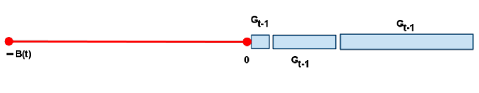
Figure 1. Construction of $G_{t}$ from copies of $G_{t-1}$. We join a number of copies of $G_{t-1}$, each succeeding copy scaled must larger than all the copies before it combined. All this is preceded by a huge new link between points $-B(t)$ and $0$ ($B(t)$ is very large)

We are ready to describe our construction. $G_{1}$ contains the points $\{-28,0,2,6,14\}$. For a gadget $G$, define $\rho(G)=\min_{\ell\in T(G)}\frac{\ell^{\alpha}}{{\hat{d}_{\ell}(G)}^{\alpha}}$ where $\hat{d}_{\ell}(G)$ is the maximum distance from either end point of $\ell$ to the left most point in $G$. It is easy to verify that $\rho(G)\leq 1$. Now $G_{t}$ is constructed by joining copies of $G_{t-1}$ (each copy scaled much larger than preceding copies) and preceding all of it with a new point, such that the distance between the new point and the beginning of the copies of $G_{t-1}$ is humongous. This is informally depicted in Fig. 1.

To formally define $G_{t}$, we first define $G^{\prime}_{t}=\oplus_{1\leq i\leq I(t)}G_{t-1}(h(i))$. The value of $I(t)$ is set to $\lceil\frac{8^{\alpha}\gamma}{\cdot\rho(G_{t-1})}\rceil$ where $\gamma$ is the constant from Eqn. 4. The scaling factors are defined as such: $h(1)=1$, $h(j)$ (for $j>1$) is chosen such that $\min_{\ell\in T(G_{t-1}(h(j)))}\ell=2L(\oplus_{1\leq i\leq j-1}G_{t-1}(h(i)))$. Let $G^{\prime}_{0}$ be $G^{\prime}_{t}$ translated so that its left most point is at location $0$. Define the number $B(t)=4L(G^{\prime}_{t})$. Then $G_{t}=\{-B(t)\}\cup G^{\prime}_{0}$, i.e., a single point at location $-B(t)$, followed by the gadget $G^{\prime}_{0}$.

Define the partition number $P(G)$ as the minimum number of partitions of a link set required so that Eqn. 4 holds for each set. We claim:

Claim 8.

$P(G_{1})\geq 2$ and $P(G_{t})\geq 1+P(G_{t-1})$ for all $t\geq 1$.

Combined, these two claims clearly prove the theorem. The claim about $G_{1}$ is easy to verify by direct computation. Let us prove the inductive step. For $G_{t}$ consider the left-most link $\ell_{g}$ in $T=T(G_{t})$. This is of course a link of length $B(t)$ which is by construction the unique largest link in $G_{t}$ (since $B(t)=4L(G^{\prime}_{t})$). Thus $\{\ell\in T:\ell<\ell_{g}\}=T\setminus\{\ell_{g}\}$. We claim that $\frac{\ell^{\alpha}}{d(s,r_{g})^{\alpha}}+\frac{\ell^{\alpha}}{d(s_{g},r)^{\alpha}}\geq\frac{\rho(G(t-1))}{2^{\alpha}}$ for all $\ell\in T\setminus\{\ell_{g}\}$. To see this, consider any $\ell\neq\ell_{g}\in T$. Now $\ell$ is of course part of the $j^{th}$ copy of $G_{t-1}$ for some $j\geq 1$. Now let $d^{\prime}=\min\{d(s,r_{g}),d(s_{g},r)\}$. We can observe that $d^{\prime}\leq\hat{d}_{\ell}(G_{t-1}(h(j))+L(\oplus_{1\leq i\leq j-1}G_{t-1}(h(i)))$. By construction, $\hat{d}_{\ell}(G_{t-1}(h(j))\geq\ell>L(\oplus_{1\leq i\leq j-1}G_{t-1}(h(i)))$ and thus $\frac{\ell^{\alpha}}{d(s,r_{g})^{\alpha}}+\frac{\ell^{\alpha}}{d(s_{g},r)^{\alpha}}\geq\frac{\ell^{\alpha}}{d^{\prime\alpha}}\geq\frac{\rho(G_{t-1})}{2^{\alpha}}$ (by definition of $\rho(G_{t-1}$)) proving the claim.

Given this and noticing the value of $I(t)$ chosen in the construction of $G^{\prime}_{t}$, it is clear that there must be some $1\leq j\leq I(t)$ such that no link in $T(G_{t-1}(h(j)))$ is in the same set as $\ell_{g}$. This completes the proof of the claim and the theorem. ∎

5. Bi-directionality

We have worked with the uni-directional model of wireless communication so far, where the links are directed from a sender to a receiver. The bi-directional model, in contrast, has two-way half-duplex communication between the nodes of a link in the same slot. The advantage of this model is that it simplifies one-hop communication protocols. Two-way communication in a single slot without worrying about mutual interference can be achieved in practice in more than one way, and we simply take that as given. The difficulty arises in that interferences from other links are now potentially much larger, since we have to take into account both directions of each link.

We can model the bi-directional case as follows: $L$ contains $n$ pairs $\ell=\{n_{1},n_{2}\}$. These two points implicitly define two unidirectional links $\ell_{1}=(n_{1},n_{2})$ and $\ell_{2}=(n_{2},n_{1})$. Each pair can be associated with two power levels $P_{\ell_{1}}$ and $P_{\ell_{1}}$, to be used by $\ell_{1}$ and $\ell_{2}$ respectively. We consider a set of pairs $L^{\prime}$ feasible if for all $\ell\in L^{\prime}$,

$$\frac{P_{\ell_{i}}/(\ell_{i})^{\alpha}}{\sum_{\ell^{\prime}\in L^{\prime}\setminus\{\ell\}}\sum_{k=1}^{2}P_{\ell^{\prime}_{k}}/(d_{\ell^{\prime}_{k}\ell_{i}})^{\alpha}+N}\geq\beta\quad\mathrm{for}i\in\{1,2\},$$

or equivalently,

$$\sum_{\ell^{\prime}\in L^{\prime},\ell^{\prime}\neq\ell}(a_{\ell^{\prime}_{1}}(\ell_{i})+a_{\ell^{\prime}_{2}}(\ell_{i}))\leq 1\quad\mathrm{for}i\in\{1,2\},$$

where affectances are as defined for the unidirectional case.

We differentiate two versions of the bi-directional model. In the symmetric model, we insist that $P_{\ell_{1}}=P_{\ell_{2}}$ for each $\ell$. With this restriction, the model is essentially equivalent to the one introduced in [2]. Without such a restriction, we call it the asymmetric model, which was briefly mentioned in [12].

First we show,

Theorem 9.

There is an instance that requires $\Omega(n)$ slots for connectivity in the symmetric bi-directional model.

Proof.

Consider the pointset $x_{0},\ldots,x_{n-1}$ given by $x_{0}=0,x_{1}=1$ and for $i\geq 2$, $x_{i}=2x_{i-1}^{2}$. Observe that $x_{m}-x_{m-1}>x_{m-1}^{2}$. Consider any two pairs $\ell=\{x_{i},x_{j}\}$ and $\ell^{\prime}=\{x_{k},x_{m}\}$, and assume without loss of generality that $m\geq\max(i,j,k)$. Thus, there must be indices $a,b,c,d\in\{1,2\}$ such that $d_{\ell_{a}\ell^{\prime}_{b}}\leq x_{m-1}$ and $d_{\ell^{\prime}_{c}\ell_{d}}\leq x_{m-1}$.

On the other hand $\ell^{\prime}_{b}\geq x_{m}-x_{m-1}$ and $\ell_{d}\geq 1$.

Then,

$$a_{\ell_{a}}(\ell^{\prime}_{b})\cdot a_{\ell^{\prime}_{c}}(\ell_{d})=\frac{P_{\ell_{a}}/d_{\ell_{a}\ell^{\prime}_{b}}^{\alpha}}{P_{\ell^{\prime}_{b}}/(\ell^{\prime}_{b})^{\alpha}}\cdot\frac{P_{\ell^{\prime}_{c}}/d_{\ell^{\prime}_{c}\ell_{d}}^{\alpha}}{P_{\ell_{d}}/(\ell_{d})^{\alpha}}$$

$$=\left(\frac{\ell_{d}\ell^{\prime}_{b}}{d_{\ell^{\prime}_{c}\ell_{d}}d_{\ell_{a}\ell^{\prime}_{b}}}\right)^{\alpha}\geq\left(\frac{x_{m}-x_{m-1}}{x^{2}_{m-1}}\right)^{\alpha}>1\ .$$

Thus, any pair of links must be scheduled in different slots. ∎

In surprising contrast to the above strong lower bound in the symmetric model,

Theorem 10.

In the asymmetric bi-directional model, any set of $n$ points can be strongly connected in $O(\log n)$ slots.

The argument in Section 4 is as follows. First, we show that $T^{\prime}\subseteq T$ is amenable. Then we find a large subset for which Eqn 4 holds, and finally, we schedule it in one slot. The main difference in the bi-directional case is that we have to choose pairs in a feasible set, i.e., for any pair $\ell$ that we want to connect, we have to include $\ell_{1}$ and $\ell_{2}$ in the same slot. Note that since, $\ell_{1}$ and $\ell_{2}$ have no effect on each other, we can define $f_{\ell_{i}}(\ell_{k})=0$ for $i,k\in\{1,2\}$. The new definition of amenability is thus,

(6) $$\sum_{\ell^{\prime}\in L,\ell^{\prime}\geq\ell}\sum_{j=1}^{2}\sum_{k=1}^{2}f_{\ell_{j}}(\ell^{\prime}_{k})\leq\rho$$

for a constant $\rho$.

We first need to verify that Lemma 4 still holds with the new definition. This happens to be easy. Indeed, the proof of Lemma 4 does not use the dichotomy between sender and receiver, and thus automatically holds (up to a factor of 4). It is easy to see that the argument in Lemma 3 continues to hold with minor differences.

Finally, we need to show that Thm. 2 still holds with the new definition, i.e., the algorithm Schedule can still successfully find and schedule the link set thus selected. The algorithm Schedule is robust in relation this, as [12] points out.

More specifically, to show that Schedule works for the bi-directional variant, we need the following version of Thm. 2:

Proposition 5.1.

Assume $L^{\prime}$ is a set of pairs such that for all $\ell^{\prime}\in L^{\prime}$,

(7) $$\sum_{\ell\in L^{\prime},\ell\leq\ell^{\prime}}\sum_{j=1}^{2}\sum_{k=1}^{2}f_{\ell_{j}}(\ell^{\prime}_{k})\leq\gamma$$

for a constant $\gamma=\frac{1}{4\cdot 3^{\alpha}\cdot(4\beta+2)}$. Then, $L^{\prime}$ is feasible and there exists a polynomial time algorithm to find a power assignment to schedule $L^{\prime}$ in a single slot.

Moreover, for any given set $L$ assume $S$ is the largest feasible subset of $L$. Then Schedule finds a $L^{\prime\prime}$ of size $\Omega(S)$ for which Eqn. 7 holds.

The last part about finding a large feasible subset is an implication of arguments like Lemmas 4 and 3, which we already verified to be sound in the new regime.

For the first part of the algorithm, Eqn. 7 is identical to Eqn. 4 if we assume the link set to be $L^{\prime}=\cup_{\ell}\{\ell_{1},\ell_{2}\}$ except one caveat. For a given $\ell$, Eqn. 4 includes the term $f_{\ell_{k}}(\ell_{j})$ for the two links of the same pair, and Eqn. 7 doesn’t (or rather $f_{\ell_{k}}(\ell_{j})$ is set to zero). However, this is not a problem, since we assume that $\ell_{1}$ and $\ell_{2}$ do not interfere with each other. In relation to all other pairs, Eqn. 7 is identical to Eqn. 4 and thus the argument is identical.

6. Oblivious Power Assignments

We examine here the complexity of connectivity when using simple power assignments. A power assignment is said to be oblivious if it depends only on the length of the link. We show that any reasonable oblivious power assignment is ineffective in that it requires $\Omega(n)$ slots to connect some instance of $n$ points. On the other hand, we also find that if the diversity of the edge lengths in the MST is small, then they can be quite effective.

Moscibroda and Wattenhofer [19] showed that for both uniform power (all links use the same power) and linear power ($P_{\ell}=\ell^{\alpha}$), there are pointsets for which connectivity requires $\Omega(n)$ slots. It is easy to verify that their construction applies also to functions that grow slower than uniform (i.e., are decreasing) or faster than linear. We address here essentially all other reasonable oblivious assignments, namely those that are monotone increasing but grow slower than linear.

We call a power function $p$ smooth if $p(x)\geq x$ for all $x$, $p(x)\leq p(y)$ when $x\leq y$, and $p(x)\leq x^{\alpha}$, and $g:\mathbb{R}^{+}\rightarrow\mathbb{R}^{+}$ defined by $g(x)=\frac{1}{2}\min(p(x),x^{\alpha}/p(x))$ is monotone increasing and $\omega(1)$. This is true for mean power ($p(x)=x^{\alpha/2}$) and many similar power assignments (such as the one used in [15], $p(x)=x^{(\alpha+2)/2}$).

Lemma 11.

Let $Y=\{y_{1},y_{2}\ldots y_{n}\}$ be a set of points on the line such that $y_{1}<y_{2}<\ldots<y_{n}$, the minimum distance between any pair of points is $1$, and $g(y_{t}-y_{t-1})\geq(y_{t-1}-y_{1})^{\alpha}$, for each $t=3,4,\ldots,n$. Then, no two links between points in $Y$ can be scheduled simultaneously using power assignment $p$.

Proof.

Consider two links $\ell_{t}=(y_{t},y_{k})$ and $\ell_{1}=(y_{i},y_{j})$, where without loss of generality $t\geq\max(k,i,j)$ and $y_{i}$ is the sender of $\ell_{1}$. We may assume that $j\neq t$ and $i\neq t$, since a point cannot be involved in two transmissions simultaneously, if the signal requirement $\beta>1$. The power is $P_{t}=p(y_{t}-y_{k})$ on link $\ell_{t}$ and $P_{1}=p(|y_{i}-y_{j}|)$ on link $\ell_{1}$.

First, consider the case where $y_{t}$ is the receiver of $\ell_{t}=(y_{k},y_{t})$, $k<t$. The affectance of $\ell_{t}$ on $\ell_{1}$ is

$$a_{t}(1) =\frac{p(y_{t}-y_{k})}{|y_{k}-y_{j}|^{\alpha}}\frac{|y_{i}-y_{j}|^{\alpha}}{p(|y_{i}-y_{j}|)}\overset{1}{\geq}\frac{p(y_{t}-y_{t-1})}{|y_{k}-y_{j}|^{\alpha}}$$

$$\overset{2}{\geq}\frac{p(y_{t}-y_{t-1})}{g(y_{t}-y_{t-1})}\overset{3}{>}1\ .$$

Explanations:

1. By sublinearity, $p(|y_{i}-y_{j}|)\leq|y_{i}-y_{j}|^{\alpha}$, and by monotonicity, $p(y_{t}-y_{k})\geq p(y_{t}-y_{t-1})$.

2. Because $|y_{k}-y_{j}|^{\alpha}\leq(y_{t-1}-y_{1})^{\alpha}\leq g(y_{t}-y_{t-1})$.

3. Since $g(x)<p(x)$.

Thus these two links cannot be scheduled together.

Second, consider the case where $y_{t}$ is the sender of $\ell_{t}=(y_{t},y_{k})$, $k<t$. Let $z$ denote $y_{t}-y_{k}$. The affectance of $\ell_{1}$ on $\ell_{t}$ is now

$$a_{1}(t) =\frac{p(|y_{i}-y_{j}|)}{|y_{i}-y_{k}|^{\alpha}}\frac{z^{\alpha}}{p(z)}\overset{1}{\geq}\frac{z^{\alpha}}{|y_{i}-y_{k}|^{\alpha}p(z)}$$

$$\overset{2}{\geq}\frac{z^{\alpha}}{g(z)p(z)}\overset{3}{>}1\ .$$

Explanations:

1. Because $p(|y_{i}-y_{j}|)\geq 1$, since $|y_{i}-y_{j}|\geq 1$.

2. Since $|y_{i}-y_{k}|^{\alpha}\leq(y_{t-1}-y_{1})^{\alpha}\leq g(z)$.

3. Since $g(z)<z^{\alpha}/p(z)$, by assumption.

∎

We shall argue the lower bound for a more general class of structures (similar to [19]). We say that a structure (set of links) on a pointset has property $\phi_{min}$ if each point is either a sender or receiver on at least one link.

Since $g$ is monotone increasing and eventually infinite, it has an inverse $g^{-1}$. We construct $n$ points $x_{1},x_{2}\ldots x_{n}$ on the line defined by $x_{1}=0$, $x_{2}=2$ and $x_{i}=x_{i-1}+g^{-1}(2(x_{i-1})^{\alpha})$. The following result is now immediate from Lemma 11.

Theorem 12.

For any structure with property $\phi_{min}$ and any smooth oblivious power assignment, there is an instance that requires $n/2$ slots.

In spite of this highly negative statement, we do find that oblivious power assignments are quite effective given some natural assumptions about edge length distributions.

Upper bounds

Let $T$ be a MST of the given pointset. Let $\Delta$ denote the ratio between longest to shortest edge length in $T$. Assume, by scaling, that $\ell\geq 1$ for all $\ell\in L$. Let $g(L)=|\{m:\exists\ell\in L,\lceil\lg\ell\rceil=m\}|$ denote the length diversity of the link set $L$, or the number of length groups. Note that $g(L)\leq\log\Delta$.

Theorem 13.

Any pointset can be strongly connected in $O(g(L))$ slots using uniform (or linear) power assignment. This is achieved on an orientation of the minimum spanning tree.

Proof.

Divide the links of the spanning tree into at most $g(L)$ length classes, where links in the same class differ in length by a factor at most 2. Consider one such color class $S$. Let $P$ be the endpoints of links in $S$ and let $d$ be length of the shortest link. Consider an endpoint $x$ of a link in $S$. By Lemma 5, at most 9 points from $P$ are within a distance $d/4$ from any point. Note that any radius-$r$ circle can be covered with at most $2(r/s)^{2}$ radius-$s$ circles. Thus, for any $t\geq 1$, there are at most $C=4\cdot 2(4t)^{2}$ points from $P$ within a distance $td$ from $x$. The links in $S$ can then colored with $C$ colors so that senders of any pair of links are of distance at least $td$. If $t=4(\alpha 4^{2}\tau(\alpha-1))^{1/\alpha}$, where $\tau$ is the Riemann function and $\alpha>2$, then it follows from Lemma 3.1 of [8] that each colorset forms a feasible set using uniform power. The total number of slots used is then $tg(L)$. ∎

This bound improves on a bound of $O(g(L)\log n)$ given by Moscibroda and Wattenhofer [19]. The construction in [19] shows also that the bound is best possible for uniform and linear power.

Exponentially weaker dependence on $\Delta$ can be achieved by using mean power (the power is set proportional to the length to the power of $\alpha/2$).

Theorem 14.

Any pointset can be strongly connected in $O(\log n(\log\log\Delta+\log n))$ slots using mean power assignment.

Proof.

The capacity of a linkset is the maximum number of links that can be scheduled simultaneously. Our main result is that any orientation of the MST $T$ yields a directed linkset with linear capacity: $\Omega(n)$ links can be scheduled in a single slot. A recent result [9] shows that for any linkset, the optimal capacity with power control differs from optimal capacity with mean power by a factor of $O(\log\log\Delta+\log n)$. Further, a constant approximation algorithm for mean power capacity is given in [9]. That algorithm then schedules $\Omega(n/(\log\log\Delta+\log n))$ links from $T$ in a single slot. In $O(\log n(\log\log\Delta+\log n))$ slots it will then have scheduled all of $T$. ∎

Note that the construction of Lemma 11 yields a lower bound of $\Omega(\lg\lg\Delta)$ for mean power.

7. Extensions to other connectivity problems

7.1. Minimum-latency aggregation scheduling

Recall the problem definition. An in-arborescence $T$ is a directed rooted tree that has a path from every node to the root. An edge $e$ in $T$ is said to be a descendant of edge $e^{\prime}$ if there is a directed path starting with $e$ that includes $e^{\prime}$. Given a set of $n$ points $P$ on the plane, the MLAS problem is to find $t$ ordered disjoint linksets $S_{1},S_{2},\ldots S_{t}$ such that each $S_{i}$ is feasible, the links in $T=\cup_{i}S_{i}$ form a spanning in-arborescence $T$, and whenever $e\in S_{i}$ is a descendant of $e^{\prime}\in S_{j}$ then $i<j$. Let us call this last condition the ordering requirement.

Consider the following iterative algorithm. Let $P_{1}=P$. In step $i$ the algorithm finds a feasible linkset $S_{i}$ on $P_{i}$ and derives a new pointset $P_{i+1}$, repeating the process until $P_{i+1}$ contains only a single node. Given $P_{i}$, we form the nearest-neighbor forest $F_{i}$, where each node $p\in P_{i}$ provides the link $(p,p^{\prime})$ to its nearest point $p^{\prime}$; whenever links whenever $F_{i}$ contains a pair $(p,p^{\prime})$ and $(p^{\prime},p)$, we remove one of the two links. This forest $F_{i}$ is a subset of some minimum spanning tree of $P_{i}$, and therefore it is amenable by Lemma 4. Thus, we can find a feasible set $S_{i}\subseteq F_{i}$ with $|S_{i}|=\Omega(|P_{i}|)$ using Schedule. This set $S_{i}$ is necessarily a (partial) matching on $P_{i}$. We form $P_{i+1}$ by removing from $P_{i}$ the tails of all the links in $S_{i}$.

We first show that this algorithm uses $O(\log n)$ steps, which follows immediately from the following Lemma.

Lemma 15.

$|P_{i+1}|\leq c_{3}|P_{i}|$, for some $c_{3}<1$.

Proof.

The forest $F_{i}$ contains at least $|P_{i}|/2$ edges. By Theorem 2, Schedule finds a feasible matching $S_{i}$ of size at least $c_{4}|F_{i}|$, for some $c_{4}>0$. Then, $|P_{i+1}|=|P_{i}|-|S_{i}|\leq(1-c_{4})|P_{i}$. ∎

We also need to show that the resulting link set forms an in-arborescence and that it satisfies the ordering requirement. Both of these are easily verified.

Also, it can be easily verified that any aggregation tree satisfying the ordering requirement requires a schedule of length at least $\lg n$.

Thus we get the following result.

Theorem 16.

Given any set of $n$ points on the plane a aggregation tree can be formed with $O(\log n)$ latency, and this is optimal.

7.2. Biconnectivity and $k$-edge connectivity

We can use our basic connectivity method to achieve additional network design criteria. As a warmup, we first show how to achieve biconnectivity at minimal extra cost. A graph is biconnected if there are at least two vertex-disjoint paths between any pair of vertices.

Theorem 17.

Let $P$ be any set of points on the Euclidean plane. Then $P$ can be strongly biconnected in $O(\log n)$ slots.

To see this, take the minimum spanning tree $T$ used for Thm. 1. Let $X$ be the set of degree-1 nodes in $T$ and form a minimum spanning tree $T^{\prime}$ of $X$. Apply the algorithm Connect to the union of $T$ and $T^{\prime}$, directed in both ways. Between any pair of nodes is a path in $T$, all of whose internal nodes are in $P\setminus X$, and a path in $T^{\prime}$, with all its internal nodes in $X$.

A directed graph is $k$-edge strongly connected if the graph stays strongly connected after the removal of less than $k$-edges. Here we prove:

Theorem 18.

Let $P$ be any set of points on the Euclidean plane. Then $P$ can be $k$-edge strongly connected in $O(k^{4}\log n)$ slots.

Proof.

[Outline] The algorithm is as follows. We repeatedly compute $k$ spanning trees $T_{0},T_{1}\ldots T_{k}$. Here, $T_{0}$ is a minimum spanning tree, and for $i\geq 1$, $T_{i}$ is a minimum spanning tree that does not use any edge from $\cup_{j<i}T_{j}$. Once we schedule these trees in two orientations, the resultant structure is clearly $k$-edge strongly connected.

We then claim that each $T_{i}$ can be scheduled in $O(i^{3}\log n)$ slots from which the theorem follows. Proving that $T_{i}$ can be scheduled in $O(i^{3}\log n)$ boils down to proving a version of Lemma 5 for $T_{i}$, given below. The rest follows in a routine fashion. ∎

Lemma 19.

Any disc of radius $c_{1}=1/4$ contains at most $O(i^{3})$ points from $P^{\prime}$, where $P^{\prime}$ is the set of points incident to a link of length at least $1$ in $T_{i}$.

Proof.

Consider $T_{i}$ for $i\geq 1$ (we already have the bound for $i=0$). As before, let $N(P_{D})$ be the set of neighbors of $P_{D}$ in $T_{i}$.

Define $G=\cup_{j<i}T_{j}$.

Lemma 20.

Let $a,b\in N(P_{D})$ with the following property: There exist $p_{1},p_{2}\in P_{D}$ such that $(a,p_{1}),(b,p_{2})\in T_{i}$, and $(a,b),(p_{1},p_{2})\not\in G$. Then $\angle acb>\pi/5$.

The proof of this claim is essentially identical to the same argument in Lemma 5. The fact that $(a,b)\not\in G$ and $(p_{1},p_{2})\not\in G$ simply mean that the links $(p_{1},p_{2})$ and $(a,b)$ can be used in the argument as they are not ruled out by being included in an earlier tree.

Assume from now on that $|P_{D}|\geq c_{2}i^{3}$ for $c_{2}=72\cdot 10$. We shall show that there exists then a set $B\subseteq N(P_{D})$ of 10 points all of whose pairs satisfy the conditions of Lemma 20, which leads to a contradiction. Let $G[X]$ denote the subgraph of $G$ induced by pointset $X$.

We first argue that $|N(P_{D})|\geq\frac{1}{2i}|P_{D}|$. More strongly, we claim that no point in $N(P_{D})$ has more than $2i$ neighbors in $P_{D}$. Suppose point $p_{1}\in N(P_{D})$ has a set $X$ of $c>2i$ neighbors in $P_{D}$. Since $G$ is a union of $i-1$ trees, $G[X]$ contains at most $(c-1)(i-1)$ edges, which is strictly smaller than $\frac{c(c-1)}{2}$, as $c>2i$. Thus there is a pair $x_{1},x_{2}\in X$ that is non-adjacent each of the previous trees, in which case we can argue as in Lemma 5 and claim that we can delete $(p_{1},x_{1})$ and add $(x_{1},x_{2})$ to get a better tree.

The following is a general claim about points in relation to spanning trees.

Claim 21.

For any set $Y$ of points, $G[Y]$ contains an independent set of size $\frac{|Y|}{2i-1}$ in $G$.

Proof.

Since $G$ is a union of $i-1$ trees, the average degree of any induced subgraph is less than $2(i-1)$. The claim then follows from Turán bound. ∎

Now, by Observation 21, there is an independent set $Y_{c}\subseteq N(P_{D})$ in $G$ of size at least $\frac{1}{2i}|N(P_{D})|\geq\frac{1}{(2i)^{2}}|P_{D}|\geq\frac{c_{2}}{4}i$.

If some ten points in $Y_{c}$ share a common neighbor in $P_{D}$, then we are done. Otherwise, there is a subset $Y^{\prime}$ of $Y_{c}$ of size at least $\frac{c_{2}}{4\cdot 9}i$ such that no two share the same neighbor in $P_{D}$. Let, $Z\subseteq P_{D}$ be the neighbors of $Y^{\prime}$ in $P_{D}$. By Observation 21, we can find a subset $Z^{\prime}\subseteq Z$ of size at least $\frac{c_{2}}{9\cdot 8}$ which is independent in $G$. Since no two points in $Y_{c}$ share neighbors in $Z^{\prime}$, $|N(Z^{\prime})\cap Y_{c}|\geq\frac{c_{2}}{72}$. Setting $c_{2}=72\times 10$, we find that $B=N(Z^{\prime})\cap Y_{c}$ contains at least 10 points all of whose pairs satisfy the conditions of Lemma 20, which is a contradiction. Hence, $|P_{D}|\leq c_{2}i^{3}$. ∎

8. Conclusion

We have shown that there the links of a minimum spanning tree of any pointset can be be scheduled in $O(\log n)$ slots in the SINR model. An open question is whether this is optimal; we conjecture that it is. Another direction would be to derive effective distributed algorithms.

Appendix A The algorithm Schedule

We include, as a reference, the algorithm Schedule due to Kesselheim [12].

Algorithm 2 Schedule (Set $L$ of $n$ links)

1:  Sort links in increasing order of length $\ell_{1}\leq\ell_{2}\ldots\leq\ell_{n}$, breaking ties arbitrarily

2:  $S\leftarrow\emptyset$

3:  for $i=1$ to $n$ do

4:     if $\sum_{j<i}f_{\ell_{j}}(\ell_{i})\leq\gamma$ then

5:        $S\leftarrow S\cup\{\ell_{i}\}$

6:     end if

7:  end for

8:  Now schedule $S$ by finding power assignment for all links in $S$:

9:  $P_{\ell_{n}}=1$

10:  for $i=n-1$ to $1$ do

11:     $P_{\ell_{i}}=4\beta\cdot\sum_{j>i}\frac{P_{\ell_{j}}\ell_{i}^{\alpha}}{d(s_{j},r_{i})^{\alpha}}$ where $s_{j}$ is the sender of $\ell_{j}$ and $r_{i}$ is the receiver of $\ell_{i}$

12:  end for

13:  Scale powers to take care of noise.

Appendix B Proof of Lemma 6: Covering by circles

Lemma 6: $C_{0}$ can be covered by $O(1)$ circles of radius $c_{1}$ (where $c_{1}$ is the constant from Lemma 5). The area of the annulus $C_{t}\setminus C_{t-1}$ can be covered by $O(t)$ circles of radius $c_{1}$, for $t\geq 1$.

Proof.

The first claim follows directly from the fact that the $2$-dimensional space has a finite doubling dimension. Namely, each unit circle can be covered by $O(1)$ radius-$c_{1}$ circles. Thus it suffices to prove that $C_{t}\setminus C_{t-1}$ can be covered by $O(t)$ unit circles.

Consider now the circle $C$ concentric with $C_{0}$ with radius $t+0.5$, i.e., in the middle of $C_{t}$ and $C_{t-1}$. The circumference of this circle is clearly contained in $C_{t}\setminus C_{t-1}$. Now, place $4\pi(t+0.5)$ equidistance points $P$ on this circle. Since the circumference of $C$ is $2\pi(t+0.5)$, the distance between consecutive points is $\leq 0.5$. Now we claim that all points in $C_{t}\setminus C_{t-1}$ are within a distance $1$ of a point in $P$, thus proving that the unit circles around points in $P$ cover the whole annulus.

Let $x$ be any point in $C_{t}\setminus C_{t-1}$. Consider the line connecting this point to the center of $C_{0}$. Assume this line intersects $C$ at point $y$. Now clearly $\|x-y\|\leq 0.5$. On the other hand, there exists a $p\in P$ such that $\|y-p\|\leq 0.5$. By the triangle inequality $\|x-p\|\leq 1$, completing the proof. ∎

References

- [1] Olivier Dousse, Francois Baccelli, and Patrick Thiran. Impact of interferences on connectivity in ad hoc networks. In INFOCOM, 2003.
- [2] Alexander Fanghänel, Thomas Kesselheim, Harald Räcke, and Berthold Vöcking. Oblivious interference scheduling. In PODC, pages 220–229, August 2009.
- [3] A. Giridhar and P. R. Kumar. Computing and communicating functions over sensor networks. IEEE Journal on Selected Areas in Communication, 23(4), 2005.
- [4] Olga Goussevskaia, Magnús M. Halldórsson, Roger Wattenhofer, and Emo Welzl. Capacity of Arbitrary Wireless Networks. In INFOCOM, pages 1872–1880, April 2009.
- [5] Olga Goussevskaia, Yvonne Anne Pignolet, and Roger Wattenhofer. Efficiency of wireless networks: Approximation algorithms for the physical interference model. Foundations and Trends in Networking, 4(3):313–420, 2010.
- [6] Jimmi Grönkvist and Anders Hansson. Comparison between graph-based and interference-based STDMA scheduling. In Mobihoc, pages 255–258, 2001.
- [7] P. Gupta and P. R. Kumar. The Capacity of Wireless Networks. IEEE Trans. Information Theory, 46(2):388–404, 2000.
- [8] Magnús M. Halldórsson. Wireless scheduling with power control. To appear in ACM Transactions on Algorithms. http://arxiv.org/abs/1010.3427. Earlier version appears in ESA ’09.
- [9] Magnús M. Halldórsson and Pradipta Mitra. Wireless Capacity with Oblivious Power in General Metrics. In SODA, 2011.
- [10] Magnús M. Halldórsson and Roger Wattenhofer. Wireless Communication is in APX. In ICALP, pages 525–536, July 2009.
- [11] Erez Kantor, Zvi Lotker, Merav Parter, and David Peleg. The Topology of Wireless Communication. In STOC, 2011.
- [12] Thomas Kesselheim. A Constant-Factor Approximation for Wireless Capacity Maximization with Power Control in the SINR Model. In SODA, 2011.
- [13] Thomas Kesselheim and Berthold Vöcking. Distributed contention resolution in wireless networks. In DISC, pages 163–178, August 2010.
- [14] D. Kowalski. Personal communication, 7 January 2011.
- [15] Dariusz R. Kowalski and Mariusz A. Rokicki. Connectivity problem in wireless networks. In DISC, pages 344–358, 2010.
- [16] Hongxing Li, Qiang Sheng Hua, Chuan Wu, and Francis C. M. Lau. Minimum-latency aggregation scheduling in wireless sensor networks under physical interference model. In MSWiM, pages 360–367, 2010.
- [17] Ritesh Maheshwari, Shweta Jain, and Samir R. Das. A measurement study of interference modeling and scheduling in low-power wireless networks. In SenSys, pages 141–154, 2008.
- [18] Thomas Moscibroda. The worst-case capacity of wireless sensor networks. In IPSN, pages 1–10, 2007.
- [19] Thomas Moscibroda and Roger Wattenhofer. The Complexity of Connectivity in Wireless Networks. In INFOCOM, 2006.
- [20] Thomas Moscibroda, Roger Wattenhofer, and Yves Weber. Protocol Design Beyond Graph-Based Models. In Hotnets, November 2006.
- [21] Thomas Moscibroda, Roger Wattenhofer, and Aaron Zollinger. Topology Control meets SINR: The Scheduling Complexity of Arbitrary Topologies. In MOBIHOC, pages 310–321, 2006.