Partition Function Expansion on Region-Graphs and Message-Passing Equations

Abstract

Disordered and frustrated graphical systems are ubiquitous in physics, biology, and information science. For models on complete graphs or random graphs, deep understanding has been achieved through the mean-field replica and cavity methods. But finite-dimensional ‘real’ systems persist to be very challenging because of the abundance of short loops and strong local correlations. A statistical mechanics theory is constructed in this paper for finite-dimensional models based on the mathematical framework of partition function expansion and the concept of region-graphs. Rigorous expressions for the free energy and grand free energy are derived. Message-passing equations on the region-graph, such as belief-propagation and survey-propagation, are also derived rigorously.

Graphical models are used to describe systems composed of elements which lack translational degrees of freedom but have changeable internal states. Disordered and frustrated graphical models are ubiquitous in physics (spin glasses), biology (gene regulation and neuron networks), and information science (error-correcting codes, constraint satisfaction problems). Revealing and understanding the rich and fascinating properties of these systems has been a major field of statistical physics for many years [1, 2]. On the theoretical side, a deep understanding of the equilibrium behaviors of models defined on complete graphs (e.g., the Sherrington-Kirkpatrick model) or finite-connectivity random graphs (e.g., the Viana-Bray model) has been achieved by the mean-field replica and cavity methods [3, 4, 5, 6, 7].

Due to the finite-dimensional nature, real-world graphical model systems (e.g., the Edwards-Anderson (EA) model [8]) usually contain extremely many short loops with strong interaction strengths, which cause strong local correlations within groups of elements. The abundance of short loops makes theoretical study of finite-dimensional graphical models very difficult, and so far progress has mainly been achieved through extensive numerical simulations (see, e.g., [9] and references therein). The high-temperature equilibrium properties of finite-dimensional models can be studied by the cluster variation method [10, 11] and its recent extension, the region-graph method [12]. But for the most interesting low-temperature regime, a powerful and general theoretical framework is still lacking. Recently, Rizzo and co-workers [13] made an initial step in combining the cluster variation method with the replica method to study the low-temperature behavior of the EA model, but several technical difficulties of this approach still need to be remedied (such as the issue of non-positive-definite message functionals).

In this letter, a statistical mechanics theory for finite-dimensional graphical models is rigorously constructed based on the mathematical framework of partition function expansion [14, 15] and the region-graph concept of Yedidia and co-workers [12]. In this theoretical framework, the sets of elements that form local loops are regarded as regions, and the possible strong local correlations within the regions are explicitly taken into account. Free energy expressions and region-graph message-passing equations at different hierarchies of the free energy landscape are derived without using any approximations. The theoretical framework directly corresponds to a distributed algorithm for single graphical systems. This work may find broad applications in finite-dimensional spin-glass systems and in real-world information systems (such as image processing).

Region-graph representation—We consider a general model system defined on a factor-graph [16] of $N$ variable nodes ($i=1,2,\ldots,N$, representing the elements) and $M$ function nodes ($a=1,2,\ldots,M$, representing the interactions). The total-energy function has the following additive form:

$$H(\underline{x})=\sum\limits_{a=1}^{M}E_{a}(\underline{x}_{\partial a}).$$ (1)

A configuration $\underline{x}$ of the system is defined by the states of all the $N$ variable nodes, $\underline{x}\equiv\{x_{1},x_{2},\ldots,x_{N}\}$, $x_{i}$ being the discrete state of node $i$. Each function node $a$ is connected to a set $\partial a$ of variable nodes, its energy $E_{a}$ depends only on the states $\underline{x}_{\partial a}\equiv\{x_{i}|i\in\partial a\}$ of the variable nodes in $\partial a$. As a simple example, figure 1 shows the factor-graph for the EA model on a two-dimensional (2D) square lattice, whose energy function is defined as

$$H(\underline{x})=\sum\limits_{\langle i,j\rangle}J_{ij}x_{i}x_{j},$$ (2)

where $\langle i,j\rangle$ denotes an edge between two nearest-neighboring lattice sites $i$ and $j$, $J_{ij}$ is the coupling constant on this edge (the state of each variable node is binary in the EA model, $x_{i}\in\{-1,+1\}$). The equilibrium partition function of the general system (1) is defined as

$$Z(\beta)\equiv\sum_{\underline{x}}e^{-\beta H(\underline{x})}=\sum\limits_{\underline{x}}\prod\limits_{a=1}^{M}\psi_{a}(\underline{x}_{\partial a}),$$ (3)

where $\beta$ is the inverse temperature, and the nonnegative function $\psi_{a}(\underline{x}_{\partial a})\equiv e^{-\beta E_{a}(\underline{x}_{\partial a})}$ is the Boltzmann factor of function node $a$.

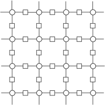
Figure 1: Part of the factor-graph for the two-dimensional Edwards-Anderson model on a square lattice. Circles represents variable nodes and squares represent interactions.

The factor-graph of model (1) might contain many short loops, which cause strong local correlations among the variable nodes. To better describe the correlations and fluctuations caused by short loops in the system, it is desirable to view the factor-graph as a union of different regions. Each region contains a set of variable nodes and function nodes. The variable nodes that appear in the same region are supposed to be strongly correlated and are treated with special care. More precisely, a region-graph $R$ is formed by regions $\{\alpha,\gamma,\mu,\ldots\}$ and the edges $\{(\alpha,\gamma),(\mu,\nu),\ldots\}$ between regions [12]. A region $\alpha$ contains some variable nodes and function nodes of the factor graph, it satisfies the condition that, if a function node $a\in\alpha$, then all the variable nodes connected to $a$ are in $\alpha$ (that is, $\partial a\subset\alpha$). The region concept is an extension of the cluster concept of the cluster variation method [10, 11]. The edges in a region-graph are directed. If there is an edge pointing from a region $\mu$ to another region $\nu$, then $\nu$ must be a subregion of $\mu$ (namely, if variable node $i\in\nu$, then $i\in\mu$, and if function node $a\in\nu$, then $a\in\mu$). If there is a directed path from region $\alpha$ to region $\gamma$, then we say that $\gamma<\alpha$ and $\alpha>\gamma$ (notice that if there is no directed path from $\alpha$ to $\gamma$, such an ordering relationship does not exist, even if $\gamma\subset\alpha$).

Each region $\alpha$ of the region-graph has a counting number $c_{\alpha}$ that is recursively determined by

$$c_{\alpha}=1-\sum\limits_{\{\gamma|\gamma\in R,\gamma>\alpha\}}c_{\gamma}.$$ (4)

Notice that $\sum_{\gamma\geq\alpha}c_{\gamma}=1$ for any region $\alpha\in R$, that is, each region is counted exactly once (see [12, 11]). The region-graph $R$ and its associated counting numbers are required to satisfy the following region-graph condition [12]: For any variable node $i$, the subgraph of $R$ formed by all the regions $\alpha$ containing $i$ and all the edges between these regions is connected; furthermore,

$$\sum\limits_{\{\alpha|i\in\alpha\}}c_{\alpha}=1,\quad\quad\sum\limits_{\{\alpha|a\in\alpha\}}c_{\alpha}=1.$$ (5)

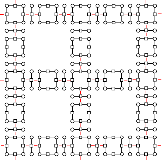
Figure 2: Part of a region-graph for the 2D Edwards-Anderson model, whose factor-graph is shown in figure 1. There are two types of regions, the square regions (containing four variable nodes and four function nodes) and the pair regions (containing two variable nodes and one function node). The red short lines represent the edges of the region-graph. Each square region has a counting number $c=1$, and each pair region has a counting number $c=-1$.

For the same factor-graph it is usually possible to construct many different region-graphs which all satisfy the region-graph condition. The factor-graph itself can be turned into the simplest region-graph with two types of regions (each small region is formed by a single variable node, and each large region is formed by a function node and all the connected variable nodes). Constructing an appropriate region-graph for a graphical model (1) is by no means a trivial issue, a lot of physical insights are needed here. We leave this construction problem as an open issue for future study, and simply assume a suitable region-graph $R$ for model (1) is ready for use. To give a simple example, we show in figure 2 part of a region-graph for the EA model (2) on a 2D square lattice.

Partition function expansion—Because of the region-graph condition (5), we can reformulate the partition function (3) as

$$Z(\beta)=\sum\limits_{\underline{x}}\prod\limits_{\alpha\in R}\biggl{[}\prod_{a\in\alpha}\psi_{a}(\underline{x}_{\partial a})\biggr{]}^{c_{\alpha}}.$$ (6)

For each region $\alpha$ we define its configuration as $\underline{x}_{\alpha}\equiv\{x_{i}^{\alpha}|i\in\alpha\}$, where $x_{i}^{\alpha}$ is the state of node $i$ in $\alpha$. For a function node $a$ in region $\alpha$, the variable states at its neighborhood is then denoted as $\underline{x}_{\partial a}^{\alpha}$, with $\underline{x}_{\partial a}^{\alpha}\equiv\{x_{i}^{\alpha}|i\in\partial a\}$. The Boltzmann factor for region $\alpha$ is denoted as $\Psi_{\alpha}(\underline{x}_{\alpha})\equiv\prod_{a\in\alpha}\psi_{a}^{c_{\alpha}}(\underline{x}_{\partial a}^{\alpha})$.

A variable node $i$ may belong to two or more regions (say $\alpha,\gamma,\ldots$). If this is the case, we regard the states $x_{i}^{\alpha},x_{i}^{\gamma},\ldots$ of node $i$ in the different regions as different variables. With these auxiliary states $\{\underline{x}_{\alpha}|\alpha\in R\}$, we then have

$$Z(\beta) =\sum\limits_{\underline{x}}\sum\limits_{\{\underline{x}_{\alpha}\}}\prod\limits_{\alpha\in R}\Bigl{[}\Psi_{\alpha}(\underline{x}_{\alpha})\Bigr{]}\prod\limits_{\gamma\in R}\prod_{i\in\gamma}\delta(x_{i}^{\gamma},x_{i})$$ (7)

$$=\sum\limits_{\{\underline{x}_{\alpha}\}}\prod\limits_{\alpha\in R}\Bigl{[}\Psi_{\alpha}(\underline{x}_{\alpha})\Bigr{]}\prod_{(\mu,\nu)\in R}\biggl{[}\prod_{i\in\mu\cap\nu}\delta(x_{i}^{\mu},x_{i}^{\nu})\biggr{]},$$ (8)

where the Kronecker symbol $\delta(x,y)=1$ if $x=y$ and $\delta(x,y)=0$ otherwise. The equivalence of (8) and (7) is ensured by the region-graph condition that the subgraph induced by any variable node $i$ is connected. In (8), the product over all the edges $(\mu,\nu)$ of the region-graph $R$ makes sure that, the partition function $Z$ is contributed only by those region configurations for which each variable node $i$ takes the same state in all the different regions that contain $i$. These are the edge constraints on $R$. We notice that, if in $R$ there are two or more directed paths from a region $\alpha$ to another region $\gamma$, then some of the region-graph edge constraints are redundant in the sense that they can be removed from the edge product without affecting the equivalence of (8) and (7). It is desirable for a region-graph $R$ to be free of redundant edges. If some edges of $R$ are redundant, it should not be included in the edge product of (8). In what follows, for simplicity, we assume that the region-graph $R$ contains no redundant edges.

For each edge $(\mu,\nu)\in R$ we introduce two auxiliary probability distributions $p_{\mu\rightarrow\nu}(\underline{x}_{\nu\cap\mu})$ and $p_{\nu\rightarrow\mu}(\underline{x}_{\mu\cap\nu})$. They are at the moment arbitrary functions under the minimal constraints of being nonnegative and normalized. The state vector $\underline{x}_{\mu\cap\nu}$ is defined as $\underline{x}_{\mu\cap\nu}\equiv\{x_{i}^{\mu}|i\in\mu\cap\nu\}$, similarly $\underline{x}_{\nu\cap\mu}\equiv\{x_{i}^{\nu}|i\in\mu\cap\nu\}$. We then get the following formula of central importance

$$\quad\quad Z(\beta)=\sum\limits_{\{\underline{x}_{\alpha}\}}\prod\limits_{\alpha\in R}\biggl{[}\Psi_{\alpha}(\underline{x}_{\alpha})\prod_{\gamma\in\partial\alpha}p_{\gamma\rightarrow\alpha}(\underline{x}_{\alpha\cap\gamma})\biggr{]}\prod_{(\mu,\nu)\in R}\biggl{[}\frac{\prod_{i\in\mu\cap\nu}\delta(x_{i}^{\mu},x_{i}^{\nu})}{p_{\mu\rightarrow\nu}(\underline{x}_{\nu\cap\mu})p_{\nu\rightarrow\mu}(\underline{x}_{\mu\cap\nu})}\biggr{]},$$ (9)

where $\partial\alpha$ denotes the set of regions that are connected with region $\alpha$ by an edge. A loop series expression for the partition function (9) can be easily written down following [14]. The equilibrium free energy $F(\beta)\equiv-(1/\beta)\ln Z(\beta)$ of the system is expressed as

$$F(\beta)=F_{0}-\frac{1}{\beta}\ln\biggl{[}1+\sum\limits_{r_{loop}\subseteq R}L_{r_{loop}}\biggr{]},$$ (10)

where $r_{loop}$ denotes any subgraph that is free of dangling edges (each $\alpha\in r_{loop}$ is connected with at least two other regions of $r_{loop}$), and $L_{r_{loop}}$ is its correction contribution to the free energy. To ensure that any subgraph $r$ with at least one dangling edge has zero correction contribution, the auxiliary probability functions need to satisfy the following equation

$$\quad\quad p_{\mu\rightarrow\nu}(\underline{x}_{\nu\cap\mu})=B_{\mu\rightarrow\nu}(\{p_{\gamma\rightarrow\mu}\})\equiv\frac{\sum\limits_{\underline{x}_{\mu}}\prod\limits_{i\in\mu\cap\nu}\delta(x_{i}^{\mu},x_{i}^{\nu})\Psi_{\mu}(\underline{x}_{\mu})\prod\limits_{\gamma\in\partial\mu\backslash\nu}p_{\gamma\rightarrow\mu}(\underline{x}_{\mu\cap\gamma})}{\sum_{\underline{x}_{\mu}}\Psi_{\mu}(\underline{x}_{\mu})\prod_{\gamma\in\partial\mu\backslash\nu}p_{\gamma\rightarrow\mu}(\underline{x}_{\mu\cap\gamma})}.$$ (11)

This self-consistent equation is referred to as the region-graph belief-propagation (rgBP) equation.

The free energy $F_{0}$ in (10) is expressed as

$$F_{0}=\sum\limits_{\gamma\in R}f_{\gamma}-\sum\limits_{(\mu,\nu)\in R}f_{(\mu,\nu)},$$ (12)

with

$$f_{\gamma} \equiv-\frac{1}{\beta}\ln\biggl{[}\sum_{\underline{x}_{\gamma}}\Psi_{\gamma}(\underline{x}_{\gamma})\prod_{\alpha\in\partial\gamma}p_{\alpha\rightarrow\gamma}(\underline{x}_{\gamma\cap\alpha})\biggr{]},$$

$$f_{(\mu,\nu)} \equiv-\frac{1}{\beta}\ln\biggl{[}\sum_{\underline{x}_{\mu\cap\nu}}p_{\mu\rightarrow\nu}(\underline{x}_{\mu\cap\nu})p_{\nu\rightarrow\mu}(\underline{x}_{\mu\cap\nu})\biggr{]}.$$

The loop correction $L_{r}$ has the following expression

$$L_{r}=\sum\limits_{\{\underline{x}_{\gamma}|\gamma\in r\}}\prod\limits_{\gamma\in r}w_{\gamma}(\underline{x}_{\gamma})\prod_{(\mu,\nu)\in r}\Delta_{(\mu,\nu)},$$ (13)

with

$$\Delta_{(\mu,\nu)}=\frac{e^{-yf_{(\mu,\nu)}}\prod_{i\in\mu\cap\nu}\delta(x_{i}^{\mu},x_{i}^{\nu})}{p_{\mu\rightarrow\nu}(\underline{x}_{\nu\cap\mu})p_{\nu\rightarrow\mu}(\underline{x}_{\mu\cap\nu})}-1,$$

$$w_{\gamma}(\underline{x}_{\gamma})=\frac{\Psi_{\gamma}(\underline{x}_{\gamma})\prod_{\alpha\in\partial\gamma}p_{\alpha\rightarrow\gamma}(\underline{x}_{\gamma\cap\alpha})}{\sum_{\underline{x}_{\gamma}}\Psi_{\gamma}(\underline{x}_{\gamma})\prod_{\alpha\in\partial\gamma}p_{\alpha\rightarrow\gamma}(\underline{x}_{\gamma\cap\alpha})}.$$

At a fixed point of the rgBP equation (11), $F_{0}$ gives an approximate expression for the true free energy of the system, when all the loop corrections in (10) are neglected. A nice property of $F_{0}$ is that, when viewed as a functional of the probability functions $\{p_{\mu\rightarrow\nu},p_{\nu\rightarrow\mu}\}$, the first variation of $F_{0}$ vanishes at a fixed point of (11). In other words, $F_{0}$ attains its extremal value at a rgBP fixed point. Because of this extremal property, we regard a fixed point of (11) as a macroscopic state of the model (1), with extremal free energy value $F_{0}$. Using the counting number expression (4), we can re-express $F_{0}$ as

$$F_{0} = \sum\limits_{\gamma\in R}\Bigl{[}c_{\gamma}+\sum_{\alpha>\gamma}c_{\alpha}\Bigr{]}f_{\gamma}-\sum\limits_{(\mu\rightarrow\nu)}\Bigl{[}c_{\mu}+\sum_{\alpha>\mu}c_{\alpha}\Bigr{]}f_{(\mu,\nu)}$$ (14)

$$= \sum\limits_{\alpha\in R}c_{\alpha}\tilde{f}_{\alpha},$$

where $(\mu\rightarrow\nu)$ denotes a directed edge of $R$ from region $\mu$ to region $\nu$, and $\tilde{f}_{\alpha}$ is the free energy of region $\alpha$ as expressed by

$$\tilde{f}_{\alpha}=\sum\limits_{\gamma\leq\alpha}f_{\gamma}-\sum\limits_{(\mu,\nu):\mu\leq\alpha,\nu\leq\alpha}f_{(\mu,\nu)}.$$ (15)

Notice (14) has the same formal expression as the region-graph variational free energy expression $F_{RG}$ of [12]. But $F_{0}$ and $F_{RG}$ in general may not be equivalent.

The statistical mechanics description of a single macroscopic state of model (1) is composed of (10) and (11). It can be regarded as forming a replica-symmetric spin-glass theory in the region-graph representation. If the typical length of the loops of the region-graph is long enough, since each $\Delta_{(\mu,\nu)}$ in the product of (13) has zero mean value under the probability measures $\{w_{\gamma}(\underline{x}_{\gamma})\}$, the loop correction contributions to the free energy might be negligible within each macroscopic state of the system.

For the region-graph shown in figure 2 representing the the square-lattice EA model, the explicit form of the rgBP equation (11) can be easily obtained. We have applied the rgBP equation on single instances of the 2D EA model and obtained quite satisfactory results (will be reported in a full paper). In the case that all the coupling constants $J_{ij}\equiv J>0$ (the Ising model), the rgBP equation predicts a phase-transition from the paramagnetic phase to the ferromagnetic phase at a critical temperature value $T=2.65635J$. This value is lower than the value of $T=2.8854J$ as obtained by the Bethe-Peierls approximation, but still higher than the exact critical temperature $T=2.2692J$. Further improvements on the critical temperature prediction should be achievable by working on region-graphs with larger regions.

Grand partition function expansion—For graphical models with strong disorder and frustration, very probably the rgBP equation (11) has multiple fixed points at low enough temperatures. This situation corresponds to the existence of multiple low-temperature macroscopic states $s$ of the model (1), each of which is characterized by an extremal free energy value $F_{0}^{(s)}$. A full understanding of the equilibrium property of the system then requires a quantitative description of the free energy landscape at the level of macroscopic states. For this purpose, we follow [14] (see also [4, 5]) and introduce a grand partition function $\Xi(y;\beta)$

$$\quad\quad\Xi(y;\beta) \equiv \sum_{s}e^{-yF_{0}^{(s)}}$$ (16)

$$= \prod\limits_{(\mu,\nu)\in R}\int{\rm D}p_{\mu\rightarrow\nu}\int{\rm D}p_{\nu\rightarrow\mu}\delta\Bigl{(}p_{\mu\rightarrow\nu}-B_{\mu\rightarrow\nu}\Bigr{)}\delta\Bigl{(}p_{\nu\rightarrow\mu}-B_{\nu\rightarrow\mu}\Bigr{)}e^{-yF_{0}}.$$

Because of the Dirac delta functions, only the rgBP fixed points contribute to the grand partition function. The parameter $y$ is the inverse temperature at the level of macroscopic states. For each edge $(\mu,\nu)$ of the region-graph we introduce two auxiliary probability functions $P_{\mu\rightarrow\nu}(p_{\mu\rightarrow\nu})$ and $P_{\nu\rightarrow\mu}(p_{\nu\rightarrow\mu})$ and rewrite (16) as

$$\quad\Xi(y;\beta)=$$

$$\quad\quad\prod\limits_{\alpha\in R}\biggl{[}\prod_{\gamma\in\partial\alpha}\int{\rm D}p_{\gamma\rightarrow\alpha}P_{\gamma\rightarrow\alpha}(p_{\gamma\rightarrow\alpha})e^{-yf_{\alpha}}\biggr{]}\prod\limits_{(\mu,\nu)\in R}\biggl{[}\frac{\delta(p_{\mu\rightarrow\nu}-B_{\mu\rightarrow\nu})\delta(p_{\nu\rightarrow\mu}-B_{\nu\rightarrow\mu})}{e^{-yf_{(\mu,\nu)}}P_{\mu\rightarrow\nu}(p_{\mu\rightarrow\nu})P_{\nu\rightarrow\mu}(p_{\nu\rightarrow\mu})}\biggr{]}.$$ (17)

We can then follow [14] and obtain a loop series for the expression (17). The grand free energy of the system $G(y;\beta)\equiv(-1/y)\ln\Xi(y;\beta)$ is written as

$$G(y;\beta)=G_{0}-\frac{1}{\beta}\ln\biggl{[}1+\sum\limits_{r_{loop}\subseteq R}L_{r_{loop}}^{(1)}\biggr{]},$$ (18)

where the leading term $G_{0}$ has the expression

$$G_{0}(y;\beta)=\sum\limits_{\gamma\in R}g_{\gamma}-\sum\limits_{(\mu,\nu)\in R}g_{(\mu,\nu)},$$ (19)

with

$$g_{\gamma} \equiv-\frac{1}{y}\ln\biggl{[}\prod_{\alpha\in\partial\gamma}\int{\rm D}p_{\alpha\rightarrow\gamma}P_{\alpha\rightarrow\gamma}(p_{\alpha\rightarrow\gamma})e^{-yf_{\gamma}}\biggr{]},$$

$$g_{(\mu,\nu)} \equiv-\frac{1}{y}\ln\biggl{[}\int\int{\rm D}p_{\mu\rightarrow\nu}{\rm D}p_{\nu\rightarrow\mu}P_{\mu\rightarrow\nu}(p_{\mu\rightarrow\nu})P_{\nu\rightarrow\mu}(p_{\nu\rightarrow\mu})e^{-yf_{(\mu,\nu)}}\biggr{]}.$$

The correction contribution $L_{r}^{(1)}$ of a subgraph to the grand free energy has a similar expression as (13) [14]. To ensure that any subgraph with at least one dangling edge has vanishing correction contribution to the grand free energy, each probability function $P_{\mu\rightarrow\nu}(p_{\mu\rightarrow\nu})$ needs to satisfy the following equation

$$P_{\mu\rightarrow\nu}(p_{\mu\rightarrow\nu})=S_{\mu\rightarrow\nu}[\{P_{\gamma\rightarrow\mu}\}]\equiv\frac{\prod\limits_{\gamma\in\partial\mu\backslash\nu}\int{\rm D}p_{\gamma\rightarrow\mu}P_{\gamma\rightarrow\mu}(p_{\gamma\rightarrow\mu})e^{-yf_{\mu\rightarrow\nu}}\delta\bigl{(}p_{\mu\rightarrow\nu}-B_{\mu\rightarrow\nu}\bigr{)}}{\prod_{\gamma\in\partial\mu\backslash\nu}\int{\rm D}p_{\gamma\rightarrow\mu}P_{\gamma\rightarrow\mu}(p_{\gamma\rightarrow\mu})e^{-yf_{\mu\rightarrow\nu}}},$$ (20)

where

$$f_{\mu\rightarrow\nu}\equiv-\frac{1}{\beta}\ln\biggl{[}\sum_{\underline{x}_{\mu}}\Psi_{\mu}(\underline{x}_{\mu})\prod_{\gamma\in\partial\mu\backslash\nu}p_{\gamma\rightarrow\mu}(\underline{x}_{\mu\cap\gamma})\biggr{]}.$$

Equation (20) is called the region-graph survey-propagation (rgSP) equation. If we neglect loop correction contributions, $G_{0}$ then gives an approximate expression for the true grand free energy. By knowing the grand free energy values at different inverse temperatures $y$, we can then calculate the number $\exp[N\Sigma(f)]$ of macroscopic states with given extremal free energy density $f\equiv F_{0}/N$ [5, 14]. $\Sigma(f)$ is called the complexity function in spin-glass literature [2]. It gives a quantitative description of the free energy landscape of the $F_{0}$ functional (12). Notice that $G_{0}$ can again be viewed as a functional of the probability distributions $\{P_{\mu\rightarrow\nu},P_{\nu\rightarrow\mu}\}$. It is easy to check that the first variation of $G_{0}$ vanishes at a fixed point of (20), suggesting that each rgSP fixed point corresponds to an extremal value of $G_{0}$.

The statistical mechanics description of the model (1) at the level of macroscopic states is composed of (18) and (20). This description can be regarded as the first-step replica-symmetry-breaking (1RSB) spin-glass theory in the region-graph representation.

If the free energy functional $G_{0}$ has multiple extremal values, then a higher-level partition function needs to be defined similar to (16), and the free energy landscape of $G_{0}$ will then be described by a higher-level message-passing equation. This hierarchy of partition function expansions can be continued to even higher levels if necessary, leading to a mathematical theory that can be regarded as the full-step RSB spin-glass theory in the region-graph representation.

Conclusion and discussions—For a general graphical model (1) represented through a region-graph, a statistical mechanics theory was rigorously derived in this work from the mathematical framework of partition function expansion [14]. The obtained free energy expressions and message-passing equations are exact in the sense the no assumptions nor approximations were made during the theoretical construction. This theory is most suitable for studying finite-dimensional models which are full of short loops and strong local correlations. The theory reduces to that of [14] in the special case of the region-graph being a factor-graph.

Yedidia and co-authors [12] constructed a variational free energy based on some heuristic arguments and consistency requirements, and they then obtained several sets of generalized belief-propagation equations. The starting point of the variational approaches of [12] and [10, 11] is the non-equilibrium Gibbs free energy functional, while our starting point is the equilibrium partition function. Because of this qualitative difference, the free energy expression $F_{0}$ in general may not be equivalent to the variational free energy expression of [12]. In an accompanying full paper we will investigate this issue more systematically. A comparison between the rgBP (11) and the generalized belief-propagation schemes of [12] will also be made. The possible links between our approach and the replica cluster variation method of [13] will also be thoroughly discussed in the accompanying paper.

A distributed algorithm of message-passing can be implemented on single finite-dimensional graphical models. To be efficient, a suitable representation for the probability distributions $p_{\mu\rightarrow\nu}(\underline{x}_{\nu\cap\mu})$ and $P_{\mu\rightarrow\nu}(p_{\mu\rightarrow\nu})$ should be worked out. For the 2D square-lattice EA model (2), if we represent it by a region-graph shown in figure 2, the rgBP equation can be easily implemented. Systematic numerical results on the 2D and 3D EA model with bimodal coupling constants will be reported in another paper.

References

References

- [1] M. Mézard, G. Parisi, and M. A. Virasoro. Spin Glass Theory and Beyond. World Scientific, Singapore, 1987.
- [2] M. Mézard and A. Montanari. Information, Physics, and Computation. Oxford Univ. Press, New York, 2009.
- [3] M. Mézard, G. Parisi, and M. A. Virasoro. SK model: the replica solution without replicas. Europhys. Lett., 1:77–82, 1986.
- [4] R. Monasson. Structural glass transition and the entropy of the metastable states. Phys. Rev. Lett., 75:2847–2850, 1995.
- [5] M. Mézard and G. Parisi. The bethe lattice spin glass revisited. Eur. Phys. J. B, 20:217–233, 2001.
- [6] M. Mézard, G. Parisi, and R. Zecchina. Analytic and algorithmic solution of random satisfiability problems. Science, 297:812–815, 2002.
- [7] F. Krzakala, A. Montanari, F. Ricci-Tersenghi, G. Semerjian, and L. Zdeborova. Gibbs states and the set of solutions of random constraint satisfaction problems. Proc. Natl. Acad. Sci. USA, 104:10318–10323, 2007.
- [8] S. F. Edwards and P. W. Anderson. Theory of spin glasses. J. Phys. F: Met. Phys., 5:965–974, 1975.
- [9] F. Belletti, M. Cotallo, A. Cruz, L. A. Fernandez, A. Gordillo-Guerrero, M. Guidetti, A. Maiorano, F. Mantovani, E. Marinari, V. Martin-Mayor, A. Muñoz Sudupe, D. Navarro, G. Parisi, S. Perez-Gaviro, J. J. Ruiz-Lorenzo, S. F. Schifano, D. Sciretti, A. Tarancon, R. Tripiccione, J. L. Velasco, and D. Yllanes. Nonequilibrium spin-glass dynamics from picoseconds to a tenth of a second. Phys. Rev. Lett., 101:157201, 2008.
- [10] R. Kikuchi. A theory of cooperative phenomena. Phys. Rev., 81:988–1003, 1951.
- [11] G. An. A note on the cluster variation method. J. Stat. Phys., 52:727–734, 1988.
- [12] J. S. Yedidia, W. T. Freeman, and Y. Weiss. Constructing free-energy approximations and generalized belief-propagation algorithms. IEEE Trans. Inf. Theory, 51:2282–2312, 2005.
- [13] T. Rizzo, A. Lage-Castellanos, R. Mulet, and F. Ricci-Tersenghi. Replica cluster variational method. J. Stat. Phys., 139:375–416, 2010.
- [14] J.-Q. Xiao and H. Zhou. Partition function loop series for a general graphical model: free-energy corrections and message-passing equations. J. Phys. A: Math. Theor., 44:425001, 2011.
- [15] M. Chertkov and V. Y. Chernyak. Loop series for discrete statistical models on graphs. J. Stat. Mech.: Theor. Exp., P06009, 2006.
- [16] F. R. Kschischang, B. J. Frey, and H.-A. Loeliger. Factor graphs and the sum-product algorithm. IEEE Trans. Inf. Theory, 47:498–519, 2001.