Non-Gaussian Scale Space Filtering with 2$\times$2 Matrix of Linear Filters

Abstract

Construction of a scale space with a convolution filter has been studied extensively in the past. It has been proven that the only convolution kernel that satisfies the scale space requirements is a Gaussian type. In this paper, we consider a matrix of convolution filters introduced in [1] as a building kernel for a scale space, and shows that we can construct a non-Gaussian scale space with a $2\times 2$ matrix of filters. The paper derives sufficient conditions for the matrix of filters for being a scale space kernel, and present some numerical demonstrations.

1 Introduction

Linear scale-space representations have been applied to many signal and image processing problems[2][3], in which an optimum amount of smoothing cannot be determined in advance. The linear scale space smoothing iteratively applies a linear diffusion operator to the signal until an appropriate amount of smoothing is introduced.

Recently, we proposed a new approach to signal smoothing [1], which is linear, diffusion-like, but possesses different frequency characteristics from the linear diffusion operator; as the number of iteration increases, our filter develops a sharper cut-off but retains the bandwidth much longer than the linear diffusion. The filter was designed from a geometrical perspective and called Elastic Quadratic Wire (EQW). We can consider EQW smoothing as applications of linear filters (in particular circular convolution filters) to the signal and its auxiliary extensions in a computational structure similar to a linear transformation by a $3\times 3$ matrix where each component is one of the convolution filters.

Our goal is to understand the frequency characteristics of EQW and derive general requirements on the filter coefficients to meet the scale space criteria[4][3]. It has been shown that the only convolution kernel that satisfies the scale space requirements is a Gaussian type for the continuous time space [5][4][6] and the modified Bessel functions of integer order for the discrete time space. The latter approaches the Gaussian kernel as the length of the filter increases. In this paper, instead of considering a convolution filter, we consider a matrix of convolution filters employed for the EQW smoothing. In particular, instead of $3\times 3$ matrix of filters as in the original EQW, we study a $2\times 2$ form. Although smaller in size, the configuration retains some of intrinsic characteristics of the original EQW and allows us to characterize the frequency response algebraically. We will extend the results in the future for larger and more general configurations.

2 Background

We consider the following linear system.

$$\left(\begin{array}[]{c}\mathbf{x}_{1}^{[l+1]}\\ \mathbf{x}_{2}^{[l+1]}\\ \vdots\\ \mathbf{x}_{P}^{[l+1]}\end{array}\right)=(1-t)\left(\begin{array}[]{c}\mathbf{x}_{1}^{[l]}\\ \mathbf{x}_{2}^{[l]}\\ \vdots\\ \mathbf{x}_{P}^{[l]}\end{array}\right)+t\left(\begin{array}[]{c}\sum_{s=1}^{P}\mathbf{f}_{1s}\ast\mathbf{x}_{s}^{[l]}\\ \sum_{s=1}^{P}\mathbf{f}_{2s}\ast\mathbf{x}_{s}^{[l]}\\ \vdots\\ \sum_{s=1}^{P}\mathbf{f}_{Ps}\ast\mathbf{x}_{s}^{[l]}\\ \end{array}\right)$$ (1)

where $P$ is the order of the system, $\mathbf{x}_{s}^{[\cdot]}$ ($1\leq s\leq P$) are discrete signals of length $N$ in which the number inside $[~{}]$ indicates the iteration number, $t\geq 0$ is a scale parameter, $\mathbf{f}_{rs}$ ($1\leq r,s\leq P$) are linear filters, and $\ast$ is a circular convolution operator. The operator is applied iteratively, and (1) implies that the outputs of $l$th iteration becomes the inputs to the $l+1$st iteration. We call this computational structure a matrix of filters, as the filters can be arranged in a $P\times P$ matrix form and the operation can be conveniently viewed as a multiplication (defined as in (1)) of the matrix with the input signals. Figure 1 shows two stages of a $P\times P$ matrix of filters. Note that the computation at each stage is identical.

Figure 1: A schematic of a $P\times P$ matrix of linear filters. A rectangle with $*\mathbf{f}_{rs}$ is a linear filter whose impulse response is $\mathbf{f}_{rs}$. A circle with $+$ receives $P$ inputs and adds them at every cycle.

2.1 Equivalent filter

Let $\mathbf{M}_{rs}$ be a $N$ by $N$ circulant matrix that implements the linear filter of $\mathbf{f}_{rs}$. Let

$$\mathbf{M}=\left(\begin{array}[]{ccc}\mathbf{M}_{11}&\ldots&\mathbf{M}_{1P}\\ \vdots&\ddots&\vdots\\ \mathbf{M}_{P1}&\ldots&\mathbf{M}_{PP}\\ \end{array}\right).$$ (2)

Write the $l$th power of $\mathbf{M}$ as

$$\mathbf{M}^{l}=\left(\begin{array}[]{ccc}\mathbf{M}_{11}^{[l]}&\ldots&\mathbf{M}_{1P}^{[l]}\\ \vdots&\ddots&\vdots\\ \mathbf{M}_{P1}^{[l]}&\ldots&\mathbf{M}_{PP}^{[l]}\\ \end{array}\right).$$ (3)

Then, the signal at $l$th iteration can be expressed in terms of the initial signals ($\mathbf{x}_{1}^{[0]}\ldots\mathbf{x}_{P}^{[0]}$) by

$$\left(\begin{array}[]{c}\mathbf{x}_{1}^{[l]}\\ \vdots\\ \mathbf{x}_{P}^{[l]}\\ \end{array}\right)=\left(\begin{array}[]{ccc}\mathbf{M}_{11}^{[l]}&\ldots&\mathbf{M}_{1P}^{[l]}\\ \vdots&\ddots&\vdots\\ \mathbf{M}_{P1}^{[l]}&\ldots&\mathbf{M}_{PP}^{[l]}\\ \end{array}\right)\left(\begin{array}[]{c}\mathbf{x}_{1}^{[0]}\\ \vdots\\ \mathbf{x}_{P}^{[0]}\\ \end{array}\right).$$ (4)

Now we designate $\mathbf{x}_{1}$ as the primary signal and $\mathbf{x}_{s}$ ($s>1$) as auxiliary ones. Initially, all auxiliary signals are set to zero. Then, $\mathbf{x}_{1}^{[0]}$ and $\mathbf{M}_{11}^{[l]}$ determine $\mathbf{x}_{1}^{[l]}$, the primary signal at the $l$th iteration. $\mathbf{M}_{11}^{[l]}$ is also circulant as circulant matrices are closed under addition and multiplication. Therefore, it implements circular convolution of a filter denoted as $\mathbf{f}_{11}^{[l]}$, which we call an equivalent filter at $l$th iteration. The equivalent filter transforms $\mathbf{x}_{1}^{[0]}$ to $\mathbf{x}_{1}^{[l]}$.

2.2 Eigen-decomposition

Define

$$\mathbf{B}_{i}=\left(\begin{array}[]{ccc}\mathbf{f}_{11}(i)&\ldots&\mathbf{f}_{1P}(i)\\ \vdots&\ddots&\vdots\\ \mathbf{f}_{P1}(i)&\ldots&\mathbf{f}_{PP}(i)\end{array}\right)$$ (5)

where $\mathbf{f}_{rs}(i)$ denotes the $i$th coefficient of $\mathbf{f}_{rs}$ and

$$\mathbf{H}(\rho^{k})=\sum_{i=0}^{N-1}\mathbf{B}_{i}\rho^{ik}$$ (6)

where $\rho=e^{j2\pi/N}$. Then, the eigenvalues of $\mathbf{H}\left(\rho^{k}\right)$ ($0\leq k\leq N-1$) are eigenvalues of $\mathbf{M}$. For each $k$, there are P eigenvalues. Thus, there are total of $PN$ eigenvalues for $\mathbf{M}$ with possible repetition. Let $\lambda_{i}^{k}$ ($i\in\left\{1,\ldots P\right\}$) be an eigenvalue of $\mathbf{H}(\rho^{k})$ and $\mathbf{v}_{i}^{k}$ be the corresponding eigenvector. Let $\mathbf{r}^{k}=\left[\rho^{0}~{}\rho^{k}\cdots\rho^{k(N-1)}\right]^{T}$ (with the superscript $T$ denotes transposition). Then $\mathbf{v}_{i}^{k}\bigotimes\mathbf{r}(\rho^{k})$ where $\bigotimes$ denotes the Kronecker product is an eigenvector of $\mathbf{M}$.

Let $\mathbf{V}^{k}=\left[\mathbf{v}_{1}^{k}\ldots\mathbf{v}_{P}^{k}\right]$, $\mathbf{g}^{k}$ be the first row of $\mathbf{V}^{k}$, and $\tilde{\mathbf{g}}^{k}$ be the first column of $\left(\mathbf{V}^{k}\right)^{-1}$. Thus,

$$\mathbf{g}^{k}\cdot\tilde{\mathbf{g}}^{k}=1.$$ (7)

Let $\mathbf{D}_{i}$ ($i\in\left\{1\ldots P\right\}$) be an $N$ by $N$ diagonal matrix where $k$th diagonal component is $\lambda_{i}^{k}$ and $\mathbf{G}_{i}$ be another $N$ by $N$ diagonal matrix where $k$th diagonal component is $\mu_{i}^{k}=\mathbf{g}^{k}(i)\tilde{\mathbf{g}}^{k}(i)$. Note that $\mathbf{g}^{k}(i)$ denotes the $i$th component of $\mathbf{g}^{k}$. We call $\mu_{i}^{k}$ mixing coefficients, and

$$\sum_{i}\mu_{i}^{k}=1,$$ (8)

for all $0\leq k\leq N-1$ due to (7).

Then, $\mathbf{M}_{11}^{[l]}$ can be decomposed by

$$\mathbf{M}_{11}^{[l]}=\mathbf{W}\sum_{i=1}^{P}\mathbf{D}_{i}^{l}\mathbf{G}_{i}\mathbf{W}^{T}$$ (9)

where $\mathbf{W}$ is the $N$ by $N$ discrete Fourier transformation matrix and $W_{rs}=\rho^{rs}=e^{j2\pi rs/N}$. Hence, $\sum_{i=1}^{P}\mathbf{D}_{i}^{l}\mathbf{G}_{i}$ gives the frequency response of the equivalent filter at $l$th iteration.

2.3 Scale-Space Filters

We are interested in incremental smoothing of signals with small size filters. In literature, the approach is often referred to as scale space filtering and plays an important role in many signal and image processing applications. To maximize the control of the smoothing, we limit the number of non-zero filter coefficients in $\mathbf{f}_{rs}$ to three, the smallest symmetric filter size that allows construction of scale space. Thus, we assume $\mathbf{B}_{i}=\mathbf{0}$ for $i\notin\left\{-1,0,1\right\}$. In this paper, we consider requirements on $\mathbf{f}_{rs}$ for a $2\times 2$ matrix of filters so that its equivalent filter satisfies conditions for a scale space filter.

We impose the following conditions on equivalent filters.

1. Real frequency response: $\mathbf{f}_{11}^{[l]}$ is symmetric. In other words, the Fourier transform of the equivalent filter is real.

2. Positive response: Its frequency response is non-negative at every frequency component.

3. Unimodal response: Its frequency response is unimodal with the peak at the frequency 0.

4. Consistent reduction response: Each frequency component is non-increasing with respect to the iteration number.

5. Normalized response: The DC component of the Fourier transform is 1.

6. Equivalence to linear diffusion: It can be reduced to a common linear diffusion operator when the auxiliary signals are fixed at zero.

The first requirement prevents any phase distortion after the smoothing. The second through fourth requirements prevent any new local minimum or local maximum from forming as the result of smoothing, and are considered essential for scale space representations. Note that the fourth requirement is trivially satisfied for a conventional scale space filtering when the second requirement is satisfied. That is not the case for the matrix of filter based construction. The fifth requirement preserves the mean value of the signal. The equivalent to linear diffusion requirement states that the system without contributions from the auxiliary signal will result in linear diffusion. An iteration formula for the linear diffusion is [3]

$$\mathbf{x}_{1}^{k+1}=\left(1-2t\right)\mathbf{x}_{1}^{k}+t\left(z\mathbf{x}_{1}^{k}+z^{-1}\mathbf{x}_{1}^{k}\right).$$ (10)

where $z$ and $z^{-1}$ shift signals by one to the left and right, respectively, and $t\in\left[0,1/4\right]$.

3 Formulation

We introduce notations specific to the case of $2\times 2$ matrix of filters. To reduce the amount of arabic subscripts, we use $\mathbf{x}$ instead of $\mathbf{x}_{1}$ as the primary signal and $\mathbf{a}$ for the sole auxiliary signal, and write the processing of the $2\times 2$ matrix of filters as

$$\left(\begin{array}[]{c}\mathbf{x}^{[l+1]}\\ \mathbf{a}^{[l+1]}\end{array}\right)=\left(\begin{array}[]{c}\mathbf{x}^{[l]}\\ \mathbf{a}^{[l]}\end{array}\right)+t\left(\begin{array}[]{c}\mathbf{f}_{xx}\ast\mathbf{x}^{[l]}+\mathbf{f}_{xa}\ast\mathbf{a}^{[l]}\\ \mathbf{f}_{xa}\ast\mathbf{x}^{[l]}+\mathbf{f}_{aa}\ast\mathbf{a}^{[l]}\\ \end{array}\right).$$ (11)

Each convolution filters have at most three non-zero coefficients. Thus, we write them $\mathbf{f}_{\ast\ast}=[\alpha_{\ast\ast}~{}\beta_{\ast\ast}~{}\gamma_{\ast\ast}]$ with one tap delay so that $\beta_{\ast\ast}$ is the center of the filter. (Replace $\ast\ast$ with $xx$, $xa$, $ax$, or $aa$.)

Note that $k\in[0,N-1]$ where $N$ is the length of the input signal. Thus, as $N\rightarrow\infty$, $\rho^{k}$ covers all roots of unity. Since we want to derive design requirements for any signal length, we treat all quantities as functions of $\rho=\left\{z\in\mathbb{C}||z|=1\right\}$ or equivalently $\theta=\angle\rho\in[-\pi,\pi]$. This allows us to generalize our discussion and eliminate the superscript $k$ from expressions.

With these notations, eigenvalues of $\mathbf{B}$ are

$$\lambda_{1}(\rho)=\frac{\sigma_{xx}(\rho)+\sigma_{aa}(\rho)-\sqrt{\Delta(\rho)}}{2}$$ (12)

$$\lambda_{2}(\rho)=\frac{\sigma_{xx}(\rho)+\sigma_{aa}(\rho)+\sqrt{\Delta(\rho)}}{2},$$ (13)

and mixing coefficients are

$$\mu_{1}(\rho)=-\frac{\sigma_{xx}(\rho)-\sigma_{aa}(\rho)}{2\sqrt{\Delta(\rho)}}+\frac{1}{2}$$ (15)

$$\mu_{2}(\rho)=\frac{\sigma_{xx}(\rho)-\sigma_{aa}(\rho)}{2\sqrt{\Delta(\rho)}}+\frac{1}{2}$$ (16)

where

$$\sigma_{\ast\ast}(\rho)=\delta_{\ast\ast}(\rho)+t\left(\alpha_{\ast\ast}\rho^{-1}+\beta_{\ast\ast}+\gamma_{\ast\ast}\rho\right)$$ (17)

$$\Delta(\rho)=\left(\sigma_{xx}(\rho)-\sigma_{aa}(\rho)\right)^{2}+4\sigma_{ax}(\rho)\sigma_{xa}(\rho).$$ (18)

with $\delta_{rs}$ being the Kronecker’s delta function (1 when $r=s$ and 0 otherwise). Note that in (15) and (16), we are assuming that the eigenvalues are distinct (or $\Delta\neq 0$). When $\lambda_{1}=\lambda_{2}$, the mixing coefficients are arbitrary, and we set $\mu_{1}=\mu_{2}=1/2$.

Note that the above expressions are all functions of $\rho$ (or equivalently $\theta$). However, for brevity, we omit the variable in their expressions unless we are evaluating them at a particular $\rho$.

The frequency response of the equivalent filter at $l$th iteration is

$$F^{l}=D_{1}^{l}G_{1}+D_{2}^{l}G_{2}=$$

$$\mu_{1}\left(\frac{\sigma_{xx}+\sigma_{aa}-\sqrt{\Delta}}{2}\right)^{l}+\mu_{2}\left(\frac{\sigma_{xx}+\sigma_{aa}+\sqrt{\Delta}}{2}\right)^{l}.$$ (19)

4 Filter Requirements

In this section, we derive a sufficient condition for a $2\times 2$ matrix of filters to satisfy the scale space requirements. We first use necessary conditions to simplify the formulae of the individual filters. We then use the simplified formulae to derive sufficient conditions on the design parameters.

Theorem 4.1

Necessary conditions for a $2\times 2$ matrix of filters being a scale space filter are

$$\sigma_{xx}=\left(1-2t\right)+2t\cos\theta$$ (20)

$$\sigma_{aa}=\left(1-2bt\right)+2tc\cos\theta$$ (21)

$$\sigma_{xa}\sigma_{ax}=-4t^{2}d\sin^{2}\theta$$ (22)

where $b,c,d\in\mathbb{R}$.

Proof

$F^{l}$ at the first three iterations ($l=1,2,3$) are

$$F^{1}=\sigma_{xx},$$ (23)

$$F^{2}=\left(\sigma_{xx}\right)^{2}+\sigma_{xa}\sigma_{ax},$$ (24)

$$F^{3}=\left(\sigma_{xx}\right)^{3}+2\sigma_{xx}\sigma_{xa}\sigma_{ax}+\sigma_{aa}\sigma_{xa}\sigma_{ax}.$$ (25)

Since they have to be real according to the real frequency response requirement, $\sigma_{xx}$, $\sigma_{ax}\sigma_{xa}$ and $\sigma_{aa}$ have to be real. $\sigma_{xx}$ is real for any $k$ if and only if $\alpha_{xx}=\gamma_{xx}$ or $\mathbf{f}_{xx}$ is symmetric. $\sigma_{aa}$ is real for any $k$ if and only if $\alpha_{aa}=\gamma_{aa}$ or $\mathbf{f}_{aa}$ is symmetric. $\sigma_{ax}\sigma_{xa}$ is real for any $k$ if and only if either both $\sigma_{ax}$ and $\sigma_{xa}$ are real or both are imaginary. Thus, $\mathbf{f}_{ax}$ and $\mathbf{f}_{xa}$ are either both symmetric or anti-symmetric. Below, we show that either way, we will get the same condition for $\sigma_{ax}\sigma_{xa}$. Now, let’s introduce constraints derived from other requirements.

Due to the equivalence to linear diffusion requirement, we set $\alpha_{xx}=\gamma_{xx}=1$ and $\beta_{xx}=-2$, which gives

$$\sigma_{xx}=(1-2t)+2t\cos\theta.$$ (26)

For the normalized response requirement, the frequency response at $\theta=0$ has to be 1 for all $l$. Thus, $F^{1}(\theta=0)=F^{2}(\theta=0)=1$ has to be true. This gives $\sigma_{xx}(\theta=0)=1$ and $\sigma_{xa}(\theta=0)\sigma_{ax}(\theta=0)=0$. The former is satisfied with (26). The latter gives

$$\left(\alpha_{xa}+\beta_{xa}+\gamma_{xa}\right)\left(\alpha_{ax}+\beta_{ax}+\gamma_{ax}\right)=0.$$ (27)

Due to the constant reduction and the positivity requirements, $0\leq F^{2}(\theta)\leq F^{1}(\theta)$ or $0\leq\sigma_{xx}^{2}+\sigma_{xa}\sigma_{ax}\leq\sigma_{xx}$ for any $t\in[0,~{}1/4]$. Consider $t=1/4$. Then, $\sigma_{xx}(\theta=\pi)=0$. Hence, we have

$$\sigma_{xa}(\pi)\sigma_{ax}(\pi)=\left(\beta_{xa}-\alpha_{xa}-\gamma_{xa}\right)\left(\beta_{ax}-\alpha_{ax}-\gamma_{ax}\right)=0.$$ (28)

Now, we investigate if $\mathbf{f}_{xa}$ and $\mathbf{f}_{ax}$ should be both symmetric or anti-symmetric. First, Assume both are symmetric. Thus, $\gamma_{xa}=\alpha_{xa}$ and $\gamma_{ax}=\alpha_{ax}$. Because of the symmetry of (27) and (28), we consider $\left(\alpha_{ax}+\beta_{ax}+\gamma_{ax}\right)=0$ and $\left(\beta_{xa}-\alpha_{xa}-\gamma_{xa}\right)=0$, and the derivation for the other case will be the same. We have $\alpha_{ax}=\gamma_{ax}=-\beta_{ax}/2$ and $\alpha_{xa}=\gamma_{xa}=\beta_{xa}/2$, and obtain

$$\sigma_{xa}\sigma_{ax}=t^{2}\beta_{xa}\beta_{ax}\left(1-\cos^{2}\theta\right)=t^{2}\beta_{xa}\beta_{ax}\sin^{2}\theta.\\$$ (29)

Next, assume that both $\mathbf{f}_{xa}$ and $\mathbf{f}_{ax}$ are anti-symmetric. Thus, $\gamma_{xa}=-\alpha_{xa}$, $\gamma_{ax}=-\alpha_{ax}$, and $\beta_{xa}=\beta_{ax}=0$. In this case, both (27) and (28) are satisfied. Furthermore,

$$\sigma_{xa}\sigma_{ax}=-4t^{2}\alpha_{xa}\alpha_{ax}\sin^{2}\theta.\\$$ (30)

Therefore, given symmetric version of $\mathbf{f}_{xa}$ and $\mathbf{f}_{ax}$, we can always find anti-symmetric counterpart that provides the same expression for $\sigma_{xa}\sigma_{ax}$, and vice verse.

Let $\beta_{aa}=b$ and $\alpha_{aa}=\gamma_{aa}=c$. Then, we have $\sigma_{aa}=\left(1-2bt\right)+2ct\cos\theta$. Let both $\mathbf{f}_{xa}$ and $\mathbf{f}_{ax}$ are anti-symmetric, and $\alpha_{ax}\alpha_{xa}=d$. Then, we obtain the necessary condition. $\Box$

We have found that all scale space filters can be expressed by (20), (21), and (22). There are three design parameters: $b$, $c$, and $d$. The next theorem provides requirements on these parameters.

Theorem 4.2

Sufficient conditions for a $2\times 2$ matrix of filters being a scale space filter are that they are in the forms of (20)-(22) and

$$0\leq b+c\leq 2,$$ (31)

$$-2d\leq b-c\geq-2d,$$ (32)

$$c(b-c)\geq 2d,$$ (33)

$$c^{2}-(2-b)c+2d\leq 0$$ (34)

Proof

We first derive constraints on the three parameters for each scale space requirement.

Real frequency response requirement:

Since $\sigma_{xx}$, $\sigma_{aa}$ and $\sigma_{xa}\sigma_{ax}$ are all real and consequently $\Delta$, $\mu_{1}$, $\mu_{2}$, $\lambda_{1}$, and $\lambda_{2}$ are all real, the real frequency response is satisfied.

Equivalence to linear diffusion requirement: The equivalence to linear diffusion requirement is satisfied with (20).

Normalized response requirement: At $\theta=0$, $\sigma_{xa}\sigma_{ax}=0$ and $\Delta=\left(\sigma_{xx}^{0}-\sigma_{aa}^{0}\right)^{2}$. If $\sigma_{xx}^{0}\geq\sigma_{aa}^{0}$, $\lambda_{1}=0$, $\lambda_{2}=1$, $\mu_{1}=0$, and $\mu_{2}=1$. Thus, $F^{l}\left(\theta=0\right)=1$ for all $l\geq 1$. If $\sigma_{xx}^{0}<\sigma_{aa}^{0}$, $\lambda_{1}=1$, $\lambda_{2}=0$, $\mu_{1}=1$, and $\mu_{2}=0$. Again, $F^{l}\left(\theta=0\right)=1$ for all $l\geq 1$. Therefore, the normalized response requirement is satisfied.

Positive response and consistent reduction requirements: For convenience, we treat the two requirements together. Let

$$\phi=\sigma_{xx}+\sigma_{aa},$$ (35)

$$\psi=\sigma_{xx}-\sigma_{aa}.$$ (36)

Then,

$$F^{l}=\frac{\sqrt{\Delta}-\psi}{2\sqrt{\Delta}}\left(\frac{\phi-\sqrt{\Delta}}{2}\right)^{l}+\frac{\sqrt{\Delta}+\psi}{2\sqrt{\Delta}}\left(\frac{\phi+\sqrt{\Delta}}{2}\right)^{l}.$$ (37)

The positive response requirement is satisfied if

$$\psi\leq\sqrt{\Delta}$$

$$\phi\geq\sqrt{\Delta},$$

and the consistent reduction requirement is satisfied if

$$\psi\leq\sqrt{\Delta}$$

$$\phi+\sqrt{\Delta}\leq 2.$$

Thus, both conditions are satisfied if

$$\psi\leq\sqrt{\Delta}$$ (38)

$$\sqrt{\Delta}\leq\phi\leq 2-\sqrt{\Delta}.$$ (39)

Since $\Delta=\left(\psi\right)^{2}-d\sin^{2}\theta$, (38) is satisfied for all $\theta$ if

$$d\leq 0.$$ (40)

With $\phi\leq 2-\sqrt{\Delta}$, we have

$$\Delta\leq\left(2-\phi\right)^{2},\phi\leq 2.$$ (41)

Now,

$$(2-\phi)^{2}-\Delta=16t^{2}\left(\left(c-d\right)w-\left(b+d\right)\right)\left(w-1\right)\geq 0$$ (42)

where $w=\cos\theta$. Since $-1\leq w\leq 1$, $w-1\leq 0$. Thus, (42) is satisfied if

$$\left(c-d\right)w-\left(b+d\right)\leq 0.$$ (43)

The above inequality holds if and only if it holds at $w=1$ and $w=-1$. Hence,

$$b-c\geq-2d$$ (44)

$$b+c\geq 0.$$ (45)

With $\sqrt{\Delta}\leq\phi$, we have $\sigma_{xx}\sigma_{aa}\geq\sigma_{xa}\sigma_{ax}$ or

$$(1-2t+2tw)(1-2tb+2tcw)\geq-4dt^{2}(1-w^{2}).$$ (46)

Define

$$\eta(t,w)=(1-2t+2tw)(1-2tb+2tcw)+4dt^{2}(1-w^{2})$$

$$=4(1-w)\left(b+d-(c-d)w\right)t^{2}-2\left(1+b-(1+c)w\right)t+1.$$

To show (46), we need to show $\eta(t,w)\geq 0$.

Before deriving sufficient conditions for $\eta(t,w)\geq 0$, we find two necessary conditions for (46). We then show that the two conditions together with (40), (44), and (45) form sufficient conditions for $\eta(t,w)\geq 0$.

The right hand side of (46)is non-negative with(37) and $1-2t+2tw\geq 0$ for $0\leq t\leq 1/4$ and $-1\leq w\leq 1$. Thus, it is necessary that $1-2tb+2tcw\geq 0$. By setting $t=1/4$ and $w=1$, we have

$$b-c\leq 2.$$ (47)

By setting $t=1/4$ and $w=-1$, we have

$$b+c\leq 2.$$ (48)

When $(1-w)\left(b+d-(c-d)w\right)=0$, $\eta(t,w)\geq 0$ because

$$\eta(t,1)=1-2(b-c)t\geq 1-(b-c)/2\geq 0$$

(using $t\leq 1/4$ and $b-c\leq 2$) and

$$\eta(t,-1)=1-2\left(2+(b+c)\right)t=1-4t\geq 0$$

(using $b+c=0$ derived from $b+d-(c-d)(-1)=0$ and $t\leq 1/4$), and $\eta(t,w)$ in this case is a linear function of $w$.

With $(1-w)\left(b+d-(c-d)w\right)\neq 0$, we have

$$\eta(t,w)=4(1-w)\left(b+d-(c-d)w\right)\left(t-\frac{\left(1+b-(1+c)w\right)}{4(1-w)\left(b+d-(c-d)w\right)}\right)^{2}$$

$$-\frac{\left(1+b-(1+c)w\right)^{2}}{4(1-w)\left(b+d-(c-d)w\right)}+1.$$

This is convex ($4(1-w)\left(b+d-(c-d)w\right)\geq 0$) parabola of $t$ with its center located at the positive side ($1+b-(1+c)w\geq 0$). A necessary and sufficient condition for the above inequality is

$$\eta(0,w)\geq 0,$$ (49)

$$\eta(1/4,w)\geq 0,$$ (50)

and

$$1-\frac{\left(1+b-(1+c)w\right)^{2}}{4(1-w)\left(b+d-(c-d)w\right)}\geq 0$$ (51)

provided that

$$\frac{1+b-(1+c)w}{4(1-w)\left(b+d-(c-d)w\right)}\leq 1/4$$ (52)

or

$$0\leq 1+b-(1+c)w\leq(1-w)\left(b+d-(c-d)w\right).$$ (53)

The first condition is trivially satisfied. The second condition is satisfied since

$$\eta(1/4,w)=\frac{1}{4}(1-w)\left(2-(b+d)+(c+d)w\right)$$ (54)

and $1-w\geq 0$ and $2-(b+d)+(c+d)w\geq 0$. (Note that at $w=1$, we have $2-(b-c)\geq 0$ because $b-c\leq 2$, and at $w=-1$, we have $2-2d-(b+c)\geq 0$ because $b+c\leq 2\leq 2-2d$.)

For the third condition, (51) with (53) gives

$$1-\frac{\left(1+b-(1+c)w\right)^{2}}{4(1-w)\left(b+d-(c-d)w\right)}\geq 1-\frac{1}{4}(1-w)\left(b+d-(c-d)w\right)$$ (55)

Thus, the third condition is satisfied if the right hand side of the above is non-negative. In other words, we need to show

$$\zeta(w)=4-(1-w)\left(b+d-(c-d)w\right)=(c-d)w^{2}+(b-1)w+(1-d)$$ (56)

is non-negative. Indeed, $\zeta(-1)=2-2d-(b-c)\geq 0$ and $\zeta(1)=b+c-2d\geq 0$. Therefore, if $c-d\leq 0$, then $\zeta(w)\geq 0$ in $-1\leq w\leq 1$. If $c-d>0$, then

$$\zeta(w)=(c-d)\left(w+\frac{b+c}{2(c-d)}\right)^{2}-\frac{(b+c)^{2}}{4(c-d)}+4-(b+d)$$ (57)

and we need to show that

$$-\frac{(b+c)^{2}}{4(c-d)}+4-(b+d)\geq 0$$ (58)

provided $(b+c)/(c-d)<2$. This is indeed the case, since

$$-\frac{(b+c)^{2}}{4(c-d)}+4-(b+d)\geq 4-(c-d)-(b+d)=4-(b+c)\geq 2.$$ (59)

Unimodality Requirement: Note that

$$\frac{\partial F^{l}(\theta)}{\partial\theta}=-\xi\left(\cos\theta,t\right)\sin\theta,$$ (60)

where

$$\xi(w,t)=\left(\left(\frac{\phi+\sqrt{\Delta}}{2}\right)^{l}+\left(\frac{\phi-\sqrt{\Delta}}{2}\right)^{l}\right)\left(\frac{2\Delta\xi_{\psi}-\psi\xi_{\Delta}}{4\Delta\sqrt{\Delta}}\right)+$$

$$l\left(\frac{-\psi}{2\sqrt{\Delta}}+\frac{1}{2}\right)\left(\frac{\phi-\sqrt{\Delta}}{2}\right)^{l-1}\left(\frac{2\sqrt{\Delta}\xi_{\phi}-\xi_{\Delta}}{4\sqrt{\Delta}}\right)+$$

$$l\left(\frac{-\psi}{2\sqrt{\Delta}}+\frac{1}{2}\right)\left(\frac{\phi+\sqrt{\Delta}}{2}\right)^{l-1}\left(\frac{2\sqrt{\Delta}\xi_{\phi}+\xi_{\Delta}}{4\sqrt{\Delta}}\right),$$

with

$$\xi_{\phi}(t)=2t(1+c),$$ (61)

$$\xi_{\psi}(t)=2t(1-c),$$ (62)

$$\xi_{\Delta}(w,t)=8t^{2}\left((1-c)\left(-(1-b)+(1-c)w\right)+4dw\right).$$ (63)

Note that $\partial\phi(\theta)/\theta=-\xi_{\phi}(t)\sin(\theta)$, $\partial\psi(\theta)/\theta=-\xi_{\psi}(t)\sin(\theta)$, and $\partial\Delta(\theta)/\theta=\xi_{\Delta}(t)\sin(\theta)$.

The unimodality requirement is satisfied if $\xi(w,t)\geq 0$ in $-1\leq w\leq 1$ and $0\leq t\leq 1/4$. Observe that $\xi(w,t)\geq 0$ if

$$2\Delta\xi_{\psi}-\psi\xi_{\Delta}\geq 0$$ (64)

$$2\sqrt{\Delta}\xi_{\phi}-\xi_{\Delta}\geq 0$$ (65)

$$2\sqrt{\Delta}\xi_{\phi}+\xi_{\Delta}\geq 0,$$ (66)

provided that the positivity requirement is satisfied.

Now,

$$2\Delta\xi_{\psi}-\psi\xi_{\Delta}=-64dt^{3}\left((1-c)+(1-b)w\right)$$ (67)

is a linear function of $w$. At $w=1$,

$$2\Delta\xi_{\psi}-\psi\xi_{\Delta}=-64dt^{3}\left(2-(b+c)\right)\geq 0$$ (68)

by (40) and (48). At $w=-1$,

$$2\Delta\xi_{\psi}-\psi\xi_{\Delta}=-64dt^{3}\left(b-c\right)\geq 0$$ (69)

by (40) and (44). Hence $2\Delta\xi_{\psi}-\psi\xi_{\Delta}\geq 0$.

(65) and (66) can be combined into

$$\xi_{\phi}\geq 0$$ (70)

$$4\Delta\xi_{\phi}^{2}-\xi_{\Delta}^{2}\geq 0.$$ (71)

(70) is satisfied if and only if

$$c\geq-1.$$ (72)

Let

$$\vartheta(w)=4\Delta\xi_{\phi}^{2}-\xi_{\Delta}^{2}.$$ (73)

We first evaluate necessary conditions $\vartheta(1)\geq 0$ and $\vartheta(-1)\geq 0$, then show that the necessary conditions are also sufficient for (71).

$$\vartheta(1)=4(b-c+2d)\left(bc-2d-c^{2}\right)\geq 0.$$ (74)

Since $b-c+2d\geq 0$ according to (44), $bc-2d-c^{2}\geq 0$. Hence, we have

$$bc-2d-c^{2}\geq 0.$$ (75)

$$\vartheta(-1)=4(b+c-2d-2)\left(bc+2d+c^{2}-2c\right)\geq 0$$ (76)

Thus, either $b+c-2d-2\geq 0$ and $bc+2d+c^{2}-2c\geq 0$ or $b+c-2d-2\leq 0$ and $bc+2d+c^{2}-2c\leq 0$. However,

$$\left(b+c-2d-2\right)+\left(bc+2d+c^{2}-2d\right)=\left(b+c-2\right)\left(c+1\right)\leq 0$$ (77)

according to (48) and (72). Therefore, we have

$$b+c-2d-2\leq 0$$ (78)

$$bc+2d+c^{2}-2c\leq 0.$$ (79)

Now, we show that these conditions are sufficient for $\vartheta(w)\geq 0$ in $-1\leq w\leq 1$. When $\left(1-c\right)^{2}+4d=0$, $\vartheta(w)$ reduces to a linear expression of $w$, and $\vartheta(1)\geq 0$ and $\vartheta(-1)\geq 0$ are sufficient for $\vartheta(w)\geq 0$. When $\left(1-c\right)^{2}+4d\neq 0$,

$$\vartheta(w)=\alpha\left(w-w_{c}\right)^{2}+\beta$$ (80)

where

$$\alpha=c(2+c)\left(\left(1-c\right)^{2}+4d\right),$$ (81)

$$w_{c}=\frac{(1-b)(1-c)}{\left(1-c\right)^{2}+4d},$$ (82)

$$\beta=4d(1+c)^{2}\left(\frac{(1-b)^{2}}{(1-c)^{2}+4d}-1\right).$$ (83)

When $(1-c)^{2}+4d<0$, then $\vartheta(w)$ is concave, and $\vartheta(1)\geq 0$ and $\vartheta(-1)\geq 0$ are sufficient for $\vartheta(w)\geq 0$. When $(1-c)^{2}+4d>0$, then $\vartheta(w)$ is convex and we consider three cases dependent on $w_{c}$: $w_{c}\leq-1$, $w_{c}\geq 1$, and $-1<w_{c}<1$. When $w_{c}\leq-1$, $\vartheta(-1)\geq 0$ is sufficient for $\vartheta(w)\geq 0$. When $w_{c}\geq 1$, $\vartheta(1)\geq 0$ is sufficient for $\vartheta(w)\geq 0$. For $-1\leq w_{c}\leq 1$, we need to show $\vartheta(w_{c})=\beta\geq 0$ or equivalently

$$\frac{(1-b)^{2}}{(1-c)^{2}+4d}\leq 1$$ (84)

because $d\leq 0$.

Since $w_{c}^{2}<1$ and $(1-c)^{2}>-4d\geq 0$, we have

$$(1-b)^{2}<\frac{\left((1-c)^{2}+4d\right)^{2}}{\left(1-c\right)^{2}}.$$ (85)

Thus,

$$\frac{(1-b)^{2}}{(1-c)^{2}+4d}<\frac{(1-c)^{2}+4d}{\left(1-c\right)^{2}}\leq 1$$ (86)

where we used $d\leq 0$ for the second inequality. Hence $\vartheta(w_{c})\geq 0$.

Therefore, we have the following requirements.

$$d\leq 0$$ (87)

$$0\leq b+c\leq 2+2d$$ (88)

$$-2d\leq b-c\leq 2$$ (89)

$$bc-c^{2}-2d\geq 0$$ (90)

$$bc+2d+c^{2}-2c\leq 0$$ (91)

$\Box$

Note that

$$-d\leq b\leq 2+d,$$ (92)

$$-1\leq c\leq 1+2d.$$ (93)

5 Numerical Experiments

When $d=0$, $\sigma_{xa}\sigma_{ax}=0$. In this case, according to (3),

$$F^{l}=\sigma_{xx}^{l},$$ (94)

and the filter reduces to the linear diffusion type. Historically, the resulting scale space is called Gaussian. In this section, we compute frequency responses of filters at various settings, and compare them to the Gaussian scale space.

Let’s first look at two instances of the linear diffusion type, which can illustrate how the mixing coefficients ($\mu_{1}$ and $\mu_{2}=1-\mu_{1}$) and two eigenfunctions ($\lambda_{1}(\theta)$ and $\lambda_{2}(\theta)$) contribute to the overall frequency response $F^{l}(\theta)$.

The frequency responses of a matrix of filters with $t=1/4$, $b=c=1$ and $d=0$ at $l=1$, 50, 100, and 150 are shown in Figure 4. Note that the scale parameter $t$ contributes to the speed of the smoothing and does not change the scale space. In the figure, (a) shows $F^{l}$, the magnitude of the frequency responses, (b) shows $\mu_{2}$, a mixing coefficient, (c) shows $\lambda_{1}^{l}$, and (d) shows $\lambda_{2}^{l}$. This is a special case where $\Delta(\theta)=0$ since $\sigma_{xx}(\theta)=\sigma_{aa}(\theta)$. Thus, $\lambda_{1}(\theta)=\lambda_{2}(\theta)=(1-2t)+2t\cos\theta$. With two eigenfunctions being equal, the mixing coefficients are arbitrary. As stated in Section 3, we set them to $\mu_{1}=\mu_{2}=1/2$. However, regardless of the choice of the mixing coefficients, $F^{l}(\theta)=\left(\mu_{1}(\theta)+\mu_{2}(\theta)\right)\sigma_{xx}^{l}(\theta)=\sigma_{xx}^{l}(\theta)=\left((1-2t)+2t\cos\theta\right)^{l}$.

The frequency responses with $t=1/4$, $b=1$, $c=1/2$, and $d=0$ are shown in Figure 3 with the same arrangement with Figure 2. In this case, $\Delta(\theta)\neq 0$, and the mixing coefficients are uniquely determined. They are either 0 or 1, and switch the value at the point where the sign of $\sigma_{xx}-\sigma_{aa}$ changes. Since $\sigma_{aa}=1-2t+t\cos\theta$ with $b=1$ and $c=1/2$, the switch occurs at $\theta=\pi/2$. When $\mu_{k}(\theta)=1$, $\lambda_{k}=\sigma_{xx}$, and when $\mu_{k}(\theta)=0$, $\lambda_{k}=\sigma_{aa}$. Note that $\lambda_{k}(\theta)$ does not contribute to $F^{l}(\theta)$ when $\mu_{k}(\theta)=0$. Therefore, $F^{l}=\sigma_{xx}^{l}$, and is not dependent on $\sigma_{aa}$.

With $d$ strictly negative, $b$ has to be positive according to (92). We are allowed to set $c=0$ according to (93), which we will do since the setting results in a simpler form of the filter (a smaller number of non-zero coeffcients). Then, the requirements given in Theorem 4.2 reduces to

$$d\leq 0,$$ (95)

$$-2d\leq b\leq 2+2d.$$ (96)

The smallest allowable $d$ is thus $-0.5$, which makes $b=1.0$. We choose the smallest $d$ so that the resulting filter may exhibit behavior that is more distinguishable from the linear diffusion case than the one with $d\approx 0$.

The frequency responses of the above matrix of filters ($t=1/4$, $b=1$, $c=0$, and $d=-0.5$) at $l=1$, 50, 100, and 150 are observed and shown in Figure 4. The arrangement of the plots in the figure is the same as in Figure 2. With $d\neq 0$, the mixing coefficients are no longer binary and $\mu_{2}$ decreases from 1 to 0 as $\theta$ goes from 0 to $\pi$, almost in a linear fashion. More specifically, with this setting, we have

$$\phi(\theta)=1+\frac{\cos\theta}{2}$$ (97)

$$\sqrt{\Delta}=\frac{\sqrt{6-2\cos 2\theta}}{4}.$$ (98)

Note that $\phi=\sigma_{xx}+\sigma_{aa}=(2-2((1+b)t)+2t(1+c)\cos\theta$. Thus, $\phi$ (as well as $\psi=\sigma_{xx}-\sigma_{aa}$) is always a $\cos\theta$ with scaling and offsetting. Since the eigenfunctions are $\frac{\phi}{2}\pm\frac{\sqrt{\Delta}}{2}$, $\sqrt{\Delta}$ is responsible for any characteristics of $\lambda$s deviating from $\cos\theta$. Note that $\Delta$ consists of $\cos 2\theta$, which is a key in curving out a frequency response profile that is different from the linear diffusion case.

In Figure 5, the eigenfunctions and their constituents are shown. $\lambda_{1}$ and $\lambda_{2}$ are shown with solid lines, $\phi/2$ is shown with a dotted line, and $\sqrt{\Delta}/2$ is shown with dashed-dotted line. $\sqrt{\Delta}/2$ provides deviation of $\lambda$s from $\phi/2$, which is a scaled copy of $\cos\theta$ . To show the degree of the deviation and how $\sqrt{\Delta}$ tunes $\lambda$s, $\phi/2\pm 1/4$ are shown in Figure 5 with dashed lines. These curves coincide with $\lambda$s at $\theta=0$ and $\pi$ but deviate from them elsewhere. By the comparisons, the slope of $\lambda_{2}$ (which is above $\lambda_{1}$) is smaller around $\theta=0$ and larger around $\theta=\pi$ than $\cos\theta$. On the other hand, the slope of $\lambda_{1}$ is larger around $\theta=0$ and smaller around $\theta=\pi$. By weighting more on $\lambda_{2}$ near $\theta=0$ and more on $\lambda_{1}$ near $\theta=\pi$, we might be able to bring a frequency response with a sharper cut-off than $\cos\theta$, the Gaussian scale space case. However, since $\mu_{1}\lambda_{1}+\mu_{2}\lambda_{2}=\sigma_{xx}$, this does not happen at the first iteration. However, as the iteration ($l$) increases, $\lambda_{2}^{l}$ tends to hold its frequency profile near $\theta=0$ better than the Gaussian counterpart, thanks to its flatter profile around $\theta=0$. As a result, the bandwidth of $F^{l}=\mu_{1}\lambda_{1}^{l}+\mu_{2}\lambda_{2}^{l}$ does not diminish as quickly as that of $\sigma_{xx}^{l}$, which we observe in Figure 4.

To implement the above filter, we can set the temporal filters as

$$\textbf{f}_{xx}=[t,~{}1-2t,~{}t]z^{-1}$$ (99)

$$\textbf{f}_{aa}=[1/2]$$ (100)

$$\textbf{f}_{ax}=[\sqrt{1/2},~{}0,~{}-\sqrt{1/2}]z^{-1}$$ (101)

$$\textbf{f}_{xa}=[-\sqrt{1/2},~{}0,~{}\sqrt{1/2}]z^{-1}.$$ (102)

Note that the requirements of $\textbf{f}_{ax}$ and $\textbf{f}_{xa}$ are $\alpha_{ax}\alpha_{xa}=d=-1/2$, $\beta_{ax}=\beta_{xa}=0$, $\gamma_{ax}=-\alpha_{ax}$, and $\gamma_{xa}=-\alpha_{xa}$. Thus, the above setting is the most balanced one, but just one of infinitely many. One may want to set instead

$$\textbf{f}_{ax}=[1,~{}0,~{}-1]z^{-1}$$ (103)

$$\textbf{f}_{xa}=[-1/2,~{}0,~{}1/2]z^{-1}.$$ (104)

so that they can be implemented more efficiently without multipliers.

We claimed that the bandwidth of $F^{l}$ decreases more slowly for the instance shown in Figure 4 than for the Gaussian case shown in Figure 2. To reveal that scale spaces resulted from these two filters are indeed different and not an superficial one due simply to the speed of the smoothing, the frequency responses of two filters from each respective configurations are shown in Figure 6. The response with $b=1$, $c=d=0$ at 5th iteration is shown in dashed while the response with $b=1$, $c=0$ and $d=-0.5$ at 35th iteration is shown in solid. Note that due to the constant reduction requirement of scale spaces, frequency responses of a linear diffusion filter at two iteration points cannot intersect each other. Thus, the filter response shown in solid cannot be produced by the linear diffusion kernel, and the resulting scale space is different from the Gaussian one.

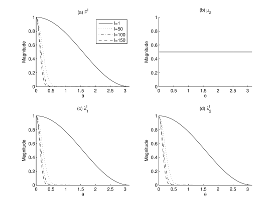
Figure 2: Frequency responses of a (Gaussian) matrix of filters with $b=1$, $c=1$, and $d=0$.

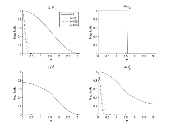
Figure 3: Frequency responses of a (Gaussian) matrix of filters with $b=1$, $c=1/2$, and $d=0$.

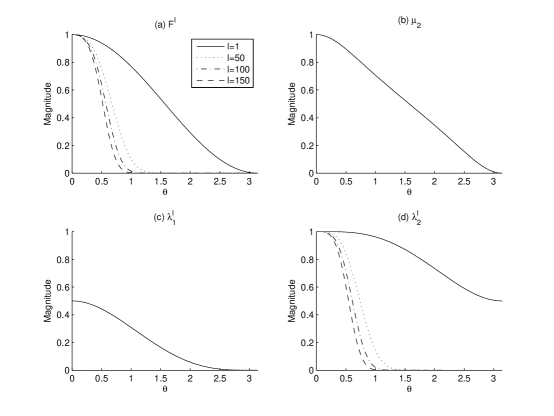
Figure 4: Frequency responses of a matrix of filters with $b=1$, $c=0$, and $d=-0.5$.

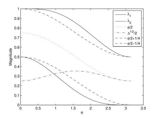
Figure 5: Close-up of eigenfunctions and their constituents with $b=1$, $c=0$, and $d=-0.5$.

Figure 6: Comparison of two filters: Gaussian ($b=1$, $c=d=0$) and Non-Gaussian ($b=1$, $c=0$, $d=-0.5$).

Another design philosophy to consider is to create a sharp cut-off in the frequency response profile. Under such approach, we may want to find a set of parameters that maximizes $F^{l}(\pi/16)-F^{l}(\pi/4)$ at say $l=100$, while satisfying the constraints of Theorem 4.2. This is a non-convex optimization problem and can be solved numerically with various software packages.

By a Matlab$\circledR$ Optimization toolbox, we obtained $b=1$, $c=0.48$, and $d=-0.26$. The result was not sensitive to initial conditions, which were set randomly. The frequency response of the filter at $l=100$ is shown in Figure 7 along with the response of the Gaussian counterpart. The amount of fall-off for the non-Gaussian case is 0.93 while that of the Gaussian case is 0.41 and that of a non-Gaussian case with $b=1$, $c=0$ and $d=-0.5$ (the filter shown in Figure 4) is 0.83.

Figure 7: Comparison of two filters at $l=100$: Gaussian ($b=1$, $c=d=0$) and Non-Gaussian ($b=1$, $c=0.48$, $d=-0.26$). The parameters for the non-Gaussian case are obtained by constrained non-linear optimization to maximize the fall off between $\theta=\pi/16$ and $\theta=\pi/4$ (in other words, $F^{l}(\pi/16)-F^{l}(\pi/4)$.). The fall-off for the Gaussian case is 0.93, and that for the Gaussian case is 0.41.

6 Discussion

One question that naturally arise from the illustration given in Figure 5 regarding the frequency profiles of the constituents is if it is possible to generate the same frequency response of the matrix of filters by using a conventional convolution kernel with a larger support (more than 3 non-zero coefficients). For example, we can use an equivalent filter at some $l$ as the convolution kernel. The answer to the question is no, since the formulae of the frequency responses for the two cases are different; For a conventional convolution based case,

$$F^{l}(\theta)=\left(K(\theta)\right)^{l},$$ (105)

where $K$ is the frequency response of the convolution kernel. On the other hand, the frequency response of a matrix of filters is given by

$$F^{l}(\theta)=\mu_{1}(\theta)\left(\lambda_{1}(\theta)\right)^{l}+\mu_{2}(\theta)\left(\lambda_{2}(\theta)\right)^{l}.$$ (106)

Thus, (105) cannot generate (106) in general. As seen in Section 5, the converse is not true, and (106) can generate any instance of (105) by setting $\sigma_{xx}(\theta)=K(\theta)$ and $d=0$.

In this paper, we have limited our study to the $2\times 2$ case. Even with such minimal configuration, the resulting equivalent filter is able to construct a non-trivial (or non-Gaussian) scale space. With larger configuration, we expect that more elaborate frequency responses are possible. Note that the original EQW employed a $3\times 3$ matrix of filters. It is however, difficult to extend the analysis described in this paper to the general case. Closed form expressions of eigenvalues are not possible for $P>4$, and although they exist for $P\leq 4$, deriving sufficient conditions for scale space filtering can be extremely complicated.

We can extend the matrix size while imposing some structural constraints on the matrix. For example, we can consider a $P\times P$ matrix of filters that are circulant. Then, we will be able to derive a simple expression for the frequency response of the equivalent filters. In this case, the mixing coefficients are all $1/P$, thus the frequency response of the equivalent filter becomes

$$F^{l}(\theta)=\frac{1}{P}\sum_{j=0}^{P}\lambda_{j}^{l}(\theta)$$ (107)

with

$$\lambda_{j}(\theta)=\sum_{k=0}^{P}F_{1k}(\theta)\rho_{P}^{jk}$$ (108)

where $F_{1k}$ is the frequency response of $\mathbf{f}_{1k}$ and $\rho_{P}$ is the $P$th root of unity. Note that at $P=2$, this circulant configuration leads to $\sigma_{xx}=\sigma_{aa}$ and in turn leads a Gaussian scale space. It is not clear if the same can be said for $P>2$.

Without closed form expressions of eigenvalues, we resort to numerical schemes. Give a matrix of filter, we want to test if the filter satisfies the scale space requirements. We need to come up with numerical conditions that guarantee the positivity and unimodality requirements at every $\theta$ and the constant reduction requirement at every $l$.

So far, we assumed that each convolution filter is circulant. We can extend the results for non-circulant filter with some type of extension schemes such as zero padding and reflection, given an upper limit of the iteration number. Let $L$ be the upper limit of the iteration number. Then, the length of the equivalent filter is at most $2L+1$. Then the result of the iterative filtering can be obtained by first extending the original signal by $L$ on both ends by the chosen extension scheme, apply the circulant filters to the extended signal, and truncate the result at the portion of the original signal. Thus, non-circulant filter can be implemented by circulant one with proper extension. Given a scale space of a signal (i.e. a collection of signals that satisfy the scale space requirements), a truncated portion of the signal also satisfies the scale space requirements. Thus, the sufficient condition for the scale space filter remains applicable to the non-circulant case.

7 Conclusion

In this paper, we first derived the frequency response of a general matrix of filters applied iteratively to the signal. The response is a convex combination of the power of eigen-functions describing the impulse response of the filter. We then studied a $2\times 2$ matrix of filters and derive sufficient conditions for it to be a scale space kernel. We showed that the $2\times 2$ matrix of filters can generate non-Gaussian scale space, thus are more powerful than the conventional convolution kernel.

Future research goals include extension of the study to more general matrix sizes. We suggest investigating some general cases such as circulant one and tri-diagonal one, and derive sufficient conditions for the scale space requirements. For more general cases, we suggest deriving a numerical test that checks if the given configuration satisfies the scale space requirements.

References

- [1] T. Kubota, “A shape representation with elastic quadratic polynomials–preservation of high curvature points under noisy conditions,” International Journal Computer Vision, vol. 82, no. 2, pp. 133–155, 2009.
- [2] A. Witkin, “Scale-space filtering,” in Proc. 8th Int’l Joint Conf. Artificial Intelligence, 1983, pp. 1019–1022.
- [3] T. Lindeberg, “Scale-space for discrete signals,” IEEE Trans. Pattern Analysis and Machine Intelligence, vol. 12, no. 3, pp. 234–254, March 1990.
- [4] J. J. Koenderink, “The structure of images,” Biological Cybernetics, vol. 50, pp. 363–370, 1984.
- [5] J. Babaud, A. P. Witkin, M. Baudin, and R. O. Duda, “Uniqueness of the gaussian kernel for scale space filtering,” IEEE Trans. Pattern Analysis and Machine Intelligence, vol. 8, no. 1, pp. 26–33, January 1986.
- [6] A. L. Yuiile and T. A. Poggio, “Scaling theorem for zero crossings,” IEEE Trans. Pattern Analysis and Machine Intelligence, vol. 8, no. 1, pp. 15–25, January 1986.