Measurement of the $CP$-violating phase $\phi_{s}^{J/\psi\phi}$ at DØ

Abstract

This paper is a report of an updated measurement of the $CP$-violating phase $\phi_{s}^{J/\psi\phi}$ and the decay width difference for the two mass eigenstates $\Delta\Gamma_{s}$ from flavor-tagged decay ${B_{s}^{0}\rightarrow J/\psi\phi}$. The 68% confidence level intervals, including systematic uncertainties, are $\phi_{s}^{J/\psi\phi}=-0.55^{+0.38}_{-0.36}$ and $\Delta\Gamma_{s}=0.163^{+0.065}_{-0.064}$ ps^-1. This measurement is in agreement with SM expected value, the $p$-value for the Standard Model point is 29.8%. The data sample corresponds to an integrated luminosity of 8.0 fb^-1 accumulated with the D0 detector using $p\overline{p}$ collisions at $\sqrt{s}=1.96$ TeV produced at the Fermilab Tevatron collider.

I Introduction

In the standard model (SM), the light ($L$) and heavy ($H$) mass eigenstates of the mixed $B_{s}^{0}$ system are expected to have sizeable mass and decay width differences: $\Delta M_{s}\equiv M_{H}-M_{L}$ and $\Delta\Gamma_{s}\equiv\Gamma_{L}-\Gamma_{H}$. The two mass eigenstates are expected to be almost pure $CP$ eigenstates. The $CP$-violating phase that appears in $b\rightarrow c\overline{c}s$ decays, due to the interference of the decay with and without mixing, is predicted LN2006 to be $\phi_{s}^{J/\psi\phi}=-2\beta_{s}=2\arg[-V_{tb}V^{*}_{ts}/V_{cb}V^{*}_{cs}]=-0.038\pm 0.002$, where $V_{ij}$ are elements of the Cabibbo-Kobayashi-Maskawa quark-mixing matrix ckm . New phenomena may alter the observed phase UTfit to $\phi_{s}^{J/\psi\phi}\equiv-2\beta_{s}+\phi_{s}^{\Delta}$.

The first direct constraint on $\phi_{s}^{J/\psi\phi}$  prl07 was derived by analyzing ${B_{s}^{0}\rightarrow J/\psi\phi}$ decays where the flavor (i.e., $B^{0}_{s}$ or $\overline{B}^{0}_{s}$) at the time of production was not determined (“tagged”). It was followed by an improved analysis prl08 , based on 2.8 fb^-1 of integrated luminosity, that included the information on the $B_{s}^{0}$ flavor at production. In that analysis we measured $\Delta\Gamma_{s}$ and the average lifetime of the ${B_{s}^{0}}$ system, $\overline{\tau}_{s}=1/\overline{\Gamma}_{s}$, where $\overline{\Gamma}_{s}\equiv(\Gamma_{H}+\Gamma_{L})/2$. The $CP$-violating phase $\phi_{s}^{J/\psi\phi}$ was also extracted for the first time. The measurement correlated two solutions for $\phi_{s}^{J/\psi\phi}$ with two corresponding solutions for $\Delta\Gamma_{s}$. Improved precision was obtained by refitting the results using additional experimental constraints combo . Here we present new results from the time-dependent amplitude analysis of the decay ${B_{s}^{0}\rightarrow J/\psi\phi}$  using a data sample corresponding to an integrated luminosity of 8.0 fb^-1 collected with the D0 detector run2det at the Fermilab Tevatron Collider. We measure $\Delta\Gamma_{s}$; the average lifetime of the ${B_{s}^{0}}$ system, $\overline{\tau}_{s}=1/\overline{\Gamma}_{s}$, where $\overline{\Gamma}_{s}\equiv(\Gamma_{H}+\Gamma_{L})/2$; and the CP-violating phase $\phi_{s}^{J/\psi\phi}$.

II Data Sample and Event Reconstruction

The analysis presented here is based on data accumulated between February 2002 and June 2010, corresponds to 8 fb^-1 of integrated luminosity.

We reconstruct the decay chain ${B_{s}^{0}\rightarrow J/\psi\phi}$, $J/\psi\rightarrow\mu^{+}\mu^{-}$, $\phi\rightarrow K^{+}K^{-}$ from candidate ($J/\psi,\phi$) pairs consistent with coming from a common vertex and having an invariant mass in the range $5.37\pm 0.20$ GeV. Events are collected with a mixture of single and dimuon triggers. To avoid a bias in the $B_{s}^{0}$ lifetime distribution events are rejected if they only satisfy triggers that impose a requirement on the track impact parameter with respect to the $p\overline{p}$ interaction vertex.

$B^{0}_{s}$ candidate events are required to include two opposite-sign muons accompanied by two opposite-sign tracks. Both muons are required to be detected in the muon chambers inside the toroid magnet and at least one of the muons is required to be also detected outside the toroid. Invariant mass range for muon pairs is $3.096\pm 0.350$ GeV, consistent with $J/\psi$ decay. $J/\psi$ candidates are combined with pairs of oppositely charged tracks (assigned the kaon mass) consistent with production at a common vertex, and with an invariant mass in the range $1.019\pm 0.030$ GeV. Each of the four final-state tracks is required to have at least one SMT hit.

A kinematic fit under the $B_{s}^{0}$ decay hypothesis constrains the dimuon invariant mass to the world-average $J/\psi$ mass PDG and constrains the four-track system to a common vertex. In events where multiple candidates satisfy these requirements, we select the candidate with the best decay vertex fit probability.

The primary vertex (PV) is reconstructed using tracks that do not originate from the candidate $B_{s}^{0}$ decay, and apply a constraint to the average beam-spot position in the transverse plane. We define the signed decay length of a ${B_{s}^{0}}$ meson, $L^{B}_{xy}$, as the vector pointing from the PV to the decay vertex, projected on the ${B_{s}^{0}}$ transverse momentum $p_{T}$. The proper decay time of a ${B_{s}^{0}}$ candidate is given by $t=M_{B_{s}}\vec{L}_{xy}^{B}\cdot\vec{p}/(p_{T}^{2})$ where $M_{B_{s}}$ is the world-average ${B_{s}^{0}}$ mass PDG , and $\vec{p}$ is the particle momentum. The distance in the beam direction between the PV and the $B_{s}^{0}$ vertex is required to be less than 5 cm. Approximately 5 million events are accepted after the selection described in this section.

III Background Suppression

The selection criteria are designed to optimize the measurement of $\phi_{s}^{J/\psi\phi}$ and $\Delta\Gamma_{s}$. Most of the background is due to directly produced $J/\psi$ mesons accompanied by tracks arising from hadronization. This “prompt” background is distinguished from the “non-prompt”, or “inclusive $B\rightarrow J/\psi+X$” background, where the $J/\psi$ meson is a product of a $b$-hadron decay while the tracks forming the $\phi$ candidate emanate from a multi-body decay of a $b$ hadron or from hadronization. Two different event selection approaches are used, one based on a multi-variate technique, and one based on simple limits on kinematic and event quality parameters.

Three Monte Carlo (MC) samples are used to study background suppression: signal, prompt background, and non-prompt background. All three are generated with pythia pythia . Hadronization is also done in pythia, but all hadrons carrying heavy flavors are passed on to EvtGen evtgen to model their decays. The prompt background MC sample consists of $J/\psi\to\mu^{+}\mu^{-}$ decays produced in $gg\to J/\psi g$, $gg\to J/\psi\gamma$, and $g\gamma\to J/\psi g$ processes. The signal and non-prompt background samples are generated from primary $b\bar{b}$ pair production with all $b$ hadrons being produced inclusively and the $J/\psi$ mesons forced into $\mu^{+}\mu^{-}$ decays. For the signal sample, events with a ${B_{s}^{0}}$  are selected, their decays to $J/\psi\phi$ are implemented without mixing and with uniform angular distributions, and the ${B_{s}^{0}}$ mean lifetime is set to $\overline{\tau}_{s}$ = 1.464 ps. There are approximately 10⁶ events in each background and the signal MC samples. All events are passed through a full standard chain of geant-based Geant detector software of DØ simulation.

IV Multivariate event selection

To discriminate the signal from background events, we use the TMVA package refroot . In preliminary studies using MC simulation, the Boosted Decision Tree (BDT) algorithm was found to demonstrate the best performance. Since prompt and non-prompt backgrounds have different kinematic behavior, we train two discriminants, one for each type of background. We use a set of 33 variables for the prompt background and 35 variables for the non-prompt background.

To choose the best set of criteria for the two BDT discriminants, we start with 14 data samples with signal yeilds ranging from 4000 to 7000 events. For each sample we choose the pair of BDT cuts which gives the highest significance S/sqrt(S+B), where $S$ ($B$) is the number of signal (background) events in the data sample. Figure 1(a) shows the number of signal events as a function of the total number of events for the 14 points. As the BDT criteria are loosened, the total number of events increases by a factor of ten, while the number of signal events increases by about 50%.

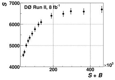
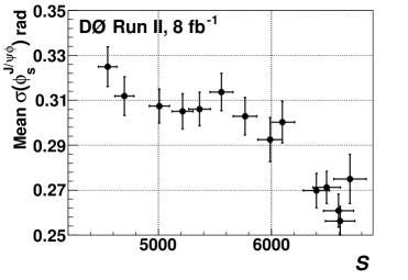
Figure 1: (a) Number of ${B_{s}^{0}\rightarrow J/\psi\phi}$ signal events as a function of the total number of events for the 14 criteria sets considered.     (b) Mean value of $\sigma(\phi_{s})$ as a function of the number of signal events.

The choice of the final cut on the BDT output is based on an ensemble study. We perform a maximum-likelihood fit to the event distribution in the 2-dimensional (2D) space of $B_{s}^{0}$ candidate mass and proper time. This 2D fit provides a parametrization of the background mass and proper time distribution. We then generate pseudo-experiments in the 5D space of $B_{s}^{0}$ candidate mass, proper time, and three independent angles of decay products, using as input the parameters as obtained in a preliminary study, and the background from the 2D fit. We perform a 5D maximum likelihood fit on the ensembles and compare the distributions of the statistical uncertainties of $\phi_{s}^{J/\psi\phi}$ ($\sigma(\phi_{s}^{J/\psi\phi})$) and $\Delta\Gamma_{s}$ ($\sigma(\Delta\Gamma_{s})$) for the different sets of criteria. The dependence of the mean values of $\sigma(\phi_{s}^{J/\psi\phi})$ on the number of signal events is shown in Figure 1(b).

The mean statistical uncertainties of both $\phi_{s}^{J/\psi\phi}$ and $\Delta\Gamma_{s}$ systematically decrease with increasing signal, favoring looser cuts. The gain in the parameter resolution is slower for the three loosest criteria, while the total number of events doubles from about 0.25$\times 10^{6}$ to 0.5$\times 10^{6}$. The fits used for these ensemble tests were simplified, therefore the magnitude of the predicted uncertainty is expected to underestimate the final measured precision. However, the general trends should be valid. Based on these results, we choose the sample that contains about 6500 signal events.

We select a second event sample by applying criteria on event quality and kinematic quantities. We use the consistency of the results obtained for the BDT and for this sample as a measure of systematic effects related to imperfect modeling of the detector acceptance and of the selection requirements. The criteria are the same as in Refs. prl07 and prl08 . We refer to this second sample as the “Square-cuts” sample.

V Flavor Tagging

At the Tevatron, $b$ quarks are mostly produced in $b\overline{b}$ pairs. The flavor of the initial state of the $B_{s}^{0}$ candidate is determined by exploiting properties of particles produced by the other $b$ hadron (“opposite-side tagging”, or OST). The OST-discriminating variables are based primarily on the presence of a muon or an electron from the semi-leptonic decay of the other $b$ hadron produced in the $p\overline{p}$ interaction. If a charged lepton is not found, the algorithm attempts to reconstruct the decay vertex of the opposite-side $b$ hadron and determine the net charge of particles forming the vertex.

The OST algorithm, based on the Likelihood Ratio method, assigns to each event a value of the predicted tagging parameter $d$, in the range [$-1$,1], with $d>0$ tagged as an initial $b$ quark and $d<0$ tagged as an initial $\overline{b}$ quark. Larger $|d|$ values correspond to higher tagging confidence. In events where no tagging information is available $d$ is set to zero. The efficiency $\epsilon$ of the OST, defined as fraction of the number of candidates with $d\neq 0$, is 18%. The OST-discriminating variables and algorithm are described in detail in Ref. bflavor .

The tagging dilution ${\cal D}$ is defined as $\cal{D}=N_{\rm cor}-N_{\rm wr}/(N_{\rm cor}+N_{\rm wr})$    where $N_{\rm cor}$ ($N_{\rm wr}$) is the number of events with correctly (wrongly) identified initial $B$-meson flavor.

The dependence of the tagging dilution on the tagging parameter $d$ is calibrated with data for which the flavor ($B$ or $\overline{B}$) is known. The dilution calibration is based on four independent $B_{d}^{0}\to\mu\nu D^{*\pm}$ data samples corresponding to different time periods. For each sample we perform an analysis of the $B_{d}^{0}-\overline{B}_{d}^{0}$ oscillations described in Ref. Abazov:2006dm . We divide the samples in five ranges of the tagging parameter $|d|$, and for each range we obtain a mean value of the dilution ${\cal|D|}$. The mixing frequency $\Delta M_{d}$ is fitted simultaneously and is found to be stable and consistent with the world average value. The measured values of the tagging dilution $\cal|D|$ for the running period of time is parametrized by function:

$${\cal|D|}=\frac{p_{0}}{(1+\exp((p_{1}-|d|)/p_{2}))}-\frac{p_{0}}{(1+\exp(p_{1}/p_{2}))}.$$ (1)

and the function is fitted to the data. There is a good agreement in the fits for running period of time, and hence a weighted average is taken.

VI Maximum Likelihood Fit

We perform a six-dimensional (6D) unbinned maximum likelihood fit to the proper decay time and its uncertainty, three decay angles characterizing the final state, and the mass of the $B_{s}^{0}$ candidate. We use events for which the invariant mass of the $K^{+}K^{-}$ pair is within the range 1.01 – 1.03 GeV. There are 104683 events in the BDT-based sample and 66455 events in the Square-cuts sample. We adopt the formulae and notation of Ref. formulae . The normalized functional form of the differential decay rate includes an $\cal S$-wave $KK$ contribution in addition to the dominant $\cal P$-wave $\phi\rightarrow K^{+}K^{-}$ decay. To model the distributions of the signal and background we use the software library RooFit refroofit .

VI.1 Signal model

The angular distribution of the signal is expressed in the transversity basis. In the coordinate system of the $J/\psi$ rest frame, where the $\phi$ meson moves in the $x$ direction, the $z$ axis is perpendicular to the decay plane of $\phi\to K^{+}K^{-}$, and $p_{y}(K^{+})\geq 0$. The transversity polar and azimuthal angles $\theta$ and $\varphi$ describe the direction of the positively-charged muon, while $\psi$ is the angle between $\vec{p}(K^{+})$ and $-\vec{p}(J/\psi)$ in the $\phi$ rest frame.

In the transversity basis, the decay amplitude of the $B_{s}^{0}$ and $\overline{B}_{s}^{0}$ mesons is decomposed into three independent components corresponding to linear polarization states of the vector mesons $J/\psi$ and $\phi$, which are polarized either longitudinally (0) or transversely to their direction of motion, and parallel ($\parallel$) or perpendicular ($\perp$) to each other.

The time dependence of amplitudes ${\cal A}_{i}(t)$ and ${\bar{\cal A}_{i}}(t)$ ($i$ denotes one of $\{||,\perp,0\}$), for $B_{s}^{0}$ and $\overline{B}_{s}^{0}$ states to reach the final state $J/\psi$ $\phi$ is:

$${\cal A}_{i}(t) = F(t)\left[E_{+}(t)\pm e^{2i\beta_{s}}E_{-}(t)\right]a_{i}\,,$$

$${\bar{\cal A}_{i}}(t) = F(t)\left[\pm E_{+}(t)+e^{-2i\beta_{s}}E_{-}(t)\right]a_{i}\,$$ (2)

where

$$F(t) = \frac{e^{-\Gamma_{s}t/2}}{\sqrt{\tau_{H}+\tau_{L}\pm\cos{2\beta_{s}}\left(\tau_{L}-\tau_{H}\right)}}\,,$$ (3)

and $\tau_{H}$ and $\tau_{L}$ are the lifetimes of the heavy and light $B_{s}^{0}$ eigenstates.

In the above equations the upper sign indicates a CP-even final state, the lower sign indicates a CP-odd final state,

$$E_{\pm}(t)\equiv\frac{1}{2}\left[e^{\left(\frac{-\Delta\Gamma_{s}}{4}+i\frac{\Delta M_{s}}{2}\right)t}\pm e^{-\left(\frac{-\Delta\Gamma_{s}}{4}+i\frac{\Delta M_{s}}{2}\right)t}\right],$$ (4)

and the amplitude parameters $a_{i}$ give the time-integrated decay rate to each of the polarization states, $|a_{i}|^{2}$, satisfying:      $\sum_{i}{|a_{i}|^{2}}$ = 1.    The normalized probability density functions $P_{B_{z}}$ ($X_{z}$ denotes one more same equation replaced by $\bar{X_{z}}$)

$$P_{B_{z}}(\theta,\varphi,\psi,t)=\frac{9}{16\pi}|{\bf A_{z}}(t)\times\hat{n}|^{2},$$

(5)

where $\hat{n}$ is the muon momentum direction in the $J/\psi$ rest frame,

$$\hat{n}=\left(\sin{\theta}\cos{\varphi},\sin{\theta}\sin{\varphi},\cos{\theta}\right),$$ (6)

and ${\bf A}(t)$ and ${\bf{\bar{A}}}(t)$ are complex vector functions of time defined as

$${\bf A_{z}}(t)=\left({\mathcal{(}A_{z})}_{0}(t)\cos{\psi},-\frac{{\mathcal{(}A_{z})}_{\parallel}(t)\sin{\psi}}{\sqrt{2}},i\frac{{\mathcal{(}A_{z})}_{\perp}(t)\sin{\psi}}{\sqrt{2}}\right),$$

(7)

The values of ${\cal A}_{i}(t)$ at $t=0$ are denoted as $A_{i}$. They are related to the parameters $a$ by

$$|A_{i}|^{2}=\frac{|a_{i}|^{2}y}{1+(y-1)|a_{\perp}|^{2}},$$

where $y\equiv(1-z)/(1+z)$ and $z\equiv\cos{2\beta_{s}}\Delta\Gamma_{s}/(2\overline{\Gamma}_{s})$. By convention, the phase of $A_{0}$ is set to zero and the phases of the other two amplitudes are denoted by $\delta_{||}$ and $\delta_{\perp}$.

For a given event, the decay rate is the sum of the functions $P_{B}$ and $P_{\bar{B}}$ weighted by the flavor tagging dilution factors $(1+{\cal D})/2$ and $(1-{\cal D})/2$, respectively.

The contribution from the decay to $J/\psi K^{+}K^{-}$ with the kaons in an $\cal S$ wave is expressed in terms of the $\cal S$-wave fraction $F_{S}$ and a phase $\delta_{s}$. The squared sum of the $\cal P$ and $\cal S$ waves is integrated over the $KK$ mass. For the $\cal P$ wave, we assume the non-relativistic Breit-Wigner model

$$g(M(KK))=\sqrt{\frac{\Gamma_{\phi}/2}{\Delta M(KK)}}\cdot\frac{1}{M(KK)-M_{\phi}+i\Gamma_{\phi}/2}$$ (9)

with the $\phi$ meson mass $M_{\phi}=1.019$ GeV and width $\Gamma_{\phi}=4.26$ MeV PDG , and with $\Delta M(KK)=0.02$ GeV.

For the $\cal S$-wave component, we assume a uniform distribution in the range $1.01<M(KK)<1.03$ GeV. In the case of the BDT selection, it is modified by a $KK$-mass dependent factor corresponding to the BDT selection efficiency. We constrain the oscillation frequency to $\Delta M_{s}=17.77\pm 0.12$ ps^-1, as measured in Ref. dms . Table 1 lists all physics parameters used in the fit.

Parameter	Definition
$|A_{0}|^{2}$	$\cal P$-wave longitudinal amplitude squared, at $t=0$
$A1$	$|A_{\|}|^{2}/(1-|A_{0}|^{2})$
$\overline{\tau}_{s}$ (ps)	$B^{0}_{s}$ mean lifetime
$\Delta\Gamma_{s}$ (ps-1)	Heavy-light decay width difference
$F_{S}$	$K^{+}K^{-}$ $\cal S$-wave fraction
$\beta_{s}$	CP-violating phase ( $\equiv-\phi_{s}^{J/\psi\phi}/2$)
$\delta_{\|}$	$\arg(A_{\|}/A_{0})$
$\delta_{\perp}$	$\arg(A_{\perp}/A_{0})$
$\delta_{s}$	$\arg(A_{s}/A_{0})$

Table 1: Definition of nine real measurables for the decay ${B_{s}^{0}\rightarrow J/\psi\phi}$ used in the Maximum Likelihood fitting.

For the signal mass distribution we use a Gaussian function with a free mean value, width, and normalization. The function describing the signal rate in the 6D space is invariant under the combined transformation $\beta_{s}\rightarrow\pi/2-\beta_{s}$, $\Delta\Gamma_{s}\rightarrow-\Delta\Gamma_{s}$, $\delta_{\|}\rightarrow 2\pi-\delta_{\|}$, $\delta_{\perp}\rightarrow\pi-\delta_{\perp}$, and $\delta_{s}\rightarrow\pi-\delta_{s}$. In addition, with a limited flavor-tagging power, there is an approximate symmetry around $\beta_{s}=0$ for a given sign of $\Delta\Gamma_{s}$.

We correct the signal decay rate by a detector acceptance factor $\epsilon(\psi,\theta,\varphi)$ parametrized by coefficients of expansion in Legendre polynomials $P_{k}(\psi)$ and real harmonics $Y_{lm}(\theta,\varphi)$. The coefficients are obtained from Monte Carlo simulation.

VI.2 Background model

The proper decay time distribution of the background is described by a sum of a prompt component, modeled as a Gaussian function centered at zero, and a non-prompt component. The non-prompt component is modeled as a superposition of one exponential decay for $t<0$ and two exponential decays for $t>0$, with free slopes and normalizations. The lifetime resolution is modeled by an exponential convoluted with a Gaussian function, with two separate parameters for prompt and non-prompt background. To allow for the possibility of the lifetime uncertainty to be systematically underestimated, we introduce a free scale factor.

The mass distributions of the two components of background are parametrized by low-order polynomials: a linear function for the prompt background and a quadratic function for the non-prompt background. The angular distribution of background is parametrized by Legendre and real harmonics expansion coefficients. A separate set of expansion coefficients $c^{k}_{lm}$ and $c^{k}_{lm}$, with $k=0$ or $2$ and $l=0,1,2$, is used for the prompt and non-prompt background. A preliminary fit is first performed with all $17\times 2$ parameters allowed to vary. In subsequent fits those that converge at values within two standard deviations of zero are set to zero. Nine free parameters remain, five for non-prompt background: $c^{0}_{1-1}$, $c^{0}_{20}$, $c^{0}_{22}$, $c^{2}_{00}$, and $c^{2}_{22}$, and four for prompt background: $c^{0}_{1-1}$, $c^{0}_{20}$, $c^{0}_{22}$, and $c^{2}_{2-1}$. All background parameters described above are varied simultaneously with physics parameters. In total, there are 36 parameters used in the fit. In addition to the nine physics parameters defined in Table 1, they are: signal yield, mean mass and width, non-prompt background contribution, six non-prompt background lifetime parameters, four background time resolution parameters, one time resolution scale factor, three background mass distribution parameters, and nine parameters describing background angular distributions.

VI.3 Systematic uncertainties

There are several possible sources of systematic uncertainty in the measurements. These uncertainties are estimated for:

• Flavor tagging: The nominal calibration of the flavor tagging dilution is determined as a weighted average of four samples separated by the running period. As an alternative, we use two separate calibration parameters, for the same running period. We also alter the nominal parameters by their uncertainties.

• Proper decay time resolution: Fit results can be affected by the uncertainty of the assumed proper decay time resolution function. To assess the effect, we have used two alternative parameterizations obtained by random sampling of the resolution function.

• Detector acceptance: The effects of imperfect modeling of the detector acceptance and of the selection requirements are estimated by investigating the consistency of the fit results for the sample based on the BDT selection and on the Square-cuts selection. Although the overlap between the two samples is 70%, and some statistical differences are expected, we interpret the differences in the results as a measure of systematic effects.

• $M(KK)$ resolution: The limited $M(KK)$ resolution may affect the results of the analysis, especially the phases and the $\cal S$-wave fraction $F_{S}$, through the dependence of the $\cal S-\cal P$ interference term on the $\cal P$-wave mass model. We repeat the fits using this altered $\phi(1020)$ propagator as a measure of the sensitivity to the $M(KK)$ resolution.

The differences between the best-fit values and the alternative fit values provide a measure of systematic effects. For the best estimate of the C.L. ranges for all the measured physics quantities, we conduct Markov Chain Monte Carlo (MCMC) technique described in the next section.

VII Confidence intervals from MCMC studies

The maximum likelihood fit provides the best values of all free parameters, including the signal observables and background model parameters, their statistical uncertainties and their full correlation matrix.

In addition to the free parameters determined in the fit, the model depends on a number of external constants whose inherent uncertainties are not taken into account in a given fit. Ideally, effects of uncertainties of external constants, such as time resolution parameters, flavor tagging dilution calibration, or detector acceptance, should be included in the model by introducing the appropriate parametrized probability density functions and allowing the parameters to vary. Such a procedure of proper integrating over the external parameter space would greatly increase the number of free parameters and would be prohibitive. Therefore, as a trade-off, we apply a random sampling of external parameter values within their uncertainties, we perform the analysis for thus created “alternative universes”, and we average the results. To do the averaging in the multidimensional space, taking into account non-Gaussian parameter distributions and correlations, we use the MCMC technique.

The MCMC technique uses the Metropolis-Hastings algorithm MetHast to generate a random sample proportional to a given probability distribution. The algorithm generates a sequence of “states”, a Markov chain, in which each state depends only on the previous state.

To generate a Markov chain for a given maximum likelihood fit result, we start from the best-fit point $x$. We randomly generate a point $x^{\prime}$ according to the multivariate normal distribution $\exp(-(x^{\prime}-x)\cdot\Sigma\cdot(x^{\prime}-x)/2)$, where $\Sigma$ is the covariance matrix. The new point is accepted if ${\cal L}(x^{\prime})/{\cal L}(x)>1$, otherwise it is accepted with the probability ${\cal L}(x^{\prime})/{\cal L}(x)$. The process is continued until a desired number of states is achieved. To avoid a bias due to the choice of the initial state, we discard the early states which may “remember” the initial state. Our studies show that the initial state is “forgotten” after approximately 50 steps. We discard the first 100 states in each chain.

While we do not use any external numerical constraints on the polarization amplitudes, we note that the best-fit values of their magnitudes and phases are consistent with those measured in the $U(3)$-flavor related decay ${B_{d}^{0}\rightarrow J/\psi K^{*}}$ PDG , up to the sign ambiguities. Ref. gr predicts that the phases of the polarization amplitudes in the two decay processes should agree within approximately 0.17 radians. For $\delta_{\perp}$, our measurement gives equivalent solutions near $\pi$ and near zero, with only the former being in agreement with the value of $2.91\pm 0.06$ measured for ${B_{d}^{0}\rightarrow J/\psi K^{*}}$ by $B$ factories. Therefore, in the following we limit the range of $\delta_{\perp}$ to $\cos\delta_{\perp}<0$.

VII.1 Results

The fit assigns $5598\pm 113$ ($5050\pm 105$) events to the signal for the BDT (Square-cuts) sample. A single fit does not provide meaningful point estimates and uncertainties for the four phase parameters. Their estimates are obtained using the MCMC technique.

Figure 2 shows 68%, 90% and 95% C.L. contours in the ($\phi_{s}^{J/\psi\phi}$,$\Delta\Gamma_{s}$) plane for the BDT-based and for the Square-cuts samples. The point estimates of physics parameters are obtained from one-dimensional projections. The minimal range containing 68% of the area of the probability density function defines the one standard deviation C.L. interval for each parameter, while the most probable value defines the central value.

The one-dimensional estimates of physics parameters for the BDT-cuts and Square-cuts sample are shown in Table 2.

Parameter	BDT-cut sample	Square-Cut sample	Final Result
$\overline{\tau}_{s}$ (ps)	$1.426^{+0.035}_{-0.032}$	$1.444^{+0.041}_{-0.033}$	$1.443^{+0.038}_{-0.035}$
$\Delta\Gamma_{s}$ (ps-1)	$0.129^{+0.076}_{-0.053}$	$0.179^{+0.059}_{-0.060}$	$0.163^{+0.065}_{-0.064}$
$\phi_{s}^{J/\psi\phi}$	$-0.49^{+0.48}_{-0.40}$	$-0.56^{+0.36}_{-0.32}$	$-0.55^{+0.38}_{-0.36}$
$|A_{0}|^{2}$	$0.552^{+0.016}_{-0.017}$	$0.565\pm 0.017$	$0.558^{+0.017}_{-0.019}$
$|A_{\parallel}|^{2}$	$0.219^{+0.020}_{-0.021}$	$0.249^{+0.021}_{-0.022}$	$0.231^{+0.024}_{-0.030}$
$\delta_{\|}$	$3.15\pm 0.27$	$3.15\pm 0.19$	$3.15\pm 0.22$
$\cos(\delta_{\perp}-\delta_{s})$	$-0.06\pm 0.24$	$-0.20^{+0.26}_{-0.27}$	$-0.11^{+0.27}_{-0.25}$
$F_{S}$	$0.146\pm 0.035$	$0.173\pm 0.036$	$0.173\pm 0.036$

Table 2: The one-dimensional estimates of physics parameters for the BDT-cuts sample, Square-cuts sample and final result values with systematic error.

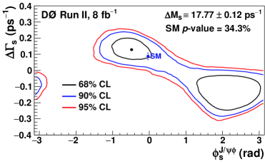
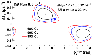
Figure 2: Two-dimensional 68%, 90% and 95% C.L. contour for BDT and Square cuts selection. The standard model expectation is indicated as a point with an error.

To obtain the final C.L. ranges for physics parameters, we combine all eight MCMC chains, effectively averaging the probability density functions of the results of the fits to the BDT- and Square-cuts samples. Figure 3 shows 68%, 90% and 95% C.L. contours in the ($\phi_{s}^{J/\psi\phi}$,$\Delta\Gamma_{s}$) plane. The $p$-value for the SM point ln2011 ($\phi_{s}^{J/\psi\phi},\Delta\Gamma_{s})=(-0.038,0.087$ ps^-1) is 29.8%.

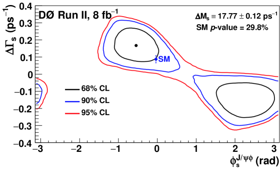
Figure 3: Two-dimensional 68%, 90% and 95% C.L. contours including systematic uncertainties. The standard model expectation is indicated as a point with an error.

VIII Summary and Discussion

We have presented a time-dependent angular analysis of the decay process ${B_{s}^{0}\rightarrow J/\psi\phi}$. We measure $B_{s}^{0}$ mixing parameters, average lifetime, and decay amplitudes. In addition, we measure the amplitudes and phases of the polarization amplitudes. We also measure the level of the $KK$ $\cal S$-wave contamination in the mass range $1.01$ – $1.03$ GeV, $F_{S}$. The final result values for the 68% C.L. intervals, including systematic uncertainties, with the oscillation frequency constrained to $\Delta M_{s}=17.77\pm 0.12$ ps^-1, are shown in the last column of Table 2. The $p$-value for the SM point ($\phi_{s}^{J/\psi\phi},\Delta\Gamma_{s})=(-0.038,0.087$ ps^-1) is 29.8%.

We thank the staffs at Fermilab and collaborating institutions, and acknowledge support from the DOE and NSF (USA); CEA and CNRS/IN2P3 (France); FASI, Rosatom and RFBR (Russia); CNPq, FAPERJ, FAPESP and FUNDUNESP (Brazil); DAE and DST (India); Colciencias (Colombia); CONACyT (Mexico); KRF and KOSEF (Korea); CONICET and UBACyT (Argentina); FOM (The Netherlands); STFC and the Royal Society (United Kingdom); MSMT and GACR (Czech Republic); CRC Program and NSERC (Canada); BMBF and DFG (Germany); SFI (Ireland); The Swedish Research Council (Sweden); and CAS and CNSF (China).

References

- (1) A. Lenz, and U. Nierste, J. High Energy Phys. 06, 072 (2007).
- (2) M. Kobayashi and T. Maskawa, Prog. Theor. Phys. 49, 652 (1973).
- (3) M. Bona et al., J. High Energy Phys. 10, 081 (2006).
- (4) D0 Collaboration, V. M. Abazov et al., Phys. Rev. Lett. 98, 121801 (2007).
- (5) D0 Collaboration, V. M. Abazov et al., Phys. Rev. Lett. 101, 241801 (2008).
- (6) D0 Collaboration, V. M. Abazov et al., Phys. Rev. D 76, 057101 (2007).
- (7) D0 Collaboration, V. M. Abazov et al., Nucl. Instrum. Methods Phys. Res. A 565, 463 (2006).
- (8) K. Nakamura et al. (Particle Data Group), J. Phys. G 37, 075021 (2010).
- (9) H. U. Bengtsson and T. Sjöstrand, J. High Energy Phys. 05, 026 (2006).
- (10) D.J. Lange, Nucl. Instrum. Meth. A 462, 152 (2001).
- (11) R. Brun and F. Carminati, CERN Program Library Long Writeup No. W5013, 1993 (unpublished).
- (12) http://root.cern.ch.
- (13) D0 Collaboration, V. M. Abazov et al., Phys. Rev. D 74, 112002 (2006).
- (14) D0 Collaboration, V. M. Abazov et al. Phys. Rev. Lett. 97, 021802 (2006).
- (15) F. Azfar et al., J. High Energy Phys. 11, 158 (2010).
- (16) W. Verkerke and D. Kirkby, “The RooFit Toolkit for Data Modeling”, http://roofit.sourceforge.net/.
- (17) CDF Collaboration, A. Abulencia et al., Phys. Rev. Lett. 97, 242003 (2006).
- (18) W.K. Hastings, “Monte Carlo Sampling Methods Using Markov Chains and Their Applications”, Biometrika 57(1), 97 (1970).
- (19) M. Gronau, J. L. Rosner, Phys. Lett. B 669, 321 (2008).
- (20) A. Lenz, and U. Nierste, arXiv:1102.4274 [hep-ph].
- (21) J. Drobnak et al., Phys. Lett. B 701, 234 (2011).
- (22) R. M. Wang et al., Phys. Rev. D 83, 0950109 (2011).
- (23) A. K. Alok et al., arXiv:1103.5344 [hep-ph].
- (24) J. Shelton and K. M.Zurek, Phys. Rev. D 83, 091701 (2011).