The Steady State Wind Model for Young Stellar Clusters with an Exponential Stellar Density Distribution

Abstract

A hydrodynamic model for steady state, spherically-symmetric winds driven by young stellar clusters with an exponential stellar density distribution is presented. Unlike in most previous calculations, the position of the singular point $R_{sp}$, which separates the inner subsonic zone from the outer supersonic flow, is not associated with the star cluster edge, but calculated self-consistently. When the radiative losses of energy are negligible, the transition from the subsonic to the supersonic flow occurs always at $R_{sp}\approx 4R_{c}$, where $R_{c}$ is the characteristic scale for the stellar density distribution, irrespective of other star cluster parameters. This is not the case in the catastrophic cooling regime, when the temperature drops abruptly at a short distance from the star cluster center and the transition from the subsonic to the supersonic regime occurs at a much smaller distance from the star cluster center. The impact from the major star cluster parameters to the wind inner structure is thoroughly discussed. Particular attention is paid to the effects which radiative cooling provides to the flow. The results of the calculations for a set of input parameters, which lead to different hydrodynamic regimes, are presented and compared to the results from non-radiative 1D numerical simulations and to those from calculations with a homogeneous stellar mass distribution.

1 Introduction

High spatial resolution observations have modified drastically our view of star formation in starburst and normal galaxies leading to the discovery of a large number of extremely massive and compact young stellar clusters with masses $10^{5}$ $\hbox{M}_{\odot}$- $10^{6}$ $\hbox{M}_{\odot}$, effective radii 3 pc - 5 pc and ages less than a few times $10^{6}$ yr - $10^{7}$ yr. The clusters, whose masses and expected lifetimes coincide with those of the globular clusters, and which are usually named in the literature super star clusters (see for a review Turner, 2009; de Grijs, 2010; Portegies Zwart et al., 2010). Massive and compact star clusters are also a common feature in the nuclei of spiral galaxies. While the effective radii of nuclear clusters are similar to the sizes of globular and super star clusters, their luminosities and thus masses exceed them by up to two orders of magnitude (e.g. Böker et al., 2004; Walcher et al., 2005).

Extremely high concentration (up to $10^{4}-10^{5}$  $\hbox{M}_{\odot}$  pc^-2) of young stars implies that super star clusters (SSCs) are some of the most powerful feedback agents which heat up, shape and enrich the interstellar gas with the product of supernova explosions. The combined action of such clusters may lead to the formation of powerful gaseous outflows (galactic superwinds) which link regions with extreme star formation activity (starbursts) to the intergalactic medium (e.g. Heckman et al., 1990; Marlowe et al., 1995; Rupke et al., 2005; Westmoquette et al., 2008, see for a review Veilleux et al. 2005 and references therein). Thus, the hydrodynamic feedback from SSCs to the surrounding ISM is crucial in many respects, as it is the origin and the duration of the starburst event, the impact that starbursts provide to their host galaxies and the intergalactic medium, the evolution of the assembling galaxies and the feeding of supermassive black holes located within nuclear starburst regions.

It was suggested by Chevalier & Clegg (1985) (CC85) and Chevalier (1992) that the kinetic energy supplied by supernovae and stellar winds is thermalized within the star cluster volume. This leads to a high central overpressure which drives the inserted gas away from the cluster in the form of a star cluster wind. If the sources of energy and mass (stars) are homogeneously distributed inside the star cluster volume with an outer radius $R_{SC}$ and the radiative losses of energy are negligible, then the hydrodynamics of the outflow depend only on the energy and mass deposition rates, $L_{SC}$ and ${\dot{M}}_{SC}$, and the radius of the cluster $R_{SC}$. In this case the distributions of the hydrodynamical variables can be calculated analytically (see Chevalier & Clegg, 1985; Cantó et al., 2000). Silich et al. (2003, 2004), Tenorio-Tagle et al. (2007), Wünsch et al. (2008, 2011) showed that in the case of very massive and compact clusters, radiative cooling becomes an important issue and developed a radiative star cluster wind model.

Real clusters, however, are not homogeneous. Observations (see Portegies Zwart et al., 2010 and references therein) show that the stellar density drops rapidly with distance to the star cluster center and that the characteristic scale for the stellar density distribution (core radius) is much smaller then the star cluster effective radii. This effect has been discussed by Rodríguez-González et al. (2007) who found an analytic non-radiative solution in the case of power law stellar density distributions and then compared it to 3D gas dynamic simulations. It is important to note that in Rodríguez-González et al. (2007) solution the central gas density goes to infinity if the stellar density drops faster than $1/r$. This implies that for steep stellar density distributions radiative cooling in the central zone of the cluster might also be a crucial factor. Note also that in Rodríguez-González et al. (2007) solution the stellar density (and thus the energy and the mass deposition rates) abruptly drop to zero value at some distance from the star cluster center and it is assumed that the transition from the subsonic to supersonic regime occurs exactly at this point. Thus, in Rodríguez-González et al. (2007) model the cut-off radius in the stellar density distribution remains an important parameter although the stellar density distribution is not homogeneous. Ji et al. (2006) neglected the gravitational pull from the cluster and radiative cooling and integrated the 1D stationary hydrodynamic equations numerically in the case of an exponential stellar density distribution. These results were then used to discuss the impact of non-equilibrium ionization onto the star cluster wind X-ray emission.

Here we present a steady state semi-analytic hydrodynamic solution for winds driven by stellar clusters with an exponential stellar density distribution, which includes also radiative cooling. As in the above mentioned papers, we regard such a stellar distribution as more realistic than the formerly used homogeneous one. We thoroughly discuss boundary and initial conditions, which define the position of the singular point, and thus the radius where the flow changes the hydrodynamic regime and becomes supersonic. We also discuss the impact which radiative cooling provides to the flow. The paper is organized as follows: the input star cluster wind model is formulated in section 2. In section 3 we introduce the set of main equations and present them in the form suitable for numerical integration. The initial and boundary conditions are discussed in section 4. The method, which allows to select a wind solution from a branch of possible integral curves, is described in section 5. In section 6 we first present the results of the simulations for three reference models with different star cluster mechanical luminosities and then discuss how other input parameters affect the solution. An extreme regime with catastrophic gas cooling is discussed in section 7. We compare our results with those obtained under the assumption that stars are homogeneously distributed within the cluster volume in section 8. Our major results are summarized in section 9.

2 The model

We consider a young stellar cluster with constant energy and mass deposition rates $L_{SC}$ and ${\dot{M}}_{SC}$ and an exponential stellar density distribution:

$$\rho_{\star}(r)=\rho_{\star 0}\exp(-r/R_{c}),$$ (1)

where $\rho_{\star 0}$ is the central stellar density and $R_{c}$ is the radius of the star cluster “core”. The total mass of the cluster is then:

$$M_{SC}=4\pi\int_{0}^{\infty}\rho_{\star 0}r^{2}\exp(-r/R_{c}){\rm d}r=8\pi\rho_{\star 0}R^{3}_{c}.$$ (2)

Note, that the half-mass radius of the cluster in the case of exponential stellar density distribution is: $R_{hme}=2.67R_{c}$.

It is assumed that the kinetic energy supplied by stellar winds and supernova explosions is completely thermalized, that the gravitational field of the cluster is negligible, and that the energy and mass deposition rates per unit volume, $q_{e}$ and $q_{m}$, are in direct proportion to the local stellar density:

$$q_{e}(r)=q_{e0}\exp(-r/R_{c}),$$ (3)

$$q_{m}(r)=q_{m0}\exp(-r/R_{c}),$$ (4)

where the normalization constants $q_{e0}$ and $q_{m0}$ are:

$$q_{e0}=L_{SC}/8\pi R^{3}_{c},$$ (5)

$$q_{m0}={\dot{M}}_{SC}/8\pi R^{3}_{c}.$$ (6)

3 Basic equations

The hydrodynamic equations for the stationary, spherically symmetric flow driven by stellar winds and supernova explosions if gravity is neglected are (see, for example, Johnson & Axford, 1971; Chevalier & Clegg, 1985; Cantó et al., 2000; Silich et al., 2004; Ji et al., 2006):

$$\frac{1}{r^{2}}\frac{{\rm d}}{{\rm d}r}\left(\rho ur^{2}\right)=q_{m},$$ (7)

$$\rho u\frac{{\rm d}u}{{\rm d}r}=-\frac{{\rm d}P}{{\rm d}r}-q_{m}u,$$ (8)

$$\frac{1}{r^{2}}\frac{{\rm d}}{{\rm d}r}{\left[\rho ur^{2}\left(\frac{u^{2}}{2}+\frac{\gamma}{\gamma-1}\frac{P}{\rho}\right)\right]}=q_{e}-Q,$$ (9)

where $u$, $P$, and $\rho$ are the outflow velocity, thermal pressure and density, $\gamma$ is the ratio of the specific heats, $Q=n_{e}n_{i}\Lambda(T,Z)$ is the cooling rate and $\Lambda(T,Z)$ is the cooling function, which depends on the gas temperature $T$ and metallicity $Z$. Hereafter we relate the energy and the mass deposition rates, $L_{SC}$ and ${\dot{M}}_{SC}$, via the equation:

$$L_{SC}={\dot{M}}_{SC}V^{2}_{A\infty}/2,$$ (10)

and assume that the adiabatic wind terminal speed, $V_{A\infty}$, is constant. Thus, the model input parameter $V_{A\infty}$ defines the mass deposition rate for a given cluster mechanical luminosity $L_{SC}$.

The integration of the mass conservation equation (7) yields:

$$\rho ur^{2}=-q_{m0}(R_{c}r^{2}+2R_{c}^{2}r+2R_{c}^{3})\exp(-r/R_{c})+C\,.$$ (11)

If the density and the velocity of the flow in the star cluster center are finite, the constant of integration is: $C=2q_{m0}R_{c}^{3}$. Using this expression and taking the derivative of equation (9), one can present the main equations in the form:

$$\frac{{\rm d}u}{{\rm d}r}=\frac{(\gamma-1)(q_{e}-Q)+(\gamma+1)q_{m}u^{2}/2-2\rho uc^{2}/r}{\rho(c^{2}-u^{2})}$$ (12)

$$\frac{{\rm d}P}{{\rm d}r}=-\rho u\frac{{\rm d}u}{{\rm d}r}-q_{m}u\,,$$ (13)

$$\rho=\frac{2q_{m0}R_{c}^{3}}{r^{2}u}\left[1-\left(1+\frac{r}{R_{c}}+\frac{1}{2}\frac{r^{2}}{R^{2}_{c}}\right)\exp(-r/R_{c})\right]\,,$$ (14)

where $c$ is the local speed of sound, $c^{2}=\gamma P/\rho$. Note that the central density remains finite and is not zero, $\rho\neq 0$ g cm^-3, only if the flow velocity in the star cluster center is 0 km s^-1and grows linearly with radius near the center. The derivatives of the wind velocity and pressure in the star cluster center then are:

$$\frac{{\rm d}u}{{\rm d}r}=\left[(\gamma-1)(q_{e}-Q)-2q_{m0}c^{2}/3\right]/\rho c^{2}\,,$$ (15)

$$\frac{{\rm d}P}{{\rm d}r}=0\,,$$ (16)

We make use of these equations in order to move away from the center and start the numerical integration.

4 Initial and boundary conditions

In the non-radiative solution the sound speed in the center is defined directly by the adiabatic wind terminal speed $V_{A\infty}$ and does not depend on the wind central density (CC85, Cantó et al. 2000): $c_{A0}=[(\gamma-1)/2]^{1/2}V_{A\infty}$. This is not the case when radiative cooling is taken into consideration. The central gas density, $\rho_{c}$, and the central temperature, $T_{c}$, are then related by the equation (Sarazin & White, 1987; Silich et al., 2004):

$$\rho_{c}=q_{m0}^{1/2}\left[\frac{V_{A,\infty}^{2}/2-c_{0}^{2}/(\gamma-1)}{\Lambda(Z,T_{c})}\right]^{1/2}\,,$$ (17)

where $c_{0}$ is the sound speed in the star cluster center. Equation (17) shows that the central temperature in the radiative solution can never exceed the non-radiative value, $T_{c0}=\mu_{a}c^{2}_{c0}/\gamma k$, where $k$ is the Boltzmann’s constant and $\mu_{a}=14/23m_{H}$ is the mean mass per particle in the fully ionized plasma with 1 He atom per 10 H atoms. It also defines the thermal pressure in the star cluster center if the central temperature is known:

$$P_{c}=kn_{c}T_{c}=k\rho_{c}T_{c}/\mu_{a}\,.$$ (18)

Thus, the value of the central temperature selects the unique solution from the branch of possible integral curves presented in Figure 1.

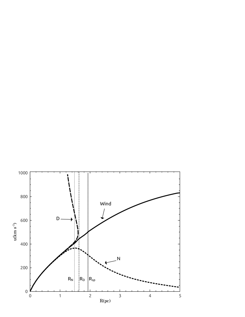
Figure 1: Possible integral curves. The value of the central temperature selects the type of the integral curve. If the central temperature is large, the integral curve reaches the maximum radius $r=R_{D}$ (vertical dashed line), where the denominator in equation (12) changes sign and the velocity becomes supersonic. The integral curve then goes back towards the center. This is non physical double value solution. If the central temperature is low, the integral curve reaches the maximum velocity at $r=R_{N}$ (vertical dotted line), where the numerator in equation (12) changes the sign. The velocity then drops with distance to the star cluster center. The velocity is always subsonic in this case. This is known as a “breeze” solution (e.g. Bjorkman, 1995). The wind solution is the unique solution, which passes by the singular point at $r=R_{sp}$ (vertical solid line), where both, the numerator and denominator in equation (12) vanish and the flow becomes supersonic for larger radius.

The wind solution is the unique solution, which passes through the singular point, where both, the numerator and the denominator in equation (12), vanish and the subsonic flow in the inner zone, $r<R_{sp}$, becomes supersonic at $r>R_{sp}$. This outer boundary condition i.e. that the integral curve must pass through the singular point, allows one to select the value of the central temperature which leads to the wind solution, and also defines the singular point position.

5 The integration procedure

As shown in Figure 1, there are three possible types of integral curves. We will call them N-type, D-type and wind-type solutions, as indicated in Figure 1. The N-type solution is subsonic everywhere. In this case the velocity grows monotonically with distance from the star cluster center until it reaches a maximum value when the numerator in equation (12) vanishes. For larger distances the numerator in (12) becomes negative, however the denominator does not, and thus the velocity drops and the flow remains always subsonic. The D-type solution passes the sonic point at some distance from the center. At this point the denominator in (12) vanishes, however the numerator does not. The integral curve then reaches the maximum radius and then turns back towards the center as the velocity grows. Note that one can easily obtain this solution, if the velocity is used instead of the radius as the independent variable. The wind-type solution is the only solution, which meets the singular point where both, the numerator and denominator in the equation of motion vanish.

Which type of the integral curve is selected, depends on the value of the central temperature. D-type solution occurs when the central temperature exceeds that which results into the wind-type solution. N-type solution occurs in the opposite case. This allows to build up a simple iteration procedure, which allows one to obtain the central temperature and the position of the singular point for the wind-type solution. The procedure is based on the bisection method and includes three integrations with three different central temperatures, $T_{max}$, $T_{min}$ and $T_{A}=(T_{max}+T_{min})/2$ at each iteration step. The initial values of $T_{max}$ and $T_{min}$ must be selected in such a way that $T_{max}$ is larger and $T_{min}$ is smaller than the wind-type central temperature. The central temperature, $T_{c}$, for the wind-type solution is always between the values of $T_{max}$ and $T_{min}$: $T_{min}<T_{c}<T_{max}$. At the end of each iteration step, either $T_{max}$ or $T_{min}$ is replaced with $T_{A}$, what allows to narrow the interval for the wind central temperature and approach closer to the singular point. We usually stop iterations, when the position of the singular point is within an accuracy $\delta\leq 10^{-3}$, where $\delta=[(R_{A}-R_{min})^{2}+(R_{A}-R_{max})^{2}]^{1/2}/R_{A}$. $R_{max}$, $R_{min}$ and $R_{A}$ are the radii, at which the denominator or numerator in the equation of motion (12) vanishes in the solutions with central temperatures $T_{max}$, $T_{min}$ and $T_{A}$, respectively. This procedure allows one to obtain the value of the wind central temperature and to localize the position of the singular point with high accuracy.

However, it does not allow to pass through the singular point and obtain the runs of the hydrodynamic variables for $r\geq R_{sp}$. In order to extend integral curves outside of the singular radius $R_{sp}$ and complete the solution, one must know the values and the derivatives of the hydrodynamical variables in the singular point. We obtain these quantities from the condition that at the singular point both, the numerator and the denominator in equation (12) vanish and thus the velocity of the flow is equal to the local speed of sound, $u_{sp}=c_{sp}$ (see Appendix).

6 Results and discussion

In order to verify our model, we first compared our results with those obtained by Ji et al. (2006), who integrated numerically equations (7)-(9) assuming that the impact from radiative cooling is negligible. Ji et al. (2006) obtained the singular radius $R_{sp}=1.97$ pc for $R_{c}=0.48$ pc, ${\dot{M}}_{SC}=10^{-4}$  $\hbox{M}_{\odot}$  yr^-1 and $V_{A\infty}=1000$ km s^-1 (see section 4 and Figure 8 in their paper). The run of the wind velocity obtained with our code for such an input model is shown in Figure 1 by the solid line. It is very similar to that, obtained in the 1D simulations (note that Ji et al. normalized their radii to the singular radius, $R_{sp}$). The radius of the singular point in our calculations is $R_{sp}=1.94$ pc. This implies that in the quasi-adiabatic case our model is in excellent (about 1.5%) agreement with the 1D results of Ji et al. (2006).

Table 1: Reference models

Model	Core radius	Half-mass radius	Mechanical luminosity	Adiabatic terminal speed
	(pc)	(pc)	(erg s-1)	(km s-1)
(1)	(2)	(3)	(4)	(5)
A	1.0	2.67	$3\times 10^{40}$	1000
B	1.0	2.67	$3\times 10^{39}$	1000
C	1.0	2.67	$3\times 10^{41}$	1000

Figure 2 shows the results of the calculations for our three reference models presented in Table 1. The model clusters have the same core radius (1 pc) and adiabatic wind terminal speed (1000 km s^-1) but different mechanical luminosities: $L_{SC}=3\times 10^{40}$ erg s^-1, $L_{SC}=3\times 10^{39}$ erg s^-1 and $L_{SC}=3\times 10^{41}$ erg s^-1. These mechanical luminosities correspond to young stellar clusters with masses about $M_{SC}=10^{6}$ $\hbox{M}_{\odot}$, $10^{5}$ $\hbox{M}_{\odot}$  and $10^{7}$ $\hbox{M}_{\odot}$, respectively. The distributions of velocity, temperature, density and pressure are shown in panels a, b, c and d, respectively. The solid, dotted and dashed lines correspond to cases A, B and C. In all cases the flow velocity near the center grows almost linearly with radius, passes the singular point at about 4 pc distance from the center and then gradually approaches the terminal speed value. The wind velocities are almost identical in the quasi-adiabatic models A and B (solid and dotted lines, respectively).

The impact of strong radiative cooling is noticeable in the most energetic case C. In this case the terminal wind velocity is smaller than in the cases A and B because radiative cooling reduces the amount of thermal energy in the central zone, that results into a smaller wind energy, and thus smaller terminal speed. The impact from radiative cooling is best noticed in the radial profiles of temperature and thermal pressure (panels b and d, respectively). In the quasi-adiabatic cases A and B the temperature drops slowly with distance from the star cluster core showing almost un-distinguishable distributions (solid and dotted lines in panel b). In model C the temperature profile is different. The temperature deviates from the quasi-adiabatic profile significantly already at about ten times the core radius and then drops rapidly to the lower permitted value, of about $10^{4}$ K, at about 35 pc from the center. This leads to the fast decrease in the thermal pressure (panel d) which drops more than an order of magnitude at this distance. Note, that thermal pressure always drops rapidly with distance from the star cluster center in the free wind region. Figure 2 shows also that the central pressure grows with the star cluster mass/power. This is also the case for the central density (see panel c). However, radiative cooling does not affect the density distribution significantly even in the most powerful case C (panel c).

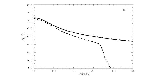
Figure 2: The stationary wind solution. Panels a, b, c and d present the wind velocity, temperature, density and pressure, respectively. Solid, dotted and dashed lines present the results of the calculations for models A, B and C. Thick and thin lines in panel d display the thermal and ram pressure, respectively.

The value of $V_{A\infty}$ parameterizes the ratio of the star cluster mechanical luminosity to the mass deposition rate. Both parameters, $L_{SC}$ and ${\dot{M}}_{SC}$, vary as the cluster evolves (e.g. Leitherer et al., 1999). Beside this, the flow may be mass loaded by the gas left over from star formation (Stevens & Hartwell, 2003; Silich et al., 2010). Figure 3 presents the results of the calculations for three different values of this parameter: $V_{A\infty}=1000$ km s^-1, $V_{A\infty}=750$ km s^-1 and $V_{A\infty}=2000$ km s^-1 (solid, dashed and dotted lines, respectively). The rest of the input parameters in this set of models are the same as in the reference model A: $L_{SC}=3\times 10^{40}$ erg s^-1 and $R_{c}=1$ pc. The calculated wind central temperature (see panel b) increases for larger $V_{A\infty}$ as it is also the case in the non-radiative solution (see Cantó et al. 2000). The calculated wind terminal speed is similar to the adiabatic value when $V_{A\infty}$ parameter is large. However, in the low velocity case, $V_{A\infty}=750$ km s^-1, the difference between the adiabatic and the calculated terminal speeds is noticeable. This is because the density in the wind, $\rho={\dot{M}}(r)/4\pi r^{2}u(r)$, is larger if the selected adiabatic wind terminal speed is smaller (Figure 3, panel c) that leads to a stronger radiative cooling. Strong radiative cooling removes a fraction of the deposited energy and thus decreases the flux of mechanical energy and consequently the wind terminal speed. Indeed, in the quasi-adiabatic cases with $V_{A\infty}=2000$ km s^-1 and $V_{A\infty}=1000$ km s^-1 the amount of radiated energy is negligible, but it reaches about $14\%$ of the deposited energy in the model with $V_{A\infty}=750$ km s^-1. In this case, radiative cooling leads to the rapid decrease in the temperature distribution at about 35 pc distance from the star cluster center as it is also the case in the reference model C. This results into the sharp drop of thermal pressure at the same distance (see panel d). Nevertheless, the position of the singular point, $R_{sp}$, remains about the same, $R_{sp}\approx 4$ pc.

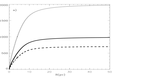
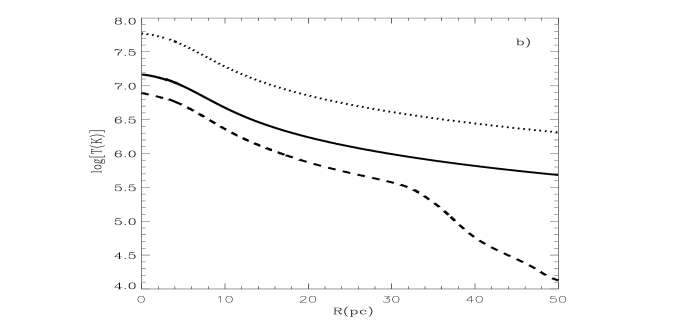
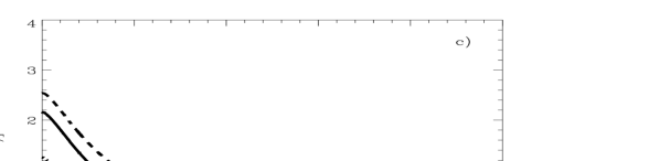
Figure 3: The results of the calculations for models with different $V_{A\infty}$. Panels a, b, c and d present the wind velocity, temperature, density and pressure, respectively. Solid, dotted and dashed lines present the results of the calculations for models with $V_{A\infty}=1000$ km s^-1, $V_{A\infty}=2000$ km s^-1 and $V_{A\infty}=750$ km s^-1, respectively. Thick and thin lines in panel d display the thermal and ram pressure, respectively.

Finally, Figure 4 shows how the distributions of the hydrodynamical variables change with the star cluster core radius. This figure displays the resulting velocity, temperature, density and pressure profiles for clusters which have the same mechanical luminosity ($L_{SC}=3\times 10^{40}$ erg s^-1) and adiabatic wind terminal speed ($V_{A\infty}=1000$ km s^-1), but different core radii: $R_{c}=1$ pc, $R_{c}=5$ pc and $R_{c}=0.2$ pc (solid, dotted and dashed lines, respectively). Certainly, the speed of the wind grows faster when the cluster is more compact, as it is shown in panel a. The central temperatures are the same in all cases. However, the temperature profiles are different. In the case with a larger core radius the flow is quasi-adiabatic and the temperature drops slowly with radius. On the other hand, the most compact model with $R_{c}=0.2$ pc is strongly affected by radiative cooling (dashed line in panel b). In this case the temperature drops rapidly and reaches the $10^{4}$ K value at about 17 pc distance from the center. One can also notice the effects of strong radiative cooling on panel d, which displays the calculated star cluster wind thermal and ram pressure profiles. The value of the core radius affects also the wind central density which grows for smaller core radius, as shown in panel c.

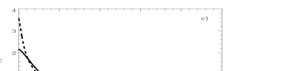
Figure 4: The results of the calculations for models with different $R_{c}$. Panels a, b, c and d present the wind velocity, temperature, density and pressure, respectively. Solid, dotted and dashed lines present the results of the calculations for models with $R_{c}=1$ pc, $R_{c}=5$ pc and $R_{c}=0.2$ pc, respectively. Thick and thin lines in panel d display the thermal and ram pressure, respectively.

7 The catastrophic cooling regime

The density in the wind grows with the star cluster mechanical luminosity/mass. It also increases if the wind is mass loaded (as the adiabatic wind terminal speed is smaller) or if the cluster is more compact (for a smaller $R_{c}$). In all these cases the impact of radiative cooling on the flow hydrodynamics becomes progressively more significant, as discussed in the previous section. The turn-off point in the temperature distribution moves towards the star cluster center and the temperature rapidly drops to the $10^{4}$ K value. At larger radii it falls even to lower values because of the gas expansion. Hereafter we will assume that the outflow is photoionized by young massive stars and thus the wind becomes isothermal as soon as the temperature reaches the $10^{4}$ K value. Outwards of this radius we replace the set of the main equations (12)- (14) with equations describing isothermal flows:

$$\frac{{\rm d}u}{{\rm d}r}=\frac{2\rho c^{2}/\gamma r-(1+c^{2}/\gamma u^{2})q_{m}u}{(1-c^{2}/\gamma u^{2})\rho u}$$ (19)

$$\rho=\frac{2q_{m0}R_{c}^{3}}{r^{2}u}\left[1-\left(1+\frac{r}{R_{c}}+\frac{1}{2}\frac{r^{2}}{R^{2}_{c}}\right)\exp(-r/R_{c})\right]\,,$$ (20)

where the sound speed, $c^{2}=\gamma kT/\mu_{a}$, is constant and the temperature is $T=10^{4}$ K. The thermal pressure then is: $P=\rho c^{2}/\gamma$. However, in the numeric code we obtain thermal pressure by integrating the differential equation

$$\frac{{\rm d}P}{{\rm d}r}=\frac{c^{2}}{\gamma}\left(\frac{q_{m}}{u}-\frac{\rho}{u}\frac{{\rm d}u}{{\rm d}r}-\frac{2\rho}{r}\right)\,.$$ (21)

This allows to minimize changes in the numerical code, when the transition occurs from the radiative to the isothermal regime.

In the catastrophic cooling regime the singular point detaches from its quasi-adiabatic position and then rapidly moves towards the center. One can note that in this respect our solution is similar to that, found by Bisnovatyi-Kogan & Blinnikov (1980) for the accretion of the pre-heated gas onto a neutron star. In the later case the singular point is also located far away from the center, near the Bondi radius, if the accretion rate is low and the pre-heating of the accretion flow is small. However, when the accretion rate grows, the catastrophic heating regime sets in. The singular point detaches then from the Bondi radius and moves rapidly towards the neutron star surface.

Figure 5 presents an example of the catastrophic cooling regime. In this case the star cluster core radius and the adiabatic wind terminal speed are the same as in our reference model A, but the mechanical luminosity of the cluster is two orders of magnitude larger: $L_{SC}=3\times 10^{42}$ erg s^-1.

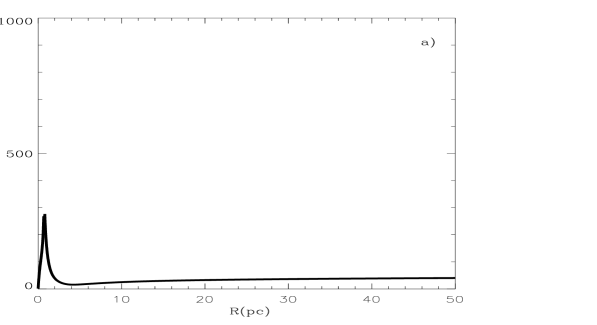
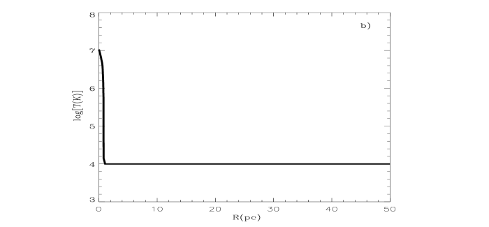
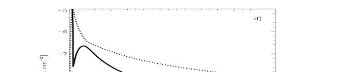
Figure 5: Catastrophic cooling regime. The distribution of the hydrodynamic variables in the model with $L_{SC}=3\times 10^{42}$ erg s^-1, $R_{c}=1$ pc and $V_{A\infty}=1000$ km s^-1. Panels a, b, c and d present the wind velocity, temperature, density and pressure, respectively. Solid and dotted lines in panel d display the thermal and the ram pressure, respectively.

The singular point moves then inside the core radius, to $R_{sp}=0.66$ pc distance from the star cluster center. The maximum flow velocity is much smaller, than in the quasi-adiabatic case. It reaches only about 300 km s^-1 at the singular point (see panel a in Figure 5). The flow slows down then to about 16 km s^-1 being loaded with the newly re-inserted matter with zero initial momentum. In this regime the last term in equation (8) dominates over the thermal pressure gradient. The velocity then increases slowly because in the isothermal regime the ionizing photons heat up and dump additional energy to the flow. The density grows in the region, where the wind slows down, and then decreases again in the isothermal wind region. The temperature drops abruptly to the $10^{4}$ K value when the flow passes the singular point. The thermal pressure also drops just after the singular point and then increases in the region where the density grows up and the temperature reaches a constant value.

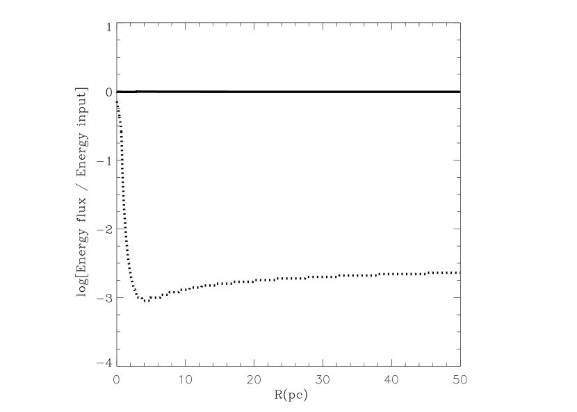
Figure 6: The catastrophic cooling regime. The ratio of the mechanical energy flux to the energy input rate as a function of radius. The solid and dotted lines present the results of the calculations for the reference model A and the model with the same core radius and adiabatic wind terminal speed, but two orders of magnitude larger mechanical luminosity, respectively.

In the case under consideration the radiative losses of energy are catastrophic indeed. Figure 6 shows the ratio of the energy flux through the surface with radius $r$: $L_{w}(r)=4\pi\rho u(r)r^{2}(u^{2}(r)/2+H(r))$, where $H$ is the enthalpy, to the mechanical energy input rate inside the enclosed volume: $L_{SC}(r)=L_{SC}[1-(1+r/R_{c}+r^{2}/2R^{2}_{c})\exp(-r/R_{c})]$. The solid line in Figure 6 displays this ratio for the reference model A, whereas the dotted one shows the same ratio in the catastrophic cooling regime. In the catastrophic cooling regime $L_{w}(r)/L_{SC}(r)$ drops very rapidly to about $10^{-3}$ value, whereas in the quasi-adiabatic model A it is close to unity at any distance from the star cluster center. This implies that in the extreme case, here discussed, the star cluster wind carries away only about 0.1% of the deposited mechanical energy. The rest is radiated away because of strong radiative cooling.

Note, that the catastrophic cooling regime also sets in if one provides simulations for less energetic, but more compact clusters, and in the case of less energetic models with smaller adiabatic wind terminal speed parameter. In this regime the terminal wind velocity is small and may fall below the escape velocity. In this case a fraction of the re-inserted matter might remain gravitationally bound and accumulate inside the star cluster volume. Thus, in the catastrophic cooling regime the gravitational pull from the cluster becomes an important factor (Silich et al., 2010), which should be included into the model. The impact that gravitational field of the cluster provides on the flow will be discussed in a future communication.

8 Comparison with homogeneous model predictions

In this section we confront the predictions from the exponential model with those, obtained under the assumption that stars are homogeneously distributed within the star cluster volume. Throughout this section we will assume that the two clusters have the same mass and their winds the same adiabatic terminal speed, but different, either exponential or homogeneous, stellar mass distributions. As shown in section 6 and in our prior papers, the distribution of the hydrodynamical variables and thus the observational manifistations of star cluster winds strongly depend on the characteristic space scale of the stellar mass distribution: the core radius, $R_{c}$, in models with an exponential stellar density distribution and on the star cluster radius, $R_{SC}$, in models with a homogeneous stellar distribution. Thus, one has to link these two parameters in order to compare the models. This could be done in different ways. For example, Ji et al. (2006) compared two models assuming that in both cases the singular points are located at the same distance from the star cluster center. One can instead use the same half-mass radius $R_{hm}$ (e.g. Portegies Zwart et al., 2010). Specifically, here we assume equally massive clusters with different stellar mass distributions but with the same half-mass radii: $R_{hme}=R_{hmh}$, where the half-mass radius is $R_{hme}=2.67R_{c}$ in the exponential case and $R_{hmh}=0.79R_{SC}$ in models with a homogeneous mass distribution. The relation between the core radius $R_{c}$ and the star cluster radius $R_{SC}$ then is:

$$R_{c}\approx 0.3R_{SC}.$$ (22)

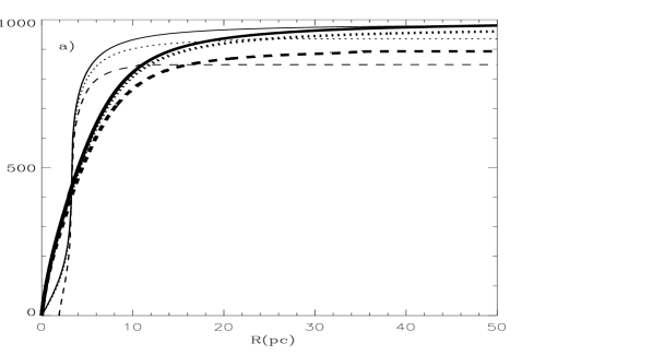
Figure 7: The comparison of the exponential and the homogeneous model predictions. Panels a, b, c and d present the distributions of the wind velocity, temperature, density and thermal pressure, respectively. Solid, dotted and dashed lines display the results of the calculations for models with $L_{SC}=3\times 10^{40}$ erg s^-1, $L_{SC}=10^{41}$ erg s^-1 and $L_{SC}=3\times 10^{41}$ erg s^-1. Thick and thin lines show the distributions of the hydrodynamical variables in the case with exponential and homogeneous mass distribution, respectively. It was assumed that the adiabatic wind terminal speed parameter is the same in all cases: $V_{A\infty}=1000$ km s^-1.

We present three cases: our reference models A and B and an intermediate model with an energy input rate $L_{SC}=10^{41}$ erg s^-1 and assume that in each case the mass distribution may be either exponential, or homogeneous. The results of the calculations are presented in Figure 7. Solid, dotted and dashed lines in Figure 7 display the results of the calculations for models with $L_{SC}=3\times 10^{40}$ erg s^-1, $L_{SC}=10^{41}$ erg s^-1 and $L_{SC}=3\times 10^{41}$ erg s^-1, respectively. Thick and thin lines show the distributions of the hydrodynamical variables in the case with an exponential and a homogeneous mass distribution, respectively. One can note, that models with an exponential stellar mass distribution are less affected by radiative losses of energy. Indeed, in the calculations with homogeneous mass distribution the temperature and the thermal pressure already deviate significantly from the quasi-adiabatic profiles when the star cluster mechanical luminosity is $L_{SC}=10^{41}$ erg s^-1 whereas in the exponential case are not (compare thin and thick dotted lines in panels b and d). The mechanical energy input rate in the most energetic homogeneous model with $L_{SC}=3\times 10^{41}$ erg s^-1 exceeds the threshold value (see Figure 2 in Tenorio-Tagle et al., 2007). In this case the stagnation point (the point where the wind velocity is 0 km s^-1) shifts from the center to $R_{st}=1.9$ pc and the shock-heated plasma becomes thermally unstable within the central zone with $r\leq R_{st}$ (Wünsch et al., 2008). We did not find a similar bimodal regime in calculations with an exponential stellar distribution. In these cases, the faster drop in density inhibits catastrophic cooling in the center. The two models are quite different in this respect. In the models with a homogeneous star distribution, the position of the singular point is fixed at $r=R_{SC}$ but the stagnation point may move from the center due to catastrophic cooling. In the models with an exponential stellar mass distribution it is quite the opposite: the stagnation point remains always at the center, whereas the singular point may detach from its quasi-adiabatic position and move closer towards the center. Thus the definition of the threshold mechanical luminosity as the mechanical luminosity above which the stagnation point moves from the star cluster center and the central zone becomes thermally unstable does not occur in models with an exponential stellar mass distribution. However, the flow may be thermally unstable outside of the singular point in this case. This will be thoroughly discussed in a forthcoming communication.

Figure 8: The distribution of the X-ray emission along the star cluster wind. The solid and dotted lines show the distribution of the X-ray luminosity $\epsilon_{X}$ (see the text) along the star cluster wind in the case of the exponential and the homogeneous stellar mass distribution, respectively. Note, that both luminosities are normalized to the total homogeneous wind luminosity, $L_{Xtot}=8.1\times 10^{38}$ erg s^-1, and that X-ray emission is slightly more concentrated in the case with homogeneous stellar mass distribution.

Diffuse X-ray emission has been detected from many young stellar clusters and their associated HII regions (e.g. Moffat et al., 2002; Law & Yusef-Zadeh, 2004, see the review of the resent results in Townsley et al., 2011). Cantó et al. (2000), Raga et al. (2001), Stevens & Hartwell (2003), Silich et al. (2005), Rockefeller et al. (2005) and Rodríguez-González et al. (2007) suggested that the observed diffuse X-ray emission manifests the hot, shock-heated star cluster winds. The contribution from the hot massive stars to the observed X-ray emission has been discussed by Oskinova (2005). The X-ray luminosity of the star cluster wind then is:

$$L_{X}=4\pi\int_{0}^{R_{out}}r^{2}n_{e}n_{i}\Lambda_{X}(T,Z){\rm d}r,$$ (23)

where $n_{e}(r)$ and $n_{i}(r)$ are the electron and ion number densities, $\Lambda_{X}(Z,T)$ is the X-ray emissivity used by Strickland & Stevens (2000) and $R_{out}$ marks either the location of the outer wind driven shock, or the X-ray cut-off radius (the radius where the temperature in the wind drops below $T_{cut}\approx 5\times 10^{5}$K). We integrate equation (23) numerically using the temperature and density profiles obtained from calculations with either exponential or homogeneous stellar mass distribution, assuming that $n_{e}=n_{i}=\rho(r)/\mu_{i}$, where $\mu_{i}=14/11m_{H}$ is the ion number density. We found that the exponential model predicts a slightly smaller (within a factor of two) X-ray luminosity. For example, when the mechanical luminosity of the cluster is $L_{SC}=3\times 10^{40}$ erg s^-1 (model A), the calculations with exponential stellar mass distribution predict the total 0.3 keV - 8.0 keV wind luminosity $L_{Xtot}=5.2\times 10^{38}$ erg s^-1 whereas the homogeneous model leads to $L_{Xtot}=8.1\times 10^{38}$ erg s^-1. When $L_{SC}=10^{41}$ erg s^-1, the exponential model predicts $L_{Xtot}=6.1\times 10^{39}$ erg s^-1 whereas the homogeneous one $L_{Xtot}=1.0\times 10^{40}$ erg s^-1. We cannot compare the X-ray luminosities in the most energetic case C because the central zone in the model with homogeneous stellar mass distribution is thermally unstable and the distributions of the hydrodynamical variables inside this zone cannot be obtained in the semi-analytic calculations. Figure 8 compares the distributions of the X-ray emission along the wind, $\epsilon_{X}=[L_{Xtot}-L_{X}(r)]/L_{Xtot}$, in the case when the star cluster mechanical luminosity is $L_{SC}=3\times 10^{40}$ erg s^-1. Very similar results were obtained in the calculations where instead of $R_{hme}=R_{hmh}$ the same singular radius, as suggested by Ji et al. (2006) was used for the two stellar mass distribution models.

9 Summary

Here we present, for the first time, a radiative semi-analytic solution for steady state, spherically-symmetric winds driven by stellar clusters with an exponential stellar density distribution. The method, here developed, improves previous calculations provided for stellar clusters with a given size and a homogeneous stellar density distribution and thus leads to more reliable hydrodynamic predictions. It may be easily extended to clusters with other stellar density distributions.

In our model, unlike in most previous calculations, the position of the singular point, $R_{sp}$, where the transition from the subsonic to the supersonic flow occurs, is not associated with the star cluster edge, but calculated from the condition that the integral curve must pass through the singular point. When radiative losses of energy are negligible, the singular radius is always about $R_{sp}\approx 4R_{c}$, where $R_{c}$ is the star cluster core radius, irrespective of the other star cluster parameters. This is not the case in the catastrophic cooling regime, when the temperature drops abruptly at a short distance from the star cluster center and the transition from the subsonic to the supersonic regime occurs at the much smaller distance from the star cluster center.

Radiative cooling becomes a significant factor when the cluster is very energetic/massive, compact, or the adiabatic wind terminal speed parameter, $V_{A\infty}=(2L_{SC}/{\dot{M}}_{SC})^{1/2}$, is small. In the catastrophic cooling regime outflows carry away of the star cluster region only a small fraction of the deposited mechanical energy. The gravitationally bound, partially ionized nebulae may be formed then, if the photoionized gas cannot escape the gravitational well of the cluster. On the other hand, the low mass clusters with small energy input rates and large radii drive quasi-adiabatic winds. In these cases our results show an excellent agreement with the results of non-radiative 1D numerical simulations.

The star cluster driven wind model presented here may be applied to many problems, which are currently discussed in the literature. Such, as the star cluster diffuse X-ray emission, the origin of compact HII regions, which are frequently detected around young massive clusters and the origin of the low-ionization line emission in the starburst driven galactic-scale outflows. We will address some of them in a future communication.

Appendix

In order to obtain the flow velocity, pressure, their derivatives, and also the density and the temperature at the singular point, one has to use the condition that at this point the numerator and the denominator in equation (12) vanish. The denominator in equation (12) vanishes when the wind velocity reaches the local speed of sound and thus: $u_{sp}=c_{sp}$. The density in the singular point (see equation 14) then is:

$$\rho_{sp}=\frac{2q_{m0}R_{c}^{3}}{R^{2}_{sp}c_{sp}}\left[1-\left(1+\frac{R_{sp}}{R_{c}}+\frac{1}{2}\frac{R_{sp}^{2}}{R^{2}_{c}}\right)\exp(-R_{sp}/R_{c})\right]\,$$ (A1)

The second condition, that the numerator in equation (12) vanishes, then yields:

$$c^{4}_{sp}-2F_{1}(R_{sp})c^{2}_{sp}+F_{2}(R_{sp})\Lambda(T_{sp},Z)=0\,,$$ (A2)

where functions $F_{1}$ and $F_{2}$ are:

$$F_{1}=\frac{(\gamma-1)}{4F_{3}(R_{sp})}V^{2}_{A\infty}\exp(-R_{sp}/R_{c})\,,$$ (A3)

$$F_{2}=\frac{4(\gamma-1)q_{m0}R_{c}^{6}}{\mu^{2}_{i}R^{4}_{sp}F_{3}(R_{sp})}\left[1-\left(1+\frac{R_{sp}}{R_{c}}+\frac{1}{2}\frac{R_{sp}^{2}}{R^{2}_{c}}\right)\exp(-R_{sp}/R_{c})\right]^{2}\,,$$ (A4)

and

$$F_{3}=4\left(\frac{R_{c}}{R_{sp}}\right)^{3}(1-\exp(-R_{sp}/R_{c}))-$$

$$\left[\frac{\gamma+1}{2}+4\left(\frac{R_{c}}{R_{sp}}\right)^{2}\left(1+\frac{R_{sp}}{2R_{c}}\right)\right]\exp(-R_{sp}/R_{c})\,,$$ (A5)

$\mu_{i}=14/11m_{H}$ is the mean mass per ion.

This nonlinear algebraic equation defines the temperature at the singular point, $T_{sp}$, if $R_{sp}$ is known. One can present equation (A2) in the dimensionless form and then solve it numerically:

$$FA=1-2F_{1}(R_{sp})c^{-2}_{sp}+F_{2}(R_{sp})\Lambda(T_{sp},Z)c^{-4}_{sp}=0.$$ (A6)

Equation (A6) may have one, two, or have nor real roots as it is shown in Figure 9, which displays function FA tabulated at $R_{sp}=4$ pc radius for three different values of the star cluster mechanical luminosity: $L_{SC}=3\times 10^{40}$ erg s^-1, $L_{SC}=3\times 10^{41}$ erg s^-1 and $L_{SC}=3\times 10^{42}$ erg s^-1 - solid, dotted and dashed lines, respectively. The proper solution of equation (A6) is selected from the condition, that segments of the integral curve obtained by the outward integration from the star cluster center and by the inward integration from the singular point match in an interior radius $0<R_{fit}<R_{sp}$. Note, that one has to obtain the position of the singular point, $R_{sp}$, by iterations as it is described in Section 5.

Having the value of $T_{sp}$, one can obtain the velocity in the singular point, which is: $u_{sp}=c_{sp}$. The density in the singular point yields from equation (A1), the pressure then is: $P_{sp}=\rho_{sp}c^{2}_{sp}/\gamma$. Thus, one can obtain the values of all hydrodynamic variables in the singular point solving the nonlinear algebraic equation (A6). The value of the singular radius, $R_{sp}$, is obtained by iterations, as explained in section 5.

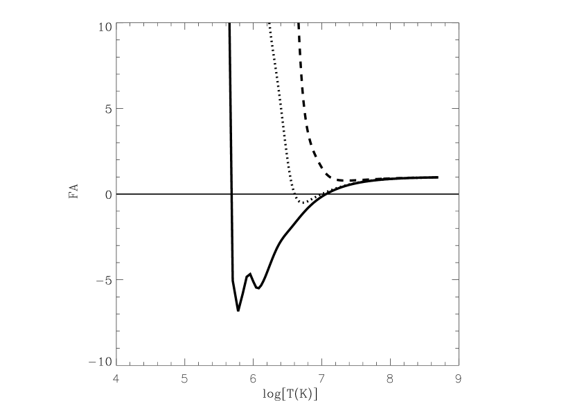
Figure 9: Different roots of equation (A6). Solid, dashed and dotted lines display function FA tabulated at $R_{sp}=4$ pc for three different mechanical luminosities: $L_{SC}=3\times 10^{40}$ erg s^-1, $L_{SC}=3\times 10^{41}$ erg s^-1 and $L_{SC}=3\times 10^{42}$ erg s^-1, respectively.

In order to obtain the derivative of velocity in the singular point, one can use the L’Hopital’s rule. The derivatives of numerator and denominator of equation (12) over radius are:

$$\frac{{\rm d}N}{{\rm d}r}=\frac{\partial N}{\partial r}+\frac{\partial N}{\partial u}\frac{{\rm d}u}{{\rm d}r}+\frac{\partial N}{\partial c^{2}}\frac{{\rm d}c^{2}}{{\rm d}r}+\frac{\partial N}{\partial T}\frac{{\rm d}T}{{\rm d}r}+\frac{\partial N}{\partial\rho}\frac{{\rm d}\rho}{{\rm d}r}=F_{5}\frac{{\rm d}u}{{\rm d}r}+F_{6}+\frac{\partial N}{\partial r}\,,$$ (A7)

$$\frac{{\rm d}D}{{\rm d}r}=\frac{\partial D}{\partial u}\frac{{\rm d}u}{{\rm d}r}+\frac{\partial D}{\partial c^{2}}\frac{{\rm d}c^{2}}{{\rm d}r}=-(\gamma+1)c\left(\frac{{\rm d}u}{{\rm d}r}+\frac{q_{m}}{\rho}\right)+\frac{2c^{2}}{r}\,,$$ (A8)

where functions $N$, $D$, $\partial{N}/\partial{r}$, $F_{5}$ and $F_{6}$ are:

$$N(r,u,\rho,c,T)=(\gamma-1)(q_{e}-Q)-4q_{m0}c^{2}(R_{c}/r)^{3}+$$

$$q_{m}[(\gamma+1)u^{2}/2+4c^{2}(R_{c}/r)^{3}(1+r/R_{c}+(r/R_{c})^{2}/2)]\,,$$ (A9)

$$D(u,c)=c^{2}-u^{2}\,$$ (A10)

$$\frac{\partial N}{\partial r}=-\frac{1}{R_{c}}\left[(\gamma-1)q_{e}+4q_{m0}c^{2}\left(\frac{R_{c}}{r}\right)^{3}\left[\exp(-r/R_{c})-\frac{3R_{c}}{r}(1-\exp(-r/R_{c}))\right]\right.+$$

$$\left.4q_{m}c^{2}\left[\frac{\gamma+1}{8}+2\left(\frac{R_{c}}{r}\right)^{3}+\frac{3}{2}\left(\frac{R_{c}}{r}\right)^{2}+\frac{1}{2}\frac{R_{c}}{r}\right]\right]\,,$$ (A11)

$$F_{5}=(1-\gamma)cF_{4}+(1+\gamma)q_{m}c+2(\gamma-1)\rho^{2}\Lambda/c\mu^{2}_{i}$$ (A12)

$$F_{6}=\frac{2(\gamma-1)\Lambda\rho^{2}}{\mu^{2}_{i}c}\left(\frac{2c}{r}-\frac{q_{m}}{\rho}\right)-\left[\frac{(\gamma+1)q_{m}c}{\rho}-\frac{2c^{2}}{r}\right]F_{4}\,,$$ (A13)

and

$$F_{4}=\frac{1-\gamma}{\gamma}\frac{\rho^{2}}{\mu_{i}k}\frac{\partial\Lambda}{\partial T}+$$

$$4q_{m0}\left(\frac{R_{c}}{r}\right)^{2}\left[\left(1+\frac{r}{2R_{c}}\right)\exp(-r/R_{c})-(1-\exp(-r/R_{c}))\frac{R_{c}}{r}\right]\,.$$ (A14)

One can obtain then the derivative of the wind velocity (and thus the derivative of the thermal pressure) at the singular point substituting relations (A7) and (A8) into equation (12) and keeping in mind that at the singular point $u_{sp}=c_{sp}$. This leads to a quadratic algebraic equation:

$$\left(\frac{{\rm d}u}{{\rm d}r}\right)^{2}-2F_{7}\frac{{\rm d}u}{{\rm d}r}+F_{8}=0\,,$$ (A15)

where functions $F_{7}$ and $F_{8}$ are:

$$F_{7}=\left[2\rho c^{2}/r-(\gamma+1)cq_{m}-F_{5}\right]/2(\gamma+1)c\rho\,,$$ (A16)

$$F_{8}=[F_{6}+\partial{N}/\partial{r}]/[(\gamma+1)c\rho]\,.$$ (A17)

The root of equation (A15), which leads to the positive derivative ${\rm d}{u}/{\rm d}{r}$ at the singular point, is used in the calculations.

References

- Bisnovatyi-Kogan & Blinnikov (1980) Bisnovatyi-Kogan, G. S. & Blinnikov, S. I. 1980, MNRAS, 191, 711
- Bjorkman (1995) Bjorkman, J. E. 1995, ApJ, 453, 369
- Böker et al. (2004) Böker, T., Sarzi, M., McLaughlin, D. E., et al. 2004, AJ, 127, 105
- Cantó et al. (2000) Cantó, J., Raga, A. C., & Rodríguez, L. F. 2000, ApJ, 536, 896
- Chevalier (1992) Chevalier, R. A. 1992, ApJ Let, 397, L39
- Chevalier & Clegg (1985) Chevalier, R. A. & Clegg, A. W. 1985, Nature, 317, 44
- de Grijs (2010) de Grijs, R. 2010, Royal Society of London Philosophical Transactions Series A, 368, 693
- Heckman et al. (1990) Heckman, T. M., Armus, L., & Miley, G. K. 1990, ApJS, 74, 833
- Ji et al. (2006) Ji, L., Wang, Q. D., & Kwan, J. 2006, MNRAS, 372, 497
- Johnson & Axford (1971) Johnson, H. E. & Axford, W. I. 1971, ApJ, 165, 381
- Law & Yusef-Zadeh (2004) Law, C. & Yusef-Zadeh, F. 2004, ApJ, 611, 858
- Leitherer et al. (1999) Leitherer, C., Schaerer, D., Goldader, J. D., et al. 1999, ApJS, 123, 3
- Marlowe et al. (1995) Marlowe, A. T., Heckman, T. M., Wyse, R. F. G., & Schommer, R. 1995, ApJ, 438, 563
- Moffat et al. (2002) Moffat, A. F. J., Corcoran, M. F., Stevens, I. R., et al. 2002, ApJ, 573, 191
- Oskinova (2005) Oskinova, L. M. 2005, MNRAS, 361, 679
- Portegies Zwart et al. (2010) Portegies Zwart, S. F., McMillan, S. L. W., & Gieles, M. 2010, ARA & A, 48, 431
- Raga et al. (2001) Raga, A. C., Velázquez, P. F., Cantó, J., Masciadri, E., & Rodríguez, L. F. 2001, ApJ Let, 559, L33
- Rockefeller et al. (2005) Rockefeller, G., Fryer, C. L., Melia, F., & Wang, Q. D. 2005, ApJ, 623, 171
- Rodríguez-González et al. (2007) Rodríguez-González, A., Cantó, J., Esquivel, A., Raga, A. C., & Velázquez, P. F. 2007, MNRAS, 380, 1198
- Rupke et al. (2005) Rupke, D. S., Veilleux, S., & Sanders, D. B. 2005, ApJS, 160, 87
- Sarazin & White (1987) Sarazin, C. L. & White, III, R. E. 1987, ApJ, 320, 32
- Silich et al. (2005) Silich, S., Tenorio-Tagle, G., & Añorve-Zeferino, G. A. 2005, ApJ, 635, 1116
- Silich et al. (2003) Silich, S., Tenorio-Tagle, G., & Muñoz-Tuñón, C. 2003, ApJ, 590, 791
- Silich et al. (2010) Silich, S., Tenorio-Tagle, G., Muñoz-Tuñón, C., et al. 2010, ApJ, 711, 25
- Silich et al. (2004) Silich, S., Tenorio-Tagle, G., & Rodríguez-González, A. 2004, ApJ, 610, 226
- Stevens & Hartwell (2003) Stevens, I. R. & Hartwell, J. M. 2003, MNRAS, 339, 280
- Strickland & Stevens (2000) Strickland, D. K. & Stevens, I. R. 2000, MNRAS, 314, 511
- Tenorio-Tagle et al. (2007) Tenorio-Tagle, G., Wünsch, R., Silich, S., & Palouš, J. 2007, ApJ, 658, 1196
- Townsley et al. (2011) Townsley, L. K., Broos, P. S., Chu, Y.-H., et al. 2011, ApJS, 194, 16
- Turner (2009) Turner, J. L. 2009, Astrophysics in the Next Decade, ed. Thronson, H. A., Stiavelli, M., & Tielens, A., p.215
- Veilleux et al. (2005) Veilleux, S., Cecil, G., & Bland-Hawthorn, J. 2005, ARA & A, 43, 769
- Walcher et al. (2005) Walcher, C. J., van der Marel, R. P., McLaughlin, D., et al. 2005, ApJ, 618, 237
- Westmoquette et al. (2008) Westmoquette, M. S., Smith, L. J., & Gallagher, J. S. 2008, MNRAS, 383, 864
- Wünsch et al. (2011) Wünsch, R., Silich, S., Palous, J., Tenorio-Tagle, G., & Munoz-Tunon, C. 2011, ApJ, 740, 75
- Wünsch et al. (2008) Wünsch, R., Tenorio-Tagle, G., Palouš, J., & Silich, S. 2008, ApJ, 683, 683