Slow interaction ramps in trapped many-particle systems: universal deviations from adiabaticity

Abstract

For harmonic-trapped atomic systems, we report system-independent non-adiabatic features in the response to interaction ramps. We provide results for several different systems in one, two, and three dimensions: bosonic and fermionic Hubbard models realized through optical lattices, a Bose-Einstein condensate, a fermionic superfluid and a fermi liquid. The deviation from adiabaticity is characterized through the heating or excitation energy produced during the ramp. We find that the dependence of the heat on the ramp time is sensitive to the ramp protocol but has aspects common to all systems considered. We explain these common features in terms of universal dynamics of the system size or cloud radius.

I Introduction

Adiabaticity is an essential and ubiquitous concept in quantum dynamics. In the current era of many novel non-equilibrium experimental possibilities, deviations from adiabaticity in slow parameter changes have attracted a lot of attention finiteRateQuenches_reviews ; Polovnikov_AdiabaticPertThy ; finiteRateQuenches_residualenergy ; EcksteinKollar_NJP2010 ; CanoviRossiniFazioSantoro_JSM09 ; MoeckelKehrein_NJP2010 ; DoraHaqueZarand_arxiv10 ; DziarmagaTylutki_arxiv11 ; Venumadhav_PRB2010 ; ramp_papers_finitesystems . The question of non-adiabaticity is of fundamental interest, but also has practical implications. Many experimental protocols involve adiabatically changing a parameter in order to reach a desired quantum state. Since non-adiabatic heating can rarely be completely avoided, it is essential to understand deviations from adiabaticity in slow ramps. While the effect of quantum critical points in the ramp path has been considered in much detail finiteRateQuenches_reviews ; Polovnikov_AdiabaticPertThy , settings for non-equilibrium experiments in isolated systems tend to be mesoscopic rather than macroscopic, without true quantum critical points. Understanding non-adiabatic ramps in finite quantum systems is therefore vital. Also, since cold atoms dominate experimental non-equilibrium studies, a harmonically trapped many-particle system is the most important paradigm today for studying quenches and ramps. A few studies of ramps in finite and trapped systems have appeared in the very recent literature Venumadhav_PRB2010 ; ramp_papers_finitesystems , indicating an emerging recognition of the importance of the adiabaticity issue in finite systems. In addition, in the past couple of years, reports of experimental investigations of finite-rate interaction ramps have started to appear, both in the continuum Salomon_BEC_ramp_2011 and in optical-lattices HungZhangGemelkeChin_PRL10 ; BakrPolletGreiner_Science2010 ; DeMarco_PRL11 , with harmonically trapped atoms.

In this work, we consider non-adiabatic ramps in several distinct interacting many-particle systems, confined in isotropic harmonic traps. In each case, we consider ramps of the interaction from an initial value $U_{\rm i}$ to a final value $U_{\rm f}$, occurring in time scale $\tau$. We focus on large but finite $\tau$ (near-adiabatic ramps). We study deviations from adiabaticity through the heating $Q$, which is the final energy at time $t\gg\tau$ minus the ground state energy of the final Hamiltonian. This quantity is also called the residual energy or excess excitation energy EcksteinKollar_NJP2010 ; CanoviRossiniFazioSantoro_JSM09 ; finiteRateQuenches_residualenergy ; Venumadhav_PRB2010 , and may be thought of as the “friction” due to imperfect adiabaticity Muga_delCampo_frictionless . The asymptotic form of $Q(\tau)$ is a quantitative characterization of minimal corrections to adiabaticity. Ref. DeMarco_PRL11 reports measurements of excess energies after ramps, which may be regarded as the first experimental approach to this quantity.

We find that the asymptotics of $Q(\tau)$ is common to all the compressible systems that we considered. The $Q(\tau)$ function has overall power-law decay, $Q\sim\tau^{-\nu}$, with the exponent $\nu$ depending on the shape of the ramp. For certain ramp shapes, $Q(\tau)$ has oscillations superposed on top of the power-law decay. We present results for a range of systems, interactions, and dimensionalities, which make clear that the universal features are independent of system details and generally do not depend on the initial and final values of the interaction, as long as the trapped system remains in the same phase.

Since the effects are universal over a wide range of trapped systems, they should be due to some type of dynamics that is prevalent in many harmonically trapped systems. We show that the relevant dynamics is the size oscillation or breathing-mode oscillation of the trapped cloud. Almost all trapped systems have “soft” breathing modes due to vanishing density at the edge, irrespective of the nature of intrinsic modes of the system. Our results show that, in the slow ramp limit, the breathing modes due to trapping dominate the near-adiabatic response of many systems. To show that the asymptotic behaviors of $Q(\tau)$ are due to size dynamics, we will use a variational description for one of the systems (the Bose condensate), treating the extent (radius) of the many-particle cloud as a time-dependent variational parameter. Such a “radius dynamics” description will be shown to reproduce the universal $Q(\tau)$ behaviors in thorough detail. An equivalent formulation is not easy to set up for all the systems; nevertheless, the commonality of the $Q(\tau)$ features, and the success of the radius description for at least one case, is convincing argument that the same dynamics type is the relevant feature in each case.

Trapped atoms are by far the most promising setup for experimentally exploring isolated-system dynamics in general and non-adiabaticiy issues in particular. A universal excitation mechanism that is dominant in generic trapped systems is thus an important baseline perspective for understanding the many further non-adiabatic ramp experiments expected in the near future. Contemporary theoretical treatments of non-adiabaticity in many-particle systems almost invariably appeal to cold-atom experiments for motivation. Yet, our results show that in a real trapped-atom experiment, radius dynamics dominates over the intrinsic heating mechanisms that may be important in individual uniform systems. In other words, the power-laws and many other results that have become available in the literature for $Q(\tau)$ for uniform systems (e.g., Refs. finiteRateQuenches_reviews ; Polovnikov_AdiabaticPertThy ; finiteRateQuenches_residualenergy ; EcksteinKollar_NJP2010 ; CanoviRossiniFazioSantoro_JSM09 ; MoeckelKehrein_NJP2010 ; DoraHaqueZarand_arxiv10 ; DziarmagaTylutki_arxiv11 ) will be either absent or hidden in any trapped-atom experiment designed to see such behaviors.

After introducing the different systems concisely in Sec. II and the shapes of the interaction ramps in Sec. III, we give a description of the generic $Q(\tau)$ features in Sec. IV. Sec. V provides a analysis of the size (radius) dynamics and shows how size dynamics explains the common $Q(\tau)$ features. Sec. VI uses the perturbative results of Ref. EcksteinKollar_NJP2010 and arguments about the spectrum of trapped many-body systems to derive the same $Q(\tau)$ features in the perturbative (small-quench) regime. We provide context and point out some open questions in Sec. VII. The Appendix gives further details about the different methods used to treat the different systems.

II Distinct trapped systems

We will present results for fermionic and bosonic systems, with and without optical lattices. Here we present concisely the systems and the methods used for calculating time evolution. Additional detail is provided in the Appendix.

Lattice systems.

The lattice systems are two-component fermions, and single-component bosons, described respectively by the fermionic and bosonic Hubbard models Lewenstein_review :

$$H_{fH}=-\sum_{<ij>\sigma}\left(c_{i\sigma}^{\dagger}c_{j\sigma}+h.c.\right)+U\sum_{j}n_{j\uparrow}n_{j\downarrow}+H^{\rm tr}\ ;$$

$$H_{bH}=-\sum_{<ij>}\left(b_{i}^{\dagger}b_{j}+h.c.\right)+U\sum_{j}n_{j}\left({n_{j}-1}\right)+H^{\rm tr}\ .$$

We use the (inverse) hopping strength as energy (time) units, which is why the hopping terms (first terms in each Hamiltonian) have unit coupling coefficient. As usual, $c_{j\sigma}^{\dagger}$ ($b^{\dagger}$) are fermionic (bosonic) creation operators, $\sigma$ is a spin index, and $\langle{ij}\rangle$ indicates nearest-neighbor sites. The trap terms are

$$H^{\rm tr}=\tfrac{1}{2}k_{\rm tr}\sum_{j\sigma}{j^{2}}c_{j\sigma}^{\dagger}c_{j\sigma}\quad\mathrm{and}\quad H^{\rm tr}=\tfrac{1}{2}k_{\rm tr}\sum_{j}{j^{2}}b_{j}^{\dagger}b_{j}$$

for fermions and for bosons respectively, for one dimension (1D). We will consider both spin-balanced ($N_{\uparrow}=N_{\downarrow}$) and polarized ($N_{\uparrow}{\neq}N_{\downarrow}$) fermionic systems. We treat time evolution of the lattice systems through exact numerical evolution of the full quantum wavefunction, for few-particle configurations in 1D. The Bose-Hubbard model is also treated via the Gutzwiller approximation Lewenstein_review , for $N>10$ bosons and/or for 2D.

Continuum systems

The continuum systems (without optical lattice) are the Bose-Einstein condensate (BEC) and the interacting two-component Fermi gas. We use trap units for these cases, expressing lengths (energies) in units of trap oscillator length (trapping frequency).

Continuum: (1) Bose condensate.

The BEC is treated via the Gross-Pitaevskii (GP) description pitaevskii-jetp13 ; gross-nc20 . The dynamics is given by the time-dependent GP equation, $i\frac{\partial\psi}{\partial t}=-\tfrac{1}{2}\bigtriangledown^{2}\psi+\tfrac{1}{2}r^{2}\psi+U(t)|\psi|^{2}\psi$, and the GP energy functional is

$$E[\psi]~{}=~{}\int_{r}\,\left[-\tfrac{1}{2}\psi^{*}\nabla^{2}\psi~{}+~{}\tfrac{1}{2}U(t)|\psi|^{4}~{}+~{}\tfrac{1}{2}r^{2}|\psi|^{2}\right]\,.$$

Here $r$ is the radial position; $\int_{r}\equiv{\int}d^{D}r$ is the spatial integral for dimensionality $D$; $U$ is the effective interaction strength whose relation to the physical interaction is also $D$-dependent (c.f. Ref. Olshanii_PRL98 for 1D). We normalize $\int_{r}|\psi|^{2}=1$, so that $U$ contains a factor of the boson number $N$; thus $U$ can be large even within the mean-field regime. We will present GP results general to all $D$.

In addition to full solutions of the GP equation, we also use a variational description which uses the radius or size of the condensate, $\sigma(t)$, as the time-dependent parameter. Using a gaussian ansatz for the cloud shape, the equation of motion for $\sigma$ is found to be

$$\sigma{\sigma^{\prime\prime}}+\sigma^{2}-\sigma^{-2}-(\sqrt{2\pi}\sigma)^{-D}U(t)~{}=~{}0\,,$$ (1)

the primes denoting time derivatives. The energy is

$$E[\sigma]=\tfrac{1}{4}D\left[\sigma^{-2}+\sigma^{2}+(\sigma^{\prime})^{2}\right]~{}+~{}\tfrac{1}{2}(\sqrt{2\pi}\sigma)^{-D}U(t)\,.$$ (2)

This radius description is suitable for describing breathing-mode oscillations. For constant $U$, for small-amplitude oscillatory solutions $\sigma=R_{0}+\rho\sin(\Omega_{B}{t})$ (amplitude $\rho$), Eq. (2) shows that the excitation energy scales as ${\sim}\rho^{2}$. We could also use a Thomas-Fermi instead of Gaussian profile; the results are very similar and do not affect our arguments.

Continuum: (2) weakly interacting 2-component fermions.

The continuum fermionic system (3D) is treated using a hydrodynamic description. There are several similar formulations; we choose the so-called “time-dependent DFT” fermions_tddft , where the fermionic gas is described by a nonlinear Schrödinger equation, $i\frac{\partial\psi}{\partial t}=[-\tfrac{1}{2}\nabla^{2}+\tfrac{1}{2}r^{2}+\mu(n,U)]\psi$. Here $n=|\psi|^{2}$ is the sum of the (equal) densities of the two components. We use the Hartree expression:

$$\mu(n,U)=\tfrac{1}{2}(3\pi^{2}n)^{2/3}+{\tfrac{1}{2}}Un\,.$$ (3)

Both a paired superfluid ($U<0$) and a Fermi liquid ($U>0$) are described by the same formalism. Analogous to the BEC case, we use a variational description to formulate the dynamics in terms of the cloud radius.

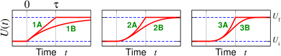
Figure 1: Ramp shapes. We illustrate $U_{\rm f}>U_{\rm i}$; it should be straightforward to visualize $U_{\rm f}<U_{\rm i}$ cases. Each [A], [B] pair has the same initial behavior — linear, quadratic and cubic for the three pairs. The [B] versions have no endpoint kinks.

III Ramp shapes

We analyze interaction ramps of the form

$$U(t)~{}=~{}U_{\rm i}~{}+~{}\theta(t)\,(U_{\rm f}-U_{\rm i})\,s(t/\tau)\,.$$

The ramp function $s(x)$ starts at $s(0)=0$ and ends at $s(\infty)=1$. The ramps take place over time scale $\tau$ but we do not require them to end at $t=\tau$. (Contrast, e.g., Ref. EcksteinKollar_NJP2010 .) We choose a collection of ramps which allows us to compare the presence/absence of kinks and various exponents.

Specifically, we consider the following forms for $s(x)$:

$${\rm[1A]}\quad x\;\theta(1-x)+\theta(x-1) {\rm[1B]}\quad 1-e^{-x}$$

$${\rm[2A]}\quad x^{2}\;\theta(1-x)+\theta(x-1) {\rm[2B]}\quad 1-e^{-x^{2}}$$

$${\rm[3A]}\quad x^{3}\;\theta(1-x)+\theta(x-1) {\rm[3B]}\quad 1-e^{-x^{3}}$$

Each [A], [B] pair has the same initial behavior, $s(x){\sim}x^{\alpha}$, but the [B] versions have no endpoint kinks (Fig. 1).

Figure 2: The normalized excitation energy or heat, $Q(\tau)/Q(0)$, for various trapped systems. ($U_{\rm i}$,$U_{\rm f}$) values and trap constants $k_{\rm tr}$ are chosen over a wide range to emphasize the parameter-independence of the effects. Response to [A] ramps (left panels) shows overall $Q(\tau)\sim\tau^{-2}$ decay, with superposed oscillations that decay faster for larger-$\alpha$ ramps. For [B] ramps (right panels) the asymptotic behavior is pure $\tau^{-2\alpha}$ decay. Insets to (c): density profiles for $U=U_{\rm i,f}$ ground states. For (f), $U=U_{\rm i,f}$ ground-state profiles are very similar, only $U_{\rm i}$ shown.

IV Universal features of ramp response

In Fig. 2 we present the behavior of the heat function $Q(\tau)$, normalized against its instantaneous-quench value $Q(\tau=0)$. The small-$\tau$ behavior and the exact magnitude of $Q(\tau)$ are system- and approximation-dependent; the universal features we present concern only the large-$\tau$ asymptotics of $Q(\tau)/Q(0)$.

In the left panels, the $Q(\tau)$ behaviors are compared for the ramp shapes $s(x){\sim}x^{\alpha}$ with discontinuous derivatives at endpoints, [1A], [2A], [3A]. Each curve has an overall power-law decay with the same decay exponent, $Q(\tau)\sim\tau^{-2}$. This suggests that the residual energy for such ramps is primarily set by the endpoint kink. Superposed on the power-law decay are oscillations, which are often but not always smaller for larger $\alpha$ (contrast panels (c) with others). The oscillation strength decays faster for larger $\alpha$, as $\sim\tau^{-(\alpha+1)}$.

The right panels concern smoothed ramps [1B], [2B], [3B], which lead to non-oscillating decay of $Q(\tau)$. The decay exponent is seen to depend on the power $\alpha$ of $s(x)\sim{x^{\alpha}}$, namely, $Q(\tau)\sim\tau^{-2\alpha}$.

The dimensionality does not affect the decay exponents or general behavior. As an example, results are shown for the BEC in 1D, 2D, and 3D, in the (d) panels and insets. We have also found that the same exponents and oscillation features also appear in additional cases not shown, e.g., a continuum Fermi superfluid (3D, $U<0$), the Bose-Hubbard model in higher $D$ (treated via the Gutzwiller approximation), etc.

The (c) and (f) panels involve systems which cannot be described as having single-radius profiles. The two spin components have different extents in the spin-imbalanced Hubbard model (c); the Bose-Hubbard situation (f) has superfluid wings around a Mott core. The $Q(\tau)$ behaviors are more rich for these systems; however, the features discussed above remarkably also persist in these more complex cases.

V Radius dynamics interpretation

We now show how radius dynamics explains the $Q(\tau)$ behaviors presented above. We will use the convenient formulation of BEC radius dynamics, Eqs. (1) and (2). Fig. 3 (top row) shows the radius of a 2D BEC evolving as a function of time for various ramp shapes, for reasonably large $\tau$. In the center and bottom rows, we show the deviation of $\sigma(t)$ from the equilibrium radius corresponding to the instantaneous value of the interaction, $R_{0}(t)=R_{0}[U(t)]$. For a truly adiabatic ramp, $\sigma(t)$ would follow $R_{0}(t)$ exactly; therefore the deviation $f(t)=\sigma(t)-R_{0}(t)$ is at the heart of non-adiabaticity and this quantity determines the heating $Q$. After the ramp, the $f(t)$ function is purely oscillatory; $Q$ scales as the square of the oscillation magnitude. The oscillations initiated at the beginning of the ramp are of magnitude $\mathcal{O}(\tau^{-\alpha})$ for the $(t/\tau)^{\alpha}$ ramp. In the case of [A] ramps (middle row), the endpoint kink causes an $\mathcal{O}(\tau^{-1})$ oscillation, which is parametrically larger for $\alpha>1$ and hence dominates the final dynamics, leading to overall $Q(\tau)\sim\tau^{-2}$ behavior.

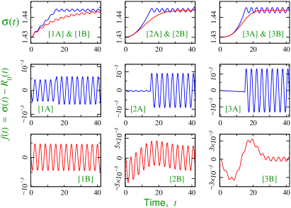
Figure 3: Top row: radius dynamics $\sigma(t)$ for various ramp shapes, $\tau=15$. Center and bottom rows: deviation $f(t)$ from the ‘instantaneous’ ground-state radius $R_{0}(t)$. 2D BEC; ($U_{\rm i}$,$U_{\rm f}$) = (20,21).

[A] ramp shapes.

We first explain the $\sim\tau^{-1}$ scaling of oscillations initiated at the kink. If we neglect the smaller oscillations at $t<\tau$, the radius $\sigma(t){\approx}R_{0}(t)$ at the kink $t=\tau$ has “correct” value for $U=U_{\rm f}$, i.e. $f$ is negligible. However the derivative is nonzero, $\sigma^{\prime}(t){\approx}R_{0}^{\prime}(t)|_{t=\tau}$, which scales as $\sim\tau^{-1}$. Thus we have the following “initial” conditions at $t=\tau^{+}$ for subsequent evolution: $f(\tau)=0$, $f^{\prime}(\tau^{+})=c_{0}\tau^{-1}$. Using $f(t>\tau)\approx\rho\sin(\Omega_{B}{t}+\delta)$, these initial values imply $\rho\sim\tau^{-1}$. This explains the $\mathcal{O}(\tau^{-1})$ oscillation magnitude of $f(t>\tau)$, and hence $\mathcal{O}(\tau^{-2})$ heating, for ramps having an endpoint kink.

The oscillations of $Q(\tau)$ (Fig. 2 left panels) can be explained by relaxing the approximation $f(t<\tau)\approx 0$ made above. The small oscillations of $f(t<\tau)$ guarantee that $\sigma^{\prime}(t=\tau)$ oscillates around $R_{0}^{\prime}(t=\tau)$ as a function of $\tau$. This causes the final breathing mode amplitude $\rho$ to oscillate around its $\mathcal{O}(\tau^{-1})$ value as a function of $\tau$. The $f(t<\tau)$ oscillation strength is $\mathcal{O}(\tau^{-\alpha}$) (shown below). As a result, if $f(t>\tau)\approx\rho\sin(\Omega_{B}{t}+\delta)$, we will have

$$\rho~{}\sim~{}\frac{c_{1}}{\tau}+\frac{c_{2}T(\tau)}{\tau^{\alpha}}$$

where $T(x)$ is an oscillatory function. Therefore, the excess energy ($\sim\rho^{2}$) has an $\mathcal{O}(\tau^{-\alpha-1})$ oscillatory correction to the leading $\mathcal{O}(\tau^{-2})$ decay. The oscillations in $Q(\tau)$ therefore decay as $\tau^{-(\alpha+1)}$, as seen in Fig. 2 left panels.

Smoothed [B] ramp shapes.

For smooth [B] ramps (Fig. 3 bottom), the breathing-mode strength ($\sim\tau^{-\alpha}$) initiated at the beginning of the ramp remains unchanged; there is no kink to abruptly create larger oscillations. We therefore need only to explain the strength of oscillations at the beginning of the ramp, where $s(t/\tau)\approx(t/\tau)^{\alpha}$. For this, we rewrite Eq. (1) as an equation for $f(t)$. For simplicity, we will write this out explicitly only in the limit $U_{\rm i,f}\gg 1$, and small oscillations, $f(t){\ll}R_{0}(t)$. (The arguments can of course be modified to go beyond the large-$U$ restriction. Small $f(t)$ is guaranteed for large $\tau$.) We obtain

$$f^{\prime\prime}(t)+\Omega_{B}^{2}f(t)+\frac{u^{\prime\prime}(t)}{(D+2)u^{\frac{D+1}{D+2}}}-\frac{(D+1)u^{\prime}(t)^{2}}{(D+2)^{2}u^{\frac{2D+3}{D+2}}}=0,$$ (4)

with $u=U/(2\pi)^{D/2}$. The first two terms give pure oscillations, i.e., breathing mode at fixed $u$ with frequency $\Omega_{B}\approx\sqrt{D+2}\omega_{\mathrm{tr}}$. The last two terms are corrections due to time-varying interaction. We first treat $\alpha>1$ ramps. The initial conditions at $t=0^{+}$ are then $f(0)=f^{\prime}(0)=0$. With $u=u_{i}+(\delta{u})(t/\tau)^{\alpha}$, the $u^{\prime\prime}$ correction is dominant compared to the $u^{\prime 2}$ correction at $t\ll\tau$. The dominant correction terms take the form $c_{1}/\tau^{2}$ for $\alpha=2$, and $c_{1}t/\tau^{3}$ for $\alpha=3$. The solutions of the resulting differential equation are sums of oscillatory and algebraic terms. It is straightforward to verify that the boundary conditions $f(0)=f^{\prime}(0)=0$ force the oscillatory part to have coefficients scaling as $\sim\tau^{-\alpha}$. This explains the $Q\sim\tau^{-2\alpha}$ behavior for integer $\alpha>1$. The $\alpha=1$ case is slightly different. The initial condition still involves $\sigma^{\prime}(0)=0$, but since $R_{0}(t)=[u(t)]^{1/(D+1)}$ has finite slope at $t=0^{+}$, this now corresponds to $f^{\prime}(0^{+})=-R_{0}^{\prime}(0^{+})=-c_{3}/\tau$. This initial condition leads to a purely oscillatory $f(t)$ with amplitude $\sim\tau^{-1}$, which explains $Q(\tau)\sim\tau^{-2}$ for $\alpha=1$.

VI Spectral Interpretation

For small changes of interaction, one can use the elegant perturbative results of Ref. EcksteinKollar_NJP2010 to interpret our generic results in terms of the spectal structure of many-body systems in harmonic traps. The perturbative expression is

$$Q(\tau)\propto\int\frac{d\omega}{\omega}\Gamma(\omega)F(\omega\tau)$$ (5)

where

$$F(u)~{}=~{}\left|\int_{0}^{x_{\rm max}}dxs^{\prime}(x)e^{iux}\right|^{2}$$ (6)

encodes the relevant information about the rampshape $s(x)$ ($x_{\rm max}$ is 1 for [A] ramps and $\infty$ for [B] ramps), and

$$\Gamma(\omega)~{}\propto~{}\sum_{n\neq 0}\left|\langle\left.{\phi_{n}}\right|\hat{W}\left|{\phi_{0}}\right.\rangle\right|^{2}\delta(\omega-\epsilon_{n0})$$ (7)

encodes the relevant spectral structure of the system EcksteinKollar_NJP2010 . Here $\left|{\phi_{n}}\right.\rangle$’s are the eigenstates of the system, $\epsilon_{n0}$ are the eigenenergies measured from the ground state energy, and $\hat{W}$ is the perturbing operator, i.e. the part of the Hamiltonian being ramped, in our case the interaction term.

The eigenspectra of interacting systems in harmonic traps are not known in great detail, to the best of our knowledge. However, we can make the following general observations. The lowest excited eigenstates (at or around $\omega_{\rm tr}$) are spatially asymmetric, and are therefore not excited by interaction ramps, due to symmetry. (Excitation of these eigenstates would lead to dipole mode oscillations of the cloud center of mass.) The states at or around $2\omega_{\mathrm{tr}}$ are more relevant for interaction ramps. Since these spatially-symmetric eigenstates have radial size larger than the ground state, a small component of these eigenstates in the wavefunction leads to breathing-mode oscillations. Since the interaction affects the ground-state radial size of the trapped system, at least one of these states around $2\omega_{\mathrm{tr}}$ should be excited in an interaction ramp. The excitation energy of this eigenstate over the ground state is the breathing mode frequency $\Omega_{B}$.

(Above, we conjectured the lowest antisymmetric and lowest symmetric excited states to lie around $\omega_{\mathrm{tr}}$ and around $2\omega_{\mathrm{tr}}$ respectively, because that is the spectral structure of the non-interacting gas. With interactions, it may be reasonable to presume a similar structure. Our argument below does not depend on the exact values of the excitation energies.)

Since we are interested in large $\tau$ and are now considering the perturbative situation, we will approximate the lowest spatially symmetric eigenstate to be the only excitation. i.e., $\Gamma(\omega)\propto\delta(\omega-\Omega_{B})$. With this approximation, the heat function is simply

$$Q(\tau)\propto F(\Omega_{B}\tau)\ ,$$ (8)

i.e., it is completely set by the ramp shape except for the breathing mode frequency $\Omega_{B}$ setting the scale for $\tau$.

Evaluating $F(u)$ for the different rampshapes, we find the following expressions for the normalized excitation energy $Q(\tau)/Q(0)$:

$${\rm[1A]}\qquad\frac{4\sin^{2}(\tilde{\tau}/2)}{\tilde{\tau}^{2}}$$

$${\rm[2A]}\qquad\frac{4}{\tilde{\tau}^{2}}-\frac{8\sin\tilde{\tau}}{\tilde{\tau}^{3}}+\frac{16\sin^{2}(\tilde{\tau}/2)}{\tilde{\tau}^{4}}$$

$${\rm[3A]}\qquad\frac{9}{\tilde{\tau}^{2}}+\frac{36\cos\tilde{\tau}}{\tilde{\tau}^{4}}-\frac{72\sin\tilde{\tau}}{\tilde{\tau}^{5}}+\frac{146\sin^{2}(\tilde{\tau}/2)}{\tilde{\tau}^{6}}$$

$${\rm[1B]}\qquad\frac{1}{1+\tilde{\tau}^{2}}$$

with $\tilde{\tau}\equiv\Omega_{B}\tau$. The [2B] and [3B] cases can be written in terms of special functions; it is not helpful to write out these complicated expressions in full, but they have the correct asymptotics, $\sim\tilde{\tau}^{-4}$ ([2B]) and $\sim\tilde{\tau}^{-6}$ ([3B]). Figure 4 plots these results. Clearly, all the features presented in Sec. IV and Figure 2 are reproduced from this simplified analysis. The sole exeption is that the [1A] case would requre a non-oscillating $\tau^{-2}$ term to match the forms found for the physical systems. This can presumably be obtained by going beyond perturbation theory.

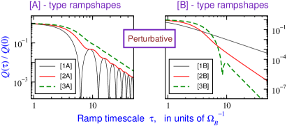
Figure 4: Excess energy predictions from perturbative formalism EcksteinKollar_NJP2010 based on spectral considerations (Sec. VI in text).

VII Discussion; Open questions

VII.1 Summary and context

Considering various harmonic-trapped atomic clouds, we have presented results on the adiabaticity question, demonstrating system-independent aspects in the first corrections to adiabatic behavior for slow ramps. We have shown that the slow-ramp response is determined by the radius-oscillation modes common to many trapped atomic systems, and its exact form depends on the ramp shape. We have explained the universal effects using a single-radius description of the cloud. This covers a wide range of interesting systems, but it is even more remarkable that our universal features extend to at least some systems which cannot be described by a single radius. In the perturbative regime (small quenches), the generic features can be alternatively derived by using the formalism of Ref. EcksteinKollar_NJP2010 , assuming a single excited eigenstate to determine the heating. The connection between the two pictures is that the excited eigenstate is expected to be (one of) the lowest spatially-symmetric eigenstates which has different size compared to the ground state; hence excitation of this eigenstate leads to breathing-mode oscillations of the cloud size.

We have shown that a final kink in the ramp shape plays a drastic role in the non-adiabatic response of compressible trapped systems. A recently discovered effect of such kinks is logarithmic contributions to $Q(\tau)$ Polovnikov_AdiabaticPertThy ; EcksteinKollar_NJP2010 ; DoraHaqueZarand_arxiv10 . The effect we have found for trapped systems (kink induces larger oscillations overwhelming initial excitation) is quite different.

VII.2 Open questions

Our work opens up several new research avenues. Like other “universal” results, it is important to identify the limits of validity. For example, do the same $Q(\tau)$ asymptotic features appear in trapped systems not described by a single radius? Paradigm examples are Bose-Hubbard systems containing superfluid-insulator “wedding-cake” structures, and phase-separated imbalanced Fermi gases near unitarity. We have shown some examples where the same behaviors appear [Figs. 2(c,f)], but a general understanding is lacking. It is likely that the dynamics of one radius-like variable generally dominates the extreme asymptotics, recovering our results.

Each of the systems are of intense interest in their own right, and understanding less universal features in parameter quenches is important for the individual systems, especially with growing experimental interest and capabilities for studying ramps and quenches. Ramps in the trapping frequency should also induce radius oscillations, but details might be different from interaction ramps. The case of anisotropic harmonic traps also remains an open issue. One might speculate that one of the trapping frequencies dominate the extreme asymptotics, but the intermediate-$\tau$ region might show interesting interplay of the several frequencies and associated radii. Physical insights developed in our study of $Q(\tau)$ can perhaps be applied to better understand “optimal ramp” studies seeking to find ramp paths producing minimal heating Muga_delCampo_frictionless . Finally, the spectral considerations of Sec. VI highlight that the spectral structure of many-body systems in the presence of an external harmonic trap deserves to be better studied.

Appendix A Calculation Methods and Approximations

In this appendix we provide details on the methods and approximations used to obtain the $Q(\tau)$ results that are presented in Figure 2 for the different model systems.

A.1 Lattice systems

For the data of Fig. 2(a-c) (fermionic and bosonic Hubbard models), we time-evolved the full wavefunctions numerically exactly. The initial wavefunction was obtained by Lanczos diagonalization of the Hamiltonian with initial interaction $U_{\rm i}$. For ramps (changing Hamiltonian), numerical time evolution of the full wavefunction is more challenging than time-evolving under a constant Hamiltonian, for which efficient Krylov subspace based methods exist evolution_Krylov . One option for ramps is to break the evolution into time-steps within which the Hamiltonian is approximated to be constant. Instead, we used Runge-Kutta evolution with adaptive stepsize. Calculating $Q(\tau)$ at large $\tau$ (where $Q$ becomes small) requires high precision as $Q(\tau)$ is a difference between two energies that are close in value. Because of these restrictions, the Hilbert spaces for the data shown in Fig. 2(a-c) were around ${\sim}10^{5}$. Typically we used five to ten bosons or fermions in ten to fifteen sites. Relatively strong traps, $k_{\rm tr}\sim\mathcal{O}(1)$, were used in order to ensure that the cloud edges did not reach the lattice edges.

For the Bose-Hubbard model, the exact evolution was complemented by calculations using the Gutzwiller approximation, e.g., Fig. 2(f), which allows for larger sizes. This is a widely used approach for time evolution in Bose-Hubbard systems; see. e.g., Ref. Lewenstein_review for a recent description. The ansatz wavefunction is

$$\left|{G(t)}\right.\rangle~{}=~{}\prod_{i}\sum_{n}f_{n}^{(i)}(t)\left|{n;i}\right.\rangle$$ (9)

where $\left|{n;i}\right.\rangle$ is the $n$-boson Fock state on site $i$. The $f_{n}^{(i)}$ parameters for a particular site $i$ may be regarded as the components of a local wavefunction, which evolve according to the local site Hamiltonian

$$\hat{H}_{i}~{}=~{}(V_{i}-\mu)n_{i}+{\tfrac{1}{2}}Un_{i}(n_{i}-1)\\ -{b}_{i}\sum_{<j>}\Phi_{j}^{*}-{b}_{i}^{\dagger}\sum_{<j>}\Phi_{j},$$ (10)

where $V_{i}={\tfrac{1}{2}}k_{\rm tr}i^{2}$ is the trap potential, the $j$ index runs over all sites neighboring the $i$ site, and

$$\Phi_{j}~{}=~{}\langle{b_{j}}\rangle~{}=~{}\sum_{n}\sqrt{n+1}\,f_{n}^{(j)*}f_{n+1}^{(j)}$$

is the condensate fraction at site $j$. As in the case of full wavefunction evolution, Gutzwiller evolution is much more demanding for a changing Hamiltonian compared to evolution under a constant Hamiltonian, even more so in our case because of the high precision required for the final energy in order to calculate $Q(\tau)$. We employed imaginary time evolution to find the initial ground state, and then Runge-Kutta (with adaptive timestep size) to evolve the coupled equations for $f_{n}^{{i}}(t)$ in real time with changing $U(t)$.

A.2 Continuum systems

Bose condensate.

In addition to numerical solutions of the GP equation, we have also used a single-parameter variational description to describe the dynamics, using the condensate size $\sigma(t)$ as the time-dependent parameter. This description is particularly convenient for analyzing breathing-mode dynamics, as we have done in Section V.

The radius description is formulated in terms of a Gaussian variational ansatz, which for 1D is

$$\psi(x,t)=\frac{1}{[\sqrt{\pi}\sigma(t)]^{1/2}}\exp\left[-\frac{x^{2}}{2[\sigma(t)]^{2}}-i\beta(t)x^{2}\right].$$ (11)

For $D>1$ the variational wave function is a product of one such Gaussian factor for each dimension. Using this ansatz in the GP Lagrangian

$$L=\frac{i}{2}\int_{r}\left(\psi^{*}\frac{\partial\psi}{\partial{t}}-\psi\frac{\partial\psi^{*}}{\partial{t}}\right)-E[\psi]\ ,$$ (12)

the Euler-Lagrange equations of motion give the evolution equations for the variational parameters $\sigma(t)$ and $\beta(t)$. This is a standard and widely-used technique for GP dynamics, dating back to Ref. PerezGarcia_Cirac_Lewenstein_Zoller_variational .

The imaginary part in the wave function (11) is necessary because time evolution from a real wave function produces an imaginary component. However, the two parameters turn out to be not independent but simply related ($\beta(t)\propto\partial_{t}\ln\sigma(t)$). There is thus effectively a single dynamical parameter describing the system, namely the cloud radius $\sigma(t)$. The resulting equation of motion for $\sigma$ is found to be Eq. (1), and the energy in terms of $\sigma$ is given by Eq. (2).

In comparing the single-parameter variational description with the full GP equations,, we find that the normaized excess energy, $Q(\tau)/Q(0)$, is reproduced almost exactly by the single-parameter description, but that the $Q(\tau)$ values obtained from Eqs. (1), (2) do not have the correct normalization and deviate by a factor from full-GP results. Note that the normalization does not affect any of the universal behaviors (Sec. IV, Fig. 2) under discussion in this Article.

We could just as well use a Thomas-Fermi instead of Gaussian profile. The results are very similar and do not substantially affect any of the arguments we make in this work. The equation of motion in that case loses the $\sigma^{-2}$ term of Eq. (1) (Sec. II).

Continuum two-component Fermi system.

To perform non-equilibrium calculations for two-component (spin-$\tfrac{1}{2}$) continuum fermionic gases, we have used a quantum hydrodynamic approximation. The formulation of Refs. fermions_tddft in terms of a nonlinear Schrödinger equation (“time-dependent DFT”) is convenient for our purposes because of its slimiarity to the GP description of continuum bosons.

The time-dependent DFT formulation has been used successfully for the unitary Fermi gas (reviewed in Ref. Bulgac_1301_review ). We do not consider the unitary limit in this work because the interaction is fixed at infinity and thus cannot be ramped as a time-dependent parameter. We focus on weakly interacting gases so that we can use the relatively simple Hartree approximation and the interaction $U(t)$ appears explicitly and can be ramped. In this work we have restricted ourselves to 3D and to equal populations of the two components.

Using the Hartree approximation for the chemical potential (main text Eq. (3)), the hydrodynamic equation becomes

$$i\hbar\partial_{t}\psi=\left[-\frac{\hbar^{2}}{2m}\nabla^{2}\psi+V_{\rm ext}+\frac{U(t)}{2}|\psi|^{2}+\alpha|\psi|^{4/3}\right]\psi$$ (13)

with $\alpha=\tfrac{1}{2}\left(3\pi^{2}\right)^{2/3}$, and $n=|\psi|^{2}$ here is the total density of the two spin states. Note the interaction being ${\tfrac{1}{2}}Un$ rather than $Un$. Each fermion interacts with half of all the fermions, those with the opposite spin.

In contrast to the Bose condensate case, it is not consistent to normalize $\psi$ to unity. This means that there are no factors of $N$ absorbed in the definition of $U$ in the continuum fermionic system, as opposed to the continuum Bose condensate. This difference is responsible for the rather different ranges of values for the $U(t)$ of BECs in Figure 2(d) and the $U(t)$ of the 3D Fermi gas in Figure 2(e).

As in the Bose condensate case, we employ the variational ansatz

$$\psi({\bf r},t)~{}=~{}\frac{\sqrt{N}}{\sqrt{\pi^{3/2}\sigma^{3}}}\exp\left[\frac{1}{2}\left(\frac{r}{\sigma}\right)^{2}-i\beta r^{2}\right].$$ (14)

Note the factor $\sqrt{N}$. The contrast to Eq. (11) is due to the different normalization. The Euler-Lagrange equations provide equations of motion for $\sigma(t)$ and $\beta(t)$. The two parameters are not independent ($\beta=-\frac{1}{2}\frac{\dot{\sigma}}{\sigma}$, identical to the GP case). Eliminating $\beta$, we get a single-parameter description. The equation of motion for $\sigma$ is

$$\sigma\ddot{\sigma}+\sigma^{2}-\frac{1}{\sigma^{2}}-\frac{UN}{2(\sqrt{2\pi}\sigma)^{3}}-\tfrac{4}{3}\left(\tfrac{3}{5}\right)^{5/2}\frac{N^{2/3}\alpha}{\pi\sigma^{2}}=0\ ,$$ (15)

and the energy equation is

$$E=\frac{3N}{4}\left[\frac{1}{\sigma^{2}}+\dot{\sigma}^{2}+\sigma^{2}\right]+\frac{1}{(2\pi)^{3/2}}\frac{UN^{2}}{4\sigma^{3}}+\left(\tfrac{3}{5}\right)^{5/2}\frac{N^{5/3}\alpha}{\pi\sigma^{2}}.$$ (16)