Phurbas: An Adaptive, Lagrangian, Meshless, Magnetohydrodynamics Code. II. Implementation and Tests

Abstract

We present an algorithm for simulating the equations of ideal magnetohydrodynamics and other systems of differential equations on an unstructured set of points represented by sample particles. The particles move with the fluid, so the time step is not limited by the Eulerian Courant-Friedrichs-Lewy condition. Full spatial adaptivity is required to ensure the particles fill the computational volume, and gives the algorithm substantial flexibility and power. A target resolution is specified for each point in space, with particles being added and deleted as needed to meet this target. We have parallelized the code by adapting the framework provided by GADGET-2. A set of standard test problems, including $10^{-6}$ amplitude linear MHD waves, magnetized shock tubes, and Kelvin-Helmholtz instabilities is presented. Finally we demonstrate good agreement with analytic predictions of linear growth rates for magnetorotational instability in a cylindrical geometry. This paper documents the Phurbas algorithm as implemented in Phurbas version 1.1.

1. Introduction

In Maron et al. (2012, hereafter Paper I) we described an adaptive, Lagrangian, meshless, method for magnetohydrodynamics (MHD). We now describe the parallel implementation of this algorithm and its tests, and discuss its practical properties. The test problems used are selected from the accepted ones in the literature; many follow those documented for Athena (Stone et al., 2008), and those used by Tóth (2000), and Ryu & Jones (1995). The three goals of the tests are to verify the convergence to smooth solutions of the MHD equations, demonstrate the global conservation properties and shock errors, and finally to verify the ability of Phurbas to model the linear growth of magnetorotational instability correctly.

In § 2.1 we describe how we have implemented our algorithm into a parallel code called Phurbas using the GADGET-2 code (Springel, 2005) as a basis. We describe the tests that we have performed with this implementation in § 3. We summarize the results of the tests, and discuss the implications and future prospects for Phurbas-like methods in § 4.

2. Implementation of the Algorithm

Phurbas is a parallel code using the Message Passing Interface, following the patterns of the GADGET-2 code (Springel, 2005), which originally combined a smoothed particle hydrodynamics (SPH) treatment of gas dynamics with a tree solution of the Poisson equation to follow N-body dynamics. The serial particle update module described in Paper I has been incorporated into a modified version of GADGET-2 that has been re-purposed to serve as a parallel framework. We refer to the version documented in this work as Phurbas version 1.1 to allow for the differentiation of future modifications to the algorithm and the code. (We note that tests of Phurbas 1.0 were described in the first submitted version of this paper, posted to ArXiv as version 1 of this paper.)

We summarize here the algorithm described in detail in Paper I. Phurbas solves the equations of ideal MHD, expressed in terms of Lagrangian time derivatives. The equations are discretized on an adaptive set of particles that carry values of the field variables (density $\rho$, velocity V, magnetic field B, and internal energy density $\sigma$). The particles move with the velocity V that they carry, making the Lagrangian formalism the natural description of the time evolution of the field variables. The evolution equations relate time derivatives of the field variables to their spatial derivatives. To calculate the spatial derivatives, Phurbas uses a local, third-order, polynomial, moving least squares interpolation, using neighbor particle values drawn from a sphere of radius $r_{f,i}=2.3\lambda_{i}$ about particle $i$, where $\lambda_{i}$ is the effective resolution parameter. A second order predictor-corrector scheme is used with the time derivatives obtained by applying the MHD equations to the approximate spatial derivatives to advance the particle positions and variable values.

Particles are added and deleted, filling voids and destroying clumps, to ensure that each sphere of radius $r_{f}$ is well sampled. On average, the particle creation and deletion results in at least one particle per volume $\lambda^{3}$. The resolution parameter $\lambda$ need not be constant in space or time, and each particle has an individual time step. In this sense Phurbas is fully adaptive both spatially and temporally. The time steps are independent of the bulk velocity of the flow. Spatial variation of the time steps is limited to prevent the penetration of short time step particles into regions of long time step particles.

To obtain numerical stability, Phurbas integrates a modified version of the ideal MHD equations including a bulk viscosity. The bulk viscosity coefficient is broken into two scalar fields. The first is scaled so that motions near the grid scale are always damped. The second adapts to provide damping in regions with large change, such as shocks and contact discontinuities. A diffusive correction term in the induction equation locally diffuses nonzero ${\nabla\!\cdot\!\textbf{\em B}}$ away.

2.1. GADGET-2 Based Implementation

In this section we outline the changes made to GADGET-2 to adapt it to Phurbas, which serves also to highlight the differences in the infrastructure needed to support SPH and Phurbas. The largest modifications are the removal of the SPH algorithm for evaluating the spatial derivatives, the addition of data passing and elements in the data structures needed for the Phurbas MHD algorithm, the modification to support addition and deletion of gas-type particles, the addition of magnetic field variables, and a new main time advance loop. Additions to the input-output routines and global statistics were also made.

In GADGET-2 SPH, the sums required for value and gradient evaluation are computed in a distributed manner. The contribution to each sum from a set of neighbor particles can be computed on the processor where those neighbors reside, so that only the total value need be communicated. For the Phurbas particle update, the values for all particles within $r_{f,i}$ of particle $i$ must be communicated to the process hosting particle $i$. Particles are updated in batches, so within groups of $\sim 5,000$–10,000 particles duplicate neighbor communications can be avoided.

Phurbas requires only a strict radius-based neighbor search, unlike in GADGET-2 SPH where a mutual neighbor relation is required to achieve symmetric interparticle forces. The Phurbas neighbor search is also performed on a fixed radius volume, so it does not need iterative refinement like the GADGET-2 SPH neighbor search, which adapts the neighbor search radius to include a target number of neighbors. In Phurbas, the moving least squares interpolation and the particle adaption algorithm require information from the neighbor particles of particle $i$ to be retrieved to the host process of particle $i$. The set of particles used for these three procedures is the same, the particles within $r_{f}$.

Compared to GADGET-2 SPH particles, Phurbas particles use somewhat more memory. Phurbas uses 56.5 eight byte variables per particle as opposed to the 36.5 used by GADGET-2 in double precision mode. We retain the basic structures of GADGET-2 in that the variables required for the neighbor tree construction are stored in a separate array from the fluid quantities. As the memory required to complete the retrieval of neighbor information can be much larger than in GADGET-2 SPH, and dynamically varies, we dynamically allocate buffers as needed to complete this step and free the memory after the process is finished. Compared to GADGET-2 SPH, we have modified the code to avoid persistent allocation of memory, which in particular alleviates problems with computing the domain decomposition with large numbers of parallel processes.

The void search in Phurbas described in Paper I relies on computing distances to neighbor particles placed on a $9^{3}$ grid. This procedure gains in computational speed if the three-dimensional grid is implemented as a one-dimensional list in memory that is shortened each time a grid point is eliminated from consideration as a nearest neighbor. This minimizes the number of times each grid point must be accessed, while keeping the values arranged compactly in memory. We have implemented this strategy by simply replacing the coordinates of any eliminated point with the coordinates of the current last point on the list and shortening the length of the list.

GADGET-2 does not support dynamic particle addition and deletion. In Phurbas, we first perform a load balance on the list of particles to add to voids, in order to distribute them among processes evenly. The particles are created in free memory spaces on the processors where they are moved to by the load balance algorithm. Particles in clumps are deleted from the processors they are resident on.

As we have now deleted some particles, and added others to essentially random processors, we perform a new global GADGET-2 load balance calculation, followed by a Peano-Hilbert ordering and tree build, as in the standard GADGET-2 algorithm (Springel, 2005). Doing this on the entire particle list brings the new particles to optimal positions on the processors and provides neighbor information for the subsequent processing stages.

The restriction of local time step variations only requires information from particle $i$ to be sent to the host processes of the neighbors of particle $i$.Time steps are rounded down to powers of two in order to use the GADGET-2 binary block time step scheme (Springel, 2005), and the increase in time step is limited with the GADGET-2 synchronized time step scheme.

The most significant optimization made has been for the assembly of the left hand side matrix for the least squares fitting problem used in the polynomial interpolation. This has been explicitly loop-unrolled into very simple FORTRAN designed to maximize the ability of the compiler to pipeline the instructions and optimize cache use. Despite the increased memory use compared to GADGET-2 SPH, our experience has been that simulations are computation limited rather than memory limited.

Compared to dark matter dominated, cosmological, N-body problems, pure MHD fluid problems intrinsically require more work per particle per time step. For the highest resolution run in the cylindrical geometry MRI test in the following section, we used $\sim 10^{6}$ particles on 48 cores, 95% of which were typically active, non-boundary particles. This was run on the Texas Advanced Computation Center Lonestar cluster, which consists of nodes with dual Xeon Intel, hexacore, 3.33 GHz, 64-bit, Westmere processors (13.3 GFLOPS per core) interconnected with InfiniBand QDR. Phurbas took an average $\sim 1.3\times 10^{-4}$ seconds for the serial procedures per particle (void and clump checks, moving least squares interpolations, time derivative calculations, and time integration corrector step). We note that the performance of this section of the code depends highly on the compiler and optimization settings used. The wallclock time per step was $\sim 5$ seconds for a step involving $\sim 9.1\times 10^{5}$ active particles, giving a speed of $\sim 2.6\times 10^{-4}$ seconds per particle or $3.8\times 10^{3}$ total updates per core per wallclock second, including adaptivity involving $\sim 1500$ additions and deletions. It should be noted that Phurbas version 1.1 code has not yet been heavily optimized, so we believe the parallel overhead can be further reduced.

For a given application to be suitable for simulation with Phurbas, the Lagrangian nature, adaptivity, and individual time steps of Phurbas must offer a significant advantage on a problem. Otherwise a high-order, grid-based method such as the Pencil Code (Brandenburg & Dobler, 2002) is a more efficient choice, as it computes more than $10^{2}$ times more updates per core per second.

3. Tests

We present in this section a series of tests that serve to verify the performance of Phurbas, and illustrate its abilities and limitations. These include linear waves (Sec. 3.1), circularly polarized Alfvén waves (Sec. 3.2), hydrodynamical and MHD shock tubes (Sec. 3.3), Kelvin-Helmholtz instabilities (Sec. 3.4), and cylindrical magnetorotational instability (Sec. 3.5).

As Phurbas is meshless, it is an intrinsically three-dimensional algorithm. The performance and design criteria are different in different numbers of dimensions. Hence, even when tests have symmetries such that they could be stated in a lower number of dimensions, we perform them in fully three-dimensional domains to achieve results reflective of the true capabilities of the code.

It is important to use realistic particle distributions for these tests. Though perfectly gridded particle distributions would yield good results for some tests, as has been demonstrated in the literature, such well arranged distributions cannot be expected in a general flow. Instead, we realize cubes of relaxed, glassy particle distributions using several iterations of Phurbas’s void and clump detection algorithms, and then tile these distributions to fill the problem domain. This also ensures that initially, no particle adaption occurs until the particles move far enough to justify it. This allows both the use of a realistic particle distribution and makes it possible to create a set of predictably refined initial conditions for convergence studies. Irregular initial particle distributions also remove the need to set up tests at odd angles to prevent aligning waves and shock fronts with a grid.

3.1. Linear Waves

Figure 1.— Convergence of linear waves. Points show the relative $L_{1}$-norm errors derived from the comparison of Phurbas results to solutions of the MHD dispersion relation including the stabilizing bulk viscosity (see Appendix A). The slopes plotted show second-order convergence.

To verify the convergence of the scheme and its accuracy in the linear domain, three MHD waves are modeled. The three waves are a magnetoacoustic wave propagating perpendicularly to the background magnetic field, a shear Alfvén wave propagating along the background field, and a sound wave propagating in an unmagnetized medium. We compare the results with solutions of the dispersion relation for the MHD equation, including the bulk viscosity $\zeta_{l}$. The solutions for the magnetoacoustic and sound waves are derived in Appendix A.

To set this problem up, we use a cubic domain, with side length 1.0, is initialized with density $\rho=1$, pressure $P=1/\gamma$, and adiabatic index $\gamma=5/3$, in which the waves propagate in the $x$-direction. For the magnetoacoustic wave the magnetic field is $\mathbf{B}=\sqrt{3}\hat{\mathbf{z}}$, for the Alfvén wave it is $\mathbf{B}=1.0\hat{\mathbf{x}}$, and for the sound wave the magnetic field is set to zero. The initial condition is generated from a relaxed particle distribution so that no particle deletion or addition initially occur. For runs with resolution higher than the lowest value, the same set of particles used in the lowest resolution test is scaled and tiled to fill the computational volume. The wave is propagated one wavelength, and then the $L_{1}$-norm error is summed across all fields. We analyze the convergence of the relative $L_{1}$ error, dividing the absolute error by the amplitude given by the linear analysis in Appendix A, as for the waves with a compressive nature (sound and magnetoacoustic), the analytical solution varies with resolution. All the waves are observed to converge with at least second order accuracy, as shown in Figure 1.

3.2. Circularly Polarized Alfvén Wave

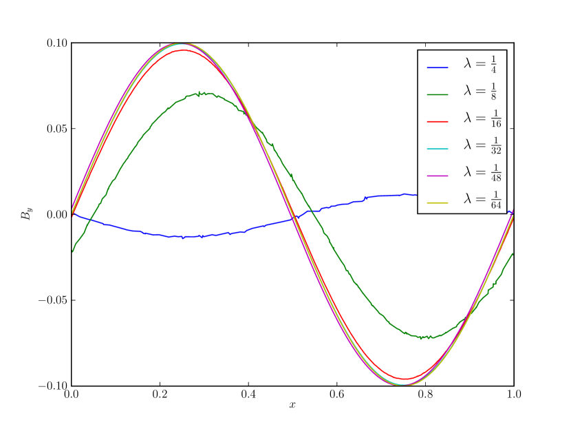
Figure 2.— Circularly polarized Alfvén waves after five box crossings with resolutions given by the legend. Note the rapid convergence of the higher resolution models.

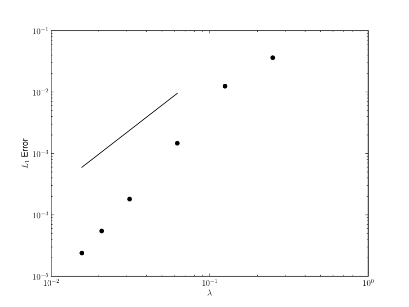
Figure 3.— $L_{1}$-norm errors for circularly polarized Alfvén waves run with resolution $\lambda$ after five box crossings. The plotted reference slope is 2.

For our next test of MHD, we run finite-amplitude, circularly polarized, Alfvén plane waves using the parameters from Tóth (2000) in a cubic domain with periodic boundary conditions, with the propagation direction parallel to the x-axis. This is equivalent to $\alpha=0$ in the formalism of Tóth (2000). Specifically, the initial conditions are $\rho=1.0$, $V_{x}=0.0$, $B_{x}=1.0$, $V_{y}=0.1\sin(2\pi x)=B_{y}$, $V_{z}=0.1\cos(2\pi x)=B_{z}$, $P=0.1$, and $\gamma=5/3$. The wave is propagated five wavelengths, returning to its original position. The solutions shown in Figure 2 show that at low resolution, the wave is strongly damped, while as resolution increases the wave rapidly converges. Figure 3 shows the $L_{1}$ norm errors, which converge faster than second order.

3.3. Shock Tubes

Table 1Shock Tube Left and Right States

Test	$\rho$	$V_{x}$	$V_{y}$	$V_{z}$	$P$	$B_{x}$	$B_{y}$	$B_{z}$
Sod Left	1	0	0	0	1	0	0	0
Sod Right	0.125	0	0	0	0.1	0	0	0
Brio-Wu Left	1	0	0	0	1	0	1	0
Brio-Wu Right	0.125	0	0	0	0.1	0	-1	0
RJ2a Left	1.08	1.2	0.01	0.5	0.95	$2/\sqrt{4\pi}$	$3.6/\sqrt{4\pi}$	$2/\sqrt{4\pi}$
RJ2a Right	1	0	0	0	1	$2/\sqrt{4\pi}$	$4/\sqrt{4\pi}$	$4/\sqrt{4\pi}$
RJ4d Left	1	0	0	0	1	0.7	0	0
RJ4d Right	0.3	0	0	1	0.2	0.7	0.7	1
F6 Left	0.5	0	2	0	10	2	2.5	0
F6 Right	0.1	-10	0	0	0.1	2	2.5	0
RJ1a Left	1	10	0	0	20	$5/\sqrt{4\pi}$	$5/\sqrt{4\pi}$	0
RJ1a Right	1	-10	0	0	1	$5/\sqrt{4\pi}$	$5/\sqrt{4\pi}$	0

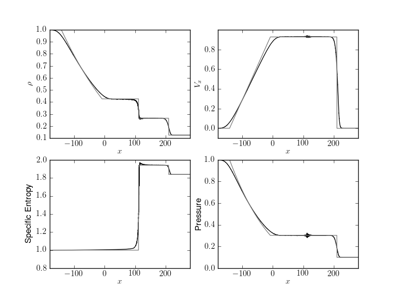
Figure 4.— Sod (1978) shock tube, run with mass-based refinement, equivalent to a Lagrangian method such as SPH. The $x$-axis is denoted in units of $\lambda$ of the initial left state density. Phurbas result in black, reference solution in gray.

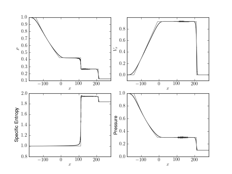
Figure 5.— Sod (1978) shock tube run with constant spatial resolution. Phurbas result shown in black, reference solution in gray.

To test performance on supersonic and super-Alfvénic problems, we set up several shock tube problems. We used the parameters given in Table 1 on long rectangular domains with periodic boundaries. A spatially constant resolution criterion $\lambda$ allows comparison to grid based codes, while an appropriately density dependent resolution criterion allows comparison to other Lagrangian methods. For the constant $\lambda$ tests we denote the distance along the long axis of the domain in units of $\lambda$.

3.3.1 Sod Shock Tube

We first run the classic Sod (1978) shock tube, in gas with $\gamma=7/5$ on a domain of size $64\times 1\times 1$ units. A smooth transition between the left and right states with a width of $0.3$ units is described with a fifth-order spline. In the first version of this test we use a refinement criteria $\lambda=0.125\rho^{1/3}$ that yields a constant mass per resolution element (that is, per region with volume of $4/3\pi\lambda^{3}$). This is in effect the resolution criterion used by SPH. In Figure 4 the solution at time $t=13.8$ is shown. For this test the x axis on the plot is denoted in units of $\lambda$ in the left initial state. Unlike SPH, Phurbas supports more general refinement criteria. As a simple example, we ran the same Sod test problem with spatially constant resolution $\lambda=0.125$. Figure 5 shows the result at time $t=15$. The result is generally very similar to the result with mass-based refinement, with the main change being that the shock is thinner, as the local resolution is higher in the constant-refinement case. In either case, the shock speed is reasonably well reproduced.

3.3.2 MHD Shock Tubes

We next perform a suite of MHD shock tube tests, selecting from the large set of standard MHD Riemann problems used in the literature. To tabulate reference solutions, we have used Athena (Stone et al., 2008) at high resolution in 1D. The first test we show is the classical Brio-Wu 1988 shock tube test, which is a standard problem, though not particularly stringent. The test shown in Figure 2a of Ryu & Jones (1995, denoted RJ2a) provides a more complete test of the appearance of the various possible MHD discontinuities. Ryu & Jones (1995) in their Figure 4d show a test (denoted RJ4d) of other discontinuities. The problem described by Falle (2002) in his Figure 6 (denoted F6) is specifically used to demonstrate shock errors in non-locally-conservative methods. Finally, the test shown in Figure 6 of Dai & Woodward (1994), as well as in Figure 1a of Ryu & Jones (1995, denoted RJ1a) is commonly used as a stringent test of ${\nabla\!\cdot\!\textbf{\em B}}$ errors in shocks, and in the case of Phurbas demonstrates the effects of local non-conservation errors associated with strong MHD shocks. Note that with the exception of the Brio-Wu test, all these MHD shock tube tests use an adiabatic gas with $\gamma=5/3$.

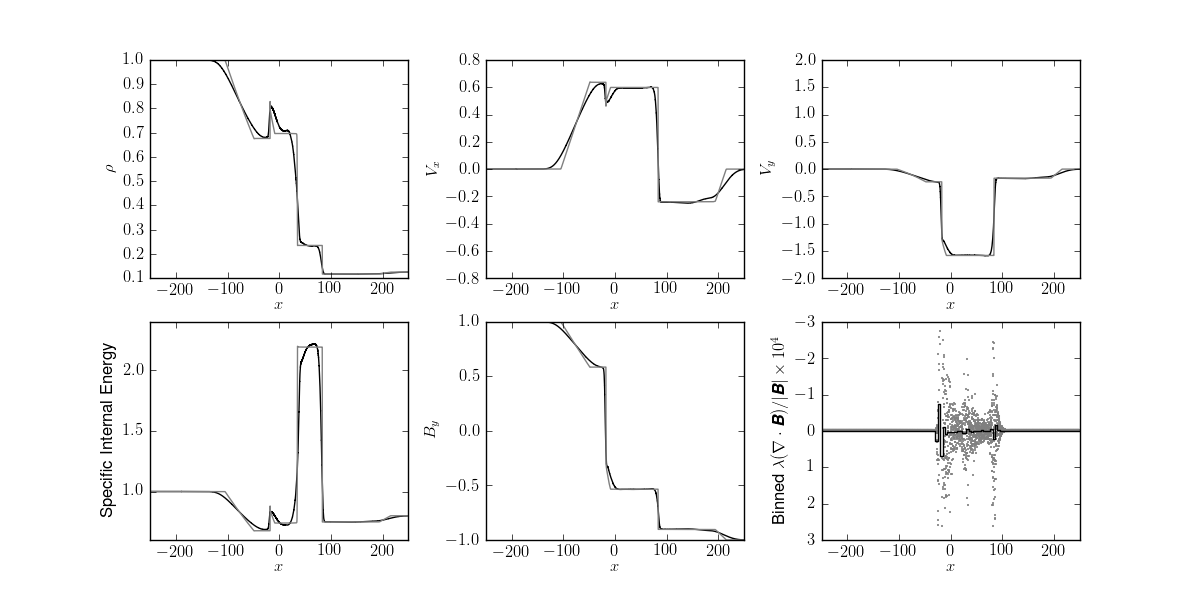
Figure 6.— Brio-Wu 1988 shock tube solution with Phurbas solution in black, and high-resolution Athena solution in gray. Lower right panel: One in ten unbinned values of ${\nabla\!\cdot\!\textbf{\em B}}$ as grey points, binned values as black steps.

Brio-Wu

The Brio-Wu 1988 shock tube (see Table 1) is an MHD analog to the Sod shock tube problem. We set up this test in gas with $\gamma=2$, on a fully periodic domain of $128\times 1\times 1$ units, with constant resolution $\lambda=0.125$. A smooth transition between the left and right states with a width of $3$ units was produced with a cosine function. The width of the transition region was chosen to avoid excessive start-up transients.

As the problem was run in two mirror images in a periodic volume, only half of the periodic volume used is shown in Figure 6, with the $x$-axis labeled in $\lambda$ units, at time $t=7.3$. The solution captures the fundamental features of the problem, including, from left to right, the rarefaction fan, the compound wave, the contact discontinuity, the slow shock, and the fast rarefaction wave.

The final panel of Figure 6 shows a measure of the effect of ${\nabla\!\cdot\!\textbf{\em B}}$. Here the quantity $\lambda({\nabla\!\cdot\!\textbf{\em B}})/|{\textbf{\em B}}|$ is the fractional magnetic field error on the scale of $\lambda$. Grey points in this panel show the raw values of this quantity, with maximum magnitude $10^{-3}$. However, the scatter is very symmetric, indicating that most of it can be attributed to the truncation error in the approximation of ${\nabla\!\cdot\!\textbf{\em B}}$ itself. To extract the coherent skew from zero, we plot the data binned in bins with width $\lambda$ as the black step curve, demonstrating that the normalized ${\nabla\!\cdot\!\textbf{\em B}}$ errors are less than $10^{-4}$.

The Athena solution that we compare our result to, as well as the usually accepted numerical solutions to the Brio-Wu problem, show a compound wave structure, seen at $x\approx-25$ in Figure 6. This structure should not formally exist (Falle & Komissarov, 2001), but most multidimensional numerical methods, including Phurbas, show it as part of the solution.

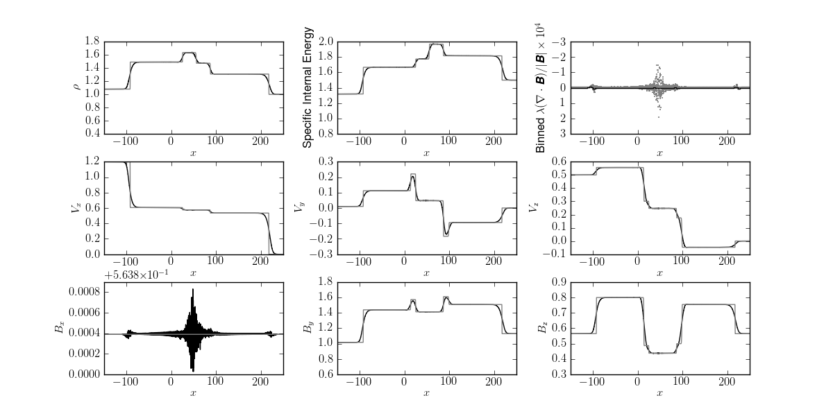
Figure 7.— Ryu & Jones (1995) test from their Figure 2a (model RJ2a). High resolution Athena solutions are shown in gray, while the normalized $\nabla\cdot B$ is shown as gray points, and the binned values are shown in black steps. One in ten particles is plotted in the ${\nabla\!\cdot\!\textbf{\em B}}$ scatter.

RJ2a

The test shown in Figure 2a of Ryu & Jones (1995) (also see Dai & Woodward (1994) Table 3a) is shown in Figure 7 at time $t=12$. Initial conditions for this test are listed in Table 1 as RJ2a. This test is otherwise set up in the same manner and on the same domain as the Brio-Wu test. A high resolution solution was computed with Athena for comparison. As Stone et al. (2008) point out, this test is particularly interesting because it requires modeling a fast magnetosonic shock and a rotational discontinuity in each direction of propagation, as well as a contact discontinuity in the center. No visible ringing is seen at the shocks. The largest coherent ${\nabla\!\cdot\!\textbf{\em B}}$ errors are also seen near the fast shocks, but the largest scatter in particle ${\nabla\!\cdot\!\textbf{\em B}}$ values is located at the contact discontinuity.

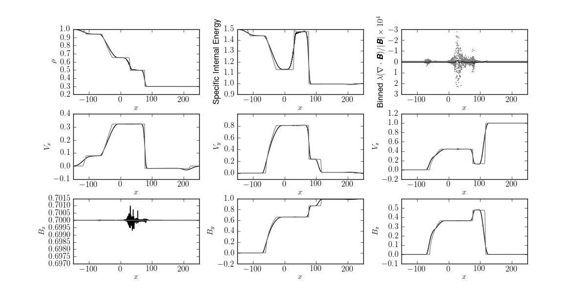
Figure 8.— Ryu & Jones (1995) test from their Figure 4d (model RJ4d). High resolution Athena solution shown in gray, while the normalized ${\nabla\!\cdot\!\textbf{\em B}}$ is shown as gray points, and the binned values are shown in black steps. One in ten particles plotted in ${\nabla\!\cdot\!\textbf{\em B}}$ scatter.

RJ4d

The test shown in Figure 4d of Ryu & Jones (1995) is shown in Figure 8 at time $t=11.5$. This test was run with the same computational domain and resolution as the previous test but with the left and right states listed in Table 1 as test RJ4d. A small overshoot can be seen on the leftmost rarefaction wave. This is a result of the bulk viscosity of the scheme.

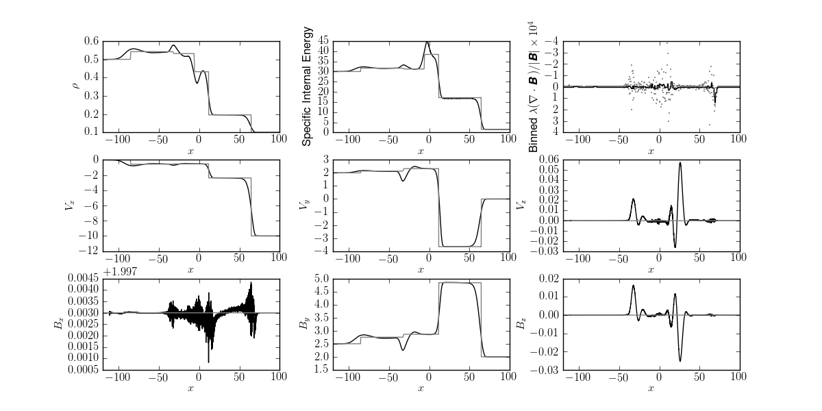
Figure 9.— Falle (2002) test from their Figure 6 (our test F6), which was used to demonstrate an error in the ZEUS algorithm. High resolution Athena solution shown in gray, while the normalized ${\nabla\!\cdot\!\textbf{\em B}}$ is shown as gray points, and the binned values are shown in black steps. One in ten particles is plotted in ${\nabla\!\cdot\!\textbf{\em B}}$ scatter.

F6

The test shown by Falle (2002) in his Figure 6 is shown in Figure 9 at time $t=2.9$. This test was used to show an error in the ZEUS (Stone & Norman, 1992) solution. The initial states are listed in Table 1 as test F6 and the problem was run in a domain of $64\times 1\times 1$ units with $\lambda=0.25$. Fixed boundaries were used in the $x$ direction and periodic boundaries in the $y$ and $z$ directions. Compared to the nonconservative ZEUS result shown in Falle (2002) the slow shock is captured more accurately. At this resolution, the slow shock and the contact discontinuity directly behind it have not yet separated, and the bulk viscosity of the scheme is causing an undershoot in density at the foot of the contact discontinuity. The left-going features also show overshoots in density and specific internal energy that are initial transients caused by the bulk viscosity. These effects are not however due to significant nonconservation errors.

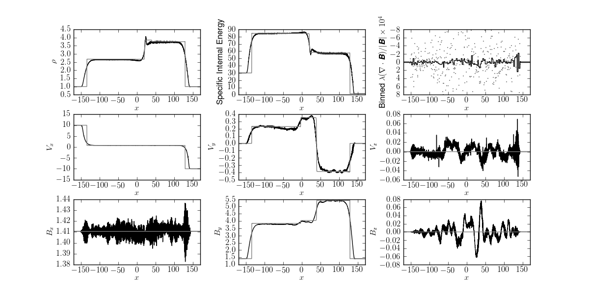
Figure 10.— Riemann problem test shown by Ryu & Jones (1995) in their Figure 1a, run without elliptic projection ${\nabla\!\cdot\!\textbf{\em B}}$ correction. High resolution Athena solution shown in gray, while the normalized ${\nabla\!\cdot\!\textbf{\em B}}$ is shown as gray points, and the binned values are shown in black steps. One in ten particles is plotted in the ${\nabla\!\cdot\!\textbf{\em B}}$ scatter.

RJ1a

The test shown by Dai & Woodward (1994) in their Figure 6, is shown in Figure 10 at time $t=3.5$. This test also appears in Ryu & Jones (1995) in their Figure 1a, in Table 6 of Tóth (2000), and in Mignone et al. (2010). In the latter two it is used as a demonstration of ${\nabla\!\cdot\!\textbf{\em B}}$ errors. We show this problem here as a test of the technique used in Phurbas to handle ${\nabla\!\cdot\!\textbf{\em B}}$, though we expect that the strength of the shocks in this problem lies outside of the intended use regime of Phurbas. A computational volume $64\times 1\times 1$ units was used, with fixed value boundaries in the $x$ direction, and periodic boundaries in the $y$ and $z$ directions with left and right states listed in Table 1 as test RJ1a. As Dai & Woodward (1994) show, the solution consists of a right going fast shock with Mach number 6.54, a left going fast shock with Mach number 2.54, a slow shock, a slow rarefaction, and a contact discontinuity. Phurbas shows a $\nabla\cdot\mathbf{B}$ error of a few parts in $10^{4}$ in the region lying between the two fast shocks.

3.4. Kelvin-Helmholtz Instability

As an example of multidimensional smooth flow with bulk motions, we demonstrate the performance of Phurbas on three-dimensional Kelvin-Helmholtz instability. Recently Kelvin-Helmholtz instability has attracted significant discussion following the demonstration by Agertz et al. (2007) that some SPH formulations fail to show the growth of the instability in a particular test problem. A number of works have discussed aspects of Kelvin-Helmholtz instability in numerical methods used in astrophysics, particularly in Lagrangian schemes (Price, 2008; Wadsley et al., 2008; Cha et al., 2010; Heß & Springel, 2010; Springel, 2010a; Read et al., 2010; Junk et al., 2010; Valcke et al., 2010; Springel, 2010b; Robertson et al., 2010; Springel, 2011).

In the terminology of Robertson et al. (2010) and Springel (2010b) we use a smoothed interface initial condition. However, unlike Springel (2010b) we choose a smoothing of the interface such that a closed-form algebraic expression can be computed for the first order, linear, perturbation theory prediction for the growth rate in an incompressible flow on an infinite domain. Wang et al. (2010) have derived such an analytic treatment, providing an exact analytic benchmark for the first time. From that work, we select an initial condition with an exponential smoothing. The initial condition for the Kelvin-Helmholtz test is as follows in coordinates where $x$ is parallel to the direction of flow, and $z$ is in the direction of slab symmetry. Density is given by

$$\rho=\left\{\begin{array}[]{ll}\rho_{1}-\rho_{m}e^{\frac{y-1}{L}}&\mbox{ if }1>y>0\\ \rho_{2}+\rho_{m}e^{\frac{-y+1}{L}}&\mbox{ if }2>y>1\\ \rho_{2}+\rho_{m}e^{\frac{-(3-y)}{L}}&\mbox{ if }3>y>2\\ \rho_{1}-\rho_{m}e^{\frac{-(y-3)}{L}}&\mbox{ if }4>y>3,\end{array}\right.$$ (1)

where $\rho_{1}=1.0$, $\rho_{2}=1.1$, $\rho_{m}=(1/2)(\rho_{1}-\rho_{2})$, and $L=0.025$. The velocity field is given by a similar smoothed profile with a perturbation in the $x$ direction

$$V_{x}=\left\{\begin{array}[]{ll}U_{1}-U_{m}e^{\frac{y-1}{L}}&\mbox{ if }1>y>0\\ U_{2}+U_{m}e^{\frac{-y+1}{L}}&\mbox{ if }2>y>1\\ U_{2}+U_{m}e^{\frac{-(3-y)}{L}}&\mbox{ if }3>y>2\\ U_{1}-U_{m}e^{\frac{-(y-3)}{L}}&\mbox{ if }4>y>3,\end{array}\right.$$ (2)

where $U_{1}=0.5$, $U_{2}=-0.5$, $U_{m}=(1/2)(U_{1}-U_{2})$, and a perturbation in the $y$ direction

$$V_{y}=\delta v\sin(4\pi x)\left\{\begin{array}[]{ll}\exp(4\pi(y-1))&\mbox{ if }1>y>0\\ \exp(4\pi(-y+1))&\mbox{ if }2>y>1\\ \exp(4\pi(-(3-y))&\mbox{ if }3>y>2\\ \exp(4\pi(-(y-3))&\mbox{ if }4>y>3,\end{array}\right.$$ (3)

where $\delta v=0.01$. Pressure is set to $2.5$, and $\gamma=5/3$.

To extract the growth of the velocity perturbation, we use a discrete convolution over the particles. We use this technique, as opposed to a discrete Fourier transform on gridded values, as the discrete convolution maps more directly to the meshless Phurbas discretization. We define the magnitude of the unstable $y$-velocity mode

$$M=2\left[\left(\frac{\sum{s_{i}}}{\sum{d_{i}}}\right)^{2}+\left(\frac{\sum{c_{i}}}{\sum{d_{i}}}\right)^{2}\right]^{\frac{1}{2}},$$ (4)

where all the sums run over $N$ particles, and

$$s_{i} =\left\{\begin{array}[]{l l}V_{y}\sin(4\pi x)\exp(-4\pi|y-1|)&\mbox{ if }y<2\\ V_{y}\sin(4\pi x)\exp(-4\pi|(4-y)-1|)&\mbox{ if }y>2,\\ \end{array}\right.$$ (7)

$$c_{i} =\left\{\begin{array}[]{l l}V_{y}\cos(4\pi x)\exp(-4\pi|y-1|)&\mbox{ if }y<2\\ V_{y}\cos(4\pi x)\exp(-4\pi|(4-y)-1|)&\mbox{ if }y>2,\\ \end{array}\right.$$ (10)

$$d_{i} =\left\{\begin{array}[]{l l}\exp(-8\pi|y-1|)&\mbox{ if }y<2\\ \exp(-8\pi|(4-y)-1|)&\mbox{ if }y>2.\\ \end{array}\right.$$ (13)

The domain is $4\times 1$ units with thickness $1/32$, $1/64$, or $1/128$, simulated with uniform target resolutions $\lambda=1/64$, $1/128$, and $1/256$.

In Figure 11 the developed state of the highest resolution run is shown, while Figure 12 shows the growth of the unstable $y$-direction velocity mode and the maximum $y$-direction kinetic energy. The linear perturbation theory predictions from Wang et al. (2010) for the growth rate of the mode amplitude and the maximum $y$-direction kinetic energy are also plotted as a guide, but due to the periodic domain, compressibility, and finite perturbation magnitude we cannot expect the result to exactly follow this curve. However, clear convergence toward the linear theory can be seen as resolution increases. A more sophisticated, multiple code verification study, circumventing the limitations of the incompressible theory comparison for a similar problem, will be presented in a separate publication.

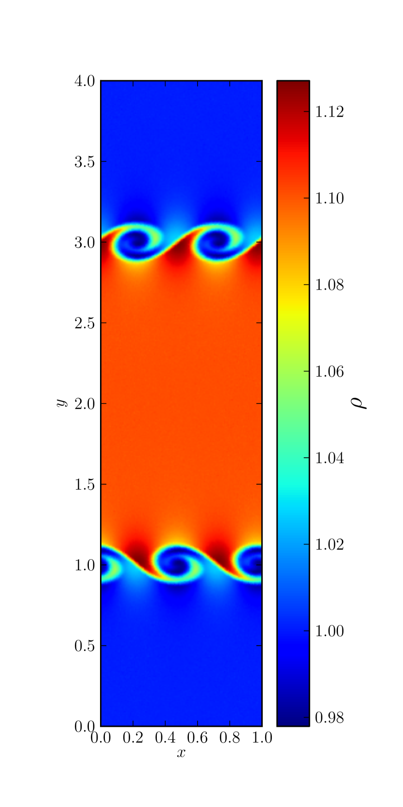
Figure 11.— Kelvin-Helmholtz instability test presented at the highest resolution used here ($\lambda=1/256$). A density slice is shown at t=2.52.

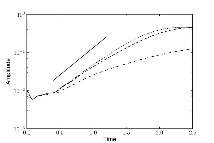
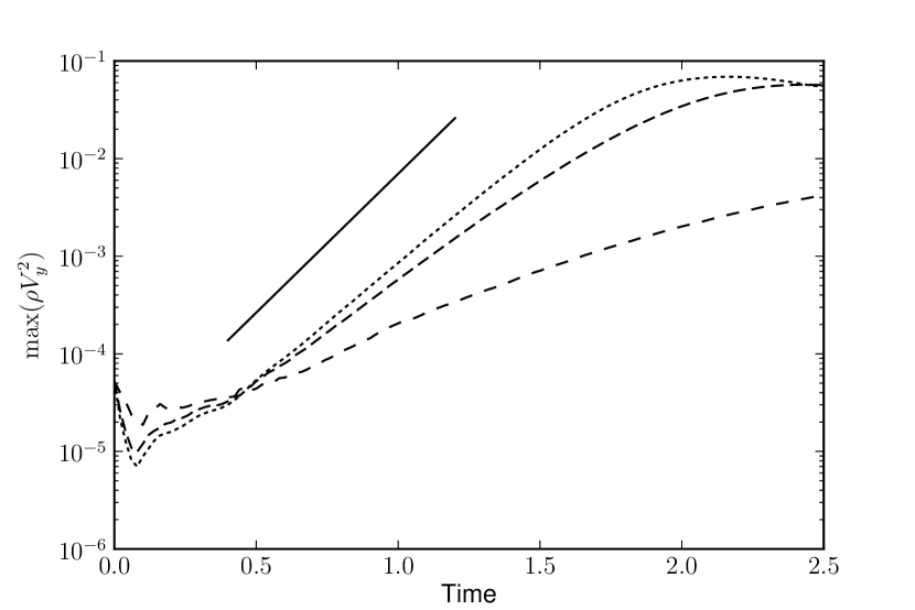
Figure 12.— Left: Kelvin-Helmholtz instability mode growth for models with $\lambda=1/64$ (dashes), $1/128$ (tight-spaced dashes), and $1/256$ units (dotted), compared to the predicted growth rate (solid) from the linear, incompressible theory derived by Wang et al. (2010). Right: Maximum $y$-direction kinetic energy for the same runs, again compared to the predicted growth rate from linear, incompressible theory.

3.5. Magnetorotational Instability in a Cylinder

The magnetorotational instability (MRI; Balbus & Hawley, 1991) is thought to be an important mechanism for driving turbulence in protoplanetary disks (Balbus & Hawley, 1998). We have performed a test similar to one done by Flock et al. (2010) to examine the growth rate of MRI during its linear phase. For this test, we remove the background Keplerian shear flow from the velocity field, and evolve only the perturbations to the initial steady state velocity. That is, the velocity field we evolve and fit in this test is ${\textbf{\em V}}^{\prime}={\textbf{\em V}}-\Omega r\hat{\mathsf{\phi}}$ where $r$ is the cylindrical radius from the point (0.5,0.5), $\Omega=r^{-1.5}$ is the Keplerian angular velocity and $\hat{\mathsf{\phi}}$ is the unit vector in the azimuthal direction. Additionally, to ensure that the magnetic field configuration we study is consistent between resolutions, we solve only for perturbations from the initial magnetic field configuration. Solving only for the perturbations is particularly useful here as the MRI grows fastest where the orbital timescale is smallest.

The magnetic field configuration used in this test, an annulus of uniform vertical field, is chosen to artificially cut off the growth of MRI at a finite radius. Ensuring that the MRI is cleanly shut off and that the annulus is represented in a constant manner allows clearer measurements of the convergence of the growth rate in the magnetized annulus. The domain is an annulus with radius ranging from 0.08 to 0.32 and height 0.0375 units. The vertical boundaries are periodic. The inner and outer radial boundaries are fixed-value, arranged by preventing time evolution for particles with radius greater than 0.3 or less than 0.1. The initial density is 1.0 everywhere. A vertical magnetic field is imposed with radial profile $B_{z}(r)=B_{0}b_{p}(r)$, where $B_{0}=0.0824$ and

$$b_{p}(r)=\left\{\frac{1}{2}+\frac{1}{2}\tanh\left(5-\sin\left[\frac{2\pi(r-0.05)}{0.2}\right]\right)\right\},$$ (15)

which gives a magnetized annulus. The sound speed in the magnetized annulus was set to $c_{s}=0.824$, and the internal energy in the non-magnetized region adjusted so that the total pressure (thermal plus magnetic) is constant. The radial velocity is perturbed with

$$V_{r}(z)=10^{-5}c_{s}b_{p}(r)\cos(2\pi z/0.1).$$ (16)

Spatially constant resolutions of $\lambda=1/240$, $\lambda=1/320$, and $\lambda=1/400$ were used corresponding to $\lambda=1/9\lambda_{\mathrm{MRI}}$, $\lambda=1/12\lambda_{\mathrm{MRI}}$, $\lambda=1/15\lambda_{\mathrm{MRI}}$ where $\lambda_{\mathrm{MRI}}=0.0375$ is the wavelength of the fastest growing MRI mode at $r=0.17$.

We then measure the growth of the most unstable mode at $r=0.17$. Figure 13 shows the radial magnetic field configuration achieved at time $0.94$ (or $2.13$ orbits at $r=0.17$) for all three resolutions. To calculate the mode amplitude $M$, we use a convolution defined directly on the particles, instead of gridding and Fourier transforming the data. The motivations are the same as when this procedure was used for the Kelvin-Helmholtz test. In this case,

$$M=\left[\left(\frac{\sum{s_{i}}}{\sum{d_{i}}}\right)^{2}+\left(\frac{\sum{c_{i}}}{\sum{d_{i}}}\right)^{2}\right]^{\frac{1}{2}},$$ (17)

where all sums run over the $N$ points, and

$$s_{i} =B_{r,i}\sin\left(\frac{2\pi}{0.0375}z_{i}\right)\exp\left(-\frac{(r_{i}-r_{0})^{2}}{\sigma^{2}}\right),$$ (18)

$$c_{i} =B_{r,i}\cos\left(\frac{2\pi}{0.0375}z_{i}\right)\exp\left(-\frac{(r_{i}-r_{0})^{2}}{\sigma^{2}}\right),$$ (19)

$$d_{i} =\exp\left(-\frac{(r_{i}-r_{0})^{2}}{\sigma^{2}}\right).$$ (20)

The chosen width of the convolution $\sigma=2.7\times 10^{-6}$ minimizes the radial range that influences the measurement, while still giving sufficiently low sampling noise.

We plot the evolution of the mode amplitude in Figure 14 together with the maximum growth rate of $\exp(0.75\Omega)$ predicted by a linear perturbation analysis of vertical field MRI. The modeled growth rates are reasonably consistent with the prediction from the linear analysis for the fastest growing mode. Importantly, in the context of the findings of Flock et al. (2010), where spuriously high growth rates were observed, we find growth rates slightly lower than the theoretical maximum value.

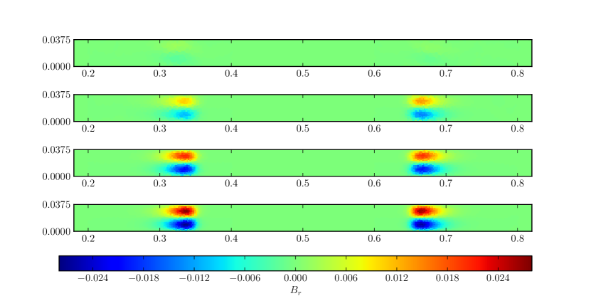
Figure 13.— Linear phase growth of MRI shown via azimuthal field slices at time 0.94 for resolutions (from top to bottom) of $\lambda=1/160,1/240,1/320$, and $1/400$.

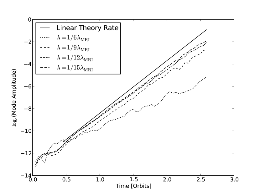
Figure 14.— Linear phase growth of MRI shown for the mode amplitude given by equation (17) at $r=0.17$ for the resolutions $\lambda$ given in the legend, compared to the growth rate predicted by linear theory.

4. Summary and Discussion

4.1. Effective Resolving Power

To determine if Phurbas can be used for practical computations, we need to establish some guidelines for its relative ability to resolve particular phenomena. This should be done cautiously, as different classes of algorithms have different properties in each flow regime. An equivalence or difference between algorithms in one regime may not hold across different regimes. In any case, it is expected that an unstructured mesh or unstructured meshless method will have a lower effective resolution than a structured mesh method. This is because a given number of resolving elements can represent the largest possible set of wavelengths when they are arranged in a regular manner. Given these caveats, we can compare the test results that we have presented here to examples computed with Eulerian, mesh-based schemes.

The first example is the circularly polarized Alfvén wave test. The lowest resolution, three-dimensional, Athena results in a rectangular domain published in Stone et al. (2008, Fig. 33) correspond to $20$ and $39$ cells per wavelength, computed with third order spatial reconstruction and HLLD fluxes. The Phurbas results on this test at $\lambda=1/8$ and $\lambda=1/16$ of a wavelength appear to roughly equal the accuracy of the $20$ and $39$ cells per wavelength Athena results in the sense that the final amplitude of the wave in the Phurbas results is closer to the analytically correct value even though there are fewer resolution elements used per wavelength. This result should be interpreted cautiously, as the two codes have different and nonlinear numerical dissipation. Nevertheless, this can be interpreted to mean that the Phurbas effective resolution $\lambda$ is roughly equal to two Athena cells as a measure of resolution. (On average, there should be one particle in each volume of radius $\lambda$.) In this sense Phurbas with a third-order polynomial fit is competitive with a spatially third-order grid code.

A possibly more operationally useful comparison can be drawn from the results of the linear phase MRI growth test. Flock et al. (2010) claim that in the code Pluto (Mignone et al., 2007) with piecewise linear reconstructions and an HLLD Riemann solver, 10 cells per wavelength are required to resolve the growth of MRI. Our test in section 3.5 shows Phurbas requires $\sim 9$ $\lambda$ per MRI wavelength to resolve the growth. Thus, for this test we can say that one cell$\ \approx 1\lambda$. The algorithm used by Flock et al. (2010) has a stencil size of five cells, while Phurbas can be said to have a stencil size of $2r_{f}=4.6\lambda$, so the same rough proportionality holds between the two algorithms when expressed in terms of stencil size.

4.2. Advantages and Disadvantages

The main advantage of Phurbas is its Lagrangian nature. Eulerian codes suffer from numerical dissipation that varies with the speed and direction of the flow across the grid. Phurbas’s formulation cleanly avoids this behavior. For systems where the bulk velocity varies as a multiple or large fraction of the wave speeds, this means Phurbas can capture the flow with more uniform fidelity across the domain. Techniques that add an extra advection step to an Eulerian method (e.g. Masset, 2000; Johansen et al., 2009) can only efficiently handle simple flow geometries. Moreover, in Phurbas, the time step is only dependent on Galilean-invariant quantities. For flow with bulk velocities greater than the signal speeds that determine the Courant time step limit, Phurbas has a significant advantage in the number of time steps that must be computed to reach a given physical time.

The resolution criterion in Phurbas is spatially continuous, unlike in adaptive mesh refinement techniques, so there are no abrupt resolution jumps that can lead to undesirable artifacts. Also, due to the Lagrangian and meshless nature of the code, refined regions can be arbitrarily shaped and follow the flow with minimal creation and deletion of resolution elements.

As Phurbas formally computes strong solutions to the governing partial differential equations using a method-of-lines type approach, it is relatively simple, compared to Godunov methods for example, to switch to an alternate set of variables or even alternate equations. The central limitation is only that the equations should be amenable to the explicit Hermitian time integration used. However, changing the time integration scheme would not fundamentally alter the method.

A moving unstructured mesh or meshless method must win in terms of the Galilean invariance of the numerical diffusion, adaptivity, and the time step advantages, since the quality of the spatial derivatives on an unstructured set of discretization points is lower than for equivalent fits on a grid of points. For problems where the Lagrangian and adaptive nature of Phurbas is of no significant advantage, a grid-based method such as the Pencil Code (Brandenburg & Dobler, 2002) remains substantially more efficient.

4.3. Future Prospects

Several enhancements to Phurbas can be made, which we briefly mention here.

• The Phurbas discretization is very flexible in how it can incorporate governing equations other than ideal MHD. Implementing non-ideal MHD is relatively simple with forward-time-centered-space viscosity and resistivity operators.

• Self-gravity can be implemented using the existing GADGET-2 tree algorithm and particle masses derived from a local Voronoi tessellation.

• Passive tracer particles and interacting dust particles can be added in a straightforward manner, using the spatial fitting and time integration methods used for gas particles.

• In the moving least squares procedure the choice of least squares error and Cartesian polynomial functions for the fitting procedure is not obviously the ideal choice, and alternate fitting procedures should be explored. These could include those with a basis that can be used to minimize the variation or oscillation of the fitted function, and fitting the magnetic field using a set of divergence-free basis functions (McNally, 2011).

• Least-squares minimization itself does not appear to be a unique choice, and less computationally intensive gradient approximation procedures could be used.

• Non-Lagrangian particle trajectories can be added, using similar logic to the steering of Voronoi cell generating centers in Springel (2010a). This could reduce the number of particle additions and deletions, and hence diffusivity in shear flows.

• An improved void check algorithm could reduce the number of redundant particle creation requests, minimizing the potentially expensive step of pruning of the proposed particle addition list.

• A diffusion with properties similar to a hyperdiffusion would be of great advantage if applied to the density and internal energy fields to smooth out the smallest scale structures. The challenge of this enhancement is to find an approximation with sufficiently robust conservation properties.

Evidently, there are many possible alterations and extensions that can be made to Phurbas that will significantly alter both the nature of the scheme and the capabilities of the code. We believe that Phurbas is not just a new method for MHD, but one of the first practical examples of a new class of schemes for mathematical modeling of similar physical problems.

Appendix A Dispersion Relation and Modified Waves

The test in §3.1 is a convergence test to the solution of the linearized version of the modified MHD equations that Phurbas solves. We derive here the dispersion relation and solutions in the cases used in the convergence test. We start with the MHD mass, momentum, and induction equations, with a bulk viscosity term $\rho\nabla(\zeta\nabla\cdot\mathbf{V})$ added to the momentum equation,

$$\partial_{t}\rho+\rho\nabla\cdot\mathbf{V} =0$$ (A1)

$$\rho\partial_{t}\mathbf{V}+\nabla P-(\nabla\times\mathbf{B})\mathbf{B}+\rho\nabla(\zeta\nabla\cdot\mathbf{V}) =0$$ (A2)

$$\partial_{t}\mathbf{B}+\nabla\times(\mathbf{V}\times\mathbf{B}) =0,$$ (A3)

and for adiabatic gas we also use an energy equation

$$\partial_{t}\left(\frac{P}{\rho^{\gamma}}\right)=0.$$ (A4)

In these equations, $\rho$ is density, $\mathbf{V}$ is velocity, $P$ is pressure, $\mathbf{B}$ is magnetic field, and $\gamma$ is the adiabatic index. Linearizing, and taking the viscosity $\zeta$ as constant we obtain

$$\partial_{t}\rho+\rho_{0}\nabla\cdot\mathbf{V} =0$$ (A5)

$$\rho_{0}\partial_{t}\mathbf{V}+\nabla P-(\nabla\times\mathbf{B})\times\mathbf{B}_{0}+\rho_{0}\zeta\nabla(\nabla\cdot\mathbf{V}) =0$$ (A6)

$$-\partial_{t}\mathbf{B}+\nabla\times(\mathbf{V}\times\mathbf{B}) =0$$ (A7)

$$\partial_{t}\left(\frac{P}{P_{0}}-\frac{\gamma\rho}{\rho_{0}}\right) =0$$ (A8)

where subscripts $0$ indicate background values, and unsubscripted variables are fluctuations. Substituting the form $\exp(i(\mathbf{k}\cdot\mathbf{r}-\omega t))$ as a dependence for all variables to search for wave solutions gives

$$-\omega\rho+\rho_{0}\mathbf{k}\cdot\mathbf{V} =0$$ (A9)

$$-\omega\rho_{0}\mathbf{V}+\mathbf{k}P-(\mathbf{k}\times\mathbf{B})\times\mathbf{B}_{0}+\zeta i\omega\mathbf{k}(\mathbf{k}\cdot\mathbf{V}) =0$$ (A10)

$$\omega\mathbf{B}+\mathbf{k}\times(\mathbf{V}\times\mathbf{B}_{0}) =0$$ (A11)

$$-\omega\left(\frac{P}{P_{0}}-\frac{\gamma\rho}{\rho}\right) =0$$ (A12)

Solving these transformed version of the mass, induction, and equation of state for the perturbed variables gives

$$\rho =\rho_{0}\frac{\mathbf{k}\cdot\mathbf{V}}{\omega}$$ (A13)

$$P =\gamma P_{0}\frac{\mathbf{k}\cdot\mathbf{V}}{\omega}$$ (A14)

$$\mathbf{B} =\frac{(\mathbf{k}\cdot\mathbf{V})\mathbf{B}_{0}-(\mathbf{k}\cdot\mathbf{B}_{0})\mathbf{V}}{\omega}$$ (A15)

We can then substitute these into the linearized momentum equation to yield

$$\left[\omega^{2}-\frac{(\mathbf{k}\cdot\mathbf{B}_{0})^{2}}{\rho_{0}}\right]\mathbf{V}=$$

$$\left\{\left[\frac{\gamma P_{0}}{\rho_{0}}+\frac{\mathbf{B}_{0}^{2}}{\rho_{0}}\right]\mathbf{k}-\frac{(\mathbf{k}\cdot\mathbf{B}_{0})}{\rho_{0}}\mathbf{B}_{0}\right\}(\mathbf{k}\cdot\mathbf{V})-\frac{(\mathbf{k}\cdot\mathbf{B}_{0})(\mathbf{V}\cdot\mathbf{B}_{0})}{\rho_{0}}\mathbf{k}-\zeta i\omega\mathbf{k}(\mathbf{k}\cdot\mathbf{V})$$ (A16)

Substituting in the Alfvén and sound speeds

$$\mathbf{V}_{A}=\sqrt{\frac{\mathbf{B}_{0}^{2}}{\rho_{0}}}\hat{\mathbf{B}}_{0},\qquad V_{S}=\sqrt{\frac{\gamma P_{0}}{\rho_{0}}}$$ (A17)

we obtain

$$\left[\omega^{2}-(\mathbf{k}\cdot\mathbf{V}_{A})^{2}\right]\mathbf{V}=$$

$$\left\{(V_{s}^{2}+V_{A}^{2})\mathbf{k}-(\mathbf{k}\cdot\mathbf{V}_{A})\mathbf{V}_{A}\right\}(\mathbf{k}\cdot\mathbf{V})-(\mathbf{k}\cdot\mathbf{V}_{A})(\mathbf{V}\cdot\mathbf{V}_{A})\mathbf{k}-\zeta i\omega\mathbf{k}(\mathbf{k}\cdot\mathbf{V}).$$ (A18)

We can now choose a propagation direction of the wave, the direction of the wave vector $\mathrm{k}$. The wave vector $\mathrm{k}$ is chosen to lie in the $x-z$ plane, at an angle $\theta$ clockwise from the $z$-axis. This gives

$$[\omega^{2}-k^{2}V_{A}^{2}\cos^{2}\theta]\mathbf{V}=$$

$$\left\{(V_{s}^{2}+V_{A}^{2})\mathbf{k}-\hat{\mathbf{z}}|k|V_{A}^{2}\cos\theta\right\}(\mathbf{k}\cdot\mathbf{V})-k^{2}\mathbf{V}_{A}\cos\theta(\mathbf{V}\cdot\mathbf{V}_{A})-\zeta i\omega\mathbf{k}(\mathbf{k}\cdot\mathbf{V}).$$ (A19)

Upon transforming this into a matrix eigenvalue problem, and solving for the eigenvectors $\mathbf{V}$ one obtains expressions for the eigenvalues, which can be solved for $\omega$. Unfortunately, we have only found analytic solutions for two special cases of the propagation direction $\theta$. These cases are used to test the convergence of our scheme. For propagation perpendicular to the background magnetic field $\mathbf{B}_{0}$, $\theta=\pi/2$ and the first eigenvalue corresponds to a magnetoacoustic wave, with speed given by $\mathfrak{Re}(\omega)/k=\sqrt{|k^{2}\zeta^{2}/4-(V_{A}^{2}+V_{s}^{2})|}$, and attenuation given by $\mathfrak{Im}(\omega)=ik^{2}\zeta/2$. For propagation in the direction of the background magnetic field $\mathbf{B}_{0}$, $\theta=0$ and the first eigenvalue corresponds to a sound wave, with speed given by $\mathfrak{Re}(\omega)/k=\sqrt{|k^{2}\zeta^{2}/4-(V_{s}^{2})|}$, and attenuation given by $\mathfrak{Im}(\omega)=ik^{2}\zeta/2$. In general, the shear Alfvén wave eigenmodes are unaffected by the addition of the bulk viscosity, as they do not involve compressive motions.

References

- Agertz et al. (2007) Agertz, O. et al. 2007, MNRAS, 380, 963, arXiv:astro-ph/0610051
- Balbus & Hawley (1991) Balbus, S. A., & Hawley, J. F. 1991, ApJ, 376, 214
- Balbus & Hawley (1998) Balbus, S. A., & Hawley, J. F. 1998, Rev. Mod. Phys., 70, 1
- Brandenburg & Dobler (2002) Brandenburg, A., & Dobler, W. 2002, Comp. Phys. Comm., 147, 471, arXiv:astro-ph/0111569
- Brio & Wu (1988) Brio, M., & Wu, C. C. 1988, J. Comp. Phys., 75, 400
- Cha et al. (2010) Cha, S.-H., Inutsuka, S.-I., & Nayakshin, S. 2010, MNRAS, 403, 1165
- Dai & Woodward (1994) Dai, W., & Woodward, P. R. 1994, J. Comp. Phys., 111, 354
- Falle (2002) Falle, S. A. E. G. 2002, ApJ, 577, L123, arXiv:astro-ph/0207419
- Falle & Komissarov (2001) Falle, S. A. E. G., & Komissarov, S. S. 2001, J. Plasma Phys., 65, 29
- Flock et al. (2010) Flock, M., Dzyurkevich, N., Klahr, H., & Mignone, A. 2010, A&A, 516, A26+, 0906.5516
- Heß & Springel (2010) Heß, S., & Springel, V. 2010, MNRAS, 406, 2289, 0912.0629
- Johansen et al. (2009) Johansen, A., Youdin, A., & Klahr, H. 2009, ApJ, 697, 1269, 0811.3937
- Junk et al. (2010) Junk, V., Walch, S., Heitsch, F., Burkert, A., Wetzstein, M., Schartmann, M., & Price, D. 2010, MNRAS, 407, 1933
- Maron et al. (2012) Maron, J., McNally, C. P., & Mac Low, M.-M. 2012, ApJS Accepted
- Masset (2000) Masset, F. 2000, A&AS, 141, 165, arXiv:astro-ph/9910390
- McNally (2011) McNally, C. P. 2011, MNRAS, 413, L76, 1102.4852
- Mignone et al. (2007) Mignone, A., Bodo, G., Massaglia, S., Matsakos, T., Tesileanu, O., Zanni, C., & Ferrari, A. 2007, ApJS, 170, 228, arXiv:astro-ph/0701854
- Mignone et al. (2010) Mignone, A., Tzeferacos, P., & Bodo, G. 2010, J. Comp. Phys., 229, 5896, 1001.2832
- Price (2008) Price, D. J. 2008, J. Comp. Phys., 227, 10040, 0709.2772
- Read et al. (2010) Read, J. I., Hayfield, T., & Agertz, O. 2010, MNRAS, 405, 1513, 0906.0774
- Robertson et al. (2010) Robertson, B. E., Kravtsov, A. V., Gnedin, N. Y., Abel, T., & Rudd, D. H. 2010, MNRAS, 401, 2463, 0909.0513
- Ryu & Jones (1995) Ryu, D., & Jones, T. W. 1995, ApJ, 442, 228, arXiv:astro-ph/9404074
- Sod (1978) Sod, G. A. 1978, J. Comp. Phys., 27, 1
- Springel (2005) Springel, V. 2005, MNRAS, 364, 1105, arXiv:astro-ph/0505010
- Springel (2010a) Springel, V. 2010a, MNRAS, 401, 791, 0901.4107
- Springel (2010b) Springel, V. 2010b, ARA&A, 48, 391
- Springel (2011) Springel, V. 2011, ArXiv e-prints, 1109.2218, accepted, To appear in Tessellations in the Sciences: Virtues, Techniques and Applications of Geometric Tilings, eds. R. van de Weijgaert, G. Vegter, J. Ritzerveld and V. Icke, Springer
- Stone et al. (2008) Stone, J. M., Gardiner, T. A., Teuben, P., Hawley, J. F., & Simon, J. B. 2008, ApJS, 178, 137, 0804.0402
- Stone & Norman (1992) Stone, J. M., & Norman, M. L. 1992, ApJS, 80, 791
- Tóth (2000) Tóth, G. 2000, J. Comp. Phys., 161, 605
- Valcke et al. (2010) Valcke, S., de Rijcke, S., Rödiger, E., & Dejonghe, H. 2010, MNRAS, 408, 71, 1006.1767
- Wadsley et al. (2008) Wadsley, J. W., Veeravalli, G., & Couchman, H. M. P. 2008, MNRAS, 387, 427
- Wang et al. (2010) Wang, L. F., Ye, W. H., & Li, Y. J. 2010, Phys. Plasmas, 17, 042103