Elliptical galaxy masses out to five effective radii: the realm of dark matter

Abstract

We estimate the masses of elliptical galaxies out to five effective radii using planetary nebulae and globular clusters as tracers. A sample of 15 elliptical galaxies with a broad variation in mass is compiled from the literature. A distribution function-maximum likelihood analysis is used to estimate the overall potential slope, normalisation and velocity anisotropy of the tracers. We assume power-law profiles for the potential and tracer density and a constant velocity anisotropy. The derived potential power-law indices lie in between the isothermal and Keplerian regime and vary with mass: there is tentative evidence that the less massive galaxies have steeper potential profiles than the more massive galaxies. We use stellar mass-to-light ratios appropriate for either a Chabrier/KTG (Kroupa, Tout & Gilmore) or Salpeter initial mass function to disentangle the stellar and dark matter components. The fraction of dark matter within five effective radii increases with mass, in agreement with several other studies. We employ simple models to show that a combination of star formation efficiency and baryon extent are able to account for this trend. These models are in good agreement with both our measurements out to five effective radii and recent SLACS measurements within one effective radii when a universal Chabrier/KTG initial mass function is adopted.

1. Introduction

There is strong evidence for the presence of dark matter in spiral galaxies where the rotation curves of their extended cold gas discs remain flat out to large radii. However, elliptical galaxies are generally free of cold gas so they lack an equivalent to the HI rotation curves of spiral galaxies. Furthermore, the stellar component of ellipticals is dominated by random motions so their kinematics are more difficult to model and the results are bedevilled by the mass-anisotropy degeneracy.

The confirmation of dark matter haloes surrounding elliptical galaxies has largely been confined to the brightest galaxies using either the X-ray emission of their hot gas (e.g. Loewenstein & White 1999; O’Sullivan & Ponman 2004; Humphrey et al. 2006; Johnson et al. 2009; Das et al. 2010) or strong lensing techniques (e.g. Treu & Koopmans 2004; Rusin & Kochanek 2005; Gavazzi et al. 2007; Koopmans et al. 2009; Auger et al. 2010a,Faure et al. 2011,Leier et al. 2011). Stellar dynamical studies from integrated light spectra can also be used to estimate dynamical masses (e.g. Gerhard et al. 2001; Cappellari et al. 2006; Thomas et al. 2007; Tortora et al. 2009), but such studies are generally limited to within a couple of effective radii, $R_{\rm eff}$.

To study the outer reaches of elliptical galaxies (i.e. beyond $\sim 2$ effective radii) requires distant tracers such as planetary nebulae (PNe) or globular clusters (GCs). In particular, PNe can be used to trace intermediate mass galaxies, whereas GCs and other mass probes are generally biased towards more massive systems. To make use of the larger mass range probed by the PNe, Douglas et al. (2002) developed a specialised instrument – the PNe Spectrograph (PN.S) – to study the kinematics of these tracers in elliptical galaxies. The early results of this project suggested a dearth of dark matter in ordinary ellipticals (Romanowsky et al. 2003). However, Dekel et al. (2005) showed that a declining velocity dispersion profile is consistent with a massive dark halo if the tracer anisotropy is radially biased. More recent work utilising PNe to trace the kinematics of intermediate mass ellipticals find that although there is some evidence for the presence of dark matter haloes, the fraction of dark matter (within $5R_{\rm eff}$) is somewhat lower than their higher mass analogues (e.g. Douglas et al. 2007; Napolitano et al. 2009; Napolitano et al. 2011). In addition, Napolitano et al. (2009) find that the dark matter halo concentrations (i.e $c_{200}$ or $c_{\rm vir}$) of these intermediate mass ellipticals are lower than $\Lambda$CDM predictions. However, estimating the dark matter halo mass and concentration at the virial radius requires a large extrapolation from the radial range of the current data ($5R_{\rm eff}\sim 0.1r_{\rm vir}$). In fact, Mamon & Łokas (2005) caution that extrapolation of dynamical studies within $\sim 5R_{\rm eff}$ to the virial radius are fraught with large uncertainties. A comparison between intermediate and high mass ellipticals is difficult as it is rare for both mass scales to be probed using the same method.

Whilst the overall mass of a galaxy can be derived using dynamical modelling of tracer kinematics, one must disentangle the stellar component in order to study the properties of the dark matter halo. However, incomplete knowledge of the initial mass function (IMF) inhibits this decomposition. While studies of our own Galaxy favour an IMF with a flattened slope below $0.5M_{\odot}$ (Scalo 1986; Kroupa et al. 1993; Chabrier 2003), near infrared spectroscopic studies of massive ellipticals find that the low mass slope of the IMF may become steeper (van Dokkum & Conroy 2010). Furthermore, several recent studies have suggested a mass-dependent IMF (e.g. Auger et al. 2010b; Treu et al. 2010).

Name	Type	Tracer	D	Ra	Dec	PA	$R_{\rm eff}^{\dagger}$	$L_{B}$	$V_{h}$	$\alpha^{\star}$	KS	$N(>2R_{\rm eff})$	$\left(V_{\rm rot}/\sigma\right)^{2}$	References
(NGC)			[kpc]	[deg]	[deg]	[deg]	[asec]	$10^{10}L_{B,\odot}$	kms-1
0821	E6	PNe	22.4	32.1	11.0	25	39	2.6	1735	3.3	1.0	55	0.10	Coc09†⋆
1344	E5	PNe	18.9	52.2	-31.2	167	46	1.8	1169	3.3	1.0	86	0.04	T05†;Coc09⋆
1399	E1	GC	19.0	54.6	-35.5	110	42	3.5	1442	2.7	0.6	444	0.01	Sag00†;Sch10⋆
1407	E0	GC	20.9	55.1	-18.6	60	57	4.7	1784	2.6	-	134	0.04	F06⋆; R09†
3377	E5	PNe	10.4	161.9	14.0	35	41	0.6	665	3.2	1.0	81	0.14	Coc09†⋆
3379	E1	PNe	9.8	162.0	12.6	70	47	1.4	889	3.3	1.0	89	0.03	Dou07;Coc09†⋆
4374	E1	PNe	17.1	186.3	12.9	135	72.5	5.0	1060	3.1	1.0	234	0.03	Coc09⋆; N11†
4486	E0	GC	17.2	187.7	12.4	160	105	7.3	1350	2.4	0.3	157	0.18	Cot01⋆; Cap06†; Mei07
4494	E1	PNe	15.8	187.9	25.8	0	53	2.2	1344	3.4	0.9	108	0.03	Coc09†⋆; N09
4564	E6	PNe	13.9	189.1	11.4	47	22	0.5	1142	3.4	0.3	29	1.00	Coc09†⋆
4636	E0	GC	15.0	190.7	2.7	145	108	2.7	906	2.6	-	105	0.02	Dir05⋆; Sch06†
4649	E2	GC/PNe	17.3	190.9	11.6	105	110	6.1	1117	2.8/3.2	1.0/0.8	61/68	0.42/0.04	H08⋆; L08†; T11⋆
4697	E6	PNe	10.9	192.2	-5.8	70	66	1.9	1241	3.4	1.0	180	0.10	De08†;Coc09⋆;Men09
5128	E/S0	GC/PNe	3.8	201.4	-43.0	35	300	2.7	541	3.4/3.5	-	156/323	0.10/0.38	W10†⋆; P04
5846	E0	PNe	23.1	226.6	1.6	70	81	4.0	1714	3.1	1.0	55	0.01	Cap06†;Coc09⋆

Table 1Parent galaxy properties - (1) Name of galaxy. (2) Type of tracer (GC or PNe). (3) Distance in Mpc. (4) and (5) Right ascension and declination. (6) Position angle. (7) Effective radius. (8) B band luminosity. The B band luminosity is derived from the de Vaucouleurs et al. (1991) apparent magnitudes and corrected for extinction according to Schlegel et al. (1998). (9) Heliocentric velocity. (10) Single power-law density index of tracers.(11) KS probability of approximate single power-law begin drawn from observed density model (12) Number of tracers beyond two effective radii. (13) Fraction of kinetic energy in rotation.(14) References. The source of the effective radii and tracer density distribution are indicated by the $\dagger$ and $\star$ symbols respectively: Cappellari et al. 2006 (Cap06), Coccato et al. 2009 (Coc09), Côté et al. 2001 (Cot01), de Lorenzi et al. 2008 (De08), Dirsch et al. 2005 (Dir05), Douglas et al. 2007 (Dou07), Forbes et al. 2006 (F06), Hwang et al. 2008 (H08), Lee et al. 2008 (L08), Mei et al. 2007 (Mei07), Méndez et al. 2009 (Men09), Napolitano et al. 2009 (N09), Napolitano et al. 2011 (N11), Peng et al. 2004 (P04), Romanowsky et al. 2009 (R09), Saglia et al. 2000 (Sag00), Schuberth et al. 2006 (Sch06), Schuberth et al. 2010 (Sch10), Teodorescu et al. 2005 (T05), Teodorescu et al. 2011 (T11), Woodley et al. 2010 (W10)

Clearly, our knowledge of the dark matter haloes surrounding elliptical galaxies is far from complete. In this work, we study the outer regions of elliptical galaxies over a range of masses. These regions are relatively unexplored, especially for the less massive systems. To this end, we compile a sample of galaxies with kinematic tracers beyond $\sim 2R_{\rm eff}$. Previous authors have used either Jeans modelling (e.g. Napolitano et al. 2009; Napolitano et al. 2011) or orbit library techniques, such as Schwarzschild (e.g. Thomas et al. 2011) or NMAGIC modelling (e.g de Lorenzi et al. 2009), to study the kinematics of such tracers. Whilst effective, the latter methods are arduous and generally applied on a galaxy by galaxy basis. In the coming years, where the number of kinematic tracers surrounding elliptical galaxies is likely to dramatically increase, it is important to develop methods to analyse a large sample of systems both quickly and effectively. Herein, we adopt a distribution function analysis. The advantage of such a scheme is that it allows us to study a number of systems with relative ease so the overall trends with mass can start to be addressed.

The paper is arranged as follows. In §2, we introduce our sample of elliptical galaxies with distant kinematic tracers compiled from the literature. §3 describes the distribution functions and maximum likelihood analysis. We give our results in §4 and develop some simple model predictions. Finally, we draw our main conclusions in §5.

2. Elliptical galaxy sample

Our aim is to probe the dark matter haloes of early type galaxies. To this end, we construct a sample of local galaxies with tracers reaching beyond two effective radii. Our sample of 15 galaxies is compiled from the literature – the properties of these systems are given in Table 1 along with the associated references. This sample covers a range of galaxy masses and environments (i.e. from field to cluster galaxies). The tracers are either GCs or PNe. In two cases (NGC 4649 and NGC 5128), we use both GCs and PNe as tracers. As the different tracers may have different dynamical properties (e.g. anisotropy), we analyse each sample separately. However, we do not attempt to model red and blue globular cluster populations separately. Whilst previous authors have found these populations may have different density profiles and orbital properties (e.g. Côté et al. 2001; Hwang et al. 2008; Schuberth et al. 2010), we choose to study the globular cluster population as a whole to maximise the number of tracers. Many of the PNe samples derive from the PNe Spectrograph project. This project specifically targets the outer regions of local galaxies and promises to increase substantially the number of systems with dynamical tracers in the near future.

We exclude any obvious outliers in the samples using a 3-$\sigma$ velocity clipping method (see e.g. Douglas et al. 2007). The line of sight velocities of tracers at similar projected radii are used to exclude any objects with obviously inflated velocities (i.e. those with velocities exceeding 3$\sigma$). In addition, we exclude outliers flagged in the literature. For example, we exclude those PNe from the NGC 3379 sample identified by Douglas et al. (2007) as belonging to NGC 3384.

For each sample of tracers, we approximate the density profile by a single power-law $\rho\propto r^{-\alpha}$. We use the density profiles given in the literature. Where 2D profiles are given, we fit a single power-law to the projected distribution and increase the power-law index by 1 to convert to a 3D spatial profile. The approximate single power-law is only fitted between the range of radii we are probing (e.g. between $2R_{\rm eff}$ and $R_{\rm max}$). In Table 1, we give the Kolmogorov-Smirnov (KS) probability that our approximate single power-law is drawn from the density profiles given in the literature. This statistic is omitted if the literature profiles are given as single power-laws. In most cases, a single power-law is a good approximation (with probability $\sim 1$). However, in NGC 4564 and NGC 4486 the probability is only $\sim 0.3$. Inspection of these profiles shows that the disagreement is driven by the outer 10% of tracers and hence the approximate single power-law is a good representation of 90% of the sample. In this exercise, we use the derived density profiles in the literature rather than the published positional data. Many of these density models are derived by taking into account completeness and selection biases (e.g. Dirsch et al. 2005; Douglas et al. 2007; Schuberth et al. 2010) and this information is not as readily accessible as the published positional and velocity data. However, we have also performed KS tests relative to published tracer positions and find similar results.

Most tracers have a density power-law in the range $\alpha=2-4$. In general, the GCs have more extended distributions than the PNe. This may be related to the parent galaxy properties as the GCs tend to trace the more massive galaxies. However, this may also be due to differences between the GC and PNe populations themselves. In general, PNe tend to follow the light distribution (e.g. Coccato et al. 2009, but see Douglas et al. 2007), but the GCs can often be more extended (e.g. Dirsch et al. 2005)

In Fig. 1, we show the size-mass relation of our sample (assuming a Chabrier/KTG IMF) and the relation between tracer power-law index and stellar mass. As can be seen in these panels, more massive galaxies tend to have more extended tracer populations and larger effective radii. This size-mass relation proves important to our conclusions and is discussed further in Section 4.1. Note that the effective radii we have adopted (given in Table 1) are generally consistent with de Vaucouleurs $R^{1/4}$ fits. This eases comparison with studies like Hyde & Bernardi (2009) who adopt de Vaucouleur surface brightness profiles. However, we caution that the effective radii can change substantially if a general Sersic $R^{1/n}$ profile is adopted.

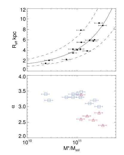
Figure 1.— Top panel: Size-mass relationship for the elliptical galaxy sample. The solid line shows the quadratic model of Hyde & Bernardi (2009) and the dashed lines indicate a scatter of 0.2dex per stellar mass bin. Here, a Chabrier/KTG IMF is adopted. Bottom panel: Tracer power-law density index vs. stellar mass. The red triangles and blue squares indicate GCs and PNe respectively. Higher mass galaxies tend to have tracers with shallower density profiles.

3. Distribution Function

We analyse the dynamical properties of the tracers using a distribution function (henceforth DF) method. DFs are a valuable tool for studying steady state-systems as they replace the impracticality of following individual orbits with a phase-space probability density function. We provide a brief description of these DFs below but direct the interested reader to Evans et al. (1997) and Deason et al. (2011), where more detailed descriptions are given.

For simplicity, we use power-law profiles for the tracer density and potential, namely $\rho\propto r^{-\alpha}$ and $\Phi\propto r^{-\gamma}$, where $\alpha$ and $\gamma$ are constants. Although our formulae hold good for $\gamma\in[-1,1]$, models with $\gamma<0$ are less useful for modelling galaxies. The velocity distribution is given in terms of the binding energy $E=\Phi(r)-\frac{1}{2}(v_{l}^{2}+v_{b}^{2}+v_{\rm los}^{2})$ and the total angular momentum $L=\sqrt{L_{x}^{2}+L_{y}^{2}+L_{z}^{2}}$,

$$F(E,L)\propto L^{-2\beta}f(E)\rho(r)$$ (1)

where

$$f(E)=E^{\beta(\gamma-2)/\gamma+\alpha/\gamma-3/2}$$ (2)

Here, $\beta$ is the Binney anisotropy parameter (Binney 1980), namely

$$\beta=1-\frac{\langle v^{2}_{\theta}\rangle+\langle v^{2}_{\phi}\rangle}{2\langle v^{2}_{r}\rangle},$$ (3)

which is constant for the DFs of form eqn (1).

Our analysis assumes spherical symmetry. While the majority of our elliptical galaxies look spherical in projection (E0/E1) there are a non-negligible number which are more flattened (E6). However, we only consider tracers beyond $2R_{\rm eff}$, well beyond the region from which the galaxy type was inferred. With no prior knowledge of the shape of the potential in these regions, we make the simplest assumption of spherical symmetry. Relaxing this assumption calls for more sophisticated modelling (e.g. de Lorenzi et al. 2007). However, we note that it is not obvious whether this extra complication makes any appreciable difference to the mass estimates (e.g de Lorenzi et al. 2009).

These distribution functions can easily be adapted to probe the rotational properties of the tracers (see Deason et al. 2011). However, in the spherical approximation, it is unphysical for the tracer populations to have substantial rotation. In the limit of mild or no rotation, the mass profile and anisotropy are unaffected by the odd part of the distribution function. To this end, we proceed under the assumption that the tracers are dominated by random rather than systematic motion. In Table 1, we estimate the fractional kinetic energy in rotation, $\left(V_{\rm rot}/\sigma\right)^{2}$, from the kinematic information given in the literature for each sample of tracers (e.g. Table 7 in Coccato et al. 2009). In most cases, this fraction is small ($<20\%$) so it is safe to ignore rotation in our analysis and assume spherical symmetry. However, in a few cases (NGC 4564, NGC 4649 (GC) and NGC 5128 (PNe)), the rotation is quite significant and our assumptions may not be valid. This is most apparent for NGC 4564 where $V_{\rm rot}/\sigma\sim 1$. It is beyond the scope of this paper to model the tracer populations with oblate or triaxial spatial distributions, but we note that excluding these systems from our sample has little difference on our main results.

3.1. Line of sight velocity distribution

In our sample of local galaxies, we do not possess full six-dimensional phase space information for each tracer. However, we can easily marginalise over the unknown components using the DF. We marginalise over the tangential velocity components ($v_{l}$ and $v_{b}$) and line of sight distance ($D$) to obtain the line of sight velocity distribution (LOSVD):

$$F(l,b,v_{\rm los})=\int\int\int F(l,b,D,v_{l},v_{b},v_{\rm los})\,\mathrm{d}v_{l}\,\mathrm{d}v_{b}\,\mathrm{d}D$$ (4)

Here $l$, and $b$ are the Galactocentric longitude and latitude, whilst $v_{\rm los}$ is the line of sight velocity. We assume that all the tracers are bound. Thus, the marginalisation over the tangential velocity components and line of sight distance requires $v_{\rm tot}<v_{\rm esc}$.

This method can be generalized to account for observational errors in the line of sight velocities. We assume the errors are Gaussian and marginalise over the line of sight velocity

$$\bar{F}(l,b,v_{\rm los})=\frac{1}{\sqrt{2\pi\sigma_{\rm los,0}}}\int F(l,b,v_{\rm los})\mathrm{e}^{-\frac{\left(v-v_{los,0}\right)^{2}}{2\sigma_{\rm los,0}^{2}}}\mathrm{d}v_{\rm los}$$ (5)

Here, $v_{\rm los,0}$ is the predicted line of sight velocity and $\sigma_{\rm los,0}$ is the associated error. There are four parameters in our analysis: the potential normalisation ($\Phi_{0}$), the potential power-law slope ($\gamma$), the velocity anisotropy parameter ($\beta$) and the tracer density power-law slope ($\alpha$). We set the tracer density from the power-law approximations made in the previous section. There remains three parameters which we find using a maximum likelihood method. The likelihood function is constructed from the LOSVD

$$\mathrm{log}L(\beta,\Phi_{0},\gamma)=\sum_{i=1}^{N}\mathrm{log}\bar{F}(l_{i},b_{i},,v_{\mathrm{los}_{i}},\beta,\Phi_{0},\gamma),$$ (6)

Eqn (6) gives the three dimensional likelihood as a function of $\beta$, $\gamma$ and $\Phi_{0}$. The total mass within a given radius can then be found from these parameters

$$M(<r)=\frac{\gamma\Phi_{0}}{\mathrm{G}}\left(\frac{r}{\mathrm{kpc}}\right)^{1-\gamma}.$$ (7)

Here, $\Phi_{0}=\Phi(1\rm kpc)$. The analytic mass estimators of Watkins et al. (2010) also assume power-law models for the potential and tracer density. Our analysis extends beyond this formalism as, in addition to an estimate of the total mass, we also constrain the slope of the potential and the velocity anisotropy of the tracers. This is an important improvement as these parameters are often poorly constrained both in theory and observations. Furthermore, by constraining the slope of the potential ($\gamma$), we can report results at a common radius.

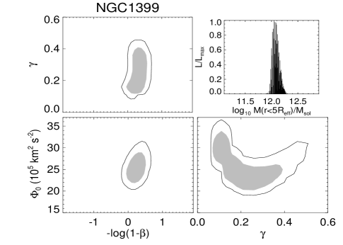
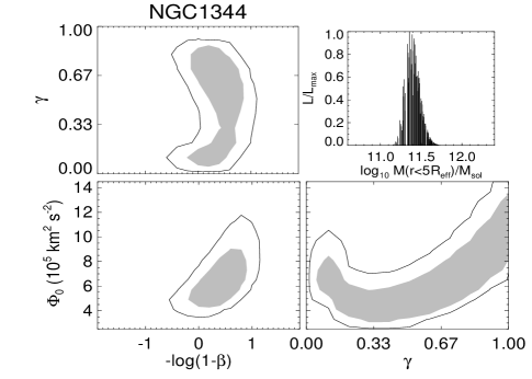
Figure 2.— The maximum likelihood contour levels for NGC 1399 and NGC 1344. The gray shaded regions show the $1\sigma$ (68%) confidence region whilst the black lines encompass the $2\sigma$ (95%) confidence region. The top right panel of each figure shows the likelihood as a function of total mass within $5R_{\rm eff}$.

Name	$R_{\rm max}/R_{\rm eff}$	$\beta$			$\Phi_{0}[10^{5}\mathrm{km}^{2}\mathrm{s}^{-2}]$			$\gamma$
(NGC)		$\bar{\beta}$	$68\%$	$95\%$	$\bar{\Phi}_{0}$	$68\%$	$95\%$	$\bar{\gamma}$	$68\%$	$95\%$
0821	8.1	0.2	[0.1,0.5]	[-0.4,0.6]	7.5	[4.2,9.5]	[3.0,12.2]	0.8	[0.7,1.0]	[0.5,1.0]
1344	6.7	0.3	[0.1,0.5]	[-0.3,0.6]	7.0	[3.5,8.4]	[3.0,11.9]	0.6	[0.4,1.0]	[0.1,1.0]
1399	22.2	0.2	[0.1,0.4]	[-0.1,0.5]	26.0	[21.8,27.5]	[20.7,32.1]	0.2	[0.1,0.3]	[0.1,0.4]
1407	11.7	-0.2	[-0.5,0.2]	[-1.1,0.4]	16.0	[12.3,17.8]	[10.8,21.4]	0.2	[0.1,0.2]	[0.0,0.4]
3377	9.8	0.2	[0.0,0.5]	[-0.4,0.6]	2.6	[1.6,3.2]	[1.2,4.5]	0.3	[0.1,0.3]	[0.0,0.8]
3379	9.2	-0.0	[-0.3,0.3]	[-1.0,0.4]	4.1	[2.7,4.9]	[2.5,6.1]	0.7	[0.5,1.0]	[0.3,1.0]
4374	5.7	0.3	[0.2,0.4]	[-0.1,0.5]	28.8	[17.8,30.8]	[16.5,50.9]	0.3	[0.0,0.3]	[0.0,0.6]
4486	6.0	-1.1	[-1.9,-0.1]	[-4.6,0.3]	42.5	[29.2,48.1]	[26.0,72.4]	0.4	[0.2,0.7]	[0.1,0.8]
4494	7.4	0.1	[-0.2,0.4]	[-0.5,0.5]	3.5	[1.9,3.9]	[1.6,5.7]	0.7	[0.6,1.0]	[0.3,1.0]
4564	10.5	-1.1	[-2.1,0.2]	[-6.4,0.5]	1.6	[0.9,1.7]	[0.8,2.6]	0.7	[0.7,1.0]	[0.1,1.0]
4636	8.6	0.2	[0.0,0.5]	[-0.4,0.7]	15.8	[9.5,17.8]	[8.3,26.3]	0.4	[0.1,0.5]	[0.0,0.7]
4649 (GC)	5.3	-0.7	[-1.5,0.2]	[-3.4,0.6]	14.0	[7.2,15.8]	[6.2,31.6]	0.5	[0.1,0.7]	[0.1,0.9]
4649 (PNe)	4.1	0.1	[-0.2,0.4]	[-0.6,0.5]	18.0	[6.9,21.7]	[6.5,33.5]	0.6	[0.6,1.0]	[0.0,1.0]
4697	5.2	-0.5	[-1.0,-0.1]	[-1.5,0.1]	4.0	[2.5,4.4]	[2.3,6.0]	0.7	[0.6,1.0]	[0.2,1.0]
5128 (GC)	5.4	0.2	[-0.1,0.4]	[-0.4,0.5]	9.2	[6.2,10.4]	[5.3,13.4]	0.4	[0.1,0.5]	[0.0,0.8]
5128 (PNe)	15.6	0.5	[0.4,0.6]	[0.3,0.7]	10.7	[6.1,12.6]	[5.0,16.8]	0.7	[0.6,0.9]	[0.4,1.0]
5846	3.9	0.2	[0.0,0.5]	[-0.7,0.7]	23.8	[8.2,28.1]	[6.8,53.2]	0.6	[0.6,1.0]	[0.1,1.0]

Table 2Likelihood parameters. We give the galaxy name and maximum projected radius (scaled by effective radius) in the first two columns. The remaining columns give the weighted mean of the velocity anisotropy, potential normalisation and potential power-law slope with their 68% and 95% confidence intervals.

4. Results

We summarise the maximum likelihood parameters in Table 2. In Fig. 2, we show the likelihood contours for NGC 1399 and NGC 1344 as examples. The grey shaded region shows the $68\%$ confidence boundary and the solid line gives the $95\%$ confidence boundary. Note that each panel shows a 2D slice of the likelihood values. There is a strong degeneracy between the potential normalisation and power-law slope (note the ‘banana’ shape in the bottom right-hand panels). While we do not strongly constrain these individual parameters, the mass profile is better defined as shown in the top right hand panels of Fig. 2.

First, we compare our results to the analytic mass estimators described in Watkins et al. (2010). These mass estimators compute the mass within the maximum 3D radius of the tracers, $r_{\rm max}$. For a spherical distribution of stars with density distribution $\rho$, the average 3D radius of a star with projected radius, R is given by:

$$\langle r\rangle=\frac{\int_{-\infty}^{\infty}r\,\rho(R,z)\,dz}{\int_{-\infty}^{\infty}\rho(R,z)\,dz}$$ (8)

For a power-law distribution of tracers, this equation is analytic and can be expressed as

$$\langle r\rangle=\frac{\Gamma[\alpha/2]\Gamma[\alpha/2-1]}{\left(\Gamma[\alpha/2-1/2]\right)^{2}}\,R$$ (9)

Here, $\alpha$ is the power-law index of the tracer density profile. Using equations 26 and 27 from Watkins et al. (2010), we estimate the mass using the maximum likelihood $\gamma$ and $\beta$ values. We also evaluate the mass assuming an isothermal potential ($\gamma=0$) or Keplerian potential ($\gamma=1$) with isotropic orbits ($\beta=0$). These values are compared to our maximum likelihood mass within $\langle r_{\rm max}\rangle$ (see eqn 7) in Fig. 3.

We see very good agreement between our estimated masses and those of Watkins et al. (2010) when the potential slope and anisotropy are given. The agreement is within $\sim 10\%$ for all the systems. However, when an isothermal potential (blue) or Keplerian potential (red) with isotropic tracers is assumed, there can be quite large discrepancies. The mass is systematically overestimated when an isothermal potential is assumed. In this case, the discrepancies can be as large as $100\%$. Conversely, if we had adopted a Keplerian potential the mass would be systematically underestimated. The disagreement is worsened for systems where the velocity anisotropy deviates from isotropy and/or the potential is not close to isothermal or Keplerian. These findings illustrate the effectiveness of our technique to estimate masses, as we make no strong assumptions about the velocity anisotropy or potential power-law slope.

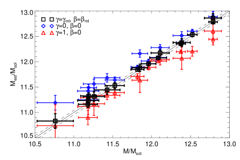
Figure 3.— Comparison with the mass estimator of Watkins et al. (2010). We show the agreement between our masses within $r_{\rm max}$ ($M(r<r_{\rm max})$) and the estimated masses from the Watkins et al. (2010) formalism ($M_{\rm est}$). The black squares show the Watkins et al. (2010) mass estimates given our maximum likelihood $\beta$ and $\gamma$. The red triangles and blue diamonds show the mass estimators assuming velocity isotropy ($\beta=0$) with a Keplerian potential ($\gamma=1$) and an isothermal potential ($\gamma=0$) respectively. The solid line shows a one-to-one relation, and the dashed lines show 10% discrepancies.

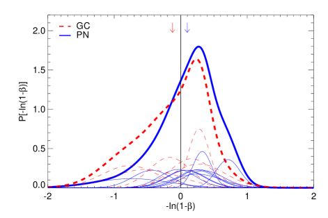
Figure 4.— The velocity anisotropy distributions for the globular clusters (red dashed lines) and PNe (blue solid lines). The thick lines show the sum of the Gaussian kernels for each measurement. Individual contributions are shown with the thinner lines. In general, the PNe orbits are isotropic/mildly radially biased whilst the globular cluster orbits are isotropic/mildly tangential.

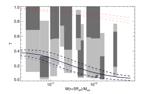
Figure 5.— The slope of the overall power-law potential ($\Phi\propto r^{-\gamma}$) vs. the total mass enclosed within 5 effective radii. The dark and light gray bands show the 68% and 95% confidence regions respectively. The solid black, dot-dashed blue and dotted red lines give the model predictions (within $10-100$kpc) for bulge+halo, halo and bulge models respectively.

In Fig. 4, we show the velocity anisotropy distributions of the globular cluster tracers (red lines) and PNe tracers (blue lines). Each measurement is described by a Gaussian centred on the estimated value with a dispersion given by the predicted ($1\sigma$) error. These Gaussian kernels are then summed to produce an overall distribution which is shown by the thick lines. Individual contributions are shown with the thinner lines. The PNe are generally more radially biased than the globular clusters. This has been noted by previous authors who find that GCs generally have mildly tangential/isotropic orbits whilst PNe tend to have mildly radial/isotropic orbits (e.g. Hwang et al. 2008; Romanowsky et al. 2009; Woodley et al. 2010; Napolitano et al. 2011). Note that the most tangentially biased PNe system belongs to NGC 4564 which, as noted in the previous section, has evidence for substantial rotation.

The slope of the overall power-law potential ($\Phi\propto r^{-\gamma}$) is shown in Fig. 5 as a function of total mass within five effective radii. The black points give the weighted mean $\gamma$ values and the dark and light gray bands show the 68% and 95% confidence regions respectively. The solid and dashed lines give model predictions for the power-law slope with their associated scatter. These models are described in more detail in Section 4.1.1. The black lines show the slope-mass relation for bulge+halo models where a Hernquist profile is assumed for the stellar component and a Navarro-Frenk-White profile is assumed for the dark matter component. The red and blue lines show the relation with only a stellar or dark matter component respectively. The slopes for these models are computed between $10-100$ kpc.

At present, our $\gamma$ values are too poorly constrained to distinguish between different model profiles. In the 95% confidence interval the slopes lie in between an isothermal ($\gamma=0$) and Keplerian ($\gamma=1$) regime. However, there is tentative evidence for a trend with galaxy mass – namely, the less massive galaxies have steeper potential profiles than the more massive galaxies. This trend is clear in the models, but is less so in the data. We tested the (anti)-correlation of $\gamma$ with mass in the data using a Spearman rank test. Given the probability distribution of $\gamma$ values (derived from the marginalised likelihood distributions), we draw a $\gamma$ value at random for each galaxy. The correlation with mass is then tested with a Spearman rank statistic. The exercise is repeated for $10^{5}$ trials. We find that only $20\%$ of the trials have a $95\%$ significant trend. This exercise suggests that it is premature to claim an (anti)-correlation between potential slope and mass from the current constraints. We note that Barnabè et al. (2011) also find a tentative indication that less massive galaxies have steepr potential slopes.

Auger et al. (2010a) and Koopmans et al. (2009) find almost isothermal profiles for the SLACS elliptical galaxy sample within $1R_{\rm eff}$. The SLACS sample is biased towards the more massive galaxies where isothermal models are also predicted by the bulge+halo models.

4.1. Dark matter fractions

The maximum likelihood normalisation (i.e. total mass) and power-law slope define the overall potential. To separate the dark matter and baryonic components, we assume the stars follow a Hernquist profile (Hernquist 1990). To convert luminosity into stellar mass, we assume either a Chabrier/KTG (Chabrier 2003; Kroupa et al. 1993) IMF with $(M/L_{B})^{*}=3.5-5.5$ or a Salpeter (Salpeter 1955) IMF with $(M/L_{B})^{*}=6-10$ (e.g. Gerhard et al. 2001; Tortora et al. 2009). We assume the stellar mass-to-light ratios cover the given range with a flat prior, so all values in the range have equal weight. This range is taken into account in the estimated error of the stellar mass (see Table 3). The fraction of dark matter within a certain radius is given by

$$f_{\rm DM}(<r)=1-M^{*}(<r)/M_{\rm tot}(<r).$$ (10)

Here, we have have assumed that the gas mass is negligible relative to the stellar mass. As we are considering radial scales of $\sim 0.1r_{\rm vir}$ this is a good approximation (e.g. O’Sullivan et al. 2007).

In recent years, the fraction of dark matter as a function of galaxy mass has been studied extensively in the literature (e.g. Padmanabhan et al. 2004; Cardone et al. 2009; Tortora et al. 2009; Cardone & Tortora 2010; Auger et al. 2010a; Grillo 2010; Barnabè et al. 2011). Most of these studies have been limited to within one effective radius. Here, we concentrate on the fraction of dark matter within five effective radii - a region relatively unexplored in local elliptical galaxies.

4.1.1 Models

Name	$M(<5R_{\rm eff})$	$M/L_{B}$	IMF	$M^{*}$	$f_{\rm DM}$
(NGC)	[$10^{11}M_{\odot}]$	$(<5R_{\rm eff})$		[$10^{11}M_{\odot}]$	$(<5R_{\rm eff})$
0821	2.3 $\pm$ 0.6	8 $\pm$ 2	C	1.2 $\pm$ 0.2	0.59 $\pm$ 0.11
			S	2.1 $\pm$ 0.4	0.27 $\pm$ 0.20
1344	2.6 $\pm$ 0.5	14 $\pm$ 2	C	0.8 $\pm$ 0.2	0.74 $\pm$ 0.05
			S	1.5 $\pm$ 0.3	0.54 $\pm$ 0.10
1399	12.5 $\pm$ 1.8	35 $\pm$ 5	C	1.6 $\pm$ 0.3	0.90 $\pm$ 0.02
			S	2.8 $\pm$ 0.5	0.82 $\pm$ 0.03
1407	9.4 $\pm$ 1.3	19 $\pm$ 2	C	2.1 $\pm$ 0.4	0.82 $\pm$ 0.03
			S	3.8 $\pm$ 0.7	0.67 $\pm$ 0.05
3377	0.7 $\pm$ 0.2	12 $\pm$ 2	C	0.3 $\pm$ 0.0	0.70 $\pm$ 0.07
			S	0.5 $\pm$ 0.1	0.46 $\pm$ 0.13
3379	1.3 $\pm$ 0.2	9 $\pm$ 1	C	0.6 $\pm$ 0.1	0.61 $\pm$ 0.07
			S	1.1 $\pm$ 0.2	0.31 $\pm$ 0.12
4374	15.9 $\pm$ 1.9	31 $\pm$ 3	C	2.2 $\pm$ 0.4	0.89 $\pm$ 0.01
			S	4.0 $\pm$ 0.7	0.80 $\pm$ 0.02
4486	31.7 $\pm$ 3.2	43 $\pm$ 4	C	3.3 $\pm$ 0.6	0.92 $\pm$ 0.01
			S	5.8 $\pm$ 1.0	0.85 $\pm$ 0.02
4494	1.2 $\pm$ 0.2	5 $\pm$ 1	C	1.0 $\pm$ 0.2	0.32 $\pm$ 0.12
			S	1.8 $\pm$ 0.3	-0.21 $\pm$ 0.22
4564	0.4 $\pm$ 0.1	7 $\pm$ 2	C	0.2 $\pm$ 0.0	0.54 $\pm$ 0.17
			S	0.4 $\pm$ 0.1	0.18 $\pm$ 0.30
4636	10.8 $\pm$ 1.9	40 $\pm$ 6	C	1.2 $\pm$ 0.2	0.91 $\pm$ 0.02
			S	2.1 $\pm$ 0.4	0.84 $\pm$ 0.03
4649	8.8 $\pm$ 1.3	14 $\pm$ 2	C	2.8 $\pm$ 0.5	0.74 $\pm$ 0.04
			S	4.9 $\pm$ 0.9	0.54 $\pm$ 0.07
4697	1.4 $\pm$ 0.2	7 $\pm$ 1	C	0.8 $\pm$ 0.2	0.51 $\pm$ 0.08
			S	1.5 $\pm$ 0.3	0.12 $\pm$ 0.13
5128	4.7 $\pm$ 0.5	17 $\pm$ 1	C	1.2 $\pm$ 0.2	0.79 $\pm$ 0.02
			S	2.2 $\pm$ 0.4	0.63 $\pm$ 0.04
5846	11.3 $\pm$ 2.7	28 $\pm$ 6	C	1.8 $\pm$ 0.3	0.87 $\pm$ 0.03
			S	3.2 $\pm$ 0.6	0.77 $\pm$ 0.05

Table 3Dark matter fraction parameters. We give the galaxy name, total mass-to-light ratio within $5R_{\rm eff}$, adopted IMF (Chabrier/KTG (C) or Salpeter (S)), stellar mass and fraction of dark matter within $5R_{\rm eff}$.

Before proceeding, we construct some simple models to show the expected relation between dark matter fraction (within a certain radius) and galaxy mass. We apply the following steps:

• Abundance matching is used to relate the halo mass ($M_{200}$) to the stellar mass. We use the prescription given by Behroozi et al. (2010). The stellar mass-halo mass relation is given by their Equation (21) with parameters listed in Table (2). These authors adopt a $\Lambda$CDM cosmology using the WMAP5 parameters. The scatter in stellar mass for a given halo mass is $\sim 0.15$ dex. This abundance matching is applicable for a Chabrier/KTG IMF. To convert to a Salpeter IMF, the stellar masses are increased by a factor of 0.25 dex.

• An NFW profile is adopted to model the density profile of the halo. This profile is fully described by two parameters: the halo mass and concentration. We relate the concentration to the halo mass using the relation given in Macciò et al. (2008) for WMAP5. At this stage, we have a fully defined dark matter profile for a particular stellar mass. The scatter in this relation for a given halo mass is $\sim 0.1$ dex.

• Using the quadratic size-mass relation given in Hyde & Bernardi (2009) based on SDSS data, we calculate the effective radius of a galaxy from the stellar mass. The scatter for a given stellar mass is $\sim 0.2$ dex. The form of this size-mass relation is shown in the top panel of Fig, 1 against the observed values in our sample.

• Finally, we adopt a Hernquist profile for the stellar profile which is defined from the total stellar mass and effective radius.

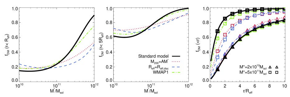
Figure 6.— The dark matter fraction within one (left panel) and five (middle panel) effective radii as a function of stellar mass. The solid black line is our adopted model. The dotted red line shows the relation when a linear stellar mass-halo mass relation is used $M_{200}=AM^{*}$. The dashed blue line shows a model with a size-mass relationship applicable to disc galaxies. The dot-dashed green line shows the model prediction when a WMAP1 cosmology is adopted. In the right-hand panel we show the dark matter fraction as a function of radius (scaled by $R_{\rm eff}$) for the different models. The triangle and square symbols show the profiles for lower ($M^{*}\sim 2\times 10^{10}M_{\odot}$) and higher ($M^{*}\sim 5\times 10^{11}M_{\odot}$) mass galaxies respectively.

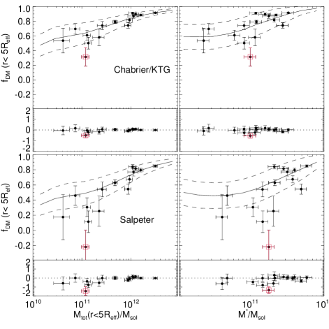
Figure 7.— The dark matter fraction ratio within 5 effective radii vs. total mass within 5 effective radii (left) and stellar mass (right). A Chabrier/KTG ($(M/L)^{*}\sim 4.5$) and Salpeter ($(M/L)^{*}\sim 8$) IMF is assumed in the top and bottom panels respectively. The solid line indicates the predicted relation from simulations. The predicted scatter is given by the dashed lines. The inset panels show the residuals of the data vs. models. The red square highlights NGC 4494 which is inconsistent with stellar mass-to-light ratios larger than $(M/L)^{*}\sim 5$.

We now have a dark matter and stellar profile defined for any particular stellar mass. In addition, we take into account the scatter introduced in each step of the analysis. These are propagated forward using Monte Carlo techniques. We emphasize that there are no free parameters in these models that need to be fitted to the data.

The models predict an increase in dark matter fraction within 5 $R_{\rm eff}$ with increasing total/stellar mass (see black line in Fig. 6). This general trend is independent of the IMF used. The fraction of dark matter within a scaled number of effective radii is driven by two factors: the star formation efficiency and the concentration of these stars within the dark matter halo (cf. Zaritsky et al. 2008).

The star formation efficiency is implemented in the models from the stellar mass-halo mass relation. The abundance matching, by construction, reproduces the observable stellar mass function. It is well known that there is a universal U-shaped trend of star formation efficiency (e.g. Benson et al. 2000; Marinoni & Hudson 2002; Napolitano et al. 2005; van den Bosch et al. 2007; Conroy & Wechsler 2009). The peak efficiency occurs at $M^{*}\sim 10^{11}$ where increasingly massive galaxies have a lower efficiency due to the large cooling time of their hot gas (e.g. White & Rees 1978) and the least massive systems are unable to retain their primordial gas content for long enough to form stars. Hence, the the lowest mass and highest mass galaxies are the most dark matter dominated.

The second factor driving the trend of dark matter fractions is the size-mass relationship of early type galaxies. With increasing total (or stellar) mass the effective radius increases (see Fig. 1). In addition, the size increases more steeply with increasing mass. This ‘baryon un-packing’ is an important factor when we are considering the dark matter content within a scaled number of effective radii. Regardless of the dark matter halo properties (or star formation efficiency), a higher concentration of baryons (or smaller effective radius) leads to smaller dark matter fractions. This simple scaling behaviour has been noted by previous authors (e.g. Padmanabhan et al. 2004; Tortora et al. 2009; Napolitano et al. 2010; Dutton et al. 2011). Note that disc galaxies have a much shallower size-mass relation. Thus, the dark matter fractions are approximately constant with mass for these galaxies (e.g. Dutton et al. 2011).

In Fig. 6, we illustrate the dependence of our model on the adopted stellar mass-halo mass relation, size-mass relation and cosmology. The solid black lines indicate our adopted model. We consider three variations to our adopted model (shown by the coloured dotted, dashed and dot-dashed lines):

• Stellar mass-halo mass relation: We adopt a linear relation of the form $M_{200}=AM^{*}$. The normalisation constant is set using the mean halo mass corresponding to a stellar mass of $M^{*}\sim 10^{11}$ from our original abundance matching relation. Models adopting this relation are shown with the red lines.

• Size-mass relation: We consider a size-mass relation applicable to disc galaxies. This is derived using the Pizagno et al. (2007) sample of disc galaxies. The stellar masses are derived from the colours according to the prescription of Bell et al. (2003). A -0.15dex offset was applied to provide stellar masses consistent with a Chabrier/KTG IMF. We then fit a linear relation between effective radius and stellar mass to approximate a size-mass relationship. Models assuming this size-mass relation are shown by the blue lines.

• Cosmology: We adopt a WMAP1 cosmology instead of the more recent WMAP5 parameters. In this case the stellar mass-halo mass relation is taken from Guo et al. (2010) (who adopt a WMAP1 cosmology) and the WMAP1 mass concentration relation is used from Macciò et al. (2008). This is shown by the green lines.

The purpose of these variations is to emphasize the key ingredients in our adopted model driving the apparent trend. Thus, these variations are for illustrative purposes only and we are not proposing that they are viable alternatives to our adopted model. For example, adopting a size-mass relation applicable to disc galaxies is a particularly poor assumption when applied to elliptical galaxies.

The left and middle panels show the dark matter fraction within one and five effective radii as a function of stellar mass. We have not included the scatter, so this figure only illustrates the mean dependence of the models. Note that a Chabrier/KTG IMF is assumed but the same trends are seen with a Salpeter IMF. Adopting a different cosmology only slightly affects the dark matter fraction-stellar mass relation. As alluded to earlier, the relationship is driven by star formation efficiency and baryon extent. By adopting a shallower size-mass relation (applicable to disc galaxies) the dark matter fractions are constant over a large range of stellar mass. A similar effect is seen by allowing for a linear stellar mass-halo mass relation. The effects are the most severe within one effective radii as the baryons are more dominant at smaller radii.

In the right-hand panel, we show the dark matter fraction as a function of radius (scaled by $R_{\rm eff}$). The profiles of the higher mass galaxies ($M^{*}\sim 5\times 10^{11}M_{\odot}$) are more model dependent than those of lower mass galaxies ($M^{*}\sim 2\times 10^{10}M_{\odot}$).

4.1.2 Comparison with data

In Fig. 7, we show the dark matter fractions within five effective radii as a function of total mass within this radius (left) and as a function of total stellar mass (right). The top panels show the relation for a Chabrier/KTG IMF and bottom panels are for a Salpeter IMF. The symbols with error bars are the data points derived in this work and the solid and dashed lines give the predicted relation from the models with the associated ($1\sigma$) scatter. The residuals of the data vs. model (i.e. (data-model)/model) are shown in the inset panels.

In general, the model is in good agreement with the data when a Chabrier/KTG IMF is adopted. Our dark matter fractions are in good agreement with previous studies which find $f_{\rm DM}(<5R_{\rm eff})\sim 0.4-0.5$ for ordinary ellipticals (e.g. NGC 4494, NGC 3379, NGC 4697 see Figure 12 in Napolitano et al. 2011) and $f_{\rm DM}(<5R_{\rm eff})\sim 0.8-0.9$ for group or cluster central ellipticals (e.g. NGC 1399, NGC 1407, NGC 4486, NGC 4648, NGC 5846 see Figure 8 in Das et al. 2010).

Note that our total mass estimates (given within $5R_{\rm eff}$ in Table 3), and hence dark matter fractions, usually have smaller uncertainties than those found in more general dynamical modelling (e.g. de Lorenzi et al. 2007; de Lorenzi et al. 2009). This is because such numerical modelling procedures allow for more general solutions (e.g. non-constant anisotropy, triaxiality) and thus cover a larger parameter space. Nonetheless, our simplistic approach is much more easily applied to a large sample of galaxies and hence this work is complementary to more general numerical methods.

The red square highlighted is NGC 4494, which has a curiously low dark matter fraction. Napolitano et al. (2009) studied this system in detail and found an abnormally low dark matter concentration and also derive a similar dark matter fraction within 5$R_{\rm eff}$. The remaining low mass galaxies have dark matter fractions consistent with the model predictions (at least for a Chabrier/KTG IMF). While the case of NGC 4494 is in contradiction to the predictions from simulations, the general trend suggests that the dark matter properties of lower mass galaxies are not very different from those of higher masses. However, a larger sample of tracers, probing both low and high masses, is needed to investigate this further.

Adopting a Salpeter IMF causes some of the low mass systems to have lower than predicted dark matter fractions. On the other hand, a Chabrier/KTG IMF is able to describe the trend over a wide range of masses. A secondary factor that may influence the dark matter fraction-mass relation is variations in stellar population properties, such as a non-universal IMF (e.g Auger et al. 2010b; Treu et al. 2010). We find no evidence for a variation in IMF with mass from Fig. 7. The suggested IMF variation, where the stellar-mass to light ratio increases with mass, would require the fraction of dark matter to increase more steeply when a universal IMF is adopted. However, we are probing out to five effective radii, well beyond the regions where the baryonic material is dominant so are less sensitive to IMF variations than studies probing within one effective radii. We compare our models with such studies in the following section.

Figure 8.— The projected dark matter fraction ratio within 0.5 effective radii vs. total mass within 0.5 effective radii (left) and stellar mass (right). The data points are for the SLACS sample of elliptical galaxies published in Auger et al. (2010a). The inset panels show the residuals of the data vs. model.

4.1.3 Comparison with SLACS data

In Fig. 8, we show the projected dark matter fractions as a function of galaxy mass and stellar mass. The data points derive from the SLACS sample of Auger et al. (2010a). This work focuses on relatively high mass galaxies within one effective radius. The simple models that we employ here are able to explain the overall trend of increasing dark matter fraction with galaxy mass. Similar to the case at larger radii, adopting a Salpeter IMF leads to lower dark matter fractions than the model predictions. In fact, several systems are consistent with a negative dark matter fraction, which suggests that adopting a Salpeter IMF for such systems is unphysical. Once again a universal Chabrier/KTG IMF is able to explain the dark matter fraction-mass relation reasonably well. Variations in IMF with mass can in principle be probed by deviations of the data from the model predictions. Qualitatively, we see no evidence for a difference in slope between the data and the model. However, a more sophisticated model is required to investigate these variations in detail. In summary, we find that the variation in dark matter fraction with galaxy mass is consistent with a simple, universal IMF halo model.

Recently, Grillo (2010) finds a constant, if not decreasing, projected dark matter fraction with galaxy mass. This is inconsistent with both our models and our measurements as well as with the measurements by Auger et al. (2010a), independently of the adopted IMF. Grillo (2010) suggests that these contrasting results may be due to other studies being more model dependent (e.g. Padmanabhan et al. 2004; Tortora et al. 2009 who give three dimensional dark matter fractions) and/or the more massive early type galaxy bias of their sample. However, this is difficult to reconcile with the results of Auger et al. (2010a) who also give projected dark matter fractions (i.e. with minimal modelling assumptions) and have a similar mass bias in their sample.

5. Conclusions

We studied the mass profiles of local elliptical galaxies using planetary nebulae (PNe) and globular clusters (GCs) as distant tracers (with $R>2R_{\rm eff}$). A sample of 15 galaxies was compiled from the literature. A distribution function-maximum likelihood method was used to study the dynamics of the tracers under the assumptions of spherical symmetry and power-law models for the (overall) potential and tracer density. We summarise our conclusions as follows:

(1) We compared our distribution function-maximum likelihood method to the analytic mass estimators of Watkins et al. (2010). There is good agreement when we adopt our maximum likelihood velocity anisotropy and potential power-law indices into the Watkins et al. (2010) formalism. However, assuming isotropy and an isothermal/Keplerian potential leads to a systematic overestimate/underestimate of the mass (by up to $\sim 100\%$). Our method makes no strong assumptions about the values of the velocity anisotropy and potential power-law slope. This is an important improvement, as these parameters are difficult to constrain by other means.

(2) The PNe are generally more centrally concentrated (following closely the stellar luminosity, see Coccato et al. 2009) and are on more radial orbits than the GCs. This may be related to the parent galaxy properties as the PNe tend to trace the less massive systems, but could also reflect differences between the GC and PNe populations (e.g. GCs are generally older).

(3) The slope of the overall (power-law) potential is not strongly constrained but lies in between the isothermal ($\gamma=0$) and Keplerian ($\gamma=1$) regimes. In the models the less massive galaxies have steeper potential profiles than those of the more massive galaxies. There is tentative evidence that this trend is also present in the data. However, a Monte Carlo test using the Spearman rank statistic shows no evidence for a clear trend. Recently, Koopmans et al. (2009) and Auger et al. (2010a) found roughly isothermal density profiles for their sample of (massive) elliptical galaxies within an effective radius. This is in good agreement with bulge+halo models for the more massive elliptical galaxies.

(4) We constructed simple halo models to predict the expected relation between dark matter fraction and halo mass. The combination of star formation efficiency (stellar mass-halo mass relation) and baryon concentration (size-mass relation) is able to describe the observed trend of increasing dark matter fraction within a scaled number of effective radii. We find no evidence for an additional factor, such as a non-universal IMF, affecting this relation. The dark matter fractions are consistent with the models when a universal Chabrier/KTG IMF is assumed for elliptical galaxies. In particular, a Salpeter IMF is inconsistent with some of the lower mass galaxies. This is in good agreement with Cappellari et al. (2006) who reached the same conclusion using a completely different approach.

Finally, let us remark that we have neglected the influence of baryonic processes on the distribution of dark matter. Our adopted NFW profile is applicable for a ‘pristine’ dark matter distribution, un-modified by the process of galaxy formation. For example, collapsing gas can exert a gravitational drag on the dark matter leading to a more concentrated dark matter halo (i.e. Blumenthal et al. 1986; Gnedin et al. 2004). On the other hand, rapid supernova driven feedback processes can drive the dark matter particles away from the centre of the galaxy (e.g. Pontzen & Governato 2011) leading to halo expansion. Halo contraction or expansion can increase or decrease the fraction of dark matter within a given radius. The importance of these processes is poorly understood and we make not attempt to model them in this work. However, we note that this is another secondary effect (in addition to IMF variations) that should be explored with more sophisticated modelling.

References

- Auger et al. (2010a) Auger, M. W., Treu, T., Bolton, A. S., Gavazzi, R., Koopmans, L. V. E., Marshall, P. J., Moustakas, L. A., & Burles, S. 2010a, ApJ, 724, 511
- Auger et al. (2010b) Auger, M. W., Treu, T., Gavazzi, R., Bolton, A. S., Koopmans, L. V. E., & Marshall, P. J. 2010b, ApJ, 721, L163
- Barnabè et al. (2011) Barnabè, M., Czoske, O., Koopmans, L. V. E., Treu, T., & Bolton, A. S. 2011, MNRAS, 415, 2215
- Behroozi et al. (2010) Behroozi, P. S., Conroy, C., & Wechsler, R. H. 2010, ApJ, 717, 379
- Bell et al. (2003) Bell, E. F., McIntosh, D. H., Katz, N., & Weinberg, M. D. 2003, ApJS, 149, 289
- Benson et al. (2000) Benson, A. J., Cole, S., Frenk, C. S., Baugh, C. M., & Lacey, C. G. 2000, MNRAS, 311, 793
- Binney (1980) Binney, J. 1980, MNRAS, 190, 873
- Blumenthal et al. (1986) Blumenthal, G. R., Faber, S. M., Flores, R., & Primack, J. R. 1986, ApJ, 301, 27
- Cappellari et al. (2006) Cappellari, M., et al. 2006, MNRAS, 366, 1126
- Cardone & Tortora (2010) Cardone, V. F., & Tortora, C. 2010, MNRAS, 409, 1570
- Cardone et al. (2009) Cardone, V. F., Tortora, C., Molinaro, R., & Salzano, V. 2009, A&A, 504, 769
- Chabrier (2003) Chabrier, G. 2003, PASP, 115, 763
- Ciotti (1991) Ciotti, L. 1991, A&A, 249, 99
- Coccato et al. (2009) Coccato, L., et al. 2009, MNRAS, 394, 1249
- Conroy & Wechsler (2009) Conroy, C., & Wechsler, R. H. 2009, ApJ, 696, 620
- Côté et al. (2001) Côté, P., et al. 2001, ApJ, 559, 828
- Das et al. (2010) Das, P., Gerhard, O., Churazov, E., & Zhuravleva, I. 2010, MNRAS, 409, 1362
- de Lorenzi et al. (2007) de Lorenzi, F., Debattista, V. P., Gerhard, O., & Sambhus, N. 2007, MNRAS, 376, 71
- de Lorenzi et al. (2008) de Lorenzi, F., Gerhard, O., Saglia, R. P., Sambhus, N., Debattista, V. P., Pannella, M., & Méndez, R. H. 2008, MNRAS, 385, 1729
- de Lorenzi et al. (2009) de Lorenzi, F., et al. 2009, MNRAS, 395, 76
- de Vaucouleurs et al. (1991) de Vaucouleurs, G., de Vaucouleurs, A., Corwin, Jr., H. G., Buta, R. J., Paturel, G., & Fouque, P. 1991, Third Reference Catalogue of Bright Galaxies (Springer-Verlag Berlin Heidelberg New York)
- Deason et al. (2011) Deason, A. J., Belokurov, V., & Evans, N. W. 2011, MNRAS, 411, 1480
- Dekel et al. (2005) Dekel, A., Stoehr, F., Mamon, G. A., Cox, T. J., Novak, G. S., & Primack, J. R. 2005, Nature, 437, 707
- Dirsch et al. (2005) Dirsch, B., Schuberth, Y., & Richtler, T. 2005, A&A, 433, 43
- Douglas et al. (2002) Douglas, N. G., et al. 2002, PASP, 114, 1234
- Douglas et al. (2007) —. 2007, ApJ, 664, 257
- Dutton et al. (2011) Dutton, A. A., et al. 2011, MNRAS, 416, 322
- Evans et al. (1997) Evans, N. W., Hafner, R. M., & de Zeeuw, P. T. 1997, MNRAS, 286, 315
- Faure et al. (2011) Faure, C., et al. 2011, A&A, 529, A72+
- Forbes et al. (2006) Forbes, D. A., Sánchez-Blázquez, P., Phan, A. T. T., Brodie, J. P., Strader, J., & Spitler, L. 2006, MNRAS, 366, 1230
- Gavazzi et al. (2007) Gavazzi, R., Treu, T., Rhodes, J. D., Koopmans, L. V. E., Bolton, A. S., Burles, S., Massey, R. J., & Moustakas, L. A. 2007, ApJ, 667, 176
- Gerhard et al. (2001) Gerhard, O., Kronawitter, A., Saglia, R. P., & Bender, R. 2001, AJ, 121, 1936
- Gnedin et al. (2004) Gnedin, O. Y., Kravtsov, A. V., Klypin, A. A., & Nagai, D. 2004, ApJ, 616, 16
- Grillo (2010) Grillo, C. 2010, ApJ, 722, 779
- Guo et al. (2010) Guo, Q., White, S., Li, C., & Boylan-Kolchin, M. 2010, MNRAS, 404, 1111
- Hernquist (1990) Hernquist, L. 1990, ApJ, 356, 359
- Humphrey et al. (2006) Humphrey, P. J., Buote, D. A., Gastaldello, F., Zappacosta, L., Bullock, J. S., Brighenti, F., & Mathews, W. G. 2006, ApJ, 646, 899
- Hwang et al. (2008) Hwang, H. S., et al. 2008, ApJ, 674, 869
- Hyde & Bernardi (2009) Hyde, J. B., & Bernardi, M. 2009, MNRAS, 394, 1978
- Johnson et al. (2009) Johnson, R., Chakrabarty, D., O’Sullivan, E., & Raychaudhury, S. 2009, ApJ, 706, 980
- Koopmans et al. (2009) Koopmans, L. V. E., et al. 2009, ApJ, 703, L51
- Kroupa et al. (1993) Kroupa, P., Tout, C. A., & Gilmore, G. 1993, MNRAS, 262, 545
- Lee et al. (2008) Lee, M. G., et al. 2008, ApJ, 674, 857
- Leier et al. (2011) Leier, D., Ferreras, I., Saha, P., & Falco, E. E. 2011, ArXiv e-prints
- Loewenstein & White (1999) Loewenstein, M., & White, III, R. E. 1999, ApJ, 518, 50
- Macciò et al. (2008) Macciò, A. V., Dutton, A. A., & van den Bosch, F. C. 2008, MNRAS, 391, 1940
- Mamon & Łokas (2005) Mamon, G. A., & Łokas, E. L. 2005, MNRAS, 363, 705
- Marinoni & Hudson (2002) Marinoni, C., & Hudson, M. J. 2002, ApJ, 569, 101
- Mei et al. (2007) Mei, S., et al. 2007, ApJ, 655, 144
- Méndez et al. (2009) Méndez, R. H., Teodorescu, A. M., Kudritzki, R.-P., & Burkert, A. 2009, ApJ, 691, 228
- Napolitano et al. (2010) Napolitano, N. R., Romanowsky, A. J., & Tortora, C. 2010, MNRAS, 405, 2351
- Napolitano et al. (2005) Napolitano, N. R., et al. 2005, MNRAS, 357, 691
- Napolitano et al. (2009) —. 2009, MNRAS, 393, 329
- Napolitano et al. (2011) —. 2011, MNRAS, 411, 2035
- O’Sullivan & Ponman (2004) O’Sullivan, E., & Ponman, T. J. 2004, MNRAS, 354, 935
- O’Sullivan et al. (2007) O’Sullivan, E., Sanderson, A. J. R., & Ponman, T. J. 2007, MNRAS, 380, 1409
- Padmanabhan et al. (2004) Padmanabhan, N., et al. 2004, New A, 9, 329
- Peng et al. (2004) Peng, E. W., Ford, H. C., & Freeman, K. C. 2004, ApJ, 602, 705
- Pizagno et al. (2007) Pizagno, J., et al. 2007, AJ, 134, 945
- Pontzen & Governato (2011) Pontzen, A., & Governato, F. 2011, ArXiv e-prints
- Romanowsky et al. (2003) Romanowsky, A. J., Douglas, N. G., Arnaboldi, M., Kuijken, K., Merrifield, M. R., Napolitano, N. R., Capaccioli, M., & Freeman, K. C. 2003, Science, 301, 1696
- Romanowsky et al. (2009) Romanowsky, A. J., Strader, J., Spitler, L. R., Johnson, R., Brodie, J. P., Forbes, D. A., & Ponman, T. 2009, AJ, 137, 4956
- Rusin & Kochanek (2005) Rusin, D., & Kochanek, C. S. 2005, ApJ, 623, 666
- Saglia et al. (2000) Saglia, R. P., Kronawitter, A., Gerhard, O., & Bender, R. 2000, AJ, 119, 153
- Salpeter (1955) Salpeter, E. E. 1955, ApJ, 121, 161
- Scalo (1986) Scalo, J. M. 1986, Fund. Cosmic Phys., 11, 1
- Schlegel et al. (1998) Schlegel, D. J., Finkbeiner, D. P., & Davis, M. 1998, ApJ, 500, 525
- Schuberth et al. (2006) Schuberth, Y., Richtler, T., Dirsch, B., Hilker, M., Larsen, S. S., Kissler-Patig, M., & Mebold, U. 2006, A&A, 459, 391
- Schuberth et al. (2010) Schuberth, Y., Richtler, T., Hilker, M., Dirsch, B., Bassino, L. P., Romanowsky, A. J., & Infante, L. 2010, A&A, 513, A52+
- Teodorescu et al. (2011) Teodorescu, A. M., Méndez, R. H., Bernardi, F., Thomas, J., Das, P., & Gerhard, O. 2011, ApJ, 736, 65
- Teodorescu et al. (2005) Teodorescu, A. M., Méndez, R. H., Saglia, R. P., Riffeser, A., Kudritzki, R.-P., Gerhard, O. E., & Kleyna, J. 2005, ApJ, 635, 290
- Thomas et al. (2007) Thomas, J., Saglia, R. P., Bender, R., Thomas, D., Gebhardt, K., Magorrian, J., Corsini, E. M., & Wegner, G. 2007, MNRAS, 382, 657
- Thomas et al. (2011) Thomas, J., et al. 2011, ArXiv e-prints
- Tortora et al. (2009) Tortora, C., Napolitano, N. R., Romanowsky, A. J., Capaccioli, M., & Covone, G. 2009, MNRAS, 396, 1132
- Treu et al. (2010) Treu, T., Auger, M. W., Koopmans, L. V. E., Gavazzi, R., Marshall, P. J., & Bolton, A. S. 2010, ApJ, 709, 1195
- Treu & Koopmans (2004) Treu, T., & Koopmans, L. V. E. 2004, ApJ, 611, 739
- van den Bosch et al. (2007) van den Bosch, F. C., et al. 2007, MNRAS, 376, 841
- van Dokkum & Conroy (2010) van Dokkum, P. G., & Conroy, C. 2010, Nature, 468, 940
- Watkins et al. (2010) Watkins, L. L., Evans, N. W., & An, J. H. 2010, MNRAS, 406, 264
- White & Rees (1978) White, S. D. M., & Rees, M. J. 1978, MNRAS, 183, 341
- Woodley et al. (2010) Woodley, K. A., Gómez, M., Harris, W. E., Geisler, D., & Harris, G. L. H. 2010, AJ, 139, 1871
- Zaritsky et al. (2008) Zaritsky, D., Zabludoff, A. I., & Gonzalez, A. H. 2008, ApJ, 682, 68