The Wake of a Quark Moving through Hot QCD Plasmas vs. $\mathcal{N}=4$ SYM Plasmas

Abstract

We present the energy density and flux distribution of a heavy quark moving through high temperature QCD plasmas and compare them with those in the strongly coupled $\mathcal{N}=4$ SYM plasma.

The Boltzmann equation is reformulated as a Fokker-Planck equation at the leading log approximation and is solved numerically with nontrivial boundary conditions in momentum space. We use kinetic theory and perform a Fourier transform to calculate the energy and momentum density in position space. The angular distributions exhibit the transition to the ideal hydrodynamics and are analyzed with the first and second order hydrodynamic source.

The AdS/CFT correspondence allows the same calculation at strong coupling. Compared to the kinetic theory results, the energy-momentum tensor is better described by hydrodynamics even after accounting for the differences in the shear viscosities. We argue that the difference between the Boltzmann equation and the AdS/CFT correspondence comes from the second order hydrodynamic coefficient $\tau_{\pi}$ which is generically large compared to the shear length in a theory based on the Boltzmann equation.

I Introduction

When a heavy quark moves supersonically through plasmas, the energy and momentum are redistributed, producing a Mach cone and diffusion wake. Originally, the study of the Mach cone structure was motivated by an attempt to understand the two particle correlation functions measured in the heavy ion collisions. Although the Mach cone failed to explain the experimental observation, it is a simple way to study the medium response to an energetic particle.

Using the AdS/CFT correspondence, the stress-energy tensor in the strongly coupled SYM plasma due to a heavy quark have been calculated Gubser:2007ga ; Chesler:2007sv . In this work, we study the Mach cone produced in the high temperature QCD plasmas at weak coupling and compare it with the strong coupling results given by the AdS/CFT correspondence.

II Linearized Boltzmann Equation at Leading Log

We start with the Boltzmann equation

$$\left(\partial_{t}+\mathbf{v}_{p}\cdot\partial_{\mathbf{x}}\right)f(t,\mathbf{x},\mathbf{p})=C[f,\mathbf{p}]\,,$$ (1)

where the particle distribution function is linearized around the equilibrium, $f(t,\mathbf{x},\mathbf{p})=n_{p}+\delta f(t,\mathbf{x},\mathbf{p})$ with $n_{p}=1/(e^{p/T}-1)$. The collision term is given by

$$C[f,\mathbf{p}]=-\frac{1}{2}\int_{\mathbf{k},\mathbf{p}^{\prime},\mathbf{k}^{\prime}}\arrowvert M\arrowvert^{2}(2\pi)^{4}\delta^{4}(P+K-P^{\prime}-K^{\prime})\bigg{[}f(\mathbf{p})f(\mathbf{k})[1+f(\mathbf{p}^{\prime})][1+f(\mathbf{k}^{\prime})]-f(\mathbf{p}^{\prime})f(\mathbf{k}^{\prime})[1+f(\mathbf{p})][1+f(\mathbf{k})]\bigg{]}\,,$$ (2)

where momentum space integrals are abbreviated as $\int_{\mathbf{p}}\equiv\int\rm{d}^{3}\mathbf{p}/(2\pi)^{3}$. At the leading log approximation, we consider only t-channel $2\rightarrow 2$ scattering. Two hard particles with momenta of order $T$ are scattered into two others, exchanging soft particles with momenta of order $gT$, where $g$ is the weak coupling constant. The particles are scattered with angles of order $g$. With the definition $\delta f(\mathbf{p})\equiv n_{p}(1+n_{p})\chi(\mathbf{p})$, the collision integral can be simplified and expressed as a variational form Arnold:2000dr ; Hong:2010at

$$\left(\partial_{t}+\mathbf{v}_{p}\cdot\partial_{\mathbf{x}}\right)\delta f(t,\mathbf{x},\mathbf{p}) = T\mu_{A}\frac{\partial}{\partial p^{i}}\left(n_{p}(1+n_{p})\frac{\partial}{\partial p^{i}}\left[\frac{\delta f}{n_{p}(1+n_{p})}\right]\right)+\mbox{gain terms}\,,$$

$$\mu_{A} \equiv \frac{g^{2}C_{A}m_{D}^{2}}{8\pi}\log\left(\frac{T}{m_{D}}\right).$$ (3)

Without gain terms, the equation can be reformulated as a Fokker-Planck equation

$$(\partial_{t}+{\mathbf{v}_{p}}\cdot\partial_{\mathbf{x}})\delta f(t,\mathbf{x},\mathbf{p})=-\mu_{A}\,(1+2n_{p})\,\hat{\mathbf{p}}\cdot\frac{\partial\delta f}{\partial\mathbf{p}}\,+\,T\mu_{A}\nabla_{\mathbf{p}}^{2}\,\delta f$$ (4)

and the motion of the particle excess, $\delta f$, can be described by the Langevin equation with the drag and random kicks ${\bm{\xi}}(t)$

$$\frac{dp^{i}}{dt}=-\mu_{A}(1+2n_{p})\hat{p}^{i}+\xi^{i}(t)\,,\qquad\langle\xi^{i}(t)\xi^{j}(t^{\prime})\rangle=2T\mu_{A}\delta^{ij}\delta(t-t^{\prime})\,.$$ (5)

In this diffusion process, the excess particles lose their energy and momentum to the plasma. However, there are work and momentum transfer on the particles per time, per degree of freedom, per volume

$$\frac{\rm{d}E}{\rm{d}t} \equiv -T\mu_{A}\int\frac{\rm{d}^{3}\mathbf{p}}{(2\pi)^{3}}\,n_{p}(1+n_{p})\hat{\mathbf{p}}\cdot\frac{\partial\chi}{\partial\mathbf{p}}\,,$$

$$\frac{\rm{d}P}{\rm{d}t} \equiv -T\mu_{A}\int\frac{\rm{d}^{3}\mathbf{p}}{(2\pi)^{3}}\,n_{p}(1+n_{p})\frac{\partial\chi}{\partial\mathbf{p}}\,.$$ (6)

In terms of these energy and momentum transfer, the gain terms are given by

$$\mbox{gain terms}=\frac{1}{\xi_{B}}\left[\frac{1}{p^{2}}\frac{\partial}{\partial p}p^{2}n_{p}(1+n_{p})\right]\frac{\rm{d}E}{\rm{d}t}+\frac{1}{\xi_{B}}\left[\frac{\partial}{\partial\mathbf{p}}n_{p}(1+n_{p})\right]\cdot\frac{\rm{d}{\bm{P}}}{\rm{d}t}\,,$$ (7)

where we defined $\xi_{B}\equiv\int\frac{\rm{d}^{3}\mathbf{p}}{(2\pi)^{3}}n_{p}(1+n_{p})=\frac{T^{3}}{6}$. Using the Boltzmann equation with the gain terms, it is easy to show that the lost energy and momentum of the excess particles are exactly compensated by the gain terms. Therefore, the total energy and momentum are conserved during the evolution.

In order to get the boundary condition, we consider the excess of soft gluons within a small ball of radius $\Delta p\sim gT$ centered at $\mathbf{p}=0$

$$\int_{p=0}^{p=\Delta p}\frac{\rm{d}^{3}\mathbf{p}}{(2\pi)^{3}}n_{p}(1+n_{p})\chi(\mathbf{p})\simeq\frac{T^{2}}{2\pi^{2}}\chi({\bm{0}})\Delta p\,$$ (8)

which is vanishing at the weak coupling limit. Since it is easy to emit or absorb a soft gluon, we choose the absorptive boundary condition Arnold:2006fz

$$\left.\chi(\mathbf{p})\right|_{\mathbf{p}\rightarrow 0}=0\,.$$ (9)

As a result, there is flux ($\partial\chi/\partial\mathbf{p}$) at $\mathbf{p}=0$ and the particle number changes.

Using the linearized Boltzmann equation with the absorptive boundary condition, we determined the transport coefficients including the shear viscosity $\eta$ and the second order hydrodynamic coefficient $\tau_{\pi}$ Hong:2010at

$$\frac{\eta}{sT}=0.4613\frac{T}{\mu_{A}}\,\,,\qquad\tau_{\pi}=6.32\frac{\eta}{sT}\,\,\qquad\qquad\mbox{(Boltzmann)}\,,$$ (10)

which will be used in the Mach cone analysis in the following. In comparison, we provide the corresponding coefficients for the AdS/CFT correspondence Kovtun:2004de ; Baier:2007ix

$$\frac{\eta}{sT}=\frac{1}{4\pi T}\,\,,\qquad\tau_{\pi}=\frac{2-\ln 2}{2\pi T}\,\,\qquad\qquad\mbox{(AdS/CFT)}\,.$$ (11)

III Mach Cone

We simulate a Mach cone by solving the linearized Boltzmann equation with a source term

$$\left(\partial_{t}+\mathbf{v}_{p}\cdot\partial_{\mathbf{x}}\right)\delta f(t,\mathbf{x},\mathbf{p})=C[f,\mathbf{p}]+S(t,\mathbf{x},\mathbf{p})\,.$$ (12)

In the presence of a heavy quark moving with a constant velocity $\mathbf{v}$, the particles in equilibrium are scattered, producing the source around the quark, $S(t,\mathbf{x},\mathbf{p})=S(\mathbf{p})\delta^{3}(\mathbf{x}-\mathbf{v}t)$. The source term is given by another collision integral

$$S(\mathbf{p})=-\frac{1}{2}\int_{\mathbf{k},\mathbf{p}^{\prime},\mathbf{k}^{\prime}}\arrowvert M\arrowvert^{2}(2\pi)^{7}\delta^{4}(P+K-P^{\prime}-K^{\prime})\bigg{[}f(\mathbf{p})[1+f(\mathbf{p}^{\prime})]\delta^{3}(\mathbf{k}-\mathbf{k}_{H})-f(\mathbf{p}^{\prime})[1+f(\mathbf{p})]\delta^{3}(\mathbf{k}^{\prime}-\mathbf{k}_{H})\bigg{]}\,,$$ (13)

where we used $f_{H}(\mathbf{k})=(2\pi)^{3}\delta^{3}(\mathbf{k}-\mathbf{k}_{H})\delta^{3}(\mathbf{x}-\mathbf{v}t)$ as the distribution function of the heavy quark. Especially, when the quark moves with the speed of light, $v=1$, it is simplified at the leading log order

$$S(\mathbf{p}) = \frac{\mu_{F}}{2d_{A}\xi_{B}}n_{p}(1+n_{p})\left[\left(-\frac{2}{p}+\frac{1+2n_{p}}{T}\right)+\frac{(1+2n_{p})}{T}\hat{\mathbf{p}}\cdot\mathbf{v}\right]\,,$$

$$\mu_{F} \equiv \frac{g^{2}C_{F}m_{D}^{2}}{8\pi}\log\left(\frac{T}{m_{D}}\right)\,.$$ (14)

Our strategy to get a Mach cone is the following: (i) perform a Fourier transform of the Boltzmann equation and solve it in Fourier space, (ii) calculate the stress-energy tensor in Fourier space using kinetic theory, (iii) perform a Fourier transform of the tensor back to position space to get the distributions. We assume the heavy quark moves along $\hat{\mathbf{z}}$ in the lab coordinate system $(x,y,z)$ and introduce the Fourier coordinate system $(x^{\prime},y^{\prime},z^{\prime})$, where $\hat{\mathbf{z}}^{\prime}$ points along the Fourier momentum $\mathbf{k}$. For simplicity, we use the rotational symmetry around $\hat{\mathbf{z}}$ and let $\mathbf{k}$ lie on $zx$ plane. Then the source in the Fourier coordinate system becomes

$$S(\mathbf{p}) = \sqrt{4\pi}\frac{\mu_{F}}{2d_{A}\xi_{B}}n_{p}(1+n_{p})\left[\left(-\frac{2}{p}+\frac{1+2n_{p}}{T}\right)H_{0,0}(\hat{\mathbf{p}})+\frac{(1+2n_{p})}{\sqrt{3}T}\bigg{(}\cos\theta\,H_{1,0}(\hat{\mathbf{p}})+\sin\theta\,\,H_{1,1}(\hat{\mathbf{p}})\bigg{)}\right]\,,\qquad$$ (15)

where $\theta$ is the angle between $\hat{\mathbf{z}}$ and $\mathbf{k}$ and $H_{l,m}(\hat{\mathbf{p}})$ is the real spherical harmonics defined in Fourier space Hong:2010at

$$H_{0,0}(\hat{\mathbf{p}})=\frac{1}{\sqrt{4\pi}}\,\,,\qquad H_{1,0}(\hat{\mathbf{p}})=\sqrt{\frac{3}{4\pi}}\,\hat{\mathbf{p}}^{z^{\prime}}\,,\qquad H_{1,1}(\hat{\mathbf{p}})=\sqrt{\frac{3}{4\pi}}\,\hat{\mathbf{p}}^{x^{\prime}}\,.$$ (16)

The Boltzmann equation in Fourier space is given by

$$(-i\omega+i\mathbf{v}_{p}\cdot\mathbf{k})\delta f(\omega,\mathbf{k},\mathbf{p})=C[\delta f,\mathbf{p}]+2\pi S(\mathbf{p})\delta(\omega-\mathbf{v}\cdot\mathbf{k})\,.$$ (17)

We solve it for $\delta f(\omega,\mathbf{k},\mathbf{p})\equiv 2\pi\delta(\omega-\mathbf{v}\cdot\mathbf{k})n_{p}(1+n_{p})\chi(\omega,\mathbf{k},\mathbf{p})$ and calculate the stress-energy tensor using kinetic theory

$$\delta T^{0\mu}(\omega,\mathbf{k})=2d_{A}\int_{\mathbf{p}}p^{\mu}\delta f(\omega,\mathbf{k},\mathbf{p})\,.$$ (18)

By Fourier-transforming back to position space, we get the energy and momentum density distribution

$$\delta T^{00}(t,\mathbf{x}) = 2d_{A}\int_{\omega,\mathbf{k}}e^{-i\omega t+i\mathbf{k}\cdot\mathbf{x}}\,\delta T^{00}(\omega,\mathbf{k})\,,$$

$$\delta T^{0z}(t,\mathbf{x}) = 2d_{A}\int_{\omega,\mathbf{k}}e^{-i\omega t+i\mathbf{k}\cdot\mathbf{x}}\bigg{[}\sin\theta\,\delta T^{0x^{\prime}}(\omega,\mathbf{k})+\cos\theta\,\delta T^{0z^{\prime}}(\omega,\mathbf{k})\bigg{]}\,,$$

$$\delta T^{0x}(t,\mathbf{x}) = 2d_{A}\int_{\omega,\mathbf{k}}e^{-i\omega t+i\mathbf{k}\cdot\mathbf{x}}\bigg{[}\cos\theta\,\delta T^{0x^{\prime}}(\omega,\mathbf{k})-\sin\theta\,\delta T^{0z^{\prime}}(\omega,\mathbf{k})\bigg{]}\,,$$

where the integrands inside the square brackets are the real momentum $\delta T^{0z}(\omega,\mathbf{k})$ and $\delta T^{0x}(\omega,\mathbf{k})$ in terms of Fourier components. The numerical results of the energy and the momentum density distribution are shown in  Figure 1. In comparison, we present the AdS/CFT results on the same scale in  Figure 2.

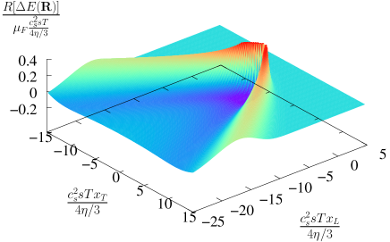
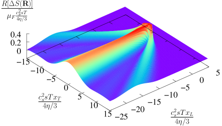
Figure 1: (a) The energy density distribution, $R\,[\Delta E(\mathbf{R})]/[\mu_{F}(c_{s}^{2}sT)/(4\eta/3)]$ and (b) the energy flux distribution, $R\,[\Delta S(\mathbf{R})]/[\mu_{F}(c_{s}^{2}sT)/(4\eta/3)]$ given by the Boltzmann equation. They show a smooth transition from the free streaming to the hydrodynamic regime. We can see a Mach cone and a diffusion wake (in the flux distribution) behind the heavy quark. ($\mathbf{R}=x_{T}\hat{\mathbf{x}}+x_{L}\hat{\mathbf{z}}$)

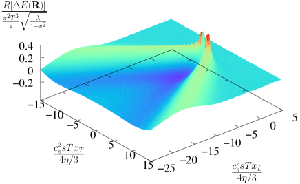
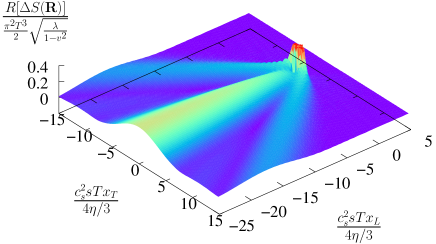
Figure 2: (a) The energy density distribution, $R[\Delta E(\mathbf{R})]/[\pi^{2}T^{3}\sqrt{\lambda/(1-v^{2})}/2]$ and (b) the energy flux distribution, $R[\Delta S(\mathbf{R})]/[\pi^{2}T^{3}\sqrt{\lambda/(1-v^{2})}/2]$ given by the AdS/CFT correspondence. They are singular near the heavy quark at origin. We can see a Mach cone and a diffusion wake (in the flux distribution) behind the heavy quark. ($\mathbf{R}=x_{T}\hat{\mathbf{x}}+x_{L}\hat{\mathbf{z}}$)

In order to analyze the structure, we define the angular distribution with an angle $\theta_{R}$ measured relative to $\hat{\mathbf{z}}$ on $zx$ plane. At a fixed distance $R=|x_{T}\hat{\mathbf{x}}+x_{L}\hat{\mathbf{z}}|$ from the heavy quark, the energy and the momentum density are given by

$$\frac{\rm{d}E_{R}}{\rm{d}\theta_{R}} \equiv 2\pi R^{2}\sin\theta_{R}\,\Delta E(\mathbf{R})\,,$$

$$\frac{\rm{d}S_{R}}{\rm{d}\theta_{R}} \equiv 2\pi R^{2}\sin\theta_{R}\,\hat{\mathbf{R}}\cdot\Delta\mathbf{S}(\mathbf{R})\,,$$ (20)

where $\Delta E\equiv\delta T^{00}$ and $\Delta S_{i}\equiv\delta T^{0i}$. The results are shown in  Figure 3, where distances ($R$) are measured compared to the shear length, $\eta/(sT)$. Generally, the Boltzmann equation and the AdS/CFT correspondence give similar distributions with a Mach cone and a diffusion wake, except for $\mathcal{R}=1$. At short distances, the AdS/CFT solutions are dominated by the zero temperature contribution which is absent in the Boltzmann formulation.

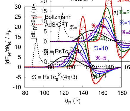
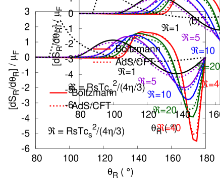
Figure 3: The angular distribution of (a) the energy density $[\rm{d}E_{R}/\rm{d}\theta_{R}]/\mu_{F}$ and (b) the energy flux $[\rm{d}S_{R}/\rm{d}\theta_{R}]/\mu_{F}$ at distances $\mathcal{R}=1,\,5,\,10,\,20,\,\mbox{and}\,40$. The Boltzmann results are compared with the AdS/CFT results. The distance from the heavy quark is measured compared to the shear length, $\eta/(sT)$. At $\mathcal{R}=1$, the AdS/CFT results are dominated by the zero temperature contribution which is absent in the Boltzmann formulation. $\mu_{F}$ for the Boltzmann equation corresponds to $\pi T^{2}\sqrt{\lambda/(1-v^{2})}/2$ for the AdS/CFT correspondence.

IV Hydrodynamics

Hydrodynamics is an effective theory at long distances and is given by the conservation of the energy-momentum tensor

$$T_{hydro}^{\mu\nu}=[e(T)+\mathcal{P}(T)]u^{\mu}u^{\nu}+\mathcal{P}(T)g^{\mu\nu}+\pi^{\mu\nu}\,,$$ (21)

where the first two terms on the right hand side correspond to the ideal hydrodynamics and the last term is the dissipative part. The heavy quark perturbs it away from equilibrium

$$e(t,\mathbf{x})\simeq e_{o}+\delta e(t,\mathbf{x})\,,\qquad u^{\mu}(t,\mathbf{x})\simeq(1,\mathbf{u}(t,\mathbf{x}))\,,$$ (22)

where $\delta e$ and $\mathbf{u}$ are the first order disturbance. In the linearized conformal limit, the dissipative part is given by the first and second order derivative of the fields Baier:2007ix

$$\pi^{\mu\nu}=-2\eta\langle\partial^{\mu}u^{\nu}\rangle-2\eta\tau_{\pi}\langle\partial^{\mu}\partial^{\nu}\ln T\rangle\,\qquad\qquad\mbox{(Static)}\,,$$ (23)

where $\langle\,\cdots\,\rangle$ denotes the symmetric and traceless spatial component. The second order term can be replaced by the leading order relation, making it as a dynamical equation

$$\pi^{\mu\nu}=-2\eta\langle\partial^{\mu}u^{\nu}\rangle-\tau_{\pi}\partial_{t}\pi^{\mu\nu}\,\qquad\qquad\mbox{(Dynamic)}\,.$$ (24)

With the constituent relation, we solve the equation of motion in presence of the external force (minus the drag force)

$$\partial_{\mu}T^{\mu\nu}=F_{micro}^{\nu}\,.$$ (25)

In this case, the force $F_{micro}^{\nu}=\rm{d}p^{\nu}/\rm{d}t$ is given by

$$F_{micro}^{\nu}=\int_{\mathbf{p}}p^{\nu}S(t,\mathbf{x},\mathbf{p})=\mu_{F}v^{\nu}\delta^{3}(\mathbf{x}-\mathbf{v}t)\,,$$ (26)

where $v^{\nu}=(v^{2},\mathbf{v})$.

At long distances from the quark, the stress-energy tensor is described by $T_{hydro}^{\mu\nu}$ and at short distances, we have to consider correction $\tau^{\mu\nu}$ which is localized near the quark

$$T^{\mu\nu}=T_{hydro}^{\mu\nu}+\tau^{\mu\nu}.$$ (27)

Then the equation of motion in Fourier space becomes

$$-i\omega\,\delta T^{0j}+ik^{i}\,\delta T_{hydro}^{ij}=F_{micro}^{j}-ik^{i}\tau^{ij}$$ (28)

and the correction part acts as a source. In the second order, $\tau^{ij}$ can be written with three symmetric tensors consisting of $\mathbf{v}$ and $\mathbf{k}$

$$\tau^{ij} = 2\pi\mu_{F}\,\delta(\omega-\mathbf{v}\cdot\mathbf{k})\,\left[\,\left(v^{i}v^{j}-\frac{1}{3}v^{2}\delta^{ij}\right)\,\phi_{1}(\omega,k^{2})\right.$$ (29)

$$\qquad\qquad\qquad\qquad\quad+\left.\left(iv^{i}k^{j}+ik^{i}v^{j}-\frac{2}{3}i(\mathbf{v}\cdot\mathbf{k})\delta^{ij}\right)\,\phi_{2}(\omega,k^{2})+\left(k^{i}k^{j}-\frac{1}{3}k^{2}\delta^{ij}\right)\,\phi_{3}(\omega,k^{2})\,\right],\qquad$$

where $\phi_{i}(\omega,k^{2})$ $(i=1,2,3)$ is analytic near $\omega=\mathbf{k}=0$. Since $\tau^{ij}$ is localized, we can expand it for small $\omega$ and $\mathbf{k}$

$$-ik^{i}\tau^{ij} = 2\pi\mu_{F}\,\delta(\omega-\mathbf{v}\cdot\mathbf{k})\left[\,-i\phi_{1}(0,0)\,\omega v^{j}+\frac{1}{3}iv^{2}\phi_{1}(0,0)\,k^{j}+\frac{\partial\phi_{1}(0,0)}{i\partial\omega}\omega^{2}v^{j}\right.$$ (30)

$$\qquad\qquad\qquad\qquad\quad+\left.\frac{1}{3}\left(-v^{2}\frac{\partial\phi_{1}(0,0)}{i\partial\omega}+\phi_{2}(0,0)\right)\omega k^{j}+\phi_{2}(0,0)k^{2}v^{j}\,\right]+\mathcal{O}(k^{3})\,.$$

We determine $\tau^{\mu\nu}$ by comparing the numerical solution $T^{\mu\nu}$ with the constituent relation $T_{hydro}^{\mu\nu}$. By comparing order by order, all of the coefficients are numerically determined.  Table 1 shows the result where the coefficients are measured compared to the shear length unit $[R]=[(4\eta/3)/(c_{s}^{2}sT)]$. Note that $\phi_{1}(0,0)$ and $\frac{\partial\phi_{1}(0,0)}{i\partial\omega}$ vanish for the Boltzmann equation. Since the source $S(\mathbf{p})$ in Eq. (15) does not have $H_{l,\pm 2}$ components which correspond to the tensor $\left[v^{i}v^{j}-\frac{1}{3}v^{2}\delta^{ij}\right]$, there is no $\phi_{1}(\omega,k^{2})$ in the Boltzmann case.

Table 1: The correction to the source. $[R]=\left[\frac{4\eta/3}{c_{s}^{2}sT}\right]$

	$\phi_{1}(0,0)$ [$R$]	$\frac{\partial\phi_{1}(0,0)}{i\partial\omega}$ [$R^{2}$]	$\phi_{2}(0,0)$ [$R^{2}$]
Boltzmann	0	0	0.48
AdS/CFT	-1	0.34	-0.33

With the corrected force $F_{micro}^{j}-ik^{i}\tau^{ij}\equiv 2\pi\mu_{F}\delta(\omega-\mathbf{v}\cdot\mathbf{k})[\mathbf{v}\,\phi_{v}(\omega,k^{2})+i\mathbf{k}\,\phi_{k}(\omega,k^{2})]$ Chesler:2007sv , we solve the equation of motion with $v=1$

$$-i\omega\,\delta T^{00}+ik\,\delta T^{0z^{\prime}} = 2\pi\mu_{F}\,\delta(\omega-\mathbf{v}\cdot\mathbf{k})\,,$$

$$-i\omega\,\delta T^{0z^{\prime}}+ic^{2}(k)k\,\delta T^{00}+\Gamma_{s}(\omega)k^{2}\,\delta T^{0z^{\prime}} = \left[\cos\theta\,\phi_{v}+ik\,\phi_{k}\right]2\pi\mu_{F}\,\delta(\omega-\mathbf{v}\cdot\mathbf{k})\,,$$

$$-i\omega\,\delta T^{0x^{\prime}}+D(\omega)k^{2}\,\delta T^{0x^{\prime}} = \sin\theta\,\phi_{v}\,2\pi\mu_{F}\,\delta(\omega-\mathbf{v}\cdot\mathbf{k})\,,$$ (31)

where $\phi_{v}(\omega,k^{2})$ and $\phi_{k}(\omega,k^{2})$ are expanded around $\omega=\mathbf{k}=0$ depending on the order and $c^{2}(k)=c_{s}^{2}=1/3$ is the speed of sound, $\Gamma_{s}(\omega)=\Gamma_{s}=(4\eta/3)/(sT)$ is the sound attenuation length, and $D(\omega)=D=\eta/(sT)$ is the diffusion constant in the first order hydrodynamics. In the second order static hydrodynamics (Eq. (23)), we have same constants except $c^{2}(k)=c_{s}^{2}(1+\tau_{\pi}\Gamma_{s}k^{2})$ while the exception for the dynamic case (Eq. (24)) is $\Gamma_{s}(\omega)=\Gamma_{s}/(1-i\tau_{\pi}\omega)$ and $D(\omega)=D/(1-i\tau_{\pi}\omega)$. The hydrodynamic solutions are given by

$$\delta T^{00}(\omega,\mathbf{k}) = \frac{i\left[\omega+k\cos\theta\,\phi_{v}\right]-k^{2}\left[\Gamma_{s}(\omega)+\phi_{k}\right]}{\omega^{2}-c^{2}(k)\,k^{2}+i\Gamma_{s}(\omega)\,\omega k^{2}}\,2\pi\mu_{F}\delta(\omega-k\cos\theta)\,,$$

$$\delta T^{0z^{\prime}}(\omega,\mathbf{k}) = \frac{i\left[\,\omega\cos\theta\,\phi_{v}+c^{2}(k)\,k\,\right]-k\omega\,\phi_{k}}{\omega^{2}-c^{2}(k)\,k^{2}+i\Gamma_{s}(\omega)\,\omega k^{2}}\,2\pi\mu_{F}\delta(\omega-k\cos\theta)\,,$$

$$\delta T^{0x^{\prime}}(\omega,\mathbf{k}) = \frac{i\sin\theta\,\phi_{v}}{\omega+iD(\omega)\,k^{2}}\,2\pi\mu_{F}\delta(\omega-k\cos\theta)\,.$$ (32)

In  Figure 4, 5, we compare hydrodynamic results to the full theory. The difference between the static and the dynamic solution is shown in  Figure 6.

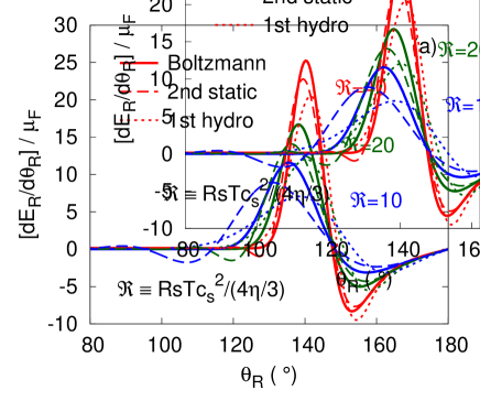
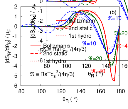
Figure 4: The angular distribution of (a) the energy density $[\rm{d}E_{R}/\rm{d}\theta_{R}]/\mu_{F}$ and (b) the energy flux $[\rm{d}S_{R}/\rm{d}\theta_{R}]/\mu_{F}$ given by the Boltzmann equation at distances $\mathcal{R}=10,\,20,\,\mbox{and}\,40$. The Boltzmann results are compared with the first order and the second order static hydrodynamics.

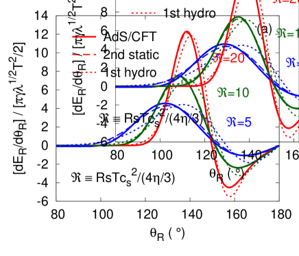
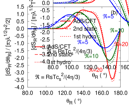
Figure 5: The angular distribution of (a) the energy density $[\rm{d}E_{R}/\rm{d}\theta_{R}]/[\pi\gamma\sqrt{\lambda}T^{2}/2]$ and (b) the energy flux $[\rm{d}S_{R}/\rm{d}\theta_{R}]/[\pi\gamma\sqrt{\lambda}T^{2}/2]$ given by the AdS/CFT correspondence at distances $\mathcal{R}=5,\,10,\,\mbox{and}\,20$. The AdS/CFT results are compared with the first order and the second order static hydrodynamics. ($\gamma=1/\sqrt{1-v^{2}}$)

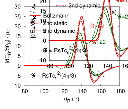
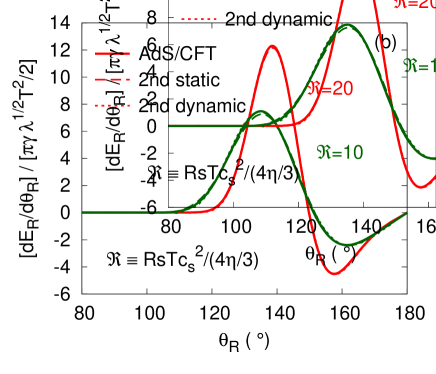
Figure 6: (a) The angular distribution of the energy density, $[\rm{d}E_{R}/\rm{d}\theta_{R}]/\mu_{F}$ given by the Boltzmann equation at distances $\mathcal{R}=20,\,40$. The Boltzmann results are compared with the second order static and dynamic hydrodynamics. The dynamic solution develops spurious shocks for $\mathcal{R}<20$. (b) The angular distribution of the energy density, $[\rm{d}E_{R}/\rm{d}\theta_{R}]/[\pi\gamma\sqrt{\lambda}T^{2}/2]$ given by the AdS/CFT correspondence at distances $\mathcal{R}=10,\,20$. The AdS/CFT results are compared with the second order static and dynamic hydrodynamics. ($\gamma=1/\sqrt{1-v^{2}}$)

V Discussion

We presented the energy density and flux distribution given by kinetic theory based on the Boltzmann equation at weak coupling, and compared them with those given by the AdS/CFT correspondence at strong coupling. Both of them show a Mach cone and diffusion wake at long distances but their behaviors are distinguishable by the approach to the hydrodynamic limit.

In the Boltzmann equation, the second order static hydrodynamics (Eq. (23)) works better than first order for $\mathcal{R}\gtrsim 40$, but it is unnatural for $\mathcal{R}\lesssim 10$ due to the high frequency behavior. In principle, the second order dynamic solution (Eq. (24)) is better than static one at long distances (see  Figure 6 (a)). However, the dynamic solution has higher order terms and develops spurious shocks for $\mathcal{R}<20$.

In the AdS/CFT correspondence, even the first order hydrodynamics is good for $\mathcal{R}\gtrsim 5$. Only the sound wave has corrections of the second order static hydrodynamics and is dominant in the energy distribution. At $\mathcal{R}=5$ in the energy density, we can see the improvement given by the second order theory. Both the static and the dynamic solution work very well in  Figure 6 (b).

In comparison with the AdS/CFT correspondence, the Boltzmann equation produces a smooth transition from the free streaming to the hydrodynamic regime. The stress-energy tensor given by the AdS/CFT correspondence is significantly better described by hydrodynamics in the sub-asymptotic regime. Although they have different sources, we believe that this difference is due to the second order hydrodynamic coefficient, $\tau_{\pi}$. Compared to the shear length, they are given by

$$\tau_{\pi}\simeq 1.58\left[\frac{4\eta/3}{c_{s}^{2}sT}\right]\quad\mbox{(Boltzmann)}\,\quad\qquad\longleftrightarrow\qquad\quad\tau_{\pi}\simeq 0.65\left[\frac{4\eta/3}{c_{s}^{2}sT}\right]\quad\mbox{(AdS/CFT)}\,.$$ (33)

The coefficient $\tau_{\pi}$ in unit of $\eta/(sT)$ is generically $\sim 2.4$ times larger in the Boltzmann equation than in gauge/gravity duality. As a result, the hydrodynamic solutions are more reactive to the high frequencies and it takes longer to reach the hydrodynamic regime, in a relative sense, in the Boltzmann equation.

- (1) S. S. Gubser and S. S. Pufu and A. Yarom, Phys. Rev. Lett. 100, 012301 (2008) [arXiv:0706.4307 [hep-th]].
- (2) P. M. Chesler and L. Yaffe, Phys. Rev. D 78, 045013 (2008) [arXiv:0712.0050 [hep-th]].
- (3) P. Arnold, G. D. Moore and L. G. Yaffe, JHEP 0011, 001 (2000) [arXiv:hep-ph/0010177].
- (4) J. Hong and D. Teaney, Phys. Rev. C 82, 044908 (2010) [arXiv:1003.0699 [nucl-th]].
- (5) P. Arnold, C. Dogan and G. D. Moore, Phys. Rev. D 74, 085021 (2006) [arXiv:hep-ph/0608012].
- (6) P. Kovtun, D. T. Son and A. O. Starinets, Phys. Rev. Lett. 94, 111601 (2005) [arXiv:hep-th/0405231].
- (7) R. Baier, P. Romatschke, D. T. Son, A. O. Starinets, and M. A. Stephanov, JHEP 04, 100 (2008) [arXiv:0712.2451 [hep-th]].