Geodesic Structure of the Noncommutative Schwarzschild Anti-de Sitter Black Hole I: Timelike Geodesics

Abstract

By considering particles as smeared objects, we investigate the effects of space noncommutativity on the geodesic structure in Schwarzschild-AdS spacetime. By means of a detailed analysis of the corresponding effective potentials for particles, we find the possible motions which are allowed by the energy levels. Radial and non-radial trajectories are treated and the effects of space noncommutativity on the value of the precession of the perihelion are estimated. We show that the geodesic structure of this black hole presents new types of motion not allowed by the Schwarzschild spacetime.

PACS: 02.40.Gh, 04.70.Bw, 04.20.q, 02.40.-k

Keywords: Noncommutative geometry, classical black holes, general gelativity

I Introduction

The presence of a vacuum energy (cosmological constant) in theoretical models has been considered in relation to unification, such as superstring theory, and to cosmology and astrophysics. This has motivated consideration of spherical symmetric spacetimes with non-zero vacuum energy in order to study the well-known effects predicted by general relativity for planetary orbits and massless particles. This study implies the determination of the geodesic structure of spacetimes kottler . Timelike geodesics for a positive cosmological constant were investigated in key-2 using an effective potential method to find the conditions for the existence of bound orbits. The analysis of the effective potential for radial null geodesic in Reissner–Nordstrom–deSitter and Kerr–deSitter spacetime was realized in key-4 and key-5 . Podolsky key-6 investigated all possible geodesic motions for extreme Schwarzschild–de Sitter spacetime. Finally, Cruz et.al. key-7 made a complete disussion on the geodesic structure of Schwarzschild-anti de Sitter (Schw-AdS) black hole.

On the other hand, gedanken experiments that aim at probing spacetime structure at very small distances support the idea that noncommutativity of spacetime is a feature of Planck scale physics. It appears to happen that due to gravitational back reaction, one cannot test spacetime at Planck scale. Its description as a smooth manifold becomes therefore a mathematical assumption no more justified by physics and therefore, it is natural to relax this assumption and conceive a more general noncommutative spacetime, where uncertainty relations and discretization naturally arise.

As is well known, noncommutativity is the central mathematical concept expressing uncertainty in quantum mechanics, where it applies to any pair of conjugate variables, such as position and momentum. Thus, one can easily imagine that position measurements might fail to commute and this fact will be described using noncommutativity of spacetime coordinates. The noncommutativity of spacetime coordinates can be encoded in the commutator NC1 ; NC2 ; NC3 ; NC4 ; NC5 ; NC6 ; NC7 ; NC8

$$\left[x^{\mu},x^{\nu}\right]=i\varepsilon^{\mu\nu}$$ (1)

where $\varepsilon^{\mu\nu}$ is a real, antisymmetric and constant tensor, which determines the fundamental cell discretization of spacetime (in the same way as the Planck constant $\hbar$ discretizes the phase space). In four dimensions and using an adequate choice of coordinates, this tensor can be brought to the form

$$\varepsilon^{\mu\nu}=\left(\begin{array}[]{cccc}0&\varepsilon^{2}&0&0\\ -\varepsilon^{2}&0&\varepsilon^{2}&0\\ 0&-\varepsilon^{2}&0&\varepsilon^{2}\\ 0&0&-\varepsilon^{2}&0\end{array}\right),$$ (2)

where $\varepsilon$ is a constant with dimension of length.

The modifications induced by noncommutativity on the classical orbits of particles in a central force potential has been considered by Benczik et al NCg1 , by Mirza and Dehghani NCg2 and by Romero and Vergara NCg3 . These investigations let them impose a constraint on the minimal observable length and noncommutativity parameter in comparison with observational data of Mercury. The stability of planetary orbits of particles in noncommutative space has been studied both in central force and Schwarzschild background by Nozari and Akhshabi NCg4 and the Kepler problem in noncommutative Schwarzschild geometry in NCg5 . The purpose of this paper is to investigate these effects on the orbits of a test particle in noncommutative Schwarzschild-AdS (NCSchw-AdS) geometry to generalize the geodesic structure studied in key-7 .

II The Noncommutative Schwarzschild-AdS Black HOle

It has been shown that noncommutativity eliminates point-like structures in favor of smeared objects in flat spacetime NCBH0 ; NCBH1 . The effect of smearing can be mathematically implemented as a substitution rule: position Dirac-delta function can be replaced everywhere with a Gaussian distribution of minimal width $\varepsilon$. In this framework, the mass density of a static, spherically symmetric, smeared, particle-like gravitational source can be shown by a Gaussian profile NCBH ; NCBH2 ; NCBH3 ; NCBH4 . Solving the Einstein field equations, one can find the metric for a static spherically symmetric object with total mass $M$ in a noncommutative spacetime with negative cosmological constant $\text{\leavevmode{L}}=-\frac{3}{L^{2}}$ as NCSadS

$$ds^{2}=-f\left(r\right)dt^{2}+\frac{dr^{2}}{f\left(r\right)}+r^{2}d\Omega^{2}$$ (3)

where the lapse function is

$$f\left(r\right)=1-\frac{4M\gamma\left(\frac{3}{2};\frac{r^{2}}{4\varepsilon^{2}}\right)}{r\sqrt{\pi}}+\frac{r^{2}}{L^{2}}$$ (4)

and $\gamma$ is the lower incomplete gamma function,

$$\gamma\left(\frac{3}{2};x\right)=\int_{0}^{x}dtt^{1/2}e^{-t}.$$ (5)

The horizon equation $f\left(r_{+}\right)=0$ depends on two parameters, $M$ and $L$ and cannot be solved in a closed form. However, we can draw plots to study the occurrence of horizons. In order to do it, we will write the lapse function as

$$f\left(x\right)=1-\frac{4m\gamma\left(\frac{3}{2};\frac{x^{2}}{q^{2}}\right)}{x\sqrt{\pi}}+x^{2}$$ (6)

where we have defined $x=\frac{r}{L}$, $m=\frac{MG}{L}$ and $q=\frac{2\varepsilon}{L}$. In Figure 1 the plot of $f\left(x\right)$ show that all curves start at $f\left(0\right)=1$, indicating that the spacetime is regular and therefore geodesically complete. The behavior of the curves shows three possibilities,

1. For $m>m_{0}$ there are two horizons, $x_{-}$ and $x_{+}$ (i.e. $r_{-}$ and $r_{+}$ )

2. For $m=m_{0}$ there is one degenerate horizon, $x_{0}$ (i.e. $r_{0}$ )

3. For $m<m_{0}$ there is no horizon.

The critical value $m_{0}$ depends on $\varepsilon$ and $L$ and is determined by the conditions

$$f\left(x\right)=\frac{\partial f}{\partial x}=0.$$ (7)

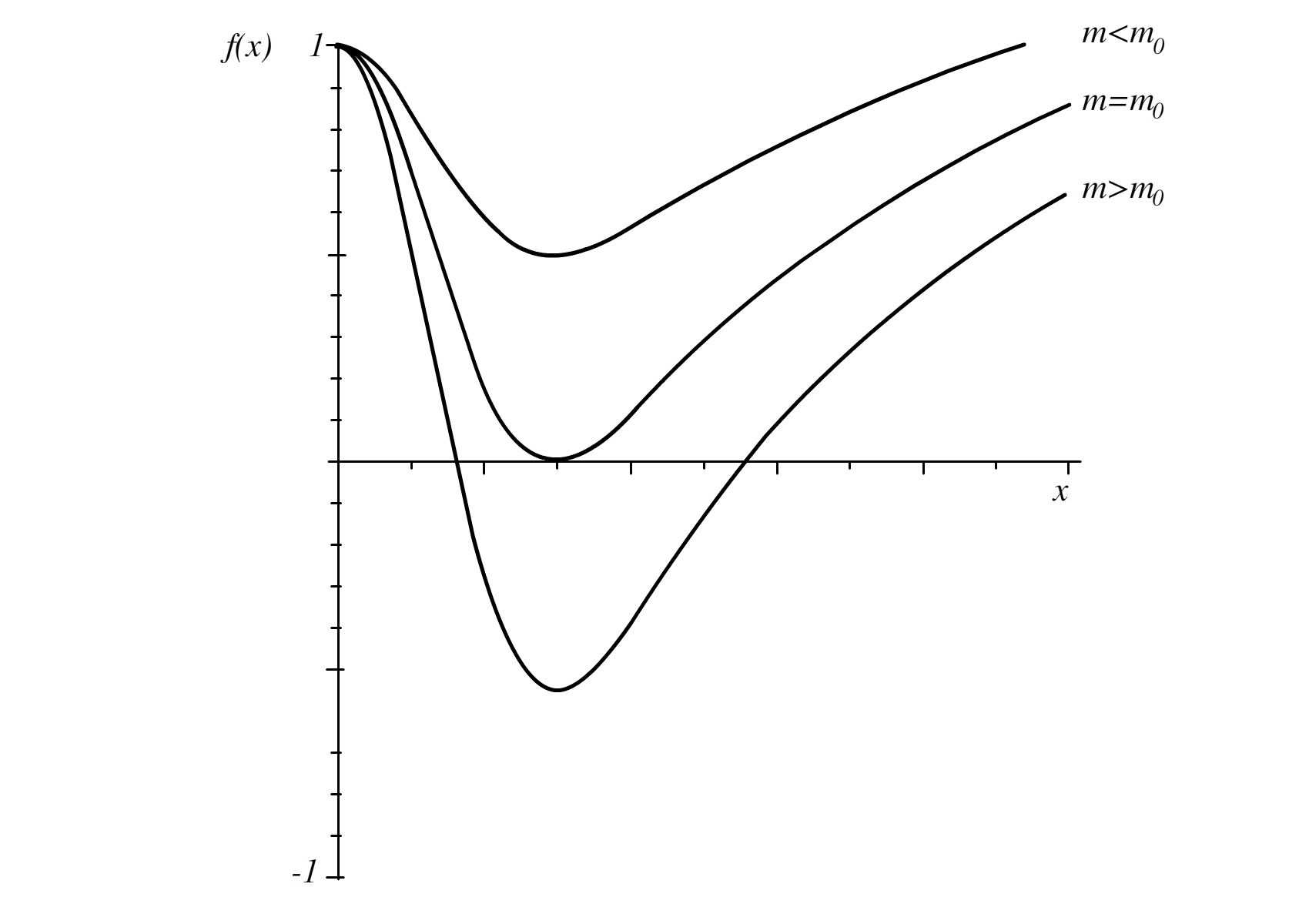
Figure 1: $f\left(x\right)$ for different values of $m$. We notice that there exist three cases, namely two horizons, no horizon and one single degenerate horizon.

III TimeLike Geodesics

In order to find the geodesics structure of the spacetime described by (3), we solve the Euler-Lagrange equations for the variational problem associated to this metric adler . The Lagrangian is

$$\mathcal{L}=-f\left(r\right)\dot{t}^{2}+\frac{\dot{r}^{2}}{f\left(r\right)}+r^{2}\dot{\theta}^{2}+r^{2}\sin^{2}\theta\dot{\varphi}^{2}$$ (8)

where the dots represent the derivative with respect to the affine parameter $\tau$, along the geodesic. The equations of motion are

$$\dot{\pi}_{q}=\frac{d}{dt}\left(\frac{\partial\mathcal{L}}{\partial\dot{q}}\right)=\frac{\partial\mathcal{L}}{\partial q}.$$ (9)

Since $\mathcal{L}$ is independient of $t$ and $\varphi$ there are two conserved quantities,

$$E=-\frac{\pi_{t}}{2}=f\left(r\right)\dot{t}$$ (10)

and

$$\ell=\frac{\pi_{\varphi}}{2}=r^{2}\sin^{2}\theta\dot{\varphi}.$$ (11)

Meanwhile, the equation of motion for $\theta$ gives

$$\frac{d(r^{2}\dot{\theta})}{d\tau}=r^{2}sin\theta cos\theta\dot{\phi}^{2}.$$ (12)

Therefore, if we choose the initial condition $\theta=\frac{\pi}{2}$ and $\dot{\theta}=0$, the last equation gives $\ddot{\theta}=0$. This means that the motion is confined to the plane $\theta=\frac{\pi}{2}$ , which is characteristic of central fields. With this election, the angular momentum is

$$\ell=r^{2}\dot{\varphi}$$ (13)

and the Lagrangian becomes

$$\mathcal{L}=-h=-\frac{E^{2}}{f\left(r\right)}+\frac{\dot{r}^{2}}{f\left(r\right)}+\frac{\ell^{2}}{r^{2}},$$ (14)

where we shall consider $h=1$ for massive particles and $h=0$ for photons. Solving the above equation for $\dot{r}^{2}$ we obtain the radial equation which allow us to characterize possible movements of test particles without and explicit solution of the equation of motion in the invariant plane. This is

$$\dot{r}^{2}=E^{2}-f\left(r\right)\left(h+\frac{\ell^{2}}{r^{2}}\right)$$ (15)

or better

$$\dot{r}^{2}=E^{2}-V_{eff}^{2}$$ (16)

with the effective potential

$$V_{eff}^{2}\left(r\right)=\left(1-\frac{4M\gamma\left(\frac{3}{2};\frac{r^{2}}{4\varepsilon^{2}}\right)}{r\sqrt{\pi}}+\frac{r^{2}}{L^{2}}\right)\left(h+\frac{\ell^{2}}{r^{2}}\right).$$ (17)

For timelike geodesics, $h=1$, the effective potential becomes

$$V_{eff}^{2}\left(r\right)=\left(1-\frac{4M\gamma\left(\frac{3}{2};\frac{r^{2}}{4\varepsilon^{2}}\right)}{r\sqrt{\pi}}+\frac{r^{2}}{L^{2}}\right)\left(1+\frac{\ell^{2}}{r^{2}}\right).$$ (18)

$V_{eff}^{2}\left(r\right)$ let us solve the equation of motion for two interesting special cases of massive particle orbits, namely radial motion and bound orbits.

III.1 Radial Geodesics

For radial geodesics, $\ell=0$, we have

$$V_{eff}^{2}\left(r\right)=1-\frac{4M\gamma\left(\frac{3}{2};\frac{r^{2}}{4\varepsilon^{2}}\right)}{r\sqrt{\pi}}+\frac{r^{2}}{L^{2}}.$$ (19)

The behavior of the effective potential is shown in Figure 2. Note that in Figure 2 (a) (with $L=1$ and $M=1$) the particle always moves towards $r=0$; but for greater $M$ or greater $L$ (i.e. smaller $\Lambda$), the function $V_{eff}^{2}$ has a minimum. Therefore, for certain values of the energy of the particle moving radially, it can not reach $r=0$ but is repelled once it has approached to within some finite distance.

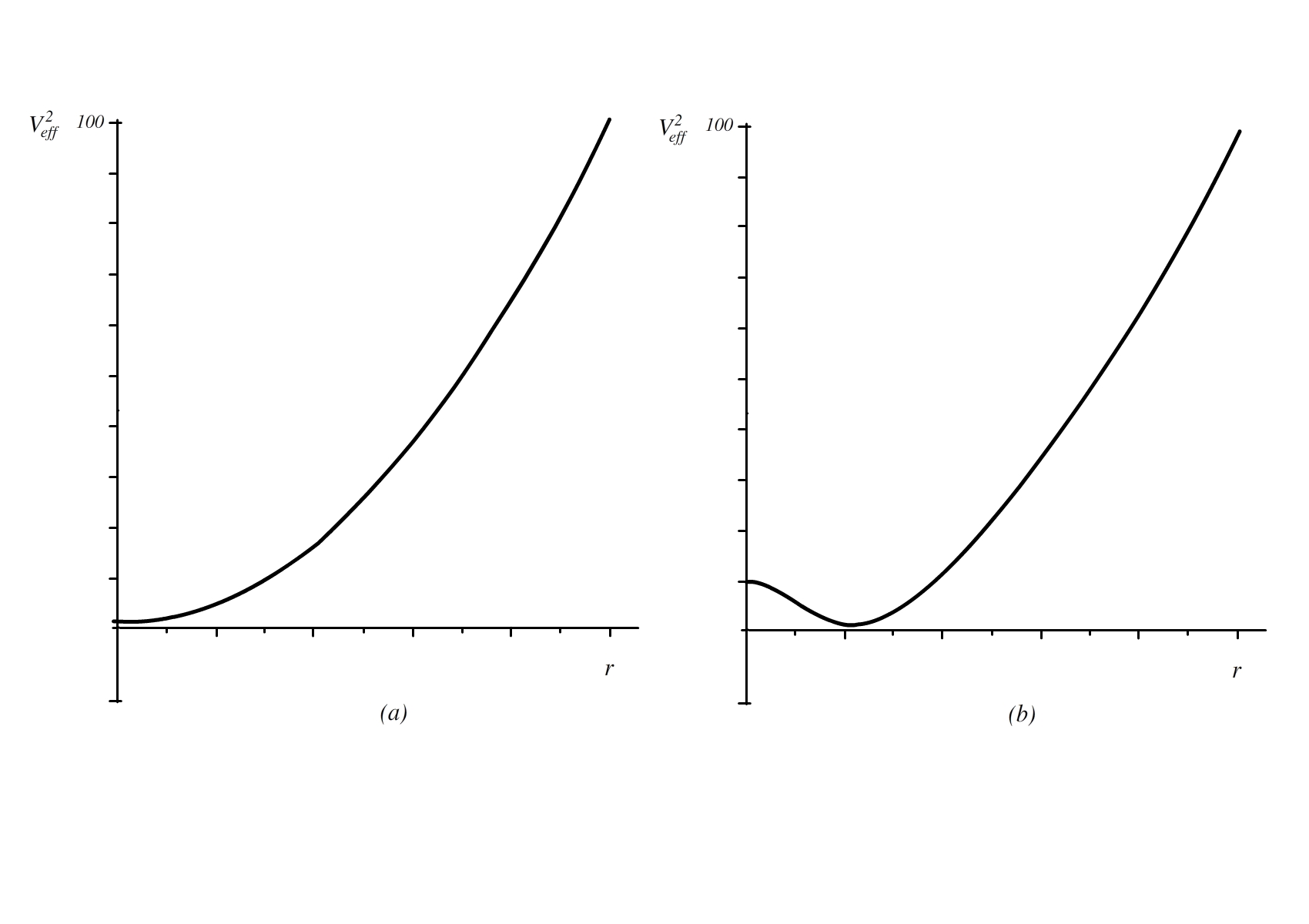
Figure 2: The effective potential for radial particles. For figure (a) we use $\varepsilon=1$ and $L=1$ while figure (b) has $\varepsilon=1$ and $L=10$ in arbitrary units.

In the curve representing $V_{eff}^{2}$, particles always plunge into the horizon from an upper distance determined by the constant of motion $E$. If the particle is release from rest at a distance $r=r_{i}$ we have the constant

$$E^{2}=V_{eff}^{2}\left(r_{i}\right)=1-\frac{4M\gamma\left(\frac{3}{2};\frac{r_{i}^{2}}{4\varepsilon^{2}}\right)}{r_{i}\sqrt{\pi}}+\frac{r_{i}^{2}}{L^{2}}$$ (20)

and the equation of motion can be written as

$$\dot{r}^{2}=\frac{4M}{\sqrt{\pi}}\left[\frac{\gamma\left(\frac{3}{2};\frac{r^{2}}{4l^{2}}\right)}{r}-\frac{\gamma\left(\frac{3}{2};\frac{r_{i}^{2}}{4\varepsilon^{2}}\right)}{r_{i}}\right]-\frac{1}{L^{2}}\left(r^{2}-r_{i}^{2}\right)$$ (21)

which can be integrated as

$$\tau\left(r\right)=\int_{r_{i}}^{r}\frac{dr}{\sqrt{\frac{4M}{\sqrt{\pi}}\left[\frac{\gamma\left(\frac{3}{2};\frac{r^{2}}{4\varepsilon^{2}}\right)}{r}-\frac{\gamma\left(\frac{3}{2};\frac{r_{i}^{2}}{4\varepsilon^{2}}\right)}{r_{i}}\right]-\frac{1}{L^{2}}\left(r^{2}-r_{i}^{2}\right)}}$$ (22)

to give the proper time experienced by a particle in falling from $r_{i}$ to a coordinate radius $r$. Equation (22) is plotted in Figure 3 and show that the particle falls towards the horizon in a finite proper time smaller than that corresponding to the Schwarzschild-AdS case.

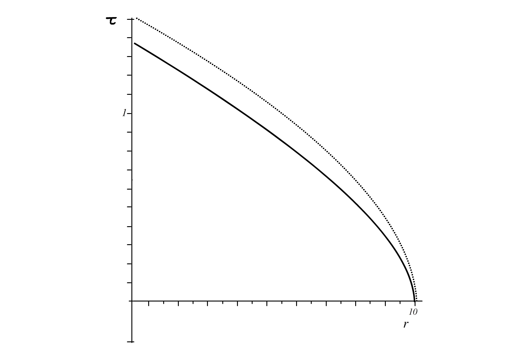
Figure 3: Proper time $\tau$ as a function of $r$. The dotted curve corresponds to the Schwarzschild-AdS metric while the continuous curve is the noncummutative black hole. In this case $r_{i}=10$.

III.2 The Bound Orbits

In this case $\ell\neq 0$, and

$$V_{eff}^{2}\left(r\right)=\left(1-\frac{4M\gamma\left(\frac{3}{2};\frac{r^{2}}{4\varepsilon^{2}}\right)}{r\sqrt{\pi}}+\frac{r^{2}}{L^{2}}\right)\left(1+\frac{\ell^{2}}{r^{2}}\right).$$ (23)

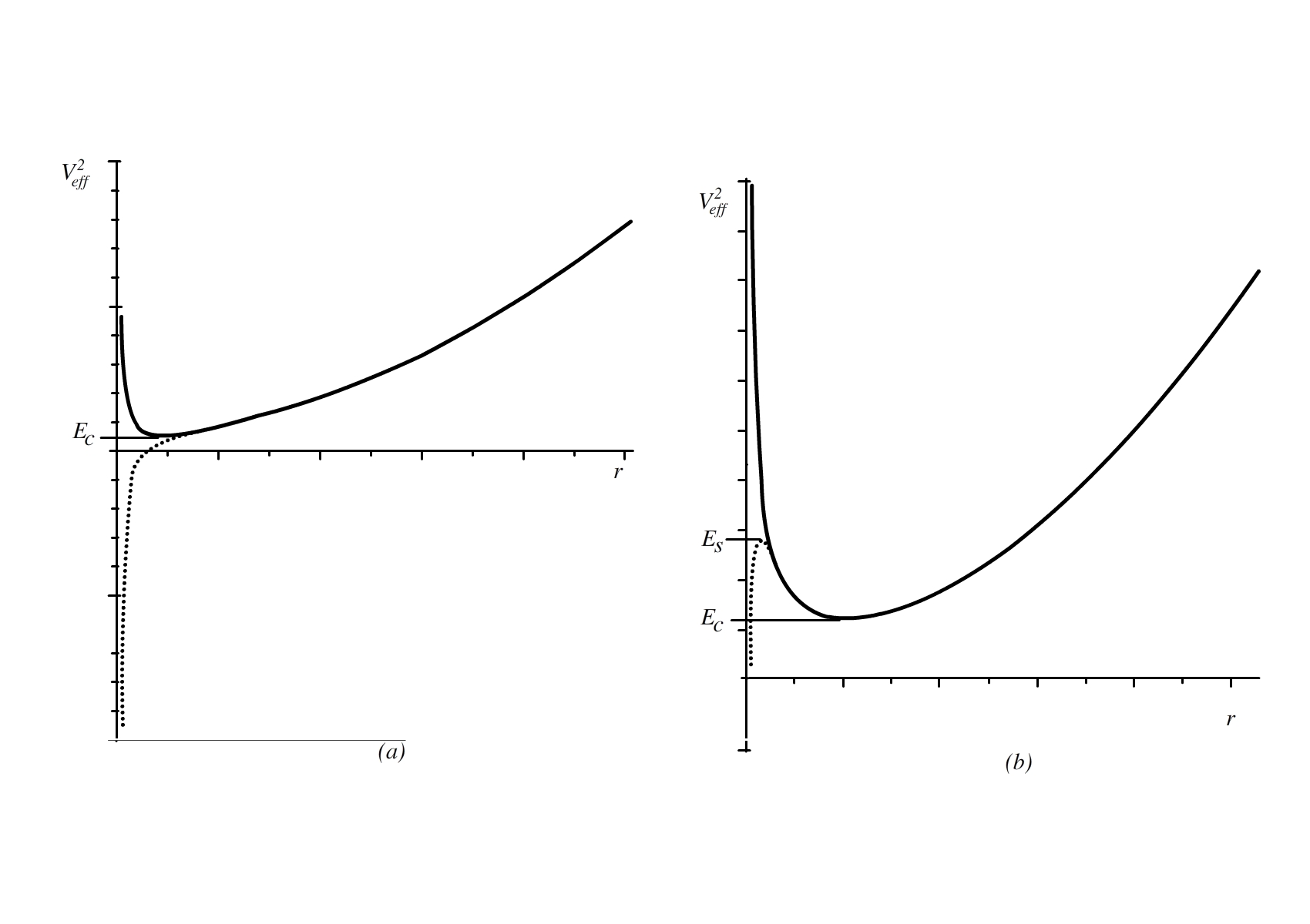
Figure 4: The effective potential for non-radial particles in the Schwarzschild-AdS metric (dotted curve) and non-commutative Schwarzschild-AdS (continuous curve). In figure (a) we set $L=10$, $l=1$ and $\ell=1$ while in figure (b) has $L=10$, $l=1$ and $\ell=15$ in arbitrary units.

In Figure 4, the effective potential has been plotted for non-radial particles and compared to the Schwarzschild-AdS case. Note that for the noncommutative black hole there are always two kinds of allowed orbits, depending on the value of the constant $E$,

1. If $E^{2}=E_{c}^{2}$, the particle orbits in a stable circular orbit at $r=r_{c}$

2. If $E^{2}>E_{c}^{2}$, the particle orbits on a bound orbit in the range $r_{P}<r<r_{A}$ ($r_{P}$ and $r_{A}$ are the perihelion and aphelion distances, respectively),

where $E_{c}^{2}$ corresponds to the minimum value of the effective potential, $E_{c}^{2}=\left.V_{eff}^{2}\right|_{min}$.

In Figure 4 there is a third possibility in Scharzschild-AdS case (dotted curve). When $E^{2}=E_{S}^{2}$, the particle can orbit in an unstable circular orbit. However, this orbit is never allowed for the noncommutative black hole. The divergency of the continuous curve in Figure 4 around the origin is a manifestation of the existence of a minimal lenght scale, which prevents to probe distances smaller that the fundamental distance $\varepsilon$.

The equation of motion is obtained using equations (13) and (16) and making the change of variable $u=\frac{1}{r}$, giving

$$\left(\frac{du}{d\theta}\right)^{2}+u^{2}=\frac{\epsilon^{2}}{\ell^{2}}+\frac{4Mu}{\sqrt{\pi}\ell^{2}}\gamma\left(\frac{3}{2};\frac{1}{4\varepsilon^{2}u^{2}}\right)+\frac{4M}{\sqrt{\pi}}u^{3}\gamma\left(\frac{3}{2};\frac{1}{4\varepsilon^{2}u^{2}}\right)-\frac{1}{L^{2}\ell^{2}u^{2}}$$ (24)

with

$$\epsilon^{2}=E^{2}-1-\frac{\ell^{2}}{L^{2}}.$$ (25)

This expression can be rewritten as

$$\left(\frac{du}{d\theta}\right)^{2}=f\left(u\right)$$ (26)

with

$$f\left(u\right)=\frac{\epsilon^{2}}{\ell^{2}}+\frac{4Mu}{\sqrt{\pi}\ell^{2}}\gamma\left(\frac{3}{2};\frac{1}{4\varepsilon^{2}u^{2}}\right)+\frac{4M}{\sqrt{\pi}}u^{3}\gamma\left(\frac{3}{2};\frac{1}{4\varepsilon^{2}u^{2}}\right)-u^{2}-\frac{1}{L^{2}\ell^{2}u^{2}}.$$ (27)

Considering only orbits which possess perihelia, the point of closest approach is given by the condition

$$\frac{du}{d\theta}=f\left(u\right)=0$$ (28)

and for the rest of the orbit $u$ is less than its perihelion value. Equation (26) tell us that throughout the orbit $f\left(u\right)\geq 0$. In Figure 5 we show three typical situations in which function $f\left(u\right)$ has one and three zeros. Figure 5b corresponds to an elliptical orbit with $u$ oscillating in the range $u_{A}<u<u_{P}$ ($u_{P}$ corresponds to the perihelion while $u_{A}$ is the aphelion). On the other hand, Figure 5c shows the special case in which $u_{A}=u_{P}=u_{c}$ and the orbit becomes a circle.

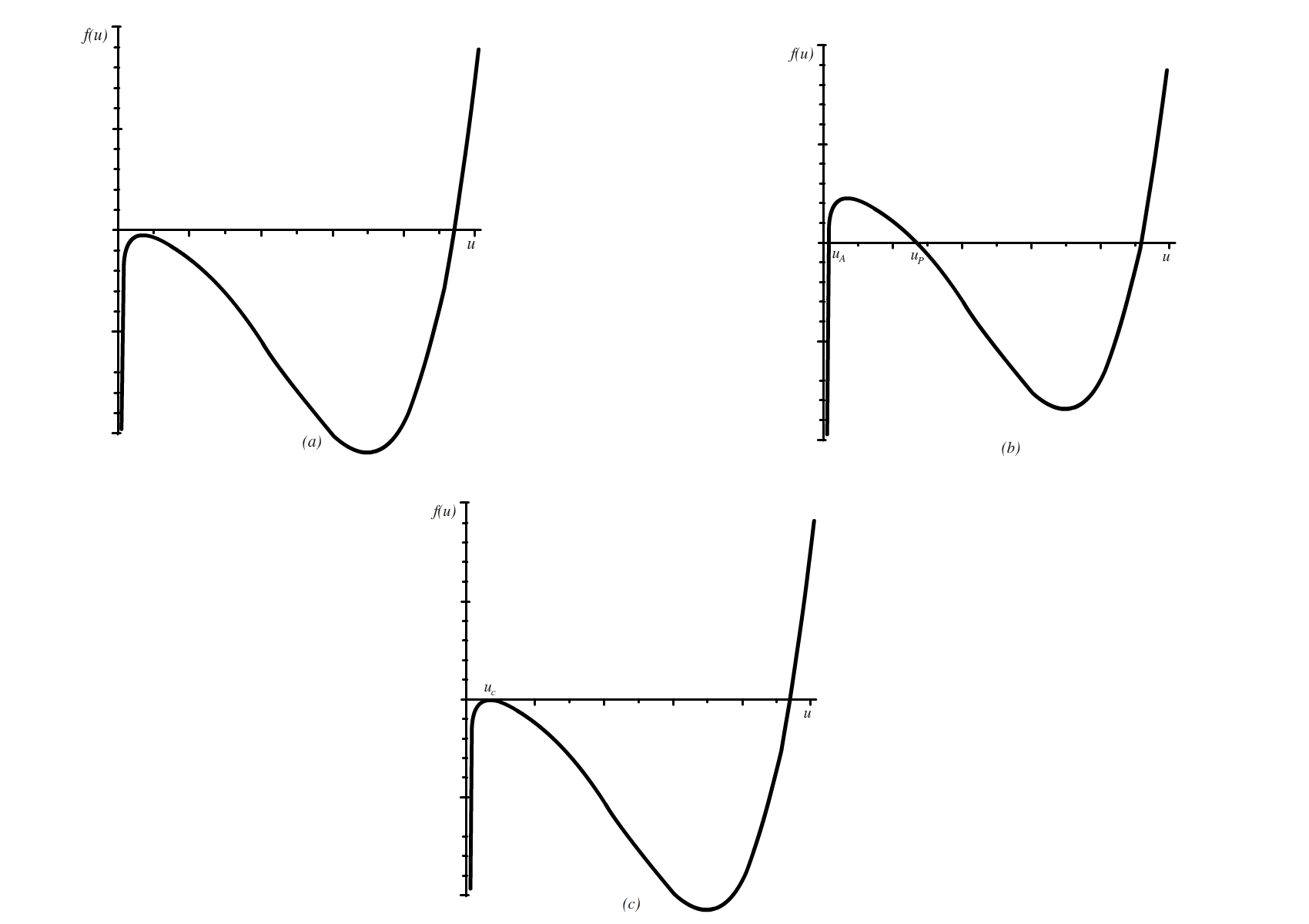
Figure 5: Graphs of the function $f\left(u\right)$. In figure (a) we set $L=10$, $\varepsilon=1$, $\ell=10$ and $\epsilon=0$. Figure (b) has $L=10$, $\varepsilon=1$, $\ell=10$ and $\epsilon=5$ while Figure (c) use $L=10$, $\varepsilon=1$, $\ell=10$ and $\epsilon=1.41$

We now differentiate this equation with respect to $\theta$, using the relation

$$\frac{\partial}{\partial u}\gamma\left(\frac{3}{2},\frac{1}{4\varepsilon^{2}u^{2}}\right)=\frac{e^{-1/4\varepsilon^{2}u^{2}}}{4\varepsilon^{3}u^{4}},$$ (29)

to obtain

$$\frac{d^{2}u}{d\theta^{2}}+u=\frac{2M}{\sqrt{\pi}\ell^{2}}\gamma\left(\frac{3}{2};\frac{1}{4\varepsilon^{2}u^{2}}\right)+\frac{6M}{\sqrt{\pi}}u^{2}\gamma\left(\frac{3}{2};\frac{1}{4\varepsilon^{2}u^{2}}\right)+\frac{1}{L^{2}\ell^{2}u^{3}}+\frac{M}{2\sqrt{\pi}\ell^{5}}\frac{e^{-1/4\varepsilon^{2}u^{2}}}{u^{3}}+\frac{M}{2\sqrt{\pi}\varepsilon^{3}}\frac{e^{-1/4\varepsilon^{2}u^{2}}}{u}.$$ (30)

Approximating the incomplete gamma function for long distances to first order,

$$\gamma\left(\frac{3}{2},\frac{1}{4\varepsilon^{2}u^{2}}\right)\simeq\frac{\sqrt{\pi}}{2}-\frac{1}{2\varepsilon}\frac{e^{-1/4\varepsilon^{2}u^{2}}}{u},$$ (31)

the differential equation of the orbit gives

$$\frac{d^{2}u}{d\theta^{2}}+u=\frac{M}{\ell^{2}}+3Mu^{2}+\frac{1}{L^{2}\ell^{2}u^{3}}+\frac{M}{\sqrt{\pi}}e^{-1/4\varepsilon^{2}u^{2}}\left[\frac{3u}{\varepsilon}+\frac{1}{2u^{3}\ell^{5}}+\frac{1}{\varepsilon u}\left(\frac{1}{2\varepsilon^{2}}+\frac{1}{\ell^{2}}\right)\right].$$ (32)

Note that the third term on the right gives the corrections to the orbit due to the cosmological constant key-7 while the last term gives the corrections due to non-commutative effects. For long distances $\left(u\rightarrow 0\right)$ or small noncommutative scale $\left(\varepsilon\rightarrow 0\right)$, the last term correctly tends to zero giving the orbit analyzed in NCg5 .

III.2.1 Advance of the Perihelion

In order to obtain the advance of the perihelion of a planetary orbit we use the method given in Corn to compare a keplerian ellipse in Lorentzian coordinates with one in noncommutative Schwarzschild-AdS coordinates. The relevant relation communicating the two ellipse is the constant of Kepler’s second law. In Lorentz coordinates the line element is given by

$$ds^{2}=-dt^{2}+dr^{2}+r^{2}(d\theta^{2}+\sin^{2}\theta d\phi^{2}).$$ (33)

The noncommutative Schwarzschild-AdS gravitational field, given by equation (3), allow us to find the following transformation of the coordinates, $r$ and $t$, in the binomial approximation

$$dt^{\prime} = \left(1-\frac{2M\gamma\left(\frac{3}{2};\frac{r^{2}}{4\varepsilon^{2}}\right)}{r\sqrt{\pi}}+\frac{r^{2}}{2L^{2}}\right)dt$$ (34)

$$dr^{\prime} = \left(1+\frac{2M\gamma\left(\frac{3}{2};\frac{r^{2}}{4\varepsilon^{2}}\right)}{r\sqrt{\pi}}-\frac{r^{2}}{2L^{2}}\right)dr,$$ (35)

or using (31),

$$dt^{\prime} = \left(1-\frac{M}{r}-\frac{M}{\sqrt{\pi}\varepsilon}e^{-\frac{r^{2}}{4\varepsilon^{2}}}+\frac{r^{2}}{2L^{2}}\right)dt$$ (36)

$$dr^{\prime} = \left(1+\frac{M}{r}+\frac{M}{\sqrt{\pi}\varepsilon}e^{-\frac{r^{2}}{4\varepsilon^{2}}}-\frac{r^{2}}{2L^{2}}\right)dr.$$ (37)

We consider two elliptical orbits, one the classical Kepler orbit in $\left(r,t\right)$ space and a noncommutative Schwarzschild-AdS orbit in $\left(r^{\prime},t^{\prime}\right)$ space. In the Lorentz space we have

$$dA=\int_{0}^{\rho}rdrd\phi,$$ (38)

and hence the Kepler second law

$$\frac{dA}{dt}=\frac{1}{2}\rho^{2}\frac{d\phi}{dt}.$$ (39)

In the noncommutative Schwarzschild-AdS situation, we have

$$dA^{\prime}=\int_{0}^{\rho}rdr^{\prime}d\phi.$$ (40)

Therefore, using equation (37) the integrand becomes

$$dA^{\prime}=\int_{0}^{\rho}r\left(1+\frac{M}{r}-\frac{M}{\sqrt{\pi}\varepsilon}e^{-\frac{r^{2}}{4\varepsilon^{2}}}-\frac{r^{2}}{2L^{2}}\right)drd\phi$$ (41)

which can be integrated to obtain

$$dA^{\prime}=\frac{\rho^{2}}{2}\left(1+\frac{2M}{\rho}-\frac{\rho^{2}}{4L^{2}}+\frac{4M\varepsilon}{\sqrt{\pi}\rho^{2}}e^{-\frac{\rho^{2}}{4l^{2}}}-\frac{4M\varepsilon}{\sqrt{\pi}\rho^{2}}\right)d\phi.$$ (42)

Hence, using (36), the area law is

$$\frac{dA^{\prime}}{dt^{\prime}}=\frac{\rho^{2}}{2}\left(1+\frac{2M}{\rho}-\frac{\rho^{2}}{4L^{2}}+\frac{4M\varepsilon}{\sqrt{\pi}\rho^{2}}e^{-\frac{\rho^{2}}{4l^{2}}}-\frac{4M\varepsilon}{\sqrt{\pi}\rho^{2}}\right)\left(1-\frac{M}{\rho}-\frac{M}{\sqrt{\pi}l}e^{-\frac{\rho^{2}}{4\varepsilon^{2}}}+\frac{\rho^{2}}{2L^{2}}\right)^{-1}\frac{d\phi}{dt}$$ (43)

and using again the binomial approximation,

$$\frac{dA^{\prime}}{dt^{\prime}} =\frac{\rho^{2}}{2} \left[1+\frac{3M}{\rho}+\frac{2M^{2}}{\rho^{2}}-\frac{3\rho^{2}}{4L^{2}}-\frac{5M\rho}{4L^{2}}\right.$$ (46)

$$+\frac{2M\varepsilon}{\sqrt{\pi}}\left(\frac{1}{L^{2}}-\frac{2}{\rho^{2}}-\frac{2M}{\rho^{3}}\right)\left(1-e^{-\frac{\rho^{2}}{4\varepsilon^{2}}}\right)$$

$$\left.-\frac{M}{\sqrt{\pi}\varepsilon}e^{-\frac{\rho^{2}}{4l^{2}}}\left(1+\frac{2M}{\rho}-\frac{\rho^{2}}{4L^{2}}\right)+\frac{4M^{2}}{\pi\rho^{2}}e^{-\frac{\rho^{2}}{4\varepsilon^{2}}}\left(1-e^{-\frac{\rho^{2}}{4\varepsilon^{2}}}\right)+...\right]\frac{d\phi}{dt}.$$

Applying all of this increasing for a single orbit

$$\Delta\phi^{\prime} =\int_{0}^{2\pi} \left[1+\frac{3M}{\rho}+\frac{2M^{2}}{\rho^{2}}-\frac{3\rho^{2}}{4L^{2}}-\frac{5M\rho}{4L^{2}}\right.$$ (49)

$$+\frac{2M\varepsilon}{\sqrt{\pi}}\left(\frac{1}{L^{2}}-\frac{2}{\rho^{2}}-\frac{2M}{\rho^{3}}\right)\left(1-e^{-\frac{\rho^{2}}{4\varepsilon^{2}}}\right)$$

$$\left.-\frac{M}{\sqrt{\pi}\varepsilon}e^{-\frac{\rho^{2}}{4l^{2}}}\left(1+\frac{2M}{\rho}-\frac{\rho^{2}}{4L^{2}}\right)+\frac{4M^{2}}{\pi\rho^{2}}e^{-\frac{\rho^{2}}{4\varepsilon^{2}}}\left(1-e^{-\frac{\rho^{2}}{4\varepsilon^{2}}}\right)+...\right]d\phi.$$

For an ellipse (first approximation to the orbit), we have $\rho=\frac{R}{1+e\cos\phi}$, where $e$ is the eccentricity and $R$ is the latus rectum. Applying the binomial approximation, we obtain

$$\Delta\phi^{\prime} \approx 2\pi+\frac{6\pi M}{\rho}+\frac{4\pi M^{2}}{\rho^{2}}-\frac{3\pi\rho^{2}}{2L^{2}}-\frac{5\pi M\rho}{2L^{2}}$$ (52)

$$+\frac{4\pi M\varepsilon}{\sqrt{\pi}}\left(\frac{1}{L^{2}}-\frac{2}{\rho^{2}}-\frac{2M}{\rho^{3}}\right)\left(1-e^{-\frac{\rho^{2}}{4\varepsilon^{2}}}\right)$$

$$-\frac{2\pi M}{\sqrt{\pi}\varepsilon}e^{-\frac{\rho^{2}}{4l^{2}}}\left(1+\frac{2M}{\rho}-\frac{\rho^{2}}{4L^{2}}\right)+\frac{4M^{2}}{\rho^{2}}e^{-\frac{\rho^{2}}{4\varepsilon^{2}}}\left(1-e^{-\frac{\rho^{2}}{4\varepsilon^{2}}}\right)+....$$

The classical advance of perihelion is recuperated for zero cosmological constant (i.e. $L\rightarrow\infty$) and noncommutative limit $\left(\varepsilon\rightarrow 0\right)$. The last three terms are the corrections due to noncommutative geometry.

III.2.2 Circular motion

For circular motion in the equatorial plane we have $r=r_{c}=\mbox{constant}$ and so $\dot{r}=\ddot{r}=0$. The equation of the orbit (32) becomes

$$u_{c}=\frac{M}{\ell^{2}}+3Mu_{c}^{2}+\frac{1}{L^{2}\ell^{2}u_{c}^{3}}+\frac{M}{\sqrt{\pi}}e^{-1/4\varepsilon^{2}u_{c}^{2}}\left[\frac{3u_{c}}{\varepsilon}+\frac{1}{2u_{c}^{3}\ell^{5}}+\frac{1}{\varepsilon u_{c}}\left(\frac{1}{2\varepsilon^{2}}+\frac{1}{\ell^{2}}\right)\right]$$ (53)

and the energy equation (16) is

$$E_{c}^{2}=V_{eff}^{2}\left(r_{c}\right)=\left(1-\frac{4M\gamma\left(\frac{3}{2};\frac{r_{c}^{2}}{4\varepsilon^{2}}\right)}{r_{c}\sqrt{\pi}}+\frac{r_{c}^{2}}{L^{2}}\right)\left(1+\frac{\ell^{2}}{r_{c}^{2}}\right).$$ (54)

The radius of the circular orbit is determined by the condition

$$\left.\frac{d\left(V_{eff}^{2}\right)}{dr}\right|_{r=r_{c}}=0,$$ (55)

that, using equation (23) and (29), is

$$\frac{4M\gamma\left(\frac{3}{2};\frac{r_{c}^{2}}{4\varepsilon^{2}}\right)}{r_{c}^{2}\sqrt{\pi}}\left[1+\frac{3\ell^{2}}{r_{c}^{2}}\right]-\frac{M}{\sqrt{\pi}\varepsilon^{3}}e^{-\frac{r_{c}^{2}}{4\varepsilon^{2}}}\left[r_{c}+\frac{\ell^{2}}{r_{c}}\right]+\frac{2r_{c}}{L^{2}}-\frac{2\ell^{2}}{r_{c}^{3}}=0.$$ (56)

The stability of the circular orbit is given by

$$\left.\frac{d^{2}\left(V_{eff}^{2}\right)}{dr^{2}}\right|_{r=r_{c}}\geq 0$$ (57)

or

$$-\frac{8M\gamma\left(\frac{3}{2};\frac{r_{c}^{2}}{4\varepsilon^{2}}\right)}{r_{c}^{3}\sqrt{\pi}}\left[1+\frac{6\ell^{2}}{r_{c}^{2}}\right]+\frac{M}{\sqrt{\pi}\varepsilon^{3}}e^{-\frac{r_{c}^{2}}{4\varepsilon^{2}}}\left[\frac{4\ell^{2}}{r_{c}^{2}}+\frac{r_{c}^{2}}{2\varepsilon^{2}}+\frac{\ell^{2}}{2\varepsilon^{2}}\right]+\frac{2}{L^{2}}+\frac{6\ell^{2}}{r_{c}^{4}}\geq 0.$$ (58)

Combining equations (56) and (58), we obtain the condition

$$\frac{8\ell^{2}}{r_{c}^{4}}-\left[\frac{5\ell^{2}}{r_{c}^{2}}+1\right]\frac{12M\gamma\left(\frac{3}{2};\frac{r_{c}^{2}}{4\varepsilon^{2}}\right)}{r_{c}^{3}\sqrt{\pi}}+\left[r_{c}^{2}+\frac{10\ell^{2}\varepsilon^{2}}{r_{c}^{2}}+\ell^{2}+2h\varepsilon^{2}\right]\frac{M}{2\sqrt{\pi}\varepsilon^{5}}e^{-\frac{r_{c}^{2}}{4\varepsilon^{2}}}\geq 0.$$ (59)

This is a complicated relation with no analytical solution for $r_{c}$. Instead, we have depicted the left hand side of this relation in terms of the radius. The result is shown in Figure 6 and compared with the Schwarzschild spacetime. Note that in commutative Schwarzschild geometry, the circular orbits are stable when $r_{c}\geq 6M$ Carroll , while in the noncommutative Schwarzschild-AdS spacetime the ciruclar orbits are always stable.

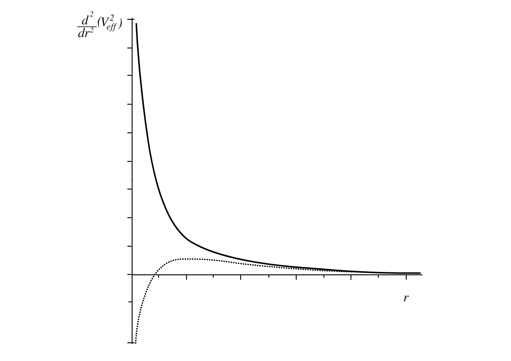
Figure 6: The condition for stability of circular orbits of particles in Schwarzschild spacetime (dotted curve) and noncommutative Schwarzschild-AdS (continuous curve). In the commutative case the condition for stability is given by $r\geq 6GM$. In the noncommutative situation the circular orbits are always stable.

IV Conclusion

In this paper we have studied the effects of noncommutativity in the orbits of particles in Schwarzschild-AdS spacetime. By means of a detailed analysis of the corresponding effective potentials for particles, we find all possible motions which are allowed by the energy levels. For radial time-like geodesics, there are some bounded trajectories (depending on the exact values of the parameters). Therefore particles not always plunges into $r=0$ from an upper distance.

For non-radial time-like geodesics, elliptical orbits are allowed as well as circular orbits. We also calculated the effect of space noncommutativity on the value of the precession of the perihelion, giving an infinity serial including the cosmological constant contribution reported in key-7 and the noncommutative terms. Although this noncommutative effect is very small, it is important since reflect the nature of spacetime structure at quantum gravity level. Therefore, the geodesic structure of this black hole presents new types of motion not allowed by the Schwarzschild spacetime. Finally, the stability of circular orbits in noncommutative Schwarzschild-AdS spacetime is discussed, showing a new behavior when compared with the commutative Schwarzchild case.

In a forthcoming paper we will discuss the null geodesic structure of the noncommutative Schwarzschild-AdS spacetime.

Acknowledgement

This work was supported by the Universidad Nacional de Colombia. Hermes Project Code 13038.

References

(1)F. Kottler. Ann. Phys. 56, 410 (1918)
(2)M. J. Jaklitsch, C. Hellaby and D. R. Matravers. Gen.
Rel. Grav. 21,941 (1989)
(3)Z. Stuchlik andP. Slany, Phys. Rev. D 69,
064001 (2004)
(4)Z. Stuchlik and S. Hledik. Acta Phys. Slov. 52,
363 (2002)
(5)J. Podolsky. Gen. Rel. Grav. 31, 1703. (1999)
(6)N. Cruz, M. Olivares and J R Villanueva. Class. Quantum
Grav. 22, 1167 (2005)
(7)M. R. Douglas and N. A. Nekrasov, Rev. Mod. Phys. 73,
977-1029. (2001)
(8)R. J. Szabo, Phys. Rept. 378, 207-299. (2003)
(9)N. Seiberg and E. Witten, JHEP 9909, 032. (1999)
(10)A. Connes and M. Marcolli, arXiv: math.QA/0601054
(11)A. Connes, J. Math. Phys. 41, 3832-3866. (2000)
(12)A. Konechny and A. Schwarz, Phys. Rept. 360,
353-465. (2002)
(13)M. Chaichian et al, Eur. Phys. J. C 29, 413-432.
(2003)
(14)A. Micu and M.M. Sheikh-Jabbari, JHEP 0101,
025. (2001)
(15)S. Benczik et al, Phys. Rev. D 66, 026003.
(2002)
(16)B. Mirza and M. Dehghani. Commun. Theor. Phys. 42,
183-184. (2004)
(17)J. M. Romero and J. D. Vergara. Mod. Phys. Lett. A
18, 1673-1680. (2003)
(18)K. Nozari and S. Akhshabi, Chaos Solitons Fractals
37, 324. (2008)
(19)K. Nozari and S. Akhshabi. Europhys. Lett. 80,
20002. (2007)
(20)A. Smailagic and E. Spallucci, J. Phys. A 36 (2003)
L467
(21)A. Smailagic and E. Spallucci, J. Phys. A 36 (2003)
L517
(22)S. Ansoldi, P. Nicolini, A. Smailagic and E. Spallucci,
Phys. Lett. B 645, 261-266. (2007)
(23)P. Nicolini, A. Smailagic and E. Spalluci, Phys. Lett.
B 632, 547-551. (2006)
(24)E. Spallucci, A. Smailagic and P. Nicolini, Phys.
Rev. D 73, 084004. (2006)
(25)P. Nicolini, J. Phys. A 38, L631-L638. (2005)
(26)P. Nicolini and G. Torrieri. JHEP 1108,
097. (2011)
(27) R. Adler, M. Bazin and M. Schiffer, Introduction
to general relativity, McGraw-Hill (1975).
(28)S. Cornbleet. Am. J. Phys. 61, 7. (1993)
(29)S. M. Carroll, An Introduction to General
Relativity: Spacetime and Geometry, Addison Wesley, 2004