Abstract

We discuss and extend recent conjectures relating partial null limits of correlation functions of local gauge invariant operators and the expectation value of null polygonal Wilson loops and local gauge invariant operators. We point out that a particular partial null limit provides a strategy for the calculation of the anomalous dimension of short twist-two operators at weak and strong coupling.

1 Introduction and discussion

Increasingly efficient perturbative computational techniques for higher-order calculations and increasingly efficient use of integrability of the worldsheet theory in $AdS_{5}\times S^{5}$ have brought about, in the last few years, remarkable progress in our understanding of ${\cal N}=4$ super-Yang-Mills (sYM) theory and have exposed unexpected and fascinating relations between a priori unrelated quantities. Such a connection, proposed in [1], links gluon scattering amplitudes with the expectation value of certain null polygonal Wilson loops in ${\cal N}=4$ sYM theory. Initially suggested at strong coupling based on the AdS/CFT correspondence, this relation was generalized and successfully tested at weak coupling [2] as well.

Correlation functions of local gauge invariant operators are natural observables in a conformal field theory such as ${\cal N}=4$ sYM theory. Two-point functions are determined by the dimension of the operators; since the latter are known, at least in principle, through use of integrability, so are the two-point functions. Apart from the dimension and $SO(3,1)\times SO(6)$ charges of operators, three point functions are determined by additional coupling-constant dependent ”structure functions” whose evaluation is less clear. It is possible to argue that, if some of the operators carry large quantum numbers, the calculation can be carried out in a semiclassical expansion [3].

Even though the axioms of conformal field theories guarantee that higher-point correlation functions are determined by the two- and three-point functions, an explicit evaluation along this line is not straightforward. It is therefore interesting to devise methods to directly evaluate them either for generic position of operators or in special limits.

It was recently suggested [4] that the duality between Wilson loops and scattering amplitudes can be extended to include certain special classes of correlation functions. More precisely, for operators in the stress tensor multiplet, the following relation should hold in the planar limit:

$$\lim_{x_{i,i+1}^{2}\to 0}\frac{\langle{\cal O}(x_{1})\dots\cal O(x_{n})\rangle}{\langle{\cal O}(x_{1})\dots\cal O(x_{n})\rangle_{0}}=\frac{\langle W_{n}\rangle^{2}_{\text{fund}}}{\langle W_{n}\rangle^{2}_{0,\text{fund}}}=\frac{A^{2}(k_{i}=x_{i}-x_{i-1},i=1,\dots,n)}{A^{2}_{\text{tree}}(k_{i}=x_{i}-x_{i-1},i=1,\dots,n)}$$ (1)

where $W_{n}$ is a null polygonal Wilson loop with corners at positions $x_{i}$ with $i=1,\dots,n$. Initially proposed as a relation between correlation functions of bosonic operators, bosonic Wilson loops and MHV amplitudes, this triality conjecture was extended to supersymmetric correlators, supersymmetric Wilson loops and generic superamplitudes [5, 6]. This relation was proven at the level of the unregularized integrand in [7, 8] and shown to hold in explicit examples [5, 6] in the presence of a dimensional regulator.

It was moreover suggested and explicitly demonstrated for four-point correlation functions though two-loop order [9] that the relation (1) is not restricted to operators in the tensor multiplet, but rather holds for more general 1/2-BPS operators, including operators with large quantum numbers.

Another class of interesting observables is provided by the correlation function of Wilson loops and local operators. Such quantities are interesting for several reasons. For example, they characterize the expansion of a Wilson loop in local operators

$$\frac{W(\gamma)}{\langle W(\gamma)\rangle}=\sum_{i}\;c_{i}(\gamma)\,O_{i}(x)~{};$$ (2)

the coefficients $c_{i}$ may be found in the obvious way in terms of the correlation function $\langle W{\cal O}_{j}(y)\rangle$ and the two-point function $\langle{\cal O}_{i}(x){\cal O}_{j}(y))$. Moreover, they may be used to factorize the expectation value of a product of two Wilson loops or, if the coefficients $c_{i}$ are known, to simply evaluate this expectation value:

$$\frac{\langle W(\gamma)W(\gamma^{\prime})\rangle}{\langle W(\gamma)\rangle\langle W(\gamma^{\prime})\rangle} = \sum_{i,j}\;c_{i}(\gamma)c_{j}(\gamma^{\prime})\,\langle{\cal O}_{i}(x)\,{\cal O}_{j}(y)\rangle$$ (3)

$$= \sum_{i}\;c_{i}(\gamma)\langle{\cal O}_{i}(x)\,W(\gamma^{\prime})\rangle$$ (4)

$$= \sum_{i,j}\;{\cal F}_{ij}(x-y)\langle W(\gamma)\,{\cal O}_{i}(x)\rangle\langle{\cal O}_{j}(y)\,W(\gamma^{\prime})\rangle\ ,$$ (5)

where ${\cal F}_{ij}(x-y)$ are the relevant conformal blocks.

A second motivation for analyzing correlation functions of Wilson loops and local operators is that, for a special choice of operator (given by the chiral Lagrangian), they contain information about the higher-loop corrections to the expectation value of the Wilson loop. This is akin to the Lagrangian insertion formalism [17] used in [9] to evaluate loop corrections to correlation functions of local operators in the null separation limit.

A generalization of the relation between correlation functions of operators and null polygonal Wilson loops was recently proposed in [16]. More precisely, starting with an $(n+1)$-point correlation function and taking the limit in which $n$ points are sequentially null-separated one should find that

$$\lim_{x_{ii+1}^{2}\to 0}\frac{\langle{\cal O}(x_{1})\cdots{\cal O}(x_{n}){\cal O}(a)\rangle}{\langle{\cal O}(x_{1})\cdots{\cal O}(x_{n})\rangle}\sim\frac{\langle W_{n}\,{\cal O}(a)\rangle}{\langle W_{n}\rangle}$$ (6)

where the expectation values on the right-hand side are taken in the fundamental representation. Non-vanishing values for both correlators, ${\langle{\cal O}(x_{1})\cdots{\cal O}(x_{n})\rangle}$ and ${\langle{\cal O}(x_{1})\cdots{\cal O}(x_{n}){\cal O}(a)\rangle}$, require that the total R-charges of the product of operators in the two correlators are zero. It therefore follows that the operator ${\cal O}(a)$ must have vanishing R-charges.^,

Generalizations of (6) are fairly straightforward to formulate. For example,

$$\lim_{x_{ii+1}^{2}\to 0}\frac{\langle{\cal O}(x_{1})\cdots{\cal O}(x_{n}){\cal O}(a_{1})\dots\cal O(a_{m})\rangle^{\text{conn}}}{\langle{\cal O}(x_{1})\cdots{\cal O}(x_{n})\rangle}\sim\frac{\langle W_{n}\,{\cal O}(a_{1})\dots\cal O(a_{m})\rangle^{\text{conn}}}{\langle W_{n}\rangle}$$ (7)

where the upper index denotes a restriction to the connected part of the correlation functions and the points $a_{j}$ with $j=1,\dots,m$ are generic. One may moreover consider a second limit in which the points in this set become sequentially null separated while remaining at generic positions with respect to the points $x_{i}$, $i=1,\dots,n$. In this limit the original correlation function equals the correlation function of two null polygonal Wilson loops.

Ratios of the type (6), (7) are good observables. Indeed, as discussed in detail in [9, 4], in the null limit correlators develop the same type of singularities as null polygonal Wilson loops. Since these divergences are located around the Wilson loop cusps or, alternatively, around the operators that are sequentially null separated, in the ratios (6) and (7) these divergences cancel out leaving behind a finite quantity, which should exhibit the symmetries of the theory. In particular, the conformal symmetry of the correlation functions should be realized. It would be interesting to understand whether the additional operator insertions in eqs. (6) and (7) have any interpretation in terms of scattering amplitudes when the operators’ position is not integrated over.

Here we will prove, to all orders in a weak coupling expansion and in the regularized theory, the first equality in equation (1) as well as equations (6) and (7) for all twist-2 operators and for a finite rank of an $SU(N)$ gauge group. We will also discuss two-field operators outside this class, containing fermions and field strengths. While not identical in details, our strategy will be similar in spirit with the eikonal line arguments used in [4, 9]; we will separate the Feynman diagrams contributing to correlation functions into classes depending on whether or not there exists R-charge flow between operators and show that certain sequences of propagators between null-separated points are equivalent to null Wilson lines. We will also show that diagrams in which there is no R-charge exchange between charged fields at null-separated points have softer singularities than if R-charge flow is present. We will then extend these arguments to larger classes of operators and also to larger classes of correlation functions, in which not all points are sequentially null-separated; we will refer to them as ”partial null limits”. We will also see that the relation between correlation functions in the null separation limit and the expectation value of null polygonal Wilson loops is not restricted to four-dimensional gauge theories but rather holds in all dimensions.

The arguments in this note point to a generalizations of (6) and (7) to limits in which any operator is null-separated from at least one and at most two other operators. In this limit a correlation function reduces to the correlation function of certain non-local operators built out of fundamental fields and open Wilson lines. Let us consider the correlator of two ${\rm Tr}[Z^{2}]$ and two ${\rm Tr}[{\bar{Z}}^{2}]$ operators at positions $x_{1},\dots,x_{4}$ in the limit $x_{12}^{2}=0=x_{34}^{2}$ and all other distances being nonzero. Denoting by

$$W(x,y)={\rm P}e^{\int_{x}^{y}A}\ ,$$ (8)

it is not difficult to see that

$$\lim_{\stackrel{{\scriptstyle\scriptstyle{x_{12}^{2}\rightarrow 0}}}{{x_{34}^{2}\rightarrow 0}}}\langle{\cal O}(x_{1}){\cal O}(x_{2}){\cal O}(x_{3}){\cal O}(x_{4})\rangle\propto\langle{\rm Tr}[Z(x_{1})W(x_{1},x_{2}){\bar{Z}}(x_{2})]{\rm Tr}[Z(x_{3})W(x_{3},x_{4}){\bar{Z}}(x_{4})]\rangle\ .$$ (9)

Clearly, the open Wilson lines are null. The proportionality coefficient depends on the regularization scheme and on the order of limits. This generalization provides a direct link between four-point correlators of BPS operators and two-point functions of non-BPS operators. Indeed, each non-local operators ${\rm Tr}[Z(x)W(x,y){\bar{Z}}(y)]$ may be expanded in twist-two operators thus reducing the four-point correlator reduces to a superposition of two-point functions. Making explicit this decomposition should allow one to read off the anomalous dimensions of twist-two operators. This approach may be particularly efficient for the lowest twist-two operators – ${\rm Tr}[Z{\bar{Z}}]$ – which is a member of the Konishi multiplet and may offer an alternative approach to the calculation of anomalous dimensions of short operators at strong coupling.

The rest of this note is organized as follows. In § 2 we discuss general features of correlation functions, define the regularization scheme and the null limit, and outline the proof of relations (1), (6) and (7). Later sections contain some of the details completing this proof. We proceed in § 3 to discuss the correlation function of 2-field scalar operators in the stress tensor multiplet in the null separation limit and identify the relevant Feynman diagrams that contribute in this limit. We then proceed in § 4 to extend the discussion in § 3 to the case of $(n+1)$-point correlation function with $n$ null-separated points. We will finish this section with comments on the more general correlators of the type mentioned in equation (7). In § 5 we discuss twist-2 operators with higher spin and extend the results described in the previous sections to their correlation functions. In § 6 we comment on other weak and strong coupling features of the correlator/Wilson loop relations. Appendix Appendix: Null separation limit for correlations of operators with gauge fields and fermions details the null and partial-null separation limit of correlation functions of two-field operators constructed from fermions and gauge fields.

2 Correlation functions in null and partial null limits

Let us consider the correlation function of some number of operators of length 2 in a gauge theory with an $SU(N)$ gauge group; we will keep $N$ arbitrary and discuss the large $N$ limit at the end. Such a correlator is symmetric under the permutation of positions of identical operators; for example, the correlation function of $n$ operators in the ${\bf 20}^{\prime}$ representation of $SO(6)$ will be symmetric under the permutation of positions of all operators. Taking the limit in which the operators are null-separated requires choosing a specific sequence of positions, e.g. $x_{1},\dots,x_{n}$ and setting $|x_{i,i+1}|^{2}\rightarrow 0$. This choice breaks their permutation symmetry to one of its cyclic subgroups ; different choices of sequences will lead, in this limit, to different dominant terms which, through the correlator/amplitude relation [9], are related to (squares of) different color-ordered amplitudes.

To take the limit in which (some) operators are null-separated it is useful to start with the momentum space correlation function and Fourier-transform it to position space. In momentum space each operator ${\cal O}_{i}$ carries nontrivial momentum —
${\widetilde{\cal O}}(q)=\int d^{d}x\exp(-iq\cdot x){\cal O}(x)$ — which is split between the fields composing it, $q_{i}=p_{i1}+p_{i2}$, as shown in fig. 1. One may arbitrarily choose a sequence of propagators connecting adjacent points; denoting this sequence by ${\tilde{L}}(p_{ij},p_{i+1,j},k)_{A}$ with $k$ the momenta of the lines attaching this sequence to the rest of the diagram and $A$ the corresponding indices, and by $G(k)_{A_{1}\dots A_{n}}$ the Green’s function obtained by removing all ${\tilde{L}}(p_{ij},p_{i+1,j},k)_{A}$, it is easy to see that

$$\langle{\widetilde{\cal O}}_{1}(q_{1})\cdots{\widetilde{\cal O}}_{n}(q_{n})\rangle=\int\prod_{i=1}^{n}\prod_{j=1}^{2}d^{d}p_{ij}[d^{d}k]\delta^{d}(q_{i}-p_{i1}-p_{i2}){\widetilde{L}}(p_{ij},p_{i+1,j},k)_{A_{i}}\;G(k)_{A_{1}\dots A_{n}}\ ,$$ (11)

where the measure factor $[d^{d}k]$ stands for integration over the momenta of all external lines of $G(k)$. The factors ${\tilde{L}}$ may contain momentum factors arising from derivatives present in operators. Fourier-transforming back to position space implies that

$$\langle{{\cal O}}_{1}(x_{1})\cdots{{\cal O}}_{n}(x_{n})\rangle=\int[d^{d}k]\prod_{i=1}^{n}\prod_{j=1}^{2}\int d^{d}p_{ij}\,{\overrightarrow{\cal D}}_{x_{i}}{L}(x_{i},x_{i+1},k)_{A_{i}}{\overleftarrow{\cal D}}_{x_{i+1}}\;G(k)_{A_{1}\dots A_{n}}\ ,$$ (12)

where ${\cal D}$ are differential operators which are present if ${\cal O}_{i}$ contain derivatives and

$${L}(x_{1},x_{2},k)_{A_{i}}=\int d^{d}p_{1}d^{d}p_{2}\,e^{ip_{1}\cdot x_{1}+ip_{2}\cdot x_{2}}\,{\widetilde{L}}(p_{1},p_{2},k)_{A_{1}}\ .$$ (13)

The presentation (12) of correlation functions is quite general and does not assume any specific structure for the operators ${\cal O}_{i}$ apart from their two-field structure. In the following we will mainly restrict to operators carrying nontrivial R-charge. By considering all possible choices of $L(x_{1},x_{2},k)$ we will identify the one that is dominant – i.e. it has the strongest singularity – in the limit $|x_{12}|^{2}\rightarrow 0$. We will moreover see that this $L(x_{1},x_{2},k)$ may be interpreted in terms of a null Wilson line with fields attached to it.

Figure 1: Presentation of a generic correlation function in terms of a Green’s function and sequences of propagators between operator insertion points which are taken to be null separated. Additional operators, which do not participate in this limit and are denoted by a heavy dot, may also be present.

While this appears to be a classical computation, it may be promoted to an all-loop one in a regularization scheme in which the (partial) null-separation limit can be decoupled from the integrals over the internal momenta $k$. Such a scheme indeed exists: it suffices to take the limit $|x_{i,i+1}|^{2}\rightarrow 0$ such that

$$|x_{i,i+1}|^{2}k^{2}\rightarrow 0$$ (14)

for all possible internal momenta $k$. With this assumption, the null separation limit can be taken at the level of the (regularized) integrand. In the following sections we will show that, in this case, a sequence of scalar propagators with gluons attached to in though three-point vertices reduces in the null separation limit to a null Wilson line with the same number of attached gluons; this yields the desired results, to all orders in weak coupling perturbation theory. As discussed in [4], in other schemes this is only a proportionality relation.

As outlined here, the arguments in the following sections focus on only two operators at a time and justify the appearance of a Wilson line between their insertion points in the limit in which they are null-separated. There arguments will also support the relation between correlation functions in the limit in which $x_{i,i+1}^{2}=0$ but $x_{i-1,i}^{2}\neq 0$ for some subset of operators and the correlation function of appropriately capped open null zig-zag Wilson lines, as illustrated in eq. (9).

3 2-field operators; no insertions

With the strategy outlined in the previous section, let us now proceed to prove the first equality (1) for charged 2-field BPS operators to all orders in perturbation theory and in the presence of a dimensional regulator. We will begin by showing that, in the limit of null separation, the diagrams exhibiting a connected R-charge flow dominate over the diagrams with disconnected flows and that the former reduce to the expectation value of a Wilson loop in the adjoint representation. Moreover, it will turn out that the dominant diagrams will contain a continuous sequence of scalar propagators.

3.1 R-charge flow through scalar exchange

Let us consider a sequence of $n$ one-gluon vertices connected by scalar propagators, as shown in fig. 2. The momenta going to the two endpoints are denoted $p_{1}$ and $p_{2}$ while the momenta carried by gluons are denoted by $k_{i}$ and the momenta of the scalars between vertices are denoted by $q_{i}$. Throughout we will not write explicitly the propagator of the gluons attached to the vertices between the points $x_{1}$ and $x_{2}$. The starting expression is thus:

$$L(x_{1},x_{2},k_{1},\cdots,k_{n})_{\mu_{1}\cdots\mu_{n}}=\int d^{d}p_{1}\int d^{d}p_{2}e^{ip_{1}\cdot x_{1}+ip_{2}\cdot x_{2}}\int d^{d}q_{1}\cdots\int d^{d}q_{n-1}$$

$$\qquad\quad\times\frac{(p_{1}-q_{1})_{\mu_{1}}(-q_{1}-q_{2})_{\mu_{2}}\cdots(-q_{n-2}-q_{n-1})_{\mu_{n-1}}(-q_{n-1}-p_{2})_{\mu_{n}}}{(p_{1}^{2}+i0)(q_{1}^{2}+i0)\cdots(q_{n-1}^{2}+i0)(p_{2}^{2}+i0)}$$ (15)

$$\times\delta^{(d)}(k_{1}+q_{1}+p_{1})\delta^{(d)}(k_{2}-q_{1}+q_{2})\cdots\delta^{(d)}(k_{n-1}-q_{n-2}+q_{n-1})\delta^{(d)}(k_{n}-q_{n-1}+p_{2})$$

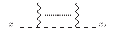
Figure 2: Contributions of scalar propagators (represented by dashed lines) and gluon-scalar vertices.

By performing all the integrals except the one over $p_{1}$, Schwinger-parametrizing the propagators and representing the factors of $p_{1}$ in the numerator as derivatives with respect to $x_{1}$ it follows that

$$L(x_{1},x_{2},k_{1},\cdots,k_{n})_{\mu_{1}\cdots\mu_{n}}=\int d^{d}p_{1}\frac{e^{ip_{1}\cdot(x_{1}-x_{2})-i\sum_{i}k_{i}\cdot x_{2}}\prod_{i=1}^{n}(2p_{1}+2\sum_{j=1}^{i-1}k_{j}+k_{i})_{\mu_{i}}}{(p_{1}^{2}+i0)\prod_{i=1}^{n}((p_{1}+\sum_{j=1}^{i}k_{j})^{2}+i0)}$$

$$\qquad\qquad={}(-i)^{(n+1)}\prod_{i=1}^{n}\left(-2i\frac{\partial}{\partial x_{1}^{\mu_{i}}}+2\sum_{j=1}^{i-1}k_{j\mu_{i}}+k_{i\mu_{i}}\right)\left(\prod_{i=1}^{n+1}\int_{0}^{\infty}d\alpha_{i}\right)e^{-i\sum_{i}k_{i}\cdot x_{2}}$$

$$\qquad\qquad\qquad\qquad\qquad\qquad\times\int d^{d}p_{1}e^{ip_{1}\cdot(x_{1}-x_{2})+i\sum_{i=1}^{n+1}\alpha_{i}(p_{1}+\sum_{j=1}^{i-1}k_{j})^{2}-0\sum\alpha_{i}}\ .$$ (16)

The change of variables $\alpha_{i}=\zeta s_{i}$ with $s_{i}\in[0,1)$, $\sum_{i=1}^{n+1}s_{i}=1$ and $\zeta\in[0,\infty)$ further simplifies this expression. Moreover, writing $s_{i}=t_{i}-t_{i-1}$ for $i=1,\dots,n$ and with $t_{0}=0$, the unit sum constraint on the $s$ variables becomes just $s_{n+1}=1-t_{n}$. Together with the evaluation of the $p_{1}$ integral, these transformations lead to:

$$L(x_{1},x_{2},k_{1},\cdots,k_{n})_{\mu_{1}\cdots\mu_{n}}=(-i)^{(n+1)}\prod_{i=1}^{n}\left(-2i\frac{\partial}{\partial x_{1}^{\mu_{i}}}+2\sum_{j=1}^{i-1}k_{j\mu_{i}}+k_{i\mu_{i}}\right)$$ (17)

$$\quad\times\left(\prod_{i=1}^{n}\int_{t_{i-1}}^{1}dt_{i}\right)e^{-i\sum_{i}k_{i}\cdot(x_{2}t_{i}-x_{1}(1-t_{i}))}\int_{0}^{\infty}d\zeta\zeta^{n}\frac{\pi^{2-\epsilon}}{(-i\zeta)^{2-\epsilon}}e^{i\zeta\tilde{f}(t_{i},k_{i})-i\frac{(x_{1}-x_{2})^{2}}{4\zeta}-0\zeta-0/\zeta}\ ,~{}$$

with some functions $\tilde{f}(t_{i},k_{i})$ whose expressions are not important.

The integral over $\zeta$ is of the general type

$$I_{m}(z,f)=\int d\zeta\;\zeta^{m-2+\epsilon}e^{i\zeta f-i\frac{z^{2}}{\zeta}-0\zeta-0/\zeta}$$ (18)

with some choice of $m$ and with some function $f$ depending on the momenta $k_{i}$ and the affine parameters $t_{i}$; such integrals will also appear in later sections in diagrams involving other types of fields. The rescaling $\zeta\rightarrow\zeta z^{2}$ together with the null-separation limit implies that

$$\lim_{z^{2}\to 0}I_{m}(z,f)=(-1)^{\frac{1-m-\epsilon}{2}}\Gamma(1-m-\epsilon)z^{2(m+\epsilon-1)}$$ (19)

for $m\leq 0$. For $m\geq 1$ the integral does not vanish, but reduces to an $f$-dependent (and $z$-independent) constant.

The leading term in the light-like limit arises from the highest power of $\zeta^{-1}$ brought down by the differentiation with respect to $x_{1}$. It is easy to see that it is $\zeta^{-n}$; this factor cancels the $\zeta^{n}$ measure factor arising form the change of variables and leaves behind an $n$-independent $\zeta$ factor which generates, upon integration, a factor of the position space scalar propagator $\Delta_{4-2\epsilon}(x_{1}-x_{2})$. The remaining integral represents $n$ correctly ordered Wilson line vertices together with the exponential factors needed to Fourier-transform the gluon propagator:

$$L(x_{1},x_{2},k_{1},\cdots,k_{n})_{\mu_{1}\cdots\mu_{n}}$$ (20)

$$\qquad\qquad=\Delta_{4-2\epsilon}(x_{1}-x_{2})\,\prod_{i=1}^{n}\;i(x_{1}-x_{2})_{\mu_{i}}\;\int_{t_{i-1}}^{1}dt_{i}\;e^{-i\sum_{i}k_{i}\cdot(x_{2}t_{i}-x_{1}(1-t_{i}))}~{},~{}~{}~{}~{}$$ (21)

where, as mentioned before, $t_{0}=0$. We have therefore recovered, in the scheme used here, the results of the eikonal approximation: a continuous sequence of scalar propagators connecting two operators that become light-like separated is equivalent to a light-like Wilson line between the operators’ positions. 

The derivation described above points to a simple rule for identifying the diagrams that survive in the light-like limit: once all propagators are written with standard $(p^{2}+i0)$ denominators, one simply counts the number of momentum factors of lines connecting the two insertion points. If this number is equal to the number of propagators minus one, then the corresponding diagram yields a sufficiently singular contribution. Otherwise it drops out in the null separation limit.

For this reason the four-point gluon-scalar interaction cannot contribute to the leading term in the null-separation limit: since such a vertex has no derivatives, replacing a three-point vertex in eq.(15) with one such vertex would lead to an eq. (17) with one fewer derivative factor and hence to an extra factor of $\zeta$ in the integral. It will therefore not be sufficiently singular to contribute in the limit in which R-charge flows between light-like separated points.

3.2 Other interactions leading to R-charge flow

Apart from a continuous sequence of scalar propagators, R-charge flow between two operators may be realized by a sequence of scalars and fermions. We illustrate this possibility in fig. 3 with two scalars and any number of fermions; the sequence of fermion propagators may also be interrupted by further scalar lines, in which case more of the open-ended lines become scalars.

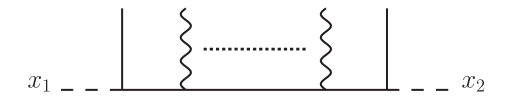
Figure 3: An example of diagram exhibiting R-charge flow which is subleading in the null-separation limit. Dashed lines represent scalar fields while solid lines represent fermions.

The relation between the singularity in the null separation limit and the structure of the momentum dependence of the integrand of the Fourier transform of such a sequence suggests that, for a fixed number of propagators, the most singular terms arise from the terms with the highest number of momentum factors in the numerator. This illustrates the importance of the spin of the exchanged particle in the null-separation limit. Since no derivatives appear in the interaction of fermions and scalars and of fermions and gluons, the only source of numerator momenta in fig. 3 is the numerator of fermion propagators. Consequently, the diagrams with more than the two scalar propagators will have a softer singularity than the diagram shown in this figure. Let us then discuss the situation of the highest number of fermion propagators — $(n-2)$ for a total of $n$ lines. The relevant Fourier-transform is

$$L(x_{1},x_{2},k_{1},\cdots,k_{n})_{\mu_{1}\cdots\mu_{n-2}}$$ (23)

$$= \int d^{d}p_{1}\int d^{d}p_{2}e^{ip_{1}\cdot x_{1}+ip_{2}\cdot x_{2}}\int d^{d}q_{1}\dots\int d^{d}q_{n-1}\frac{q\hbox to0.0pt{\hss/}{}_{n-1}\gamma_{\mu_{n-2}}\dots q\hbox to0.0pt{\hss/}{}_{2}\gamma_{\mu_{1}}q\hbox to0.0pt{\hss/}{}_{1}}{(p_{1}^{2}+i0)(q_{1}^{2}+i0)\dots(q_{n-1}^{2}+i0)(p_{2}^{2}+i0)}$$

$$\times\delta^{(d)}(k_{1}+q_{1}+p_{1})\delta^{(d)}(k_{2}-q_{1}+q_{2})\cdots\delta^{(d)}(k_{n-1}-q_{n-2}+q_{n-1})\delta^{(d)}(k_{n}-q_{n-1}+p_{2})~{}.~{}~{}$$

Carrying out the $q$ integrals, Schwinger-parametrizing the resulting propagators and changing variables as discussed in the previous section leads to an expression of the type

$$L(x_{1},x_{2},k_{1},\cdots,k_{n})_{\mu_{1}\cdots\mu_{n-2}}$$ (25)

$$\sim \left[\prod_{j=1}^{n-1}\frac{\partial}{\partial x_{1}^{\sigma_{j}}}+{\rm fewer~{}derivatives}\right]\left(\prod_{i=1}^{n}\int_{t_{i-1}}^{1}dt_{i}\right)e^{-i\sum_{i}k_{i}\cdot(x_{2}t_{i}-x_{1}(1-t_{i}))}$$

$$\qquad\times T^{\sigma_{n-1}\mu_{n-2}\dots\mu_{1}\sigma_{1}}\int_{0}^{\infty}d\zeta\zeta^{n}\frac{\pi^{2-\epsilon}}{(-i\zeta)^{2-\epsilon}}e^{i\zeta\tilde{f}(t_{i},k_{i})-i\frac{(x_{1}-x_{2})^{2}}{4\zeta}-0\zeta-0/\zeta}~{}~{},$$

where $T$ is a product of Dirac matrices. It is easy to see that, among the integrals defined in (18), only $I_{m}$ with $m\geq 1$ can appear from the action of derivatives. As expected, it follows from (19) that all such diagrams are not sufficiently singular in the limit of null separation and thus can be ignored.

It is clear that a similar argument goes through if some of the fermion lines are replaced with scalar lines; such contributions can also be ignored.

3.3 No R-charge flow between two insertion points

The typical diagram that does not exhibit R-charge flow between two charged operators involves at least one gluon propagating along any possible path between them – see fig. 4. The sequence of gluon propagators may be interrupted by scalar or fermion lines. Since the fermion-gluon interaction has no derivatives, the discussion in the previous section implies that such diagrams are not sufficiently singular in the null-separation limit and we can ignore them. We will therefore focus on gluons and scalars and, for the same reason as above, also ignore the four-point interactions.

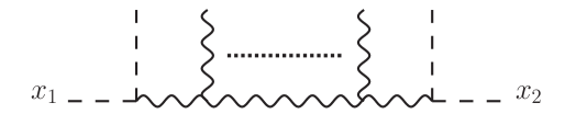
Figure 4: Example of contributions without R-charge flow between two operators.

The momentum dependence of the gluon-scalar three-point vertices guarantees that Feynman diagrams of the type shown in fig. 4 have the correct momentum dependence to potentially yield leading order contributions in the limit of null separation of insertion points; this would be the case if, upon Fourier transform, each vertex contributes a factor of $(x_{1}-x_{2})^{\mu}$. Such a relation also appeared in § 3.1. A closer inspection reveals however that these potentially dangerous diagrams do not contribute. To see this let us assume that there are $n$ vertices and $(n+1)$ propagators between insertion points. Of the external lines not attached to the insertion points, at least two are scalars, leaving only at most $(n-2)$ outgoing gluon lines and consequently at most $(n-2)$ free Lorentz indices. Since there are $n$ factors of $(x_{1}-x_{2})^{\mu}$, one for each vertex, it immediately follows that at least two such factors are necessarily contracted (otherwise there would be more than $n-2$ free indices) and at least one more $(x_{1}-x_{2})^{2}$ numerator factor is generated.

Since the Feynman diagrams contributing to fig. 4 depend on a number of additional vectors – e.g. the momenta of external particles – one may wonder whether two of the indices arising from the $n$ vertices may be contracted with such vectors rather than produce an $(x_{1}-x_{2})^{2}$. Such contributions can be ruled out by noticing, on the one hand dimensional analysis requires that the number of numerator factors be fixed and on the other factors of external momenta lower the singularity through the absence of $\zeta^{-1}$ factors.

It therefore follows that, regardless of the mechanism that is responsible for the reduction of the number of free vector indices – either contraction with some $k_{i}$ or the appearance of an explicit $(x_{1}-x_{2})^{2}$ factor – the null separation limit $(x_{1}-x_{2})^{2}\rightarrow 0$ contains no singularities. This completes the proof that, if a connected R-charge flow can exist between scalar operators, then only Feynman diagrams leading to this flow contribute in the null separation limit.

We have therefore shown that, in the presence of a dimensional regulator and in the scheme described in § 2, the correlation function of length-2 scalar operators in the null separation limit is proportional to the expectation value of a null polygonal Wilson loop in the adjoint representation with cusps at the positions of the original operators:

$$\langle{\cal O}(x_{1})\cdots{\cal O}(x_{n})\rangle=\langle W_{n}\rangle_{\text{adj}}\;\prod_{i=1}^{n}\Delta(x_{i}-x_{i+1})~{}.$$ (26)

In general, as explained in [4, 9], a scheme-dependent coefficient function will appear on the right-hand side of this equation and will capture the differences between different possible light-like limits and their inter-relation with the regulator. The arguments presented here hold for finite values of the rank of the gauge group and do not rely on the existence of supersymmetry. Our proof extends the arguments of [7] to the regularized theory. We will comment in the Appendix on correlation functions of operators built from other fields.

4 2-field operators and additional operator insertions

Let us now proceed to discuss more general limits of correlation functions, in which only a subset of operators participate in the null separation limit.

4.1 A single additional operator

Let us first consider the correlation functions of $n+1$ operators, $n$ of which participate in the null separation limit. The additional operator ${\cal O}(a)$ is located at a generic position, $(x_{i}-a)^{2}\neq 0$ for all $i=1,\cdots,n$. As discussed in the Introduction, such an operator should have vanishing R-charge, otherwise a nonvanishing correlation function $\langle{\cal O}(x_{1})\cdots{\cal O}(x_{n})\rangle$ implies that $\langle{\cal O}(x_{1})\cdots{\cal O}(x_{n}){\cal O}(a)\rangle=0$.

The arguments in the previous section apply equally well if the additional operator does not affect the R-charge flow between two light-like separated operators. Indeed, if ${\cal O}(a)$ is connected to the scalar and/or fermion lines as in fig. 5(a) and 5(b), then it acts similarly to any other multi-point interaction arising from the Lagrangian: the continuous sequence of scalar propagators will continue to dominate in the presence of an additional operator insertion. A similar conclusion – that the presence of the additional operator does not affect the conclusion of the previous section – can be reached if the operators is inserted in the diagrams in fig. (4) while being attached to some of the fields denoted by open lines – see fig. 5(c). Dimensional arguments also imply that diagrams that are subleading in the absence of the additional operator cannot acquire a stronger singularity.

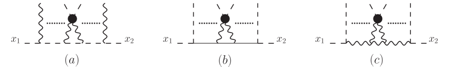
Figure 5: Example of diagrams in which the additional operator (denoted by a heavy dot) acts as a Lagrangian interaction vertex.

The other possible way of inserting the additional operator is by interrupting the sequence of propagators explicitly shown in figs. 2, 3 and 4, as illustrated in fig. 6 for the Feynman diagrams dominant in the null separation limit. One may intuitively expect that, since the insertion point $a$ is not null-separated from $x_{1}$ and $x_{2}$, the limit $(x_{1}-x_{2})^{2}\rightarrow 0$ is non-singular. A short calculation shows that this is indeed the case; we shall illustrate it with the example of an operator ${\cal O}(a)$ with arbitrary number of derivatives inserted in a continuous sequence of scalar propagators.

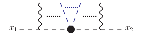
Figure 6: An operator insertion (denoted by a heavy dot) along an R-charge flow. Since the insertion point is not integrated over, the limit $(x_{1}-x_{2})^{2}\rightarrow 0$ is non-singular.

Assuming that the operator is inserted at position $a$, that the fields that are Wick-contracted with the scalars in the original sequence of propagators carry $n_{1}$ and $n_{2}$ derivatives and using $L(x_{1},x_{2},k)_{\mu_{1}\cdots\mu_{n}}$ in eq (17) it is easy to see that fig. 6 will contribute the following to the correlation function of the $n+1$ operators:

$$L(x_{1},a,x_{2},k_{1},\cdots,k_{n},O^{\prime})_{\mu_{1}\cdots\mu_{n}}$$ (27)

$$= (\partial_{a})^{n_{1}}L(x_{1},a,k_{1},\cdots,k_{r})_{\mu_{1}\cdots\mu_{r}}\;{{\widetilde{O}}^{\prime}(a)}\;(\partial_{a})^{n_{2}}L(a,x_{2},k_{r+1},\cdots,k_{n})_{\mu_{r+1}\cdots\mu_{n}}\ ,$$ (28)

where $(\partial_{a})^{n_{1}}$ and $(\partial_{a})^{n_{1}}$ stand for products of derivatives with potentially suppressed free indices and ${{\widetilde{O}}^{\prime}}$ contains the fields of ${\cal O}(a)$ that are not contracted with the scalar line. Neither one of the two $L$ factors is singular as $(x_{1}-x_{2})^{2}\rightarrow 0$. It therefore follows that these terms, as well as the others obtained by replacing some or all of the scalars with gluons and/or fermions give subleading contributions compared to the Feynman diagrams in which $O$ is not interrupting the sequence of scalar propagators connecting two light-like separated points.

Thus, in the limit in which $x_{i}$ with $i=1,\dots,n$ are sequentially null separated, the correlator $\langle O(x_{1})\cdots O(x_{n})O(a)\rangle$ becomes proportional to the correlation function of the null Wilson loop in the adjoint representation with corners at positions $x_{i}$ and the additional operator ${\cal O}(a)$.

4.2 Several additional operators

It is not difficult to generalize the arguments in the previous section to the insertion of several operators which are placed at generic positions relative to the points $x_{i}$ with $1\dots n$. In such case the only constraint stemming from R-charge conservation is that the total charge of the insertions vanishes: $\sum_{j=1}^{M}Q_{R}({\cal O}(a_{m}))=0$.

If none of the operators interrupts the R-charge flow between two null-separated operators they act, as in the case of a single operator insertion, as a Lagrangian interaction vertex. If a sequence of scalar propagators is interrupted by an additional operator then it becomes non-singular in the limit in which its beginning and end points are null separated. It therefore follows that

$$\lim_{x_{ii+1}^{2}\to 0}\frac{\langle{\cal O}(x_{1})\cdots{\cal O}(x_{n}){\cal O}(a_{1})\cdots{\cal O}(a_{m})\rangle^{\text{conn}}}{\langle{\cal O}(x_{1})\cdots{\cal O}(x_{n})\rangle}=\frac{\langle W_{n}\,{\cal O}(a_{1})\cdots{\cal O}(a_{m})\rangle^{\text{conn}}}{\langle W_{n}\rangle}~{}~{}.$$ (29)

As before, the Wilson loop is in the adjoint representation and the upper index denotes the fact that on both sides of this equation one should restrict to the connected part of the correlation functions. Relaxing this constraint will replace the right-hand side numerator with a sum over connected components, each of which being the product of the correlation function of $W_{n}$ and some subset of ${\cal O}(a_{1})\dots\cal O(a_{m})$ and the correlation function of the remaining operators.

For sufficiently many additional operator insertions one may take a further limit, in which $(a_{j}-a_{j+1})^{2}\rightarrow 0$ but at generic positions compared to $x_{i}$. Dividing by $\langle{\cal O}(a_{1})\cdots{\cal O}(a_{m})\rangle$ it then follows that

$$\lim_{\stackrel{{\scriptstyle\scriptstyle{x_{ii+1}^{2}\to 0}}}{{\scriptstyle{a_{jj+1}^{2}\to 0}}}}\frac{\langle{\cal O}(x_{1})\cdots{\cal O}(x_{n}){\cal O}(a_{1})\cdots{\cal O}(a_{m})\rangle}{\langle{\cal O}(x_{1})\cdots{\cal O}(x_{n})\rangle\langle{\cal O}(a_{1})\cdots{\cal O}(a_{m})\rangle}=1+\frac{\langle W_{n}\,W_{m}\rangle_{\text{adj}}^{\text{conn}}}{\langle W_{n}\rangle\langle W_{m}\rangle_{\text{adj}}}\ .$$ (30)

As before, the upper index on the right-hand side denotes a restriction to the connected part of that correlator; the constant term is the contribution of one of the disconnected components of $\langle{\cal O}(x_{1})\cdots{\cal O}(x_{n}){\cal O}(a_{1})\cdots{\cal O}(a_{m})\rangle$. The other disconnected components have a different singularity structure and their contribution to the ratio (30) vanishes in the null separation limit.

One may consider the factorization of the correlation function of Wilson loops, as outlined in eq. (5). From the perspective of eq. (30), it corresponds to a particular factorization of the correlation function of $n+m$ operators into the sum of products of $n+1$ and $m+1$-point correlation functions.

4.3 Large $N$ limit

The arguments described above are independent of the rank of the $SU(N)$ gauge group. To make contact with a strong coupling analysis it is necessary to consider the large-$N$ limit. In the absence of operator insertions this limit is standard

$$\lim_{N\to\infty}\langle W_{n}\rangle_{\text{adj}}=\langle W_{n}\rangle_{\text{fund}}^{2}\ .$$ (31)

Diagrammatically, this relation arises from the fact that the Feynman diagrams of the type shown in fig. (7)(a) are subleading in the large $N$ limit compared to diagrams in figs. (7)(b). The graph in fig. 7(c) may or may not contribute depending on the rest of the diagram. That is, the only Feynman diagrams that survive in this limit are those in which the inner and outer index lines of the Wilson loop are connected to themselves by some webs of vertices and propagators from the Lagrangian. Moreover, away from the Wilson loop, the Feynman diagram is planar.

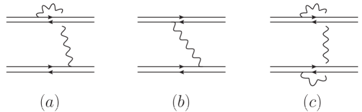
Figure 7: Leading and subleading diagrams in the large-$N$ limit. The double-lines denote Wilson lines and the wavy line represent gluons.

It is not difficult to generalize this picture to the correlation function of a Wilson loop and an operator, $\langle W_{n}{\cal O}(a)\rangle_{\text{adj}}$. The Feynman diagrams that survive the large-$N$ limit are those in which the operator ${\cal O}(a)$ is connected only to one index line of the Wilson loop. Thus,

$$\lim_{N\to\infty}\langle W_{n}\,{\cal O}(a)\rangle_{\text{adj}}=2\langle W_{n}\rangle_{\text{fund}}\langle W_{n}{\cal O}(a)\rangle_{\text{fund}}\ .$$ (32)

The factor of $2$ arises because the operator may be connected either to the inner of the outer index line (e.g. it may be inserted on the gluon line in figs. (7)(b) and (c)). This factor is in agreement with the discussion in [16] on the insertion of the (integrated) dilaton vertex operator.

Following a similar reasoning it is easy to take the planar limit for the correlator of a Wilson loop and several operators. The Feynman graphs can be organized into sets of diagrams in which some operators are connected to one Wilson loop index line and the other operators are connected to the other Wilson loop index in a planar way, i.e.

$$\lim_{N\to\infty}\langle W_{n}\,{\cal O}(a_{1})\cdots{\cal O}(a_{m})\rangle_{\text{adj}}$$

$$= \sum_{k=0}^{m}\sum_{\{j_{1},\dots,j_{k}\}\subset\{1,\dots,m\}}\langle W_{n}\,{\cal O}(a_{j_{1}})\cdots{\cal O}(a_{j_{k}})\rangle_{\text{fund}}\langle W_{n}\,{\cal O}(a_{j_{k+1}})\cdots{\cal O}(a_{j_{m}})\rangle_{\text{fund}}\ ,$$

where the second sum runs over all subsets of $\{1,\dots,m\}$ with $k$ elements. If the total R-charge of the operators appearing in an expectation value is nonzero, $\sum_{l=1}^{k}R({\cal O}(x_{j_{l}}))\neq 0$, the corresponding term vanishes identically. For example, if $m=2$ the R-charges of the two operators must be equal in absolute value; if their common value is nonvanishing, then all correlators involving one Wilson loop and one operator vanish identically and, in the sum above, only the terms with $k=0$ and $k=m=2$ survive.

Last, the factorization of the connected part of the correlation function of two Wilson loops follows a similar pattern:

$$\lim_{N\to\infty}\langle W_{n}W_{m}\rangle^{\text{conn}}_{\text{adj}}=2\langle W_{n}\rangle_{\text{fund}}\langle W_{m}\rangle_{\text{fund}}\langle W_{n}W_{m}\rangle^{\text{conn}}_{\text{fund}}\ .$$ (34)

This term arises form the $k=0$ and $k=m$ terms in eq. (4.3). The other terms disappear in the null limit because there is no R-charge flow between operators (in fact there are no fields that propagate between the operators in one set and the operators in the other) and thus are subleading compared to eq. (34).

5 Operators with higher spin

As reviewed in § 1, it was suggested in [4] that the relation between correlation functions and Wilson loops is not restricted to the operators in the stress tensor multiplet. If such a generalization is indeed correct, it is tempting to expect that it would hold in the presence of additional insertions as well. Such a generalization, both in the absence and in the presence of additional operator insertions, is potentially very interesting. A relation between correlation functions and Wilson loops suggests that, at least in the null separation limit and at string coupling, correlation functions should have a semiclassical description. While such an approach is difficult to justify for operators of small dimension (even in the null separation limit), a justification is readily available [3] for operators whose dimension scales like $\Delta\propto\sqrt{\lambda}$.

5.1 No additional insertions

The discussion in the previous sections can be extended without much difficulty to the case when the operators inserted at positions $x_{1},\cdots,x_{n}$ are twist-2 operators

$${\cal O}^{S}=\sum_{n=0}^{S}\,c_{n}(\lambda){\rm Tr}[D_{+}^{n}ZD_{+}^{S-n}Z]\ ,$$ (35)

where the coefficients $c_{n}(\lambda)$ are determined by requiring that these operators have definite anomalous dimensions. At one loop, they are given [21] in terms of the Jacobi polynomials

$${\cal O}^{S}=i^{s}(n\cdot D_{1}+n\cdot D_{2})^{S}P_{S}^{(0,0)}\left(\textstyle{\frac{n\cdot D_{2}-n\cdot D_{1}}{n\cdot D_{2}+n\cdot D_{1}}}\right){\rm Tr}[Z(\xi_{2})Z(\xi_{1})]\Big{|}_{\xi_{1}=\xi_{2}}\ ,$$ (36)

where $n\cdot D$ are covariant derivatives in the adjoint representation in the light-like direction specified by the vector $n$. Our regularization scheme implies however that the following arguments hold even if ${\cal O}^{S}$ does not have definite anomalous dimension.

As we saw in the previous sections, in the null separation limit, the Feynman diagrams that dominate the correlation function of 2-field scalar operators generate R-charge flow between insertion points and contribute the scalar propagator $\Delta(x_{1}-x_{2})$ multiplied by a Wilson line stretched between $x_{1}$ and $x_{2}$, see eq. (17). The additional derivatives present in the operators (35) act either on the scalar propagator prefactors $\Delta(x_{i}-x_{i+1})$ or on the Wilson line factor in the usual way:

$$\langle(n\cdot D)^{p}Z(x_{1})(n\cdot D)^{m}Z(x_{2})\rangle\mapsto(n\cdot D_{x_{1}})^{p}(n\cdot D_{x_{2}})^{m}\langle Z(x_{1})Z(x_{2})\rangle\ .$$ (37)

The derivative action on $\Delta(x_{i}-x_{i+1})$ yields terms that are more singular than $\Delta(x_{i}-x_{i+1})$. Since the action of derivatives on the Wilson line does not generate any $1/(x_{i}-x_{i+1})^{2}$ singularities, it follows that the most singular term in the null separation limit arises solely from all derivatives acting on the scalar propagator prefactors:

$$\lim_{x_{i,i+1}\to 0}\langle{\cal O}^{S_{n}}(x_{n})\cdots{\cal O}^{S_{1}}(x_{1})\rangle = \langle W_{n}\rangle\sum_{m_{1}=0}^{S_{1}}\cdots\sum_{m_{n}=0}^{S_{n}}c_{m_{1}}\cdots c_{m_{n}}\prod_{i=1}^{n}{\overleftarrow{n\cdot\partial}}_{x_{i}}{\overrightarrow{n\cdot\partial}}_{x_{i}}\Delta(x_{i}-x_{i+1})$$ (38)

$$+(\text{contributions of the gauge fields in covariant derivatives})$$

where $x_{n+1}\equiv x_{1}$ and the left derivative with respect to $x_{1}^{+}$ in the first term acts on the $\Delta(x_{n}-x_{1})$ factor.

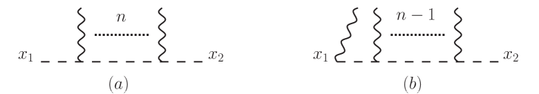
Figure 8: Contribution of the gauge field inside the covariant derivative $(b)$ compared to the contribution of a scalar line with the same number of external gluons $(a)$.

The contribution of the gauge fields present in the covariant derivatives can be shown to also be subleading. To understand this it is useful to interpret the $[A,Z]$ term in the covariant derivative as a standard $AZ{\bar{Z}}$ vertex from which one strips off the derivative. Thus, for the purpose of understanding the $x_{12}^{2}$ dependence of the gauge field contribution, we may simply analyze the expression in eq. (15) without the $1/p_{1}^{2}$ propagator and without the momentum contribution of the first gluon-scalar vertex – see fig. 8(b). It is useful to recall that the final $(x_{1}-x_{2})$ dependence is governed by the power of $\zeta$ in equation (17); there, $\zeta^{n}$ in the measure arose from the propagators and each derivative generates a factor of $\zeta^{-1}$. Thus, the two diagrams in fig. 8 will have identical singularities in the $(x_{1}-x_{2})^{2}\to 0$ limit. This singularity however is softer than that of the diagram in which the derivative acts on the scalar field; consequently, we may ignore the contribution of the gauge fields in the covariant derivatives. Thus, eq. (38) reduces to

$$\lim_{x_{i,i+1}\to 0}\langle{\cal O}^{S_{1}}(x_{1})\cdots{\cal O}^{S_{n}}(x_{n})\rangle=\langle W_{n}\rangle\sum_{m_{1}=0}^{S_{1}}\cdots\sum_{m_{n}=0}^{S_{n}}c_{m_{1}}\cdots c_{m_{n}}\prod_{i=1}^{n}{\overleftarrow{n\cdot\partial}}_{x_{i}}{\overrightarrow{n\cdot\partial}}_{x_{i}}\Delta(x_{i}-x_{i+1})\ .$$ (39)

5.2 Additional operator insertions

It is straightforward to extend the arguments above, along the lines of § 4, to the correlation function of $n+1$ operators, $n$ of which are taken to be null separated. We find

$$\lim_{x_{i,i+1}\to 0}\langle{\cal O}^{S_{1}}(x_{1})\cdots{\cal O}^{S_{n}}(x_{n}){\cal O}^{S_{a}}(a)\rangle=\langle W_{n}\,{\cal O}^{S_{a}}(a)\rangle_{\text{adj}}$$ (40)

$$\qquad\qquad\qquad\qquad\qquad\qquad\times\sum_{m_{1}=0}^{S_{1}}\cdots\sum_{m_{n}=0}^{S_{n}}c_{m_{1}}\cdots c_{m_{n}}\prod_{i=1}^{n}{\overleftarrow{n\cdot\partial}}_{x_{i}}{\overrightarrow{n\cdot\partial}}_{x_{i}}\Delta(x_{i}-x_{i+1})\ .$$

Normalizing this expression to the correlation function of the $n$ null-separated operators it follows immediately that

$$\lim_{x_{i,i+1}^{2}\to 0}\frac{\langle{\cal O}^{S_{1}}(x_{1})\cdots{\cal O}^{S_{n}}(x_{n}){\cal O}^{S_{a}}(a)\rangle}{\langle{\cal O}^{S_{1}}(x_{1})\cdots{\cal O}^{S_{n}}(x_{n})\rangle}=\frac{\langle W_{n}\,{\cal O}^{S_{a}}(a)\rangle_{\text{adj}}}{\langle W_{n}\rangle_{\text{adj}}}\ .$$ (41)

For several operator insertions at generic positions one finds for the connected part of the correlation function that

$$\lim_{x_{i,i+1}\to 0}\frac{\langle{\cal O}^{S_{1}}(x_{1})\cdots{\cal O}^{S_{n}}(x_{n}){\cal O}^{S_{a_{1}}}(a_{1})\dots\cal O^{S_{a_{m}}}(a_{m})\rangle^{\text{conn}}}{\langle{\cal O}^{S_{1}}(x_{1})\cdots{\cal O}^{S_{n}}(x_{n})\rangle}$$ (42)

$$\hskip 227.62204pt=\frac{\langle W_{n}\,{\cal O}^{S_{a_{1}}}(a_{1})\dots\cal O^{S_{a_{m}}}(a_{m})\rangle_{\text{adj}}^{\text{conn}}}{\langle W_{n}\rangle_{\text{adj}}}\ ,$$

in close analogy with the correlation function of two-field BPS operators.

6 Remarks

Let us comment here on correlation functions of higher-twist operators. In [9] it was suggested and demonstrated through two loops for four-point correlators, that the relation between correlation functions and null polygonal Wilson loops is not restricted to two-field BPS operators or, more generally, operators in the stress tensor multiplet. To see this in the regularization scheme we employed here let us consider operators connected by two or more non-overlapping sequences of propagators allowing for R-charge flow. Following the discussion in § 3, in the limit in which the two operators are null-separated, each such sequence is equivalent to a Wilson line multiplied by a position space scalar. Moreover, we have also seen that if fields other than gluons are attached to the Wilson line, the singularity of the scalar propagator is softened.

The same holds if two Wilson lines between the same two null-separated points are connected by a gluon. Indeed, since the interaction vertex between a Wilson line and a gluon is proportional to $x_{12}^{\mu}$, a gluon of this type necessarily yields a factor of $|x_{12}|^{2}$ which softens the singularity of the scalar propagator. We therefore conclude that, if two operators are connected by more than one R-charge carrying sequence of propagators, the leading contribution to the null separation limit comes from Feynman graphs in which no field connects two such sequences. This in turn implies that, in the planar limit,

$$\lim_{x_{i,i+1}^{2}\to 0}\frac{\langle{\cal O}^{J_{1}}(x_{1})\dots\cal O^{J_{n}}(x_{n})\rangle}{\langle{\cal O}^{J_{1}}(x_{1})\dots\cal O^{J_{n}}(x_{n})\rangle_{0}}=\frac{\langle W_{n}\rangle^{2}_{\text{fund}}}{\langle W_{n}\rangle^{2}_{0,\text{fund}}}$$ (43)

where ${\cal O}^{J_{i}}(x_{i})$ stands for a scalar operator with $J_{i}$ fields. In general, an additional scheme-dependent factor may appear on the right-hand side above. Unlike the two-field scalar operators however, the argument above breaks down for a finite rank gauge group.

This argument goes through unmodified if additional operators, placed at arbitrary positions, are present in the correlation function. Indeed, as discussed in previous sections, if any of the additional operators affect the R-charge flow between the null-separated ones, the resulting Feynman diagram will have a subleading singularity. In the diagrams in which the additional operators act as regular interaction vertices, the null separation limit proceeds as if they were absent, implying that

$$\lim_{\stackrel{{\scriptstyle\scriptstyle{x_{ii+1}^{2}\to 0}}}{{N\rightarrow\infty}}}\frac{\langle{\cal O}^{J_{1}}(x_{1})\cdots{\cal O}^{J_{n}}(x_{n}){\cal O}(a_{1})\cdots{\cal O}(a_{m})\rangle^{\text{conn}}}{\langle{\cal O}^{J_{1}}(x_{1})\cdots{\cal O}^{J_{n}}(x_{n})\rangle}$$ (44)

$$=\frac{1}{\langle W_{n}\rangle_{\text{fund}}^{2}}\sum_{k=0}^{m}\sum_{\{j_{1},\dots,j_{k}\}\subset\{1,\dots,m\}}\langle W_{n}\,{\cal O}(a_{j_{1}})\cdots{\cal O}(a_{j_{k}})\rangle_{\text{fund}}\langle W_{n}\,{\cal O}(a_{j_{k+1}})\cdots{\cal O}(a_{j_{m}})\rangle_{\text{fund}}\ .$$

Similarly to the partial null-separation limit of correlation functions of two-field operators (29), we expect that the scheme-dependent coefficient functions arising both in the numerator and denominator of the left-hand side of this equation cancel each other out.

While the weak coupling arguments for the relation between correlation functions and null polygonal Wilson loops are relatively straightforward, a detailed derivation of this relation remains mysterious from a strong coupling perspective. Moreover, as already mentioned in [16] for two additional operators, if the charges and dimensions of the local operators are not large enough to invalidate the semiclassical expansion, the correlation function between a Wilson loop and some number of local operators – such as the one on the right-hand side of eq. (7) – factorizes as

$$\langle W_{n}{\cal O}_{1}(a_{1})\dots\cal O_{m}(a_{m})\rangle_{\text{fund}}\rightarrow\prod_{j=1}^{m}\langle W_{n}{\cal O}_{j}(a_{j})\rangle_{\text{fund}}\ .$$ (45)

If the operators ${\cal O}_{j}$ are the gauge theory dual of the integrated dilaton vertex operators (i.e. they are the ${\cal N}=4$ action), a relation of this type can be understood at weak coupling [22, 23] by simply representing [24] ${\cal O}_{j}$ as $\lambda d/d\lambda$. One may also expect that a similar relation may hold if the integrals over the positions of the operators are omitted. It is however not immediately clear how to understand such a relation if the operators ${\cal O}_{j}$ are other BPS operators; it would be interesting to explore the origin and limitations of such a factorization at weak coupling.

Since the arguments discussed in § 3 build the closed null polygonal Wilson loops one side at a time, they can be used to also prove the relation (9) and its generalization to higher-point correlation functions and correlation function of open null zig-zag Wilson lines with arbitrary number of cusps. Such relations may provide a semiclassical approach complementary to that of [25, 26] to the calculation of anomalous dimensions of short operators, in particular of members of the Konishi multiplet.

In this note we discussed in detail the relation between the null and partial null limits of correlation functions and the expectation value of null polygonal Wilson loops as well as the correlation functions of such Wilson loops and local gauge invariant operators. Twistor space techniques were used in [27] to construct a recursion relation for the expectation value of null polygonal Wilson loops; this recursion relation mirrors that of the unregularized integrand of scattering amplitudes proposed in [28]; see also ref. [29]. The two structurally different terms arise from the self-intersections of the Wilson loop due to a BCFW-type deformation and from a quantum term in the loop equation, respectively (see [27] for details). Through the construction in [7] a similar recursion relation holds for correlation functions of gauge invariant operators in the null-separation limit. It would be interesting to investigate the existence of similar recursion relations for partial null-limits of correlation functions. It is not difficult to see that the BCFW-type deformation will lead to additional terms arising form the intersection of the deformed Wilson loop and the line(s) representing the insertion points of the additional operators. When such an intersection occurs, one of the corners of the deformed Wilson loop becomes null-separated from one of the additional operators. It may be possible that such contributions can also be expressed in terms of null Wilson loops.

It may, in fact, be possible to construct BCFW-type recursion relations for correlation functions away from null or partial null limits. Indeed, it has been argued in [30] that strong coupling correlation functions in the supergravity approximation obey such a relation. While the supergravity approximation does not yield the desired null limit, the fact that string amplitudes have a BCFW presentation [31, 32, 33] suggests that it may be possible to construct such a recursion relation also for strings in $AdS_{5}\times S^{5}$.

Appendix: Null separation limit for correlations of operators with gauge fields and fermions

The arguments in § 3 and § 4 may be extended to correlation functions of 2-field operators containing fermions or gauge fields; one may interpret this as a step towards the proof of the supersymmetric generalization of the correlation function/Wilson loop relation. On dimensional grounds one expects that, since the engineering dimensions of such fields are larger than that of scalars, the correlators will be more singular in the null separation limit than the correlation function of scalar operators.

A.1 2-field operators with fermions

The position space fermion propagator is obtained by Fourier-transforming the momentum space one in the standard way.

$$S(x_{1}-x_{2}) = {}i{\partial\hbox to0.0pt{\hss/}}_{1}\int^{\infty}_{0}d\zeta\frac{\pi^{d/2}}{(-i\zeta)^{d/2}}\exp\left[-i\frac{(x_{1}-x_{2})^{2}}{4\zeta}-0/\zeta\right]$$ (A.1)

$$= {}-(1-\epsilon)\pi^{2-\epsilon}2^{3-2\epsilon}\Gamma(1-\epsilon)\frac{({x\hbox to0.0pt{\hss/}}_{1}-{x\hbox to0.0pt{\hss/}}_{2})}{(x_{1}-x_{2})^{2({2-\epsilon})}}\ .$$

Not unexpectedly, this propagator is more singular in the limit in which $x_{1}$ and $x_{2}$ are null-separated than the scalar propagator.

Let us consider next a sequence of fermion propagators with gluons attached to it. The important property of the fermion vertices is that they do not contain any derivatives. However the momentum factor in the numerator of the fermion propagator will play a role similar to the derivative in the scalar-gluon vertex. The contribution of such a sequence to the expectation value of operators is the factor

$$L(x_{1},x_{2},k_{1},\dots,k_{n})_{\mu_{1}\dots\mu_{n}}$$

$$= \int d^{d}p_{1}\int d^{d}p_{2}e^{ip_{1}\cdot x_{1}+ip_{2}\cdot x_{2}}\int d^{d}q_{1}\cdots\int d^{d}q_{n-1}\frac{{p\hbox to0.0pt{\hss/}}_{2}\gamma^{\mu_{n}}{q\hbox to0.0pt{\hss/}}_{n-1}\cdots{q\hbox to0.0pt{\hss/}}_{1}\gamma^{\mu_{1}}{{p\hbox to0.0pt{\hss/}}_{1}}}{(p_{1}^{2}+i0)(q_{1}^{2}+i0)\cdots(q_{n-1}^{2}+i0)(p_{2}^{2}+i0)}$$

$$\times\delta^{(d)}(k_{1}+q_{1}+p_{1})\delta^{(d)}(k_{2}-q_{1}+q_{2})\cdots\delta^{(d)}(k_{n-1}-q_{n-2}+q_{n-1})\delta^{(d)}(k_{n}-q_{n-1}+p_{2})\ .$$

Following the same steps as in the case of scalar operators we find that

$$L(x_{1},x_{2},k_{1},\dots,k_{n})_{\mu_{1}\dots\mu_{n}}$$

$$= {}(-i)^{(n+1)}(-1)^{n}\gamma^{\nu}\left(-i\frac{\partial}{\partial x_{1}^{\nu}}\right)\prod_{i=1}^{n}\gamma^{\mu_{i}}\gamma^{\mu_{i}}\left(-i\frac{\partial}{\partial x^{\mu_{i}}_{1}}+\sum_{j=1}^{i}k_{j\mu_{i}}\right)\left(\prod_{i=1}^{n}\int_{t_{i-1}}^{1}dt_{i}\right)$$

$$\times e^{-i\sum_{i}k_{i}\cdot(x_{2}t_{i}-x_{1}(1-t_{i}))}\int_{0}^{\infty}d\zeta\zeta^{n}\frac{\pi^{2-\epsilon}}{(-i\zeta)^{2-\epsilon}}e^{i\lambda\tilde{f}(t_{i},k_{i})-i\frac{(x_{1}-x_{2})^{2}}{4\zeta}-0\zeta-0/\zeta}\ .$$

The $\zeta$ integral is exactly of the same type as discussed before; therefore, the leading term in the $(x_{1}-x_{2})^{2}\to 0$ limit arises from the highest power of $\zeta^{-1}$ generated by the derivatives with respect to $x$. Dirac matrix algebra may be used to simplify the numerator; discarding terms proportional to $(x_{1}-x_{2})^{2}$ we find that

$$L(x_{1},x_{2},k_{1},\dots,k_{n})_{\mu_{1}\dots\mu_{n}}$$ (A.4)

$$\qquad\qquad\qquad=i^{n+1}S(x_{1}-x_{2})\left(\prod_{i=1}^{n}(x_{1}-x_{2})^{\mu_{i}}\right)\left(\prod_{i=1}^{n}\int_{t_{i-1}}^{1}dt_{i}\right)e^{-i\sum_{i}k_{i}\cdot(x_{2}t_{i}-x_{1}(1-t_{i}))}\ ,$$

i.e. a position space fermion propagator multiplied by a Wilson line with $n$ gluons attached to it. This is the same structure as in the case of a sequence of scalar propagators.

There are two classes of diagrams which could potentially yield the same singularity as the sequence of fermion propagators. One of them involves the fermion-scalar vertex. Having such a vertex does not lead to a smaller number of numerator momenta. However, since this vertex does not bring a vector index being proportional to only $\gamma^{5}$, its contribution at the level of eq. (A.1) will contain a factor of

$$({x\hbox to0.0pt{\hss/}}_{1}-{x\hbox to0.0pt{\hss/}}_{2})\gamma_{5}({x\hbox to0.0pt{\hss/}}_{1}-{x\hbox to0.0pt{\hss/}}_{2})=-(x_{1}-x_{2})^{2}\gamma_{5},$$ (A.5)

and this will soften the singularity of $L$ compared to eq. (A.4).

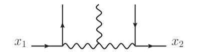
Figure 9: Potential contribution of one three-gluon vertex. Such terms are subleading due to the details of the momentum of vertices and propagators.

The other potential contributions arise from the gluon self-interactions; an example is shown in fig. (9). It is not difficult to see that, in a general renormalizable gauge, their momentum dependence leads, after Fourier transform, to factors of $|x_{12}|^{2}$ in the numerator which will soften the singularity in the null separation limit and render these diagrams subleading.

We can therefore conclude that

$$\lim_{x_{i,i+1}^{2}\to 0}\frac{\langle{\cal O}(x_{1})\dots\cal O(x_{n})\rangle}{\langle{\cal O}(x_{1})\dots\cal O(x_{n})\rangle_{0}}=\frac{\langle W_{n}\rangle_{\text{adj}}}{\langle W_{n}\rangle_{0,\text{adj}}}$$ (A.6)

for 2-field operators ${\cal O}$ constructed from scalars and fermions.

The arguments in § 4 carry over unmodified to the case when one or several additional operators are added to such correlation functions and kept at generic positions relative to the operators which become null-separated; we will not repeat them here. Similarly to the case of scalar operators, we find that the $n$-partial null limit, $|x_{i,i+1}|^{2}\rightarrow 0$ with $i=1,\dots,n$ and $n+1\equiv 1$, of the connected part of the correlation function of $n+m$ operators is given by

$$\lim_{x_{ii+1}^{2}\to 0}\frac{\langle{\cal O}(x_{1})\cdots{\cal O}(x_{n}){\cal O}(a_{1})\cdots{\cal O}(a_{m})\rangle^{\text{conn}}}{\langle{\cal O}(x_{1})\cdots{\cal O}(x_{n})\rangle}=\frac{\langle W_{n}\,{\cal O}(a_{1})\cdots{\cal O}(a_{m})\rangle^{\text{conn}}_{\text{adj}}}{\langle W_{n}\rangle_{\text{adj}}}\ .$$ (A.7)

A.2 Gauge fields

The Feynman diagrams contributing to correlation functions of two-field operators containing gauge field strengths do not follow the classification we have been using; this is because there are at least two operators between which there is no direct R-charge flow (i.e. if a flow exists at all it must pass through other operators). We will see, however, that unlike previous situation when absence of a flow led to absence of a sufficiently strong singularity in the null-separation limit, here a singularity does occur. The main difference compared to previous discussions relates to the existence of a derivative in the field strength acting along the sequence of propagators not carrying R-charge. As we will see, this will lead to the desired singularity in the limit in which a sequence of gluon propagators and three-point vertices stretch between two null-separated points.

Let us illustrate the mechanism at work by analyzing the simplest diagram – a single gluon propagator between two operators containing field strengths at points $x_{1}$ and $x_{2}$.

$$L(x_{1},x_{2})_{\mu\nu}^{\alpha\beta}=\left(-i\frac{\partial}{\partial x_{1}^{\mu}}\eta_{\nu\kappa}+i\frac{\partial}{\partial x_{1}^{\nu}}\eta_{\mu\kappa}\right)\eta^{\kappa\lambda}\left(-i\frac{\partial}{\partial x_{2}^{\alpha}}\eta_{\beta\lambda}+i\frac{\partial}{\partial x_{2}^{\beta}}\eta_{\alpha\lambda}\right)\int d^{d}p_{1}\frac{e^{ip_{1}\cdot(x_{1}-x_{2})}}{p_{1}^{2}+i0}.$$ (A.8)

The $p_{1}$ integral is exactly the same as that of a scalar propagator. Introducing a Schwinger-parameter and carrying out the momentum integral leads again to the position space scalar propagator, except that now there are two additional derivatives acting on it. Each derivative yields a factor of $\zeta^{-1}$, leading to

$$L(x_{1},x_{2}) = {}\frac{1}{4}\big{(}(x_{1}-x_{2})_{\mu}\eta_{\nu\kappa}-(x_{1}-x_{2})_{\nu}\eta_{\mu\kappa}\big{)}\eta^{\kappa\lambda}\big{(}(x_{2}-x_{1})_{\alpha}\eta_{\beta\lambda}-(x_{2}-x_{1})_{\beta}\eta_{\alpha\lambda}\big{)}$$ (A.9)

$$\times\int_{0}^{\infty}\frac{d\zeta}{\zeta^{2}}e^{-i\frac{(x_{1}-x_{2})^{2}}{4\zeta}-0/\zeta}\ .$$

This is again an integral of the type (18) and, following (19), it will be proportional to $(|x_{1}-x_{2}|^{2})^{-3+\epsilon}$. The singularity, stronger than that of a propagator between two scalar operators, is a reflection of the dimensional analysis.

It is not difficult to deduce the properties of a sequence of gluon propagators and three-gluon vertices. As in the case of scalar propagators, each gluon propagator brings one positive power of $\zeta$. To compensate for it and end up with a singularity as strong as (A.9) the null limit, each derivative in the 3-gluon vertex must yield a factor of $\zeta^{-1}$, in close analogy with the derivative in the scalar-gluon vertex – see § 3.1. Each such derivative also generates a factor of $(x_{1}-x_{2})^{\mu_{i}}$; due to the antisymmetry of the field strength contributions (cf. eq. (A.9)) these factors must carry the Lorentz indices of the out-going gluons. The details are essentially identical to those in sec. 3.1 and we will not repeat them here. The conclusion is that, up to a factor of $(|x_{1}-x_{2}|^{2})^{-3+\epsilon}$, the sequence of gluon propagators and three-point vertices between two null-separated points reduces in the null limit to a Wilson line with as many gluon vertices as the original number of vertices:

$$L(x_{1},x_{2},k)_{\mu\nu}^{\alpha\beta}{}_{\mu_{1}\dots\mu_{n}} \propto \big{(}(x_{1}-x_{2})_{\mu}\eta_{\nu\kappa}-(x_{1}-x_{2})_{\nu}\eta_{\mu\kappa}\big{)}\eta^{\kappa\lambda}\big{(}(x_{2}-x_{1})_{\alpha}\eta_{\beta\lambda}-(x_{2}-x_{1})_{\beta}\eta_{\alpha\lambda}\big{)}$$ (A.10)

$$\times\frac{1}{(|x_{1}-x_{2}|^{2})^{3-\epsilon}}\prod_{i=1}^{n}\;i(x_{1}-x_{2})_{\mu_{i}}\;\int_{t_{i-1}}^{1}dt_{i}\;e^{-i\sum_{i}k_{i}\cdot(x_{2}t_{i}-x_{1}(1-t_{i}))}\ ,$$

where the field strengths in the two operators at positions $x_{1}$ and $x_{2}$ carry indices $(\mu,\nu)$ and $(\alpha,\beta)$, respectively.

Other diagrams, in which the sequence of gluons is interrupted by scalars, fermions or ghosts will have subleading contributions in the null limit. Similarly, four-point Lagrangian vertices as well as the commutator terms in the field strength will drop out for the same reason.

Thus, similarly to the correlation function of operators constructed out of scalars and fermions, correlation functions of operators containing field strengths reduce to the expectation value of a null polygonal Wilson loop with cusps at the positions of the original operators. As in the case of correlation functions of operators without gauge fields, inclusion of one or more operators at generic positions relative to the null separation points is straightforward with the same result quoted in eqs. (6) and (7).

References

- [1] L. F. Alday, J. M. Maldacena, “Gluon scattering amplitudes at strong coupling,” JHEP 0706, 064 (2007). [arXiv:0705.0303 [hep-th]].
- [2] G. P. Korchemsky, J. M. Drummond, E. Sokatchev, “Conformal properties of four-gluon planar amplitudes and Wilson loops,” Nucl. Phys. B795, 385-408 (2008). [arXiv:0707.0243 [hep-th]]. A. Brandhuber, P. Heslop, G. Travaglini, “MHV amplitudes in N=4 super Yang-Mills and Wilson loops,” Nucl. Phys. B794, 231-243 (2008). [arXiv:0707.1153 [hep-th]].
- [3] E. I. Buchbinder, A. A. Tseytlin, “On semiclassical approximation for correlators of closed string vertex operators in AdS/CFT,” JHEP 1008, 057 (2010). [arXiv:1005.4516 [hep-th]]. R. A. Janik, P. Surowka, A. Wereszczynski, “On correlation functions of operators dual to classical spinning string states,” JHEP 1005, 030 (2010). [arXiv:1002.4613 [hep-th]].
- [4] L. F. Alday, B. Eden, G. P. Korchemsky, J. Maldacena, E. Sokatchev, “From correlation functions to Wilson loops,” [arXiv:1007.3243 [hep-th]].
- [5] B. Eden, P. Heslop, G. P. Korchemsky, E. Sokatchev, “The super-correlator/super-amplitude duality: Part I,” [arXiv:1103.3714 [hep-th]].
- [6] B. Eden, P. Heslop, G. P. Korchemsky, E. Sokatchev, “The super-correlator/super-amplitude duality: Part II,” [arXiv:1103.4353 [hep-th]].
- [7] T. Adamo, M. Bullimore, L. Mason, D. Skinner, “A Proof of the Supersymmetric Correlation Function / Wilson Loop Correspondence,” [arXiv:1103.4119 [hep-th]].
- [8] M. Bullimore, D. Skinner, “Holomorphic Linking, Loop Equations and Scattering Amplitudes in Twistor Space,” [arXiv:1101.1329 [hep-th]].
- [9] B. Eden, G. P. Korchemsky, E. Sokatchev, “From correlation functions to scattering amplitudes,” [arXiv:1007.3246 [hep-th]].
- [10] D. E. Berenstein, R. Corrado, W. Fischler and J. M. Maldacena, “The operator product expansion for Wilson loops and surfaces in the large N limit,” Phys. Rev. D 59, 105023 (1999) [arXiv:hep-th/9809188].
- [11] K. Zarembo, “Open string fluctuations in and operators with large R charge,” Phys. Rev. D 66, 105021 (2002) [arXiv:hep-th/0209095].
- [12] V. Pestun and K. Zarembo, “Comparing strings in to planar diagrams: An Example,” Phys. Rev. D 67, 086007 (2003) [arXiv:hep-th/0212296].
- [13] J. Gomis, S. Matsuura, T. Okuda and D. Trancanelli, “Wilson loop correlators at strong coupling: from matrices to bubbling geometries,” JHEP 0808, 068 (2008) [arXiv:0807.3330].
- [14] L. F. Alday and A. A. Tseytlin, “On strong-coupling correlation functions of circular Wilson loops and local operators,” arXiv:1105.1537 .
- [15] A. Miwa and T. Yoneya, “Holography of Wilson-loop expectation values with local operator insertions,” JHEP 0612, 060 (2006) [hep-th/0609007]. M. Sakaguchi and K. Yoshida, “A Semiclassical String Description of Wilson Loop with Local Operators,” Nucl. Phys. B 798, 72 (2008) [arXiv:0709.4187]. A. Miwa, “BMN operators from Wilson loop,” JHEP 0506, 050 (2005). [hep-th/0504039]. G. W. Semenoff, D. Young, “Exact 1/4 BPS Loop: Chiral primary correlator,” Phys. Lett. B643, 195-204 (2006). [hep-th/0609158].
- [16] L. F. Alday, E. I. Buchbinder, A. A. Tseytlin, “Correlation function of null polygonal Wilson loops with local operators,” [arXiv:1107.5702 [hep-th]].
- [17] B. Eden, C. Schubert, E. Sokatchev, “Three loop four point correlator in N=4 SYM,” Phys. Lett. B482, 309-314 (2000). [hep-th/0003096].
- [18] L. F. Alday, J. Maldacena, “Comments on gluon scattering amplitudes via AdS/CFT,” JHEP 0711, 068 (2007). [arXiv:0710.1060 [hep-th]].
- [19] J. Maldacena, A. Zhiboedov, “Form factors at strong coupling via a Y-system,” JHEP 1011, 104 (2010). [arXiv:1009.1139 [hep-th]].
- [20] B. Eden, P. Heslop, G. P. Korchemsky, E. Sokatchev, “Hidden symmetry of four-point correlation functions and amplitudes in N=4 SYM,” [arXiv:1108.3557 [hep-th]].
- [21] A. V. Belitsky, A. S. Gorsky, G. P. Korchemsky, “Gauge / string duality for QCD conformal operators,” Nucl. Phys. B667, 3-54 (2003). [arXiv:hep-th/0304028 [hep-th]].
- [22] E. I. Buchbinder, A. A. Tseytlin, “Semiclassical four-point functions in ,” JHEP 1102, 072 (2011). [arXiv:1012.3740 [hep-th]].
- [23] R. Roiban, A. A. Tseytlin, “On semiclassical computation of 3-point functions of closed string vertex operators in ,” Phys. Rev. D82, 106011 (2010). [arXiv:1008.4921 [hep-th]].
- [24] M. S. Costa, R. Monteiro, J. E. Santos, D. Zoakos, “On three-point correlation functions in the gauge/gravity duality,” JHEP 1011, 141 (2010). [arXiv:1008.1070 [hep-th]].
- [25] R. Roiban and A. A. Tseytlin, “Quantum Strings in S5: Strong-Coupling Corrections to Dimension of Konishi Operator,” JHEP 0911 (2009) 013 [arXiv:0906.4294 [hep-th]].
- [26] A. Tirziu and A. A. Tseytlin, “Quantum Corrections to Energy of Short Spinning String in AdS5,” Phys. Rev. D 78 (2008) 066002 [arXiv:0806.4758 [hep-th]].
- [27] M. Bullimore, D. Skinner, “Holomorphic Linking, Loop Equations and Scattering Amplitudes in Twistor Space,” [arXiv:1101.1329 [hep-th]].
- [28] N. Arkani-Hamed, J. L. Bourjaily, F. Cachazo, S. Caron-Huot, J. Trnka, “The All-Loop Integrand For Scattering Amplitudes in Planar N=4 SYM,” JHEP 1101, 041 (2011). [arXiv:1008.2958 [hep-th]].
- [29] R. H. Boels, “On BCFW shifts of integrands and integrals,” JHEP 1011, 113 (2010). [arXiv:1008.3101 [hep-th]].
- [30] S. Raju, “Recursion Relations for AdS/CFT Correlators,” Phys. Rev. D83, 126002 (2011). [arXiv:1102.4724 [hep-th]].
- [31] R. Boels, K. J. Larsen, N. A. Obers, M. Vonk, “MHV, CSW and BCFW: Field theory structures in string theory amplitudes,” JHEP 0811, 015 (2008). [arXiv:0808.2598 [hep-th]].
- [32] C. Cheung, D. O’Connell, B. Wecht, “BCFW Recursion Relations and String Theory,” JHEP 1009, 052 (2010). [arXiv:1002.4674 [hep-th]].
- [33] R. H. Boels, D. Marmiroli and N. A. Obers, “On-Shell Recursion in String Theory,” JHEP 1010 (2010) 034 [arXiv:1002.5029 [hep-th]].