Bound states in open coupled asymmetrical waveguides and quantum wires

Abstract

The behavior of bound states in asymmetric cross, T and L shaped configurations is considered. Because of the symmetries of the wavefunctions, the analysis can be reduced to the case of an electron localized at the intersection of two orthogonal crossed wires of different width. Numerical calculations show that the fundamental mode of this system remains bound for the widths that we have been able to study directly; moreover, the extrapolation of the results obtained for finite widths suggests that this state remains bound even when the width of one arm becomes infinitesimal. We provide a qualitative argument which explains this behavior and that can be generalized to the lowest energy states in each symmetry class. In the case of odd-odd states of the cross we find that the lowest mode is bounded when the width of the two arms is the same and stays bound up to a critical value of the ratio between the widths; in the case of the even-odd states we find that the lowest mode is unbound up to a critical value of the ratio between the widths. Our qualitative arguments suggest that the bound state survives as the width of the vertical arm becomes infinitesimal.

I INTRODUCTION

Trapped waves in open geometries have been known for sixty years now Ursell:1951 . Ursell Ursell:1952 , in a theoretical and experimental study of “beach” waves in a particular semi–infinite canal, found that the system has discrete, continuous and mixed spectra, and predicted the existence of a confined resonance at a discrete frequency, while at a cutoff frequency the resonance extends a long way down the canal. These waves can be described by the Helmholtz equation subject to Dirichlet boundary conditions and therefore similar confinement properties are expected in the solutions of analogous acoustic or electromagnetic problems. Indeed, about fifteen years after Ursell, long-lived resonance modes in open laser systems were reportedWeinstein:1966 . Even more, since this setup is equivalent to that of electrons in open configurations described by the time-independent Schrödinger equation, by 1984, several studies already suggested that confinement is also a feature of the two-dimensional transport of charge carriers in ultrafine metal and semiconductor devicesSakaki:1984 . From then on, many theoretical and experimental studies have shown that, generally, by bending and crossing waveguides and quantum wires, bound (confined, trapped) states can be obtained with energies below the continuous spectrumCarini:1997 . Moreover, many similar quantum wire systems have been found with bound states embedded into the continuumLondergan:1999 .

Bound states just below the continuum may strongly influence the scattering of waves and charge carriers. This allows to detect them and it is also the source of new phenomena and applications. For instance, mesoscopic systems with similar geometries are common in nanoelectronics and it has been shown experimentally that they exhibit suppression (“quenching”) of the Hall resistanceRoukes:1988 , and enhanced bend resistanceTimp:1988 . On the other hand, if the above mentioned bound states exist only due to a particular symmetry, when this symmetry is broken, resonances could be expected to arise. Therefore, the confinement of electromagnetic radiation at the intersection of coupled waveguides opens a window for a new kind of resonator, which combines a very simplified spectrum to high performancesAnnino:2006 . Similar phenomena should be also relevant for the performance of novel kinds of (cold) atomBromley:2003 , phononQu:2004 and laser waveguidesHill:2007 . Even more, the possibility of geometrically inducing confined states allows for the design of unused ways to create a Bose-Einstein condensate in a quasi-one dimensional Bose gasExner:2005 . Last but not least, besides the possible practical applications, it should be noted that such systems constitute a very interesting theoretical framework for studying the correspondence between classical and quantum dynamics. Note that, in this kind of arrangements, classical motion of point particles with finite energy is typically unbound because there are not forbidden regions along the wires. Therefore, a phase-space semiclassical approximation to dynamics seems to be not valid here, and this is particularly relevant if the corresponding classical motion exhibits chaosExner:1996 .

A relevant question, from both the theoretical and experimental point of view, is how strongly depend the properties of the bound states on the perturbation of the structure and, this way, on the mechanical imperfections. Amongst other factors, is perhaps the symmetry of the configuration what plays the fundamental role since it controls the coupling with the propagating modes. Some studies suggested that the isolated bounded modes are not affected by the level of symmetry and thus, they can exist under very general conditionsAnnino:2006b . Nevertheless, a comprehensive analysis of the role of symmetry is still lacking.

In a classical paper written more than twenty years ago Schult, Ravenhall and WyldSchult89 studied the problem of an electron which can freely move in a two dimensional symmetric region of orthogonally crossed wires of finite width and infinite length. They showed that the ground state of this system corresponds to a state where the electron is confined in the region of the crossing, with an energy which falls below the threshold of the continuum, $E_{\rm TH}$. Using two different numerical approaches (finite differences and a mode expansion) they estimated the ratio between the ground state energy and the threshold energy, $E_{1}/E_{\rm TH}\approx 0.66$. They also identified a second bound state, with odd-odd symmetry, corresponding to a ratio $E_{2}/E_{ŧh}\approx 3.72$. The energy of this second state falls below the threshold of the continuum for odd-odd states. These results were later confirmed by Avishai et al.Avishai91 . More recently, Amore, Fernández and RodriguezAmore11 , have used the Conformal Collocation method (CCM)Amore08 to obtain a precise value for the ground state of the infinite cross, using a non uniform grid. They obtained $E_{1}/E_{\rm TH}\approx 0.659611$. Trefethen and BetckeTrefethen06 , on the other hand have obtained a precise value for the second bound state, $E_{2}/E_{\rm TH}\approx 3.71648$ (notice that these authors report the value of $E_{2}$, from which the ratio can be obtained).

Different geometries are closely related to the symmetric cross. Bulgakov and collaborators have studied the properties of a configuration of non-orthogonal (“scissor-shaped”) crossed wires, observing the emergence of multiple bound states below the continuum as the angle between the arms is reduced Bulgakov02 . A particular case of T-shaped waveguide is obtained from the symmetric cross by desymmetrizing the region for even-odd modes, although this particular system does not support bound states. Nazarov Nazarov10 , analyzed the bound states of a similar configuration, but with arms of different widths.

Taking into account the above mentioned relevance of the symmetries for the spectrum, in this paper we study a different modification of the case discussed by Schult et al.Schult89 , considering an asymmetric cross, with orthogonal arms of different width. Our goal is to investigate the behavior of the bound states of this system, as one of the arms is enlarged, and the possibility of the disappearance of these states or the appearance of new bound states. The related L and T shaped configurations are also analyzed.

The paper is organized as follows: in Section II we describe the system of the asymmetric cross and we make qualitative predictions on the behavior of the bound states as one of the arms is enlarged; in Section III we present the numerical results, which have been obtained using a collocation method; finally, in Section IV we draw our conclusions.

II The asymmetric cross

As we have mentioned in the Introduction, Schult, Ravenhall and WyldSchult89 have proved that an electron which moves freely in an infinite symmetric cross is localized in the central region of the cross when it finds itself in the ground state. They also discovered a second localized state, which is the lowest energy state with odd-odd symmetry.

The goal of our paper is to investigate the behavior of these modes (as well as the possible appearance of further localized states), as the width of one of the two arms is changed, thus obtaining the asymmetric cross, shown in Fig. 1.

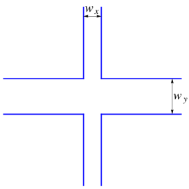
Figure 1: (color online) Asymmetric cross

In particular, we ask ourselves whether the localized modes of the symmetric cross can survive to arbitrary perturbations of this kind: what happens when one of the arms is much smaller than the other? Would we still have bound states? What does this imply for the L and T shaped configurations?

To answer our questions we need to solve the scalar Helmholtz equation

$$-\frac{1}{2}\ \Delta\Psi_{n}(x,y)=E_{n}\Psi_{n}(x,y)\ ,$$ (1)

where $(x,y)\in\Omega=\left\{|x|<w_{x}/2,|y|<w_{y}/2\right\}$ and we are using $\hbar/m=1$. The wave functions obey Dirichlet boundary conditions on $\partial\Omega$. We have called $w_{x}$ and $w_{y}$ the widths of the two arms, defining $\beta\equiv w_{y}/w_{x}$ (for $\beta=1$ one recovers the symmetric cross).

Before trying to answer our question in a quantitative way, we may attack the problem qualitatively. Let us consider the case $\beta\gg 1$, meaning that the width of the horizontal arm is much larger than the width of the vertical arm, and assume that there is at least one localized solution to eq.(1). This situation is represented in fig.2:

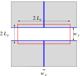
Figure 2: (color online) Highly asymmetric cross: $w_{x}\ll w_{y}$.

the grey regions in this plot represent the forbidden region, where the eigenfunctions of eq. (1) must vanish identically; we assume that the dimensions of the red rectangle are large enough so that the localized wave functions are exponentially small outside the rectangle.

Under these assumptions, one may attempt an approximate solution of the original problem inside the rectangle, and thus obtain accurate approximations to the bound states of eq. (1), if they exist.

The fundamental idea is to represent eq. (1) as a Schrödinger equation

$$\left[-\frac{1}{2}\Delta+V(x,y)\right]\Psi_{n}(x,y)=E_{n}\Psi_{n}(x,y)\ ,$$ (2)

with

$$V(x,y) = \left\{\begin{array}[]{ccc}0&,&(x,y)\in\Omega\\ \infty&,&(x,y)\not\in\Omega\end{array}\right.\ .$$ (5)

To allow numerical calculation the exact potential $V(x,y)$ is replaced by an approximate potential $\tilde{V}(x,y)$:

$$\tilde{V}(x,y) = \left\{\begin{array}[]{ccc}0&,&(x,y)\in\Omega\\ V_{0}&,&(x,y)\not\in\Omega\end{array}\right.\ ,$$ (8)

which takes a large but finite value $V_{0}$ in the forbidden region. If $V_{0}$ is large enough (much larger than the energies of the lowest states), the wave functions of these states are exponentially suppressed in the classically forbidden region (the grey region in the figure), and the contribution from this region becomes negligible.

The advantage of reformulating the problem in this way should be clear, since we may now work on the entire rectangle, $(x,y)\in\mathcal{D}=\left\{|x|\leq L_{x},|y|\leq L_{y}\right\}$, and use the orthonormal basis

$$\Phi_{n_{x},n_{y}}(x,y) = \chi_{n_{x}}(x)\ \zeta_{n_{y}}(y)\ ,$$

with

$$\chi_{n_{x}}(x) = \sqrt{\frac{1}{L_{x}}}\ \sin\frac{n_{x}\pi(x+L_{x})}{2L_{x}}\ ,$$

$$\zeta_{n_{y}}(x) = \sqrt{\frac{1}{L_{y}}}\ \sin\frac{n_{y}\pi(y+L_{y})}{2L_{y}}\ .$$

and $n_{x},n_{y}=1,2,\dots$.

Kaufman, Kosztin and Schulten Kaufman99 have used this approach to calculate approximations to the eigenvalues and eigenfunctions of the negative Laplacian on finite domains, applying the Rayleigh-Ritz method to the Schrödinger equation with $V(x,y)\rightarrow\tilde{V}(x,y)$ on a rectangular domain fully enclosing the region.

The accuracy of this method clearly depends both on the finite value of the potential step $V_{0}$ used in the numerical calculation and the ratio between the areas of $\mathcal{D}$ and the portion of area of $\Omega$ falling inside $\mathcal{D}$ (which we call $\tilde{\Omega}$): if the area of $\mathcal{D}$ is much larger than the area of $\tilde{\Omega}$, a large number of basis functions will be needed in the calculation to achieve a suppression of the wavefunctions in the classically forbidden regions.

Since we are interested in the limit $L_{x}\gg L_{y}$, we may use a simpler and more direct approach: provided that the rectangle $\mathcal{D}$ is very thin, the lowest modes of eq.(2) on $\mathcal{D}$ will be dominated by the longitudinal modes of the basis, with negligible contributions from the transverse excited modes.

This observation justifies the possibility of using a portion of the Hilbert space of the problem, corresponding to the states $\Phi_{n_{x},1}(x,y)$.

In this limit the “high–energy” modes essentially decouple from the problem and we may work with an effective Hamiltonian, obtained by averaging the original Hamiltonian with respect to the mode $\zeta_{1}(y)$:

$$\hat{H}_{eff}(x) \equiv \int_{-L_{y}}^{L_{y}}dy\ \zeta_{1}(y)\hat{H}\ \zeta_{1}(y)$$

$$= -\frac{1}{2}\frac{\partial^{2}}{\partial x^{2}}+\frac{\pi^{2}}{8L_{y}^{2}}+V_{eff}(x)\ ,$$

where the effective potential is

$$V_{eff}(x) \equiv \int_{-L_{y}}^{L_{y}}dy\ \zeta_{1}^{2}(y)\tilde{V}(x,y)$$ (11)

$$= \left\{\begin{array}[]{ccc}0&,&|x|\leq w_{x}/2\\ 2V_{0}\int_{w_{y}/2}^{L_{y}}\zeta_{1}(y)^{2}dy&,&|x|>w_{x}/2\\ \end{array}\right.$$

With this qualitative argument we find that the effective potential behaves as a square well of finite depth (which we will denote by $\Delta$), whose width is precisely the width of the smaller arm, $w_{x}$ (see the left plot of fig.3).

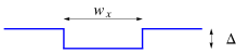
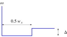
Figure 3: (color online) Effective potentials corresponding to figs. 2 and 5 (left) and to figs.4 and 6 (right)

It is well known that the ground state of this potential is always bound, independently of the width and depth of the well. On these grounds we expect that the fundamental mode of the asymmetric cross of fig.2 will always be bound, regardless of the width of the two arms, as long as they are finite!

We can also study the remaining lowest modes in each symmetry class using the same approach. In Figs.4, 5 and 6 we display the desymmetrized regions corresponding to the symmetry classes of modes with odd-even, even-odd and odd-odd respectively. Repeating the same steps followed for the full domain of fig.2, we may easily convince ourselves that the effective potential of Figs.4 and 6 corresponds to a finite well potential with a infinite wall on one side (see the left plot of fig.3), whereas the case of Fig.5 is analogous to the one of Fig.2.

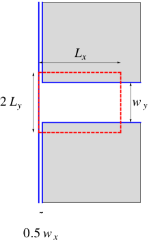
Figure 4: (color online) T-shaped configuration; desymmetrized region for odd-even modes of the asymmetric cross.

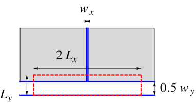
Figure 5: (color online) T-shaped configuration; desymmetrized region for even-odd modes of the asymmetric cross.

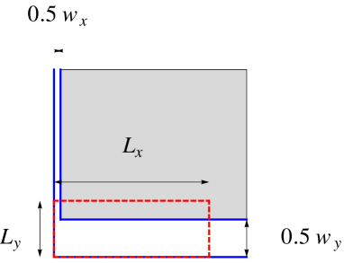
Figure 6: (color online) L-shaped configuration; desymmetrized region for odd-odd modes of the asymmetric cross.

The simple quantum mechanical problem for the potential well of the right plot of fig.3 does not admit localized solutions when the potential well is either very narrow or very shallow.

These simple arguments allow us to make the following predictions:

• the fundamental mode of the symmetric cross stays always bounded, as the width of one of the two arms is increased arbitrarily, but remains finite;

• the fundamental mode of a domain with the shape of an infinite L (which is the lowest energy odd-odd mode of the symmetric cross) is bounded, but becomes unbounded as the width of any of the two arms is increased, while keeping fixed the width of the other arm;

• the fundamental mode of an infinite T shaped domain (even-odd modes of the asymmetric cross), shown in Fig.5, is not bound for the symmetric cross, but it becomes bound as the width $w_{x}\rightarrow 0$, but remains finite;

• the fundamental mode of the “rotated” T of fig. 4 (odd-even modes of the asymmetric cross), is not bound either for the symmetric cross or as $w_{x}\rightarrow 0$.

Notice that the predictions regarding the T-shaped infinite domain in Fig.5 are in agreement with the findings of Nazarov Nazarov10 .

In the next Section we describe the numerical methods that we have used to test these predictions and we present the numerical results obtained with these methods.

III Numerical results

The correctness of the analysis in the previous section strongly depends on the assumption of the decoupling of the “high-energy” modes which leads to an effective one-dimensional problem. However, we are interested in any perturbation of the symmetry, not only the large ones given by $\beta\gg 1$. Thus, here we verify, by numerically solving eq. (1), that the results obtained in the previous section are correct, and, even more, that our predictions can be extrapolated to the whole range of possible values of $\beta$.

We now illustrate the method that we have used in our calculations. Upon a simple rescaling of the $y$ axis, defining $y^{\prime}=y/\beta$ ($x^{\prime}=x$), we write eq.(1) in the form of a modified Helmholtz equation

$$-\left(\frac{\partial^{2}}{\partial{x^{\prime}}^{2}}+\frac{1}{\beta^{2}}\frac{\partial^{2}}{\partial{y^{\prime}}^{2}}\right)\psi_{n}(x^{\prime},y^{\prime})=E_{n}\psi_{n}(x^{\prime},y^{\prime})\ ,$$ (12)

which allows us to work on an infinite symmetric cross of width $w_{x}$, with $\beta$ playing a role of a parameter.

As we are interested in the bound states of eq. (12), we may “cut” the cross at some large but finite distances $L_{x}$ and $L_{y}$, by imposing Dirichlet boundary conditions at $x=\pm L_{x}$ and $y=\pm L_{y}$. If $L_{x}$ and $L_{y}$ are large enough the wave functions of the bound states are exponentially small at larger distances and the error introduced by this approximation is negligible compared to the error due to the discretization. In general, for $\beta\gg 1$, one may choose $L_{x}\gg L_{y}$, as the probability density is mostly concentrated on the wider arm. The maximum size of $L_{x}$ and $L_{y}$ is essentially dictated by the total number of collocation points corresponding to this choice.

On the other hand, excessively large values of $L_{x}$ and $L_{y}$ should be avoided, since they increase the number of collocation points and therefore the computational power needed in the calculation.

To discretize eq. (12) we use a collocation approach based on “tent functions” (TF): on the interval $|x|\leq L$ we define the uniform grid, whose $N-1$ points are $x_{k}\equiv{2Lk}/{N}$, where $N$ is an even integer and $k=-N/2+1,-N/2+2,\dots,N/2-1$. The tent function peaked at the point $x_{k}$ is defined as:

$$\phi_{k}(x) \equiv \left\{\begin{array}[]{ccc}\frac{x-x_{k-1}}{x_{k}-x_{k-1}}&,&x_{k-1}\leq x\leq x_{k}\\ \frac{x_{k+1}-x}{x_{k+1}-x_{k}}&,&x_{k}\leq x\leq x_{k+1}\\ 0&,&x<x_{k-1},x>x_{k+1}\\ \end{array}\right.$$ (16)

A function $f(x)$ obeying Dirichlet boundary conditions at $x=\pm L$ ($f(\pm L)=0$) can be interpolated using the TF as

$$f^{(TF)}(x)=\sum_{k=-N/2+1}^{N/2-1}f(x_{k})\phi_{k}(x)\approx f(x)\ .$$

For a higher dimensional problem, the same procedure may be followed, using multidimensional TFs which are the direct product of the TFs along each orthogonal direction:

$$\Phi_{k_{1},k_{2},\dots,k_{d}}(x_{1},x_{2},\dots,x_{d}) = \phi_{k_{1}}(x_{1})\ \phi_{k_{2}}(x_{2})\ \dots\ \phi_{k_{d}}(x_{d})$$

In principle the interpolation of a d-dimensional function on a d-dimensional region $|x_{i}|\leq L_{i}$, requires $M=\prod_{i=1}^{d}(N_{i}-1)$ points.

The eigenvalue equation (12) may then be converted to a matrix eigenvalue problem calculating the matrix elements of the Hamiltonian operator between all the functions of a set: the size of the matrix depends on the total number of functions used in the calculation, which rapidly grows with the dimensionality of the problem. A drastic reduction of the number of functions however can be achieved by considering only functions which are peaked at points internal to the cross.

A second observation concerns the choice of $N_{i}$, i.e. the number of collocation points in each orthogonal direction: although in principle, $N_{i}$ ($i=1,\dots d$) can take any integer value, it is convenient to pick values of $N_{i}$ which allow to sample exactly the border of the cross. The eigenvalues obtained for different grids sampling the border of the domain provide a monotonous sequence of values, which allows to obtain a good approximation via extrapolationAmore10e .

Before calculating the eigenvalues of the asymmetric cross, we have tested this collocation method on the symmetric cross, for which a precise result is available Amore11 . The method used in that case is the conformal collocation method (CCM) Amore08 . Working with grids with $N=N_{x}=N_{y}=80,120,\dots,880$ we have calculated the lowest eigenvalue of the corresponding collocation matrix, obtaining a monotonous sequence of values: the most accurate value, corresponding to the finest grid, provides a ratio $E_{1}/E_{\rm TH}=0.66166$, which is just $0.3\%$ above the value reported by Amore et al. Amore11 We have also performed a least square fit of the monotonous sequence of values with the functional form $a_{1}+a_{2}/N^{\gamma}+a_{3}/N^{2\gamma}+a_{4}/N^{3\gamma}$, obtaining $a_{1}=0.65955$, which differs just for the $0.1\%$ from the value previously reportedAmore11 . This test makes us confident that our results are precise.

We can now present the results obtained for the asymmetric cross, discussing separately the states with different symmetries. In all cases we expect that the wave function of a bound state will decay exponentially as one moves far away from the center of the cross; in particular, the effective Hamiltonian approach that we have described in the previous section predicts $\Psi(x,y)|_{y\rm\ fixed}\approx e^{-x/\ell_{x}}$ for $|x|\gg w_{x}/2$, in the limit $\beta\gg 1$. We have found that there is at most only one bound state in each symmetry class.

III.1 Even-even state

We first study the lowest energy state with even-even symmetry of the asymmetric cross. In the third column of Table 1

Table 1: The ratio $E^{\rm(ee)}/E_{\rm TH}$ for the lowest even-even state of the asymmetric cross. Set I corresponds to using $L=20$ and $N=600$; Set II corresponds to using $L=40$ and $N=800$; Set III corresponds to using $L=100$ and $N=1600$.

$\beta$	Set	$E^{\rm(ee)}/E_{\rm TH}$	$\ell_{x}$	$\ell_{y}$
1.0	I	0.662960	1.098	1.098
1.1	I	0.723925	1.335	1.006
1.2	I	0.774665	1.613	0.938
1.3	I	0.816242	1.936	0.887
1.4	I	0.849968	2.309	0.847
1.5	II	0.879058	2.770	0.818
1.6	II	0.900702	3.267	0.793
1.7	II	0.918059	3.830	0.773
1.8	II	0.931999	4.463	0.757
1.9	II	0.943228	5.172	0.744
2.0	II	0.952308	5.960	0.733
2.1	II	0.959682	6.832	0.723
2.2	III	0.965821	7.959	0.717
2.3	III	0.970627	9.053	0.711
2.4	III	0.974578	10.252	0.705
2.5	III	0.977844	11.564	0.700
2.6	III	0.980557	12.992	0.696
2.7	III	0.982821	14.542	0.695
2.8	III	0.984719	16.219	0.690
2.9	III	0.986319	18.026	0.689
3.0	III	0.987674	19.965	0.685

we report the values of the ratio $E^{\rm(ee)}/E_{\rm TH}$, obtained for different values $\beta$. We used three different sets, corresponding to $L=20$ and $N=600$ (set I), $L=40$ and $N=800$ (set II) and $L=100$ and $N=1600$ (set III). The fourth and fifth column report the values of the decay lengths $\ell_{x}$ and $\ell_{y}$ obtained fitting the numerical eigenfunctions with the asymptotic behaviors $\Psi(x,0)\approx e^{-x/\ell_{x}}$ and $\Psi(0,y)\approx e^{-y/\ell_{y}}$, respectively for $|x|\gg w_{x}/2$ and $|y|\gg w_{y}/2$.

These values are plotted in Figs.7 and 8.

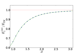
Figure 7: (color online) Ratio $E^{(\rm ee)}/E_{\rm TH}$ as a function of $\beta$ for the asymmetric cross; the solid line is the least squares fit $\left.E_{1}/E_{\rm TH}\right|^{\rm FIT}=1.003-{0.505}{\beta^{-3.23725}}+{0.165}{\beta^{-6.475}}$.

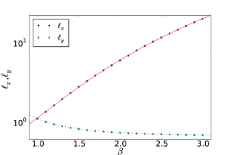
Figure 8: (color online) $\ell_{x}$ and $\ell_{y}$ as a function of $\beta$ for the lowest even-even state of the asymmetric cross; the solid and dashed lines are the least squares fits $\left.\ell_{x}\right|^{\rm FIT}=0.472+0.644\ \beta^{3.104}$ and $\left.\ell_{y}\right|^{\rm FIT}=0.656+{0.443}{\beta^{-2.503}}$.

The dependence on $\beta$ is described very accurately by simple least square fits. In particular, within the accuracy of our calculations, the fit of $E^{\rm(ee)}/E_{\rm TH}$ is consistent with the survival of the bound state for $\beta\rightarrow\infty$.

Notice that $\ell_{x}$ grows roughly cubically in $\beta$ for $\beta\gg 1$, limiting the range of values of $\beta$ where the numerical calculation can be performed. As an example, in figs.9 and 10 we show different representations of our numerical results for the wave function of the lowest even-even state for $\beta=2$ (in these figures, as well in the other figures representing the wavefunctions, the region of the plot is smaller than the actual region where the numerical calculations were performed).

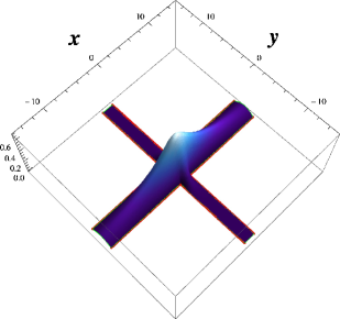
Figure 9: (color online) Wave function of the lowest even-even state for $\beta=2$.

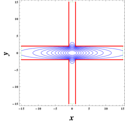
Figure 10: (color online) Wave function of the lowest even-even state for $\beta=2$.

III.2 Odd-odd state

As it was found by Schult, Ravenhall and WyldSchult89 the symmetric cross ($\beta=1$) has a second bound state, which has odd-odd symmetry and therefore it is also an eigenstate of an infinite L. According to our qualitative discussion based on an effective Hamiltonian, we expect that this state may become unbound at some finite $\beta$.

In Table 2 we report the results for the ratio $E^{\rm(oo)}/E_{\rm TH}$ (second column) and for the longitudinal and transverse length scales, $\ell_{x}$ and $\ell_{y}$ (third and fourth columns). In this case the length scales are obtained fitting the asymptotic behavior of the wave function with $\Psi(x,w_{y}/3)\approx e^{-x/\ell_{x}}$ and $\Psi(w_{y}/3,y)\approx e^{-y/\ell_{y}}$, respectively for $|x|\gg w_{x}/2$ and $|y|\gg w_{y}/2$, since the wave function vanishes for $x=0$ or $y=0$.

Table 2: The ratio $E^{\rm(oo)}/E_{\rm TH}$ for the lowest odd-odd state of the asymmetric cross. All the results are obtained using $L=100$ and $N=1600$.

$\beta$	$E^{\rm(oo)}/E_{\rm TH}$	$\ell_{x}$	$\ell_{y}$
1.00	3.72042	1.332	1.332
1.01	3.75611	1.465	1.232
1.02	3.78877	1.623	1.148
1.03	3.81839	1.816	1.076
1.04	3.84499	2.055	1.014
1.05	3.86855	2.359	0.960
1.06	3.88909	2.760	0.912
1.07	3.90659	3.313	0.870
1.08	3.92107	4.125	0.832
1.09	3.93252	5.429	0.797
1.10	3.94095	7.875	0.766
1.11	3.94635	14.119	0.739
1.111	3.94673	15.322	0.735
1.112	3.94707	16.745	0.733
1.113	3.94739	18.456	0.730
1.114	3.94767	20.549	0.728
1.115	3.94792	23.167	0.726
1.116	3.94815	26.528	0.722

In Fig.11

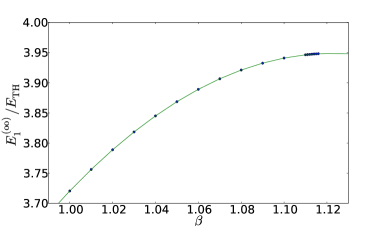
Figure 11: (color online) Ratio $E^{(\rm oo)}/E_{\rm TH}$ as a function of $\beta$ for the asymmetric cross; the solid line is the least squares fit $\left.E_{1}^{({\rm oo})}/E_{\rm TH}\right|^{\rm FIT}=-15.61-15.56\beta^{1.974}+34.88\beta^{0.9869}$.

we report the results for $E^{(\rm oo)}/E_{\rm TH}$ of the Table 2 and compare them with the least squares fit

$$\left.E_{1}^{({\rm oo})}/E_{\rm TH}\right|^{\rm FIT}=-15.61-15.56\beta^{1.974}+34.88\beta^{0.9869}\,.$$

Notice that the fit has a maximum corresponding to $\beta=1.12288$.

In Fig.12

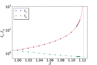
Figure 12: (color online) $\ell_{x}$ and $\ell_{y}$ as a function of $\beta$ for the lowest odd-odd state of the asymmetric cross; the solid and dashed lines are the least squares fits $\left.\ell_{x}\right|^{\rm FIT}={0.0108614}/({1-0.992232\beta^{0.0673327}})$ and $\left.\ell_{y}\right|^{\rm FIT}=0.514767+{0.81312}{\beta^{-12.3632}}$. The vertical line corresponds to the critical value $\beta^{({\rm oo})}_{\star}=1.2279$ where $\left.\ell_{x}\right|^{\rm FIT}$ is singular.

we display the length scales $\ell_{x}$ and $\ell_{y}$ as functions of $\beta$, and compare them with the fits

$$\left.\ell_{x}\right|^{\rm FIT}=\frac{0.0108614}{1-0.992232\beta^{0.0673327}}$$

and

$$\left.\ell_{y}\right|^{\rm FIT}=0.514767+\frac{0.81312}{\beta^{12.3632}}.$$

We believe that this plot offers convincing evidence of the existence of a singularity in $\ell_{x}$ close to $\beta^{({\rm oo})}_{\star}=1.2279$: for $\beta\geq\beta^{({\rm oo})}_{\star}$ the wave function becomes unbound, in agreement with our earlier prediction. As an example, in figs.13 and 14 we show different representations of our numerical results for the wave function of the lowest odd-odd state for $\beta=1.1$.

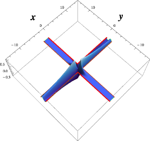
Figure 13: (color online) Wave function of the lowest odd-odd state for $\beta=1.1$.

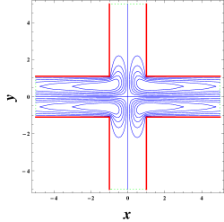
Figure 14: (color online) Wave function of the lowest odd-odd state for $\beta=1.1$.

III.3 Even-odd state

In Table 3

Table 3: The ratio $E^{\rm(eo)}/E_{\rm TH}$ for the lowest odd-odd state of the asymmetric cross. All the results are obtained using $L=100$ and $N=1600$.

$\beta$	$E^{\rm(eo)}/E_{\rm TH}$	$\ell_{x}$	$\ell_{y}$
1.530	2.33233	0.767	29.993
1.531	2.33526	0.768	28.322
1.532	2.33817	0.769	26.830
1.533	2.34108	0.771	25.490
1.534	2.34399	0.772	24.279
1.535	2.34689	0.773	23.179
1.536	2.34978	0.774	22.176
1.537	2.35267	0.775	21.258
1.538	2.35555	0.777	20.415
1.539	2.35843	0.778	19.637
1.54	2.36130	0.779	18.917
1.55	2.38974	0.791	13.879
1.56	2.41764	0.803	10.999
1.57	2.44502	0.816	9.136
1.58	2.47190	0.828	7.832
1.59	2.49827	0.841	6.869
1.6	2.52415	0.854	6.127
1.7	2.75775	0.992	3.087
1.8	2.95102	1.148	2.172
1.9	3.11087	1.322	1.734
2.0	3.24315	1.516	1.478
2.1	3.35274	1.732	1.311
2.2	3.44367	1.971	1.195
2.3	3.51929	2.235	1.109
2.4	3.58233	2.525	1.043
2.5	3.63503	2.842	0.992
2.6	3.67922	3.189	0.951
2.7	3.71638	3.567	0.917
2.8	3.74774	3.977	0.890
2.9	3.77430	4.421	0.866
3.0	3.79685	4.902	0.847
4.0	3.90424	12.077	0.747
5.0	3.93252	24.947	0.717

we report the results for $E^{\rm(eo)}/E_{\rm TH}$, $\ell_{x}$ and $\ell_{y}$ of this state, calculated using $L=100$ and $N=1600$. The behavior of the lowest even-odd state is rich and it is characterized by three different behaviors: a first region, below a critical value of $\beta$, where the wave function is unbound; a second region, where the wave function is bound, but mainly localized in the vertical arm (see for instances figs.15 and 16),

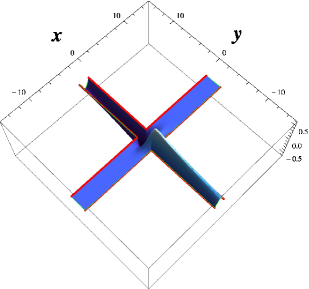
Figure 15: (color online) Wave function of the lowest even-odd state for $\beta=1.55$.

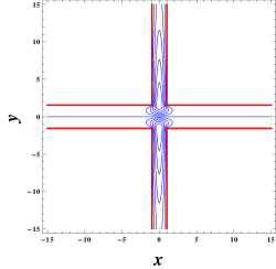
Figure 16: (color online) Wave function of the lowest even-odd state for $\beta=1.55$.

and a third region, where the wave function is still bound, but mainly localized in the horizontal arm (see for instances figs.17 and 18).

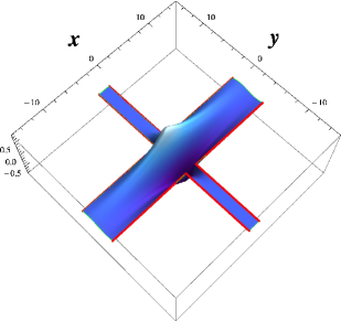
Figure 17: (color online) Wave function of the lowest even-odd state for $\beta=3$.

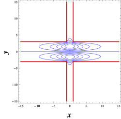
Figure 18: (color online) Wave function of the lowest even-odd state for $\beta=3$.

The ratio $E^{(\rm eo)}/E_{\rm TH}$ is plotted in Fig.19

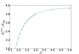
Figure 19: (color online) Ratio $E^{(\rm eo)}/E_{\rm TH}$ as a function of $\beta$ for the asymmetric cross; the solid line is the least squares fit $\left.E_{1}^{({\rm eo})}/E_{\rm TH}\right|^{\rm FIT}=3.96521+\frac{11.0968}{\beta^{7.38923}}-\frac{10.156}{\beta^{3.69462}}$.

and compared with the fit

$$\left.E_{1}^{({\rm eo})}/E_{\rm TH}\right|^{\rm FIT}=3.96521+\frac{11.0968}{\beta^{7.38923}}-\frac{10.156}{\beta^{3.69462}}.$$

As for the even-even state, this behavior is consistent with the survival of the bound state for $\beta\rightarrow\infty$.

In Fig. 20

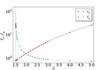
Figure 20: (color online) $\ell_{x}$ and $\ell_{y}$ as a function of $\beta$ for the lowest even-odd state of the asymmetric cross; the solid and dashed lines are the least squares fits $\left.\ell_{x}\right|^{\rm FIT}=0.129087\beta^{3.26312}+0.258401$ and $\left.\ell_{y}\right|^{\rm FIT}={0.604788}/({1-{2.16467}{\beta^{-1.86384}}})$. The vertical line corresponds to the critical value $\beta^{({\rm eo})}_{\star}=1.513$ where $\left.\ell_{y}\right|^{\rm FIT}$ is singular.

we plot $\ell_{x}$ and $\ell_{y}$ and compare with them the fits

$$\left.\ell_{x}\right|^{\rm FIT}=0.129087\beta^{3.26312}+0.258401$$

and

$$\left.\ell_{y}\right|^{\rm FIT}=\frac{0.604788}{1-\frac{2.16467}{\beta^{1.86384}}}.$$

The singularity of $\left.\ell_{y}\right|^{\rm FIT}$ is located at $\beta^{({\rm eo})}_{\star}=1.513$ (the vertical line in the plot) and represents the critical value where the bound state appears. Notice also that $\left.\ell_{x}\right|^{\rm FIT}\approx\left.\ell_{y}\right|^{\rm FIT}$ for $\beta=2$.

III.4 Odd-even state

In the case of the odd-even states we have not been able to find a bound state for any of the values of $\beta$ considered. Once again this behavior is consistent with our earlier predictions.

IV Conclusions

For years now, it has been verified theoretically, as well as experimentally, that the spectra of waves or quantum particles moving in several open two-dimensional systems could exhibit bound states. Since these bound states arise from the symmetry in the system, for applications it is important to find out how the perturbation of the given symmetry affects the corresponding spectrum.

In this paper we have shown that the question about the role of the symmetry of several setups can be answered by studying the simple problem of an effective one-dimensional quantum well. We support this conclusion by means of very accurate numerical solutions of the full Helmholtz equation with Dirichlet boundary conditions. It is worth to notice that the conclusions drawn from the simple problem are valid even for values of the ratio of the width of the crossing branches ($\beta$) for which the one-dimensional approximation not longer holds.

In particular, we have shown that the bound state of the symmetric cross persists for any finite value of $\beta$. A similar, but richer, behavior is obtained for the T-shaped configuration as the width of the vertical bar of the T tends to zero (i.e., $\beta\to\infty$): from $\beta=1$ up to $\beta_{\star}=1.513$ the wave function is unbound; above that critical value the wave function becomes bounded, but mainly localized in the vertical bar of the T; finally, if $\beta$ is still increased, the wave function remains bound, but mainly localized in the horizontal bar of the T. Of course, in any of these two setups, the bound state must dissapear as soon as the width of the decreasing branch reaches zero. Therefore, this seems to imply that adding just a very small perturbation on a very large one-dimensional quantum wire or waveguide may have a striking impact on the transport of charge carriers or waves along it.

The situation is different for the other two cases we analyzed. For the L-shaped configuration we have found that the bound state becomes unbounded at the critical value $\beta_{\star}=1.2279$ of the ratio of the width of the intersecting branches. Finally, for the T-shaped configuration no bound state arises when the width of the horizontal arm is decreased towards zero.

How strong are these effects as to be observable and appliable will depend on how strong is the departure of the actual experimental setup from the ideal configurations considered. Nevertheless, if the dependence on the symmetry found here is confirmed by future experiments, then it could be used as a switch-like mechanism for trapping and untrapping waves and charge carriers. This would give rise to a number of important applications.

V Acknowledgments

This research was supported by the Sistema Nacional de Investigadores (México). The work of CAT-E was also partially funded by PROMEP (México) under grant PROMEP/103.5/10/4948.

References

- (1) F. Ursell, Proc. Camb. Phil. Soc. 47, 348 (1951)
- (2) F. Ursell, Proc. R. Soc. Lond. A August 7, 214:79-97 (1952)
- (3) L. A. Weinstein, Open resonators and open waveguides, Sovietskoe Radio, Moscow, (1966) (in Russian, English traslation, Golem, Boulder, 1969)
- (4) H. Sakaki, Proc. Int. Symp. on Foundations of Quantum Mechanics in the Light of New Technology, eds. S. Kamefuchi et al., Phys. Soc. Japan (1984), pp. 94-110.
- (5) J. P. Carini, J. T. Londergan, D. P. Murdock, D. Trinkle, and C. S. Yung Phys. Rev. B 55, 9842–9851 (1997)
- (6) Londergan, J. T., J. P. Carini, and D. P. Murdock, Binding and Scattering in Two-dimensional Systems: Applications to Quantum Wires, Waveguides, and Photonic Crystals, Springer, Berlin, (1999).
- (7) M.L. Roukes, A. Scherer, S.J. Allen, Jr., H.G. Craighead, R.M. Ruthern, E.D. Beebe, and J.P. Harbison, Phys. Rev. Lett.59, 3011 (1988).
- (8) G. Timp, H.U. Baranger, P. deVegvar, J.E. Cunningham, R.E. Howard, R. Behringer, and P.M. Mankiewich, Phys. Rev. Lett.60, 2081 (1988).
- (9) Annino, G ; Cassettari, M ; Martinelli, M, ”A new concept of (open) TE011 cylindrical cavity”. Preprint: physics/0603154 (2006).
- (10) M.W.J.Bromley and B.D.Esry, Phys.Rev.A 68 043609 (2003).
- (11) S.- X. Qu and M. R. Geller, Phys. Rev. B 70, 85414 (2004)
- (12) Martin T. Hill, Yok-Siang Oei, Barry Smalbrugge, Youcai Zhu, Tjibbe de Vries, Peter J. van Veldhoven, Frank W. M. van Otten, Tom J. Eijkemans, Jaroslaw P. Turkiewicz, Huug de Waardt, Erik Jan Geluk, Soon-Hong Kwon, Yong-Hee Lee, Richard Nötzel, and Meint K. Smit, Nature Photonics 1, 589 - 594 (2007)
- (13) P. Exner and V. A. Zagrebnov, J. Phys. A: Math. Gen. 38 L463 (2005)
- (14) P. Exner, P. Šeba, M. Tater, and D. Vaněk, J. Math. Phys. 37, 4867 (1996)
- (15) G. Annino, H. Yashiro, M. Cassettari, M. Martinelli, Physical Review B, vol. 73, Issue 12, id. 125308 (2006)
- (16) R.L.Schult, D.G.Ravenall and H.W.Wyld, Phys.Rev.B 39 (1989) 5476-5479
- (17) Y. Avishai, D. Bessis, B.G. Giraud and G. Mantica, Phys.Rev.B 44 (1991) 8028-8034
- (18) P. Amore, F.M.Fernández and M. Rodriguez, ”Variational collocation with non uniform grids”, sent to J. Comp. Phys. (2011)
- (19) P. Amore, J. Phys. A 41, 265206 (2008)
- (20) L.N. Trefethen and T. Betcke, Recent advances in differential equations and mathematical physics: UAB International Conference on Differential Equations and Mathematical Physics, March 29-April 2, 2005, University of Alabama at Birmingham, 412, 297 (2006)
- (21) E.N. Bulgakov, P. Exner, K.N. Pichugin and A.F. Sadreev, Phys. Rev. B 66, 155109 (2002)
- (22) S. A. Nazarov, Acoustical Physics 56, 1004-1015 (2010)
- (23) P. Amore and D. Chowell, Journal of Sound and Vibration 329, 1362–1375 (2010)
- (24) D. L. Kaufman, I. Kosztin and K. Schulten, Am. J. Phys. 67, 133 (1999)