The PLUTO Code for Adaptive Mesh Computations in Astrophysical Fluid Dynamics

Abstract

We present a description of the adaptive mesh refinement (AMR) implementation of the PLUTO code for solving the equations of classical and special relativistic magnetohydrodynamics (MHD and RMHD). The current release exploits, in addition to the static grid version of the code, the distributed infrastructure of the CHOMBO library for multidimensional parallel computations over block-structured, adaptively refined grids. We employ a conservative finite-volume approach where primary flow quantities are discretized at the cell-center in a dimensionally unsplit fashion using the Corner Transport Upwind (CTU) method. Time stepping relies on a characteristic tracing step where piecewise parabolic method (PPM), weighted essentially non-oscillatory (WENO) or slope-limited linear interpolation schemes can be handily adopted. A characteristic decomposition-free version of the scheme is also illustrated. The solenoidal condition of the magnetic field is enforced by augmenting the equations with a generalized Lagrange multiplier (GLM) providing propagation and damping of divergence errors through a mixed hyperbolic/parabolic explicit cleaning step. Among the novel features, we describe an extension of the scheme to include non-ideal dissipative processes such as viscosity, resistivity and anisotropic thermal conduction without operator splitting. Finally, we illustrate an efficient treatment of point-local, potentially stiff source terms over hierarchical nested grids by taking advantage of the adaptivity in time. Several multidimensional benchmarks and applications to problems of astrophysical relevance assess the potentiality of the AMR version of PLUTO in resolving flow features separated by large spatial and temporal disparities.

1. Introduction

Theoretical advances in modern astrophysics have largely benefited from computational models and techniques that have been improved over the past decades. In the field of gasdynamics, shock-capturing schemes represent the current establishment for reliable numerical simulations of high Mach-number, possibly magnetized flows in Newtonian or relativistic regimes. As increasingly more sophisticated methods developed, a number of computer codes targeting complex physical aspects to various degrees have now become available to the community. In the field of magnetohydrodynamics (MHD), examples worth of notice are AstroBEAR (Cunningham et al., 2009), Athena (Stone et al., 2008; Skinner & Ostriker, 2010), BATS-R-US (Tóth et al., 2011), ECHO (Del Zanna et al., 2007), FLASH (Fryxell et al., 2000), NIRVANA (Ziegler, 2008), PLUTO (Mignone et al., 2007), RAMSES (Teyssier, 2002; Fromang et al., 2006) and VAC (Tóth, 1996; van der Holst et al., 2008). Some of these implementions provide additional capabilities that can approach the solution of the equations in the relativistic regimes: AMRVAC and PLUTO for special relativistic hydro, while the ECHO code allows to handle general relativistic MHD with a fixed metric. Other frameworks were specifically designed for special or general relativistic purposes, e.g. the RAM code (Zhang & MacFadyen, 2006), HARM (Gammie et al., 2003) and RAISHIN (Mizuno et al., 2006).

In some circumstances, adequate theoretical modeling of astrophysical scenarios may become extremely challenging since great disparities in the spatial and temporal scales may simultaneously arise in the problem of interest. In these situations a static grid approach may become quite inefficient and, in the most extreme cases, the amount of computational time can make the problem prohibitive. Typically, such conditions occur when the flow dynamics exhibit very localized features that evolve on a much shorter scale when compared to the rest of the computational domain. To overcome these limitations, one possibility is to change or adapt the computational grid dynamically in space and time so that the features of interest can be adequately captured and resolved. Adaptive mesh refinement (AMR) is one such technique and can lead, for a certain class of problems, to a considerable speed up. Some of the aforementioned numerical codes provide AMR implementations through a variety of different approaches. Examples worth of notice are the patch-based block-structured approach of Berger & Oliger (1984); Berger & Colella (1989) (e.g. ASTROBEAR), the fully-octree approach described in Dezeeuw & Powell (1993); Khokhlov (1998) (e.g. RAMSES) or the block-based octree of MacNeice et al. (2000) (e.g. FLASH) and Keppens et al. (2003); van der Holst & Keppens (2007) (e.g. BATS-R-US, AMRVAC).

The present work focuses on the block-structured AMR implementation in the PLUTO code and its application to computational astrophysical gasdynamics. PLUTO is a Godunov-type code providing a flexible and versatile modular computational framework for the solution of the equations of gasdynamics under different regimes (e.g., classical/relativistic fluid dynamics, Euler/MHD). A comprehensive description of the code design and implementation may be found, for the static grid version, in Mignone et al. (2007) (paper I henceforth). Recent additions to the code include a relativistic version of the HLLD Riemann solver (Mignone et al., 2009), high-order finite difference schemes (Mignone et al., 2010) and optically thin radiative losses with a non-equilibrium chemical network (Teşileanu et al., 2008). Here we further extend the code description and show its performance on problems requiring significant usage of adaptively refined nested grids. PLUTO takes advantage of the CHOMBO library that provides a distributed infrastructure for parallel computations over block-structured adaptively refined grids. The choice of block-structured AMR (as opposed to octree) is justified by the need of exploiting the already implemented modular skeleton introducing the minimal amount of modification and, at the same time, maximizing code re-usability.

The current AMR implementation leans on the Corner-Transport-Upwind (CTU, Colella, 1990) method of Mignone & Tzeferacos (2010) (MT henceforth) in which a conservative finite volume discretization is adopted to evolve zone averages in time. The scheme is dimensionally unsplit, second-order accurate in space and time and can be directly applied to relativistic MHD as well. Spatial reconstruction can be carried out in primitive or characteristic variables using high-order interpolation schemes such as the piecewise parabolic method (PPM, Colella & Woodward, 1984), weighted essentially non-oscillatory (WENO) or linear Total Variation Diminishing (TVD) limiting. The divergence-free constraint of magnetic field is enforced via a mixed hyperbolic/parabolic correction of Dedner et al. (2002) that avoids the computational cost associated with an elliptic cleaning step, and the scrupulous treatment of staggered fields demanded by constrained transport algorithms (Balsara, 2004). As such, this choice provides a convenient first step in porting a considerable fraction of the static grid implementation to the AMR framework. Among the novel features, we also show how to extend the time-stepping scheme to include dissipative terms describing viscous, resistive and thermally conducting flows. Besides, we propose a novel treatment for efficiently computing the time-step in presence of cooling and/or reacting flows over hierarchical block-structured grids.

The paper is structured as follows. In Section 2 we overview the relevant equations while in Section 3 we describe the integration scheme used on the single patch. In Section 4 an overview of the block-structured AMR strategy as implemented in CHOMBO is given. Sections 5 and 6 show the code performance on selected multidimensional test problems and astrophysical applications in classical and relativistic MHD, respectively. Finally, in Section 7 we summarize the main results of our work.

2. Relevant Equations

The PLUTO code has been designed for the solution of nonlinear systems of conservative partial differential equations of the mixed hyperbolic/parabolic type. In the present context we will focus our attention on the equations of single-fluid magnetohydrodynamics, both in the Newtonian (MHD) and special relativistic (RMHD) regimes.

2.1. MHD equations

We consider a Newtonian fluid with density $\rho$, velocity $\mathbf{v}=(v_{x},v_{y},v_{z})$ and magnetic induction $\mathbf{B}=(B_{x},B_{y},B_{z})$ and write the single fluid MHD equations as

$$\begin{array}[]{lcl}\displaystyle\frac{\partial\rho}{\partial t}+\nabla\cdot\left(\rho\mathbf{v}\right)&=&0\,,\\ \vskip 6.0pt plus 2.0pt minus 2.0pt\cr\displaystyle\frac{\partial\mathbf{(\rho\mathbf{v})}}{\partial t}+\nabla\cdot\left[\rho\mathbf{v}\mathbf{v}^{T}-\mathbf{B}\mathbf{B}^{T}\right]+\nabla p_{t}&=&\nabla\cdot\mathsf{\tau}+\rho\mathbf{g}\,,\\ \vskip 6.0pt plus 2.0pt minus 2.0pt\cr\displaystyle\frac{\partial\cal E}{\partial t}+\nabla\cdot\left[\left({\cal E}+p_{t}\right)\mathbf{v}-\left(\mathbf{v}\cdot\mathbf{B}\right)\mathbf{B}\right]&=&\nabla\cdot\mathsf{\Pi}_{\cal E}-\Lambda+\rho\mathbf{v}\cdot\mathbf{g}\,,\\ \vskip 6.0pt plus 2.0pt minus 2.0pt\cr\displaystyle\frac{\partial\mathbf{B}}{\partial t}-\nabla\times\left(\mathbf{v}\times\mathbf{B}\right)&=&-\nabla\times\left(\mathsf{\eta}\mathbf{J}\right)\,,\end{array}$$ (1)

where $p_{t}=p+\mathbf{B}^{2}/2$ is the total (thermal+magnetic) pressure, ${\cal E}$ is the total energy density, $\mathbf{g}$ is the gravitational acceleration term and $\Lambda$ accounts for optically thin radiative losses or heating. Divergence terms on the right-hand side account for dissipative physical processes and are described in detail in Section 2.1.1. Proper closure is provided by choosing an equation of state (EoS) which, for an ideal gas, allows to write the total energy density as

$${\cal E}=\frac{p}{\Gamma-1}+\frac{1}{2}\rho\mathbf{v}^{2}+\frac{1}{2}\mathbf{B}^{2}\,,$$ (2)

with $\Gamma$ being the specific heat ratio. Alternatively, by adopting a barotropic or an isothermal EoS, the energy equation can be discarded and one simply has, respectivelty, $p=p(\rho)$ or $p=c_{s}^{2}\rho$ (where $c_{s}$ is the constant speed of sound).

Chemical species and passive scalars are advected with the fluid and are described in terms of their number fraction $X_{\alpha}$ where $\alpha=1,\cdots,N_{\rm ions}$ label the particular ion. They obey non-homogeneous transport equations of the form

$$\frac{\partial(\rho X_{\alpha})}{\partial t}+\nabla\cdot\left(\rho X_{\alpha}\mathbf{v}\right)=\rho S_{\alpha}\,,$$ (3)

where the source term $S_{\alpha}$ describes the coupling between different chemical elements inside the reaction network (see for instance Teşileanu et al., 2008).

2.1.1 Non-Ideal Effects

Non-ideal effects due to dissipative processes are described by the differential operators included on the right-hand side of Eq. (1). Viscous stresses may be included through the viscosity tensor $\mathsf{\tau}$ defined by

$$\mathsf{\tau}=\rho\nu\left[\nabla\mathbf{v}+(\nabla\mathbf{v})^{T}-\frac{2}{3}\mathsf{I}\nabla\cdot\mathbf{v}\right]\,,$$ (4)

where $\nu$ is the kinematic viscosity and $\mathsf{I}$ is the identity matrix. Similarly, magnetic resistivity is accounted for by prescribing the resistive $\eta$ tensor (diagonal). Dissipative terms contribute to the net energy balance through the additional flux $\mathsf{\Pi}_{\cal E}$ appearing on the right hand side of Eq. (1):

$$\mathsf{\Pi}_{\cal E}=\mathbf{F}_{c}+\mathbf{v}\cdot\mathsf{\tau}-\mathsf{\eta}\cdot\mathbf{J}\times\mathbf{B}\,,$$ (5)

where the different terms give the energy flux contributions due to, respectively, thermal conductivity, viscous stresses and magnetic resistivity.

The thermal conduction flux $\mathbf{F}_{c}$ smoothly varies between classical and saturated regimes and reads:

$$\mathbf{F}_{c}=\frac{q}{|\mathbf{F}_{\rm class}|+q}\mathbf{F}_{\rm class}$$ (6)

where $q=5\phi\rho c_{\rm iso}^{3}$ is the magnitude of the saturated flux (Cowie & McKee, 1977), $\phi$ is a parameter of order unity accounting for uncertainties in the estimate of $q$, $c_{\rm iso}$ is the isothermal speed of sound and

$$\mathbf{F}_{\rm class}=\kappa_{\parallel}\hat{\mathbf{b}}\Big{(}\hat{\mathbf{b}}\cdot\nabla T\Big{)}+\kappa_{\perp}\left[\nabla T-\hat{\mathbf{b}}\Big{(}\hat{\mathbf{b}}\cdot\nabla T\Big{)}\right]$$ (7)

is the classical heat flux with conductivity coefficients $\kappa_{\parallel}$ and $\kappa_{\perp}$ along and across the magnetic field lines, respectively (Orlando et al., 2008). Indeed, the presence of a partially ordered magnetic field introduces a large anisotropic behavior by channeling the heat flux along the field lines while suppressing it in the transverse direction (here $\hat{\mathbf{b}}=\mathbf{B}/|\mathbf{B}|$ is a unit vector along the field line). We point out that, in the classical limit $q\to\infty$, thermal conduction is described by a purely parabolic operator and flux discretization follows standard finite difference. In the saturated limit ($|\nabla T|\to\infty$), on the other hand, the equation becomes hyperbolic and thus an upwind discretization of the flux is more appropriate (Balsara et al., 2008). This is discussed in more detail in Appendix A.

2.2. Relativistic MHD equations

A (special) relativistic extension of the previous equations requires the solution of energy-momentum and number density conservation. Written in divergence form we have

$$\begin{array}[]{lcl}\displaystyle\frac{\partial(\rho\gamma)}{\partial t}+\nabla\cdot\left(\rho\gamma\mathbf{v}\right)&=&0\,,\\ \vskip 6.0pt plus 2.0pt minus 2.0pt\cr\displaystyle\frac{\partial\mathbf{m}}{\partial t}+\nabla\cdot\left[w\gamma^{2}\mathbf{v}\mathbf{v}-\mathbf{B}\mathbf{B}-\mathbf{E}\mathbf{E}\right]+\nabla p_{t}&=&0\,,\\ \vskip 6.0pt plus 2.0pt minus 2.0pt\cr\displaystyle\frac{\partial\mathbf{B}}{\partial t}-\nabla\times\left(\mathbf{v}\times\mathbf{B}\right)&=&0\,,\\ \vskip 6.0pt plus 2.0pt minus 2.0pt\cr\displaystyle\frac{\partial\cal E}{\partial t}+\nabla\cdot\left(\mathbf{m}-\rho\gamma\mathbf{v}\right)&=&0\,,\end{array}$$ (8)

where $\rho$ is the rest-mass density, $\gamma$ the Lorentz factor, velocities are given in units of the speed of light ($c=1$) and the fluid momentum $\mathbf{m}$ accounts for matter and electromagnetic terms: $\mathbf{m}=w\gamma^{2}\mathbf{v}+\mathbf{E}\times\mathbf{B}$, where $\mathbf{E}=-\mathbf{v}\times\mathbf{B}$ is the electric field and $w$ is the gas enthalpy. Total pressure and energy include thermal and magnetic contributions and can be written as

$$p_{t}=p+\frac{\mathbf{B}^{2}+\mathbf{E}^{2}}{2}\,,\quad{\cal E}=w\gamma^{2}-p+\frac{\mathbf{B}^{2}+\mathbf{E}^{2}}{2}-\rho\gamma\,.$$ (9)

Finally, the gas enthalpy $w$ is related to $\rho$ and $p$ via an equation of state which can be either the ideal gas law,

$$w=\rho+\frac{\Gamma p}{\Gamma-1}\,,$$ (10)

or the TM (Taub-Mathews, Mathews, 1971) equation of state

$$w=\frac{5}{2}p+\sqrt{\frac{9}{4}p^{2}+\rho^{2}}\,,$$ (11)

which provides an analytic approximation of the Synge relativistic perfect gas (Mignone & McKinney, 2007).

A relativistic formulation of the dissipative terms will not be presented here and will be discussed elsewhere.

2.3. General Quasi-Conservative Form

In the following we shall adopt an orthonormal system of coordinates specified by the unit vectors $\hat{\mathbf{e}}_{d}$ ($d$ is used to label the direction, e.g. $d=\{x,y,z\}$ in Cartesian coordinates) and conveniently assume that conserved variables $\mathbf{U}=(\rho,\rho\mathbf{v},{\cal E},\mathbf{B},\rho X_{\alpha})$ - for the MHD equations - and $\mathbf{U}=(\rho\gamma,\mathbf{m},{\cal E},\mathbf{B})$ - for RMHD - satisfy the following hyperbolic/parabolic partial differential equations

$$\frac{\partial\mathbf{U}}{\partial t}+\nabla\cdot\mathsf{F}=\nabla\cdot\mathsf{\Pi}+\mathbf{S}_{p}\,,$$ (12)

where $\mathsf{F}$ and $\mathsf{\Pi}$ are, respectively, the hyperbolic and parabolic flux tensors. The source term $\mathbf{S}_{p}$ is a point-local source term which accounts for body forces (such as gravity), cooling, chemical reactions and the source term for the scalar multiplier (see Eq. 14 below). We note that equations containing curl or gradient operators can always be cast in this form by suitable vector identities. For instance, the projection of $\nabla\times\mathbf{E}$ in the coordinate direction given by the unit vector $\hat{\mathbf{e}}_{d}$ can be re-written as

$$(\nabla\times\mathbf{E})\cdot\hat{\mathbf{e}}_{d}\equiv\nabla\cdot\left(\mathbf{E}\times\hat{\mathbf{e}}_{d}\right)+\mathbf{E}\cdot\left(\nabla\times\hat{\mathbf{e}}_{d}\right)\,,$$ (13)

where the second term on the right hand side should be included as an additional source term in Eq. (12) whenever different from zero (e.g. in cylindrical geometry). Similarly one can re-write the gradient operator as $\nabla p=\nabla\cdot\left(\mathsf{I}p\right)$.

Several algorithms employed in PLUTO are best implemented in terms of primitive variables, $\mathbf{V}=(\rho,\mathbf{v},\mathbf{B},p)$. In the following we shall assume a one-to-one mapping between the two sets of variables, provided by appropriate conversion functions, that is $\mathbf{V}=\mathbf{V}(\mathbf{U})$ and $\mathbf{U}=\mathbf{U}(\mathbf{V})$.

3. Single Patch Numerical Integration

PLUTO approaches the solution of the previous sets of equations using either finite-volume (FV) or finite-difference (FD) methods both sharing a flux-conservative discretization where volume averages (for the former) or point values (for the latter) of the conserved quantities are advanced in time. The implementation is based on the well-established framework of Godunov type, shock-capturing schemes where an upwind strategy (usually a Riemann solver) is employed to compute fluxes at zone faces. For the present purposes, we shall focus on the FV approach where volume-averaged primary flow quantities (e.g. density, momentum and energy) retain a zone-centered discretization. However, depending on the strategy chosen to control the solenoidal constraint, the magnetic field can evolve either as a cell-average or as a face-average quantity (using Stoke’s theorem). As described in paper I, both approaches are possible in PLUTO by choosing between Powell’s eight wave formulation or the constrained transport (CT) method, respectively.

A third, cell-centered approach based on the generalized Lagrange multiplier (GLM) formulation of Dedner et al. (2002) has recently been introduced in PLUTO and a thorough discussion as well as a direct comparison with CT schemes can be found in the recent work by MT. The GLM formulation easily builds in the context of MHD and RMHD equations by introducing an additional scalar field $\psi$ which couples the divergence constraint to Faraday’s law according to

$$\left\{\begin{array}[]{lcl}\displaystyle\frac{\partial\mathbf{B}}{\partial t}-\nabla\times\left(\mathbf{v}\times\mathbf{B}\right)+\nabla\psi&=&0\,,\\ \vskip 6.0pt plus 2.0pt minus 2.0pt\cr\displaystyle\frac{\partial\psi}{\partial t}+c_{h}^{2}\nabla\cdot\mathbf{B}&=&\displaystyle-\frac{c_{h}^{2}}{c_{p}^{2}}\psi\,,\end{array}\right.$$ (14)

where $c_{h}$ is the (constant) speed at which divergence errors are propagated while $c_{p}$ is a constant controlling the rate at which monopoles are damped. The remaining equations are not changed and the conservative character is not lost. Owing to its ease of implementation, we adopt the GLM formulation as a convenient choice in the development of a robust AMR framework for Newtonian and relativistic MHD flows.

3.1. Fully Unsplit Time Stepping

The system of conservation laws is advanced in time using the Corner-Transport-Upwind (CTU, Colella, 1990) method recently described by MT. Here we outline the algorithm in a more concise manner and extend its applicability in presence of parabolic (diffusion) terms and higher order reconstruction. Although the algorithms illustrated here are explicit in time, we will also consider the description of more sophisticated and effective approaches for the treatment of parabolic operators in a forthcoming paper.

We shall assume hereafter an equally-spaced grid with computational cells centered in $(x_{i},y_{j},z_{k})$ having size $\Delta x\times\Delta y\times\Delta z$. For the sake of exposition, we omit the integer subscripts $i,j$ or $k$ when referring to the cell center and only keep the half-increment notation in denoting face values, e.g., $\mathbf{F}_{d,\pm}\equiv\mathbf{F}_{y,i,j+\frac{1}{2},k}$ when $d=y$. Following Mignone et al. (2007), we use $\Delta{\cal V}$ and $A_{d,\pm}$ to denote, respectively, the cell volume and areas of the lower and upper interfaces orthogonal to $\hat{\mathbf{e}}_{d}$.

An explicit second-order accurate discretization of Eqns. (12), based on a time-centered flux computation, reads

$$\bar{\mathbf{U}}^{n+1}=\bar{\mathbf{U}}^{n}+\Delta t^{n}\sum_{d}\left(\boldsymbol{\cal L}_{H,d}^{n+\frac{1}{2}}+\boldsymbol{\cal L}_{P,d}^{n+\frac{1}{2}}\right)\,,$$ (15)

where $\bar{\mathbf{U}}$ is the volume-averaged array of conserved values inside the cell $(i,j,k)$, $\Delta t^{n}$ is the explicit time step whereas $\boldsymbol{\cal L}_{H,d}$ and $\boldsymbol{\cal L}_{P,d}$ are the increment operators corresponding to the hyperbolic and parabolic flux terms, respectively:

$$\boldsymbol{\cal L}_{H,d}^{n+\frac{1}{2}} = -\frac{A_{d,+}\mathbf{F}^{n+\frac{1}{2}}_{d,+}-A_{d,-}\mathbf{F}^{n+\frac{1}{2}}_{d,-}}{\Delta{\cal V}_{d}}+\hat{\mathbf{S}}_{d}^{n+\frac{1}{2}}\,,\quad$$ (16)

$$\boldsymbol{\cal L}_{P,d}^{n+\frac{1}{2}} = \frac{A_{d,+}\boldsymbol{\Pi}^{n+\frac{1}{2}}_{d,+}-A_{d,-}\boldsymbol{\Pi}^{n+\frac{1}{2}}_{d,-}}{\Delta{\cal V}_{d}}\,,$$ (17)

In the previous expression $\mathbf{F}_{d,\pm}$ and $\boldsymbol{\Pi}_{d,\pm}$ are, respectively, right ($+$) and left ($-$) face- and time-centered approximations to the hyperbolic and parabolic flux components in the direction of $\hat{\mathbf{e}}_{d}$. The source term $\hat{\mathbf{S}}_{d}$ represents the directional contribution to the total source vector $\sum\hat{\mathbf{S}}_{d}\equiv\hat{\mathbf{S}}_{\rm body}+\hat{\mathbf{S}}_{\rm geo}$ including body forces and geometrical terms implicitly arising when differentiating the tensor flux on a curvilinear grid. Cooling, chemical reaction terms and the source term in Eq. 14 (namely $(c_{h}^{2}/c_{p}^{2})\psi$) are treated separately in an operator-split fashion.

The computation of $\mathbf{F}_{d,\pm}$ requires solving, at cell interfaces, a Riemann problem between time-centered adjacent discontinuous states, i.e.

$$\begin{array}[]{lcl}\mathbf{F}^{n+\frac{1}{2}}_{x,i+\frac{1}{2}}&=&{\cal R}\left(\mathbf{U}^{n+\frac{1}{2}}_{i,+},\mathbf{U}^{n+\frac{1}{2}}_{i+1,-}\right)\,,\\ \vskip 6.0pt plus 2.0pt minus 2.0pt\cr\mathbf{F}^{n+\frac{1}{2}}_{y,j+\frac{1}{2}}&=&{\cal R}\left(\mathbf{U}^{n+\frac{1}{2}}_{j,+},\mathbf{U}^{n+\frac{1}{2}}_{j+1,-}\right)\,,\\ \vskip 6.0pt plus 2.0pt minus 2.0pt\cr\mathbf{F}^{n+\frac{1}{2}}_{z,k+\frac{1}{2}}&=&{\cal R}\left(\mathbf{U}^{n+\frac{1}{2}}_{k,+},\mathbf{U}^{n+\frac{1}{2}}_{k+1,-}\right)\,,\end{array}$$ (18)

where ${\cal R}(\cdot,\cdot)$ is the numerical flux resulting from the solution of the Riemann problem. With PLUTO , different Riemann solvers may be chosen at runtime depending on the selected physical module (see Paper I): Rusanov (Lax-Friedrichs), HLL, HLLC and HLLD are common to both classical and relativistic MHD modules while the Roe solver is available for hydro and MHD. The input states in the Eq. (18) are obtained by first carrying an evolution step in the normal direction, followed by correcting the resulting values with a transverse flux gradient. This yields the corner-coupled states which, in absence of parabolic terms (i.e. when $\mathsf{\Pi}=\mathsf{0}$), are constructed exactly as illustrated by MT. For this reason, we will not repeat it here.

When $\mathsf{\Pi}\neq 0$, on the other hand, we adopt a slightly different formulation that does not require any change in the computational stencil. At constant $x$-faces, for instance, we modify the corner-coupled states to

$$\mathbf{U}^{n+\frac{1}{2}}_{i,\pm}=\mathbf{U}^{*}_{i,\pm}+\frac{\Delta t^{n}}{2}\left[\sum_{d\neq x}\boldsymbol{\cal L}_{H,d}^{n}+\sum_{d}\boldsymbol{\cal L}_{P,d}^{n}\right]\,,$$ (19)

where, using Godunov’s first-order method, we compute for example

$$\mathbf{F}^{n}_{y,j+\frac{1}{2}}={\cal R}(\bar{\mathbf{U}}^{n}_{j},\bar{\mathbf{U}}^{n}_{j+1})\,,$$ (20)

i.e., by solving a Riemann problem between cell-centered states. States at constant $y$ and $z$-faces are constructed in a similar manner. The normal predictors $\mathbf{U}^{*}_{\pm}$ can be obtained either in characteristic or primitive variables as outlined in Section 3.2 and Section 3.3, respectively. Parabolic (dissipative) terms are discretized in a flux-conservative form using standard central finite difference approximations to the derivatives. For any term in the form $\Pi=g(\mathbf{U})\partial_{x}f(\mathbf{U)}$, for instance, we evaluate the right interface flux appearing in Eq. (17) with the second-order accurate expression

$$\Pi_{x,+}\approx g\left(\frac{\mathbf{U}_{i}+\mathbf{U}_{i+1}}{2}\right)\frac{\displaystyle f\left(\mathbf{U}_{i+1}\right)-f\left(\mathbf{U}_{i}\right)}{\Delta x}\,,$$ (21)

and similarly for the other directions (a similar approach is used by Tóth et al., 2008). We take the solution available at the cell center at $t=t^{n}$ in Eq. (19) and at the half time step $n+\frac{1}{2}$ in Eq. (15). For this latter update, time- and cell-centered conserved quantities may be readily obtained as

$$\mathbf{U}^{n+\frac{1}{2}}=\bar{\mathbf{U}}^{n}+\frac{\Delta t^{n}}{2}\sum_{d}\left(\boldsymbol{\cal L}_{H,d}^{n}+\boldsymbol{\cal L}_{P,d}^{n}\right)\,.$$ (22)

The algorithm requires a total of $6$ solutions to the Riemann problems per zone per step and it is stable under the Courant-Friedrichs-Levy (CFL) condition $C_{a}\leq 1$ (in 2D) or $C_{a}\leq 1/2$ (in 3D), where

$$C_{a}=\Delta t^{n+1}\max_{ijk}\left[\max_{d}\left(\frac{\lambda^{\max}_{d}}{\Delta x_{d}}\right)+\sum_{d}\frac{2{\cal D}^{\max}_{d}}{\Delta x_{d}^{2}}\right]$$ (23)

is the CFL number, $\lambda^{\max}_{d}$ and ${\cal D}^{\max}_{d}$ are the (local) largest signal speed and diffusion coefficient in the direction given by $d=\{x,y,z\}$, respectively. Equation (23) is used to retrieve the time step $\Delta t^{n+1}$ for the next time level if no cooling or reaction terms are present. Otherwise we further limit the time step so that the relative change in pressure and chemical species remains below a certain threshold $\epsilon_{c}$:

$$\Delta t^{n+1}\to\min\left[\Delta t^{n+1},\frac{\epsilon_{c}\Delta t^{n}}{\max(|\delta p/p|,|\delta X_{\kappa}|)}\right]$$ (24)

where $\delta p/p$ and $\delta X_{\kappa}$ are the maximum fractional variations during the source step (Teşileanu et al., 2008). We note that the time step limitation given by equation (24) does not depend on the mesh size and can be estimated on unrefined cells only. This allows to take full advantage of the adaptivity in time as explained in Section 4.2.

3.2. Normal predictors in characteristic variables

The computation of the normal predictor states can be carried out in characteristic variables by projecting the vector $\mathbf{V}$ of primitive variables onto the left eigenvectors $\mathbf{l}^{\kappa}_{i}\equiv\mathbf{l}^{\kappa}(\mathbf{V}_{i})$ of the primitive system. Specializing to the x direction:

$$w^{\kappa}_{i,l}=\mathbf{l}_{i}^{\kappa}\cdot\mathbf{V}_{i+l}\,,\quad l=-S,\cdots,S\,,$$ (25)

where $\kappa=1,\cdots,N_{\rm wave}$ labels the characteristic wave with speed $\lambda^{\kappa}$ and the projection extends to all neighboring zones required by the interpolation stencil of width $2S+1$. The employment of characteristic fields rather than primitive variables requires the additional computational cost associated with the full spectral decomposition of the primitive form of the equations. Nevertheless, it has shown to produce better-behaved solutions for highly nonlinear problems, notably for higher order methods.

For each zone $i$ and characteristic field $\kappa$, we first interpolate $w^{\kappa}_{i,l}$ to obtain $w^{\kappa}_{i,\pm}$, that is, the rightmost ($+$) and leftmost ($-$) interface values from within the cell. The interpolation can be carried out using either fourth-, third- or second-order piecewise reconstruction as outlined later in this section.

Extrapolation in time to $t^{n}+\Delta t^{n}/2$ is then carried out by using an upwind selection rule that discards waves not reaching a given interface in $\Delta t/2$. The result of this construction, omitting the $\kappa$ index for the sake of exposition, reads

$$w^{*}_{i,+}=w^{\rm ref}_{i,+}+\beta_{+}\left\{w_{i,+}-\frac{\nu}{2}\left[\delta w_{i}+\delta^{2}w_{i}\left(3-2\nu\right)\right]-w^{\rm ref}_{i,+}\right\}\,,$$ (26)

$$w^{*}_{i,-}=w^{\rm ref}_{i,-}+\beta_{-}\left\{w_{i,-}-\frac{\nu}{2}\left[\delta w_{i}-\delta^{2}w_{i}\left(3+2\nu\right)\right]-w^{\rm ref}_{i,-}\right\}\,,$$ (27)

where $\nu\equiv\lambda\Delta t/\Delta x$ is the Courant number of the $\kappa$-th wave, $\beta_{\pm}=(1\pm{\rm sign}(\nu))/2$, whereas $\delta w_{i}$ and $\delta^{2}w_{i}$ are defined by

$$\delta w_{i}=w_{i,+}-w_{i,-}\,,\qquad\delta^{2}w_{i}=w_{i,+}-2w_{i}+w_{i,-}\,.$$ (28)

The choice of the reference state $w^{\rm ref}_{i,\pm}$ is somewhat arbitrary and one can simply set $w^{\rm ref}_{i,\pm}=w_{i,0}$ (Rider et al., 2007) which has been found to work well for flows containing strong discontinuities. Alternatively, one can use the original prescription (Colella & Woodward, 1984)

$$w^{\rm ref}_{i,+}=w_{i,+}-\frac{\nu_{\max}}{2}\left[\delta w_{i}+\delta^{2}w_{i}\left(3-2\nu_{\max}\right)\right]\,,$$ (29)

$$w^{\rm ref}_{i,-}=w_{i,-}-\frac{\nu_{\min}}{2}\left[\delta w_{i}-\delta^{2}w_{i}\left(3+2\nu_{\min}\right)\right]\,,$$ (30)

where $\nu_{\max}=\max(0,\max_{\kappa}(\nu_{\kappa}))$ and $\nu_{\min}=\min(0,\min_{\kappa}(\nu_{\kappa}))$ are chosen so as to minimize the size of the term susceptible to characteristic limiting (Colella & Woodward, 1984; Miller & Colella, 2002; Mignone et al., 2005). However we note that, in presence of smooth flows, both choices may reduce the formal second order accuracy of the scheme since, in the limit of small $\Delta t$, contributions carried by waves not reaching a zone edge are not included when reconstructing the corresponding interface value (Stone et al., 2008). In these situations, a better choice is to construct the normal predictors without introducing a specific reference state or, equivalently, by assigning $w^{\rm ref}_{i,\pm}=w_{i,\pm}$ in Eq. (26) and (27).

The time-centered interface values obtained in characteristic variables through Eq. (26) and (27) are finally used as coefficients in the right-eigenvector expansion to recover the primitive variables:

$$\mathbf{V}^{*}_{i,\pm}=\sum_{\kappa}w^{\kappa,*}_{i,\pm}\mathbf{r}^{\kappa}_{i}+\frac{\Delta t^{n}}{2}\left(\mathbf{S}_{g,i}^{n}+\mathbf{S}_{B_{x},i}^{n}\frac{\Delta B_{x}}{\Delta x}+\mathbf{S}_{\psi,i}^{n}\frac{\Delta\psi}{\Delta x}\right)\,,$$ (31)

where $\mathbf{r}^{\kappa}$ is the right eigenvector associated to the $\kappa$-th wave, $\mathbf{S}_{g}$ is a source term accounting for body forces and geometrical factors while $\mathbf{S}_{\rm B_{x}}$ and $\mathbf{S}_{\rm\psi}$ arise from calculating the interface states in primitive variables rather than conservative ones and are essential for the accuracy of the scheme in multiple dimensions. See MT for a detailed discussion on the implementation of these terms.

As mentioned, the construction of the left and right interface values can be carried out using different interpolation techniques. Although some of the available options have already been presented in the original paper (Mignone et al., 2007), here we briefly outline the implementation details for three selected schemes providing (respectively) fourth-, third- and second-order spatially accurate interface values in the limit of vanishing time step. Throughout this section we will make frequent usage of the undivided differences of characteristic variables (25) such as

$$\Delta w_{i,+\frac{1}{2}}=w_{i,+1}-w_{i,0}\,,\quad\Delta w_{i,-\frac{1}{2}}=w_{i,0}-w_{i,-1}\,.$$ (32)

for the $i$-th zone.

Piecewise Parabolic Method

The original PPM reconstruction by Colella & Woodward (1984) (see also Miller & Colella, 2002) can be directly applied to characteristic variables giving the following fourth-order limited interface values:

$$w_{i,\pm}=\frac{w_{i,0}+w_{i,\pm 1}}{2}\mp\frac{\overline{\Delta w}_{i,\pm 1}-\overline{\Delta w}_{i,0}}{6}\,,$$ (33)

where slope limiting is used to ensure that $w_{i,\pm}$ are bounded between $w_{i}$ and $w_{i\pm 1}$:

$$\overline{\Delta w}_{i,0}={\rm mm}\left[\frac{\Delta w_{i,+\frac{1}{2}}+\Delta w_{i,-\frac{1}{2}}}{2},2{\rm mm}\left(\Delta w_{i,-\frac{1}{2}},\Delta w_{i,+\frac{1}{2}}\right)\right]$$ (34)

and

$${\rm mm}(a,b)=\frac{\rm{sign}(a)+\rm{sign}(b)}{2}\min\left(|a|,|b|\right)\,,$$ (35)

is the MinMod function. The original interface values defined by Eq. (33) must then be corrected to avoid the appearance of local extrema. By defining $\delta_{\pm}=w_{i,\pm}-w_{i,0}$, we further apply the following parabolic limiter

$$\delta_{\pm}=\left\{\begin{array}[]{ll}0&\quad\textrm{if}\quad\delta_{+}\delta_{-}>0\\ \vskip 6.0pt plus 2.0pt minus 2.0pt\cr-2\delta_{\mp}&\quad\textrm{if}\quad|\delta_{\pm}|\geq 2|\delta_{\mp}|\,,\end{array}\right.$$ (36)

where the first condition flattens the distribution when $w_{i,0}$ is a local maximum or minimum whereas the second condition prevents the appearance of an extremum in the parabolic profile. Once limiting has been applied, the final interface values are obtained as

$$w_{i,\pm}=w_{i,0}+\delta_{\pm}\,.$$ (37)

In some circumstances, we have found that further application of the parabolic limiter (36) to primitive variables may reduce oscillations.

Third-order improved WENO

As an alternative to the popular TVD limiters, the third-order improved weighted essentially non-oscillatory (WENO) reconstruction proposed by Yamaleev & Carpenter (2009) (see also Mignone et al., 2010) may be used. The interpolation still employs a three-point stencil but provides a piecewise parabolic profile that preserves the accuracy at smooth extrema, thus avoiding the well known clipping of classical second-order TVD limiters. Left and right states are recovered by a convex combination of $2^{\rm nd}$ order interpolants into a weighted average of order $3$. The nonlinear weights are adjusted by the local smoothness of the solution so that essentially zero weights are given to non smooth stencils while optimal weights are prescribed in smooth regions. In compact notation:

$$\begin{array}[]{ccc}w_{i,+}&=&\displaystyle w_{i,0}+\frac{a_{+}\Delta w_{i,+\frac{1}{2}}+\frac{1}{2}a_{-}\Delta w_{i,-\frac{1}{2}}}{2a_{+}+a_{-}}\,,\\ \vskip 6.0pt plus 2.0pt minus 2.0pt\cr w_{i,-}&=&\displaystyle w_{i,0}-\frac{a_{-}\Delta w_{i,-\frac{1}{2}}+\frac{1}{2}a_{+}\Delta w_{i,+\frac{1}{2}}}{2a_{-}+a_{+}}\,,\end{array}$$ (38)

where

$$a_{\pm}=1+\frac{\left(\Delta w_{i,+\frac{1}{2}}-\Delta w_{i,-\frac{1}{2}}\right)^{2}}{\Delta x^{2}+\Delta w_{i,\pm\frac{1}{2}}^{2}}\,.$$ (39)

As one can see, an attractive feature of WENO reconstruction consists in completely avoiding the usage of conditional statements. The improved WENO scheme has enhanced accuracy with respect to the traditional 3rd order scheme of Jiang & Shu (1996) in regions where the solution is smooth and provides oscillation-free profiles near strong discontinuities .

Linear reconstruction

Second-order traditional limiting is provided by

$$w_{i,\pm}=w_{i,0}\pm\frac{\overline{\Delta w}_{i,0}}{2}\,,$$ (40)

where $\overline{\Delta w}_{i,0}$ is a standard limiter function such as the monotonized-central (MC) limiter (Eq. 34). Other, less steep forms of limiting are the harmonic mean (van Leer, 1974):

$$\overline{\Delta w}_{i,0}=\left\{\begin{array}[]{ll}\displaystyle\frac{2\Delta w_{i,+\frac{1}{2}}\Delta w_{i,-\frac{1}{2}}}{\Delta w_{i,+\frac{1}{2}}+\Delta w_{i,-\frac{1}{2}}}&\quad{\rm if}\quad\Delta w_{i,+\frac{1}{2}}\Delta w_{i,-\frac{1}{2}}>0\,,\\ \vskip 6.0pt plus 2.0pt minus 2.0pt\cr 0&\quad{\rm otherwise}\,;\end{array}\right.$$ (41)

the Van Albada limiter (van Albada et al., 1982):

$$\overline{\Delta w}_{i,0}=\left\{\begin{array}[]{ll}\displaystyle\frac{\Delta w_{i,+\frac{1}{2}}\Delta w_{i,-\frac{1}{2}}(\Delta w_{i,+\frac{1}{2}}+\Delta w_{i,-\frac{1}{2}})}{\Delta w_{i,+\frac{1}{2}}^{2}+\Delta w_{i,-\frac{1}{2}}^{2}}&\quad{\rm if}\quad\Delta w_{i,+\frac{1}{2}}\Delta w_{i,-\frac{1}{2}}>0\\ \vskip 6.0pt plus 2.0pt minus 2.0pt\cr 0&\quad{\rm otherwise}\end{array}\right.$$ (42)

or the MinMod limiter, Eq. (35).

Linear reconstruction may also be locally employed in place of a higher order method whenever a strong shock is detected. This is part of a built-in hybrid mechanism that selectively identifies zones within a strong shock in order to introduce additional dissipation by simultaneously switching to the HLL Riemann solver. Even if the occurrence of such situations is usually limited to very few grid zones, this fail-safe mechanism does not sacrifice the second-order accuracy of the scheme and has been found to noticeably improve the robustness of the algorithm avoiding the occurrence of unphysical states. This is described in more detail in Appendix B. However, in order to assess the robustness and limits of applicability of the present algorithm, it will not be employed for the test problems presented here unless otherwise stated.

3.3. Normal predictors in primitive variables

The normal predictor states can also be directly computed in primitive variables using a simpler formulation that avoids the characteristic projection step. In this case, one-dimensional left and right states are obtained at $t^{n+\frac{1}{2}}$ using

$$\mathbf{V}^{*}_{i,\pm}=\mathbf{V}_{i}^{n}+\beta_{\pm}\left[\mathbf{V}\left(\mathbf{U}_{i}^{*}\right)-\mathbf{V}_{i}^{n}\pm\frac{\Delta\mathbf{V}_{i}}{2}\right]\,,$$ (43)

where $\beta_{+}=(1+\mathrm{sgn}(\lambda_{\max}))/2$ and $\beta_{-}=(1-\mathrm{sgn}(\lambda_{\min}))/2$ may be used to introduce a weak form of upwind limiting, in a similar fashion to Section 3.2. Time-centered conservative variables $\mathbf{U}^{*}_{i}$ follow from a simple conservative MUSCL-Hancock step:

$$\mathbf{U}^{*}_{i}=\mathbf{U}_{i}^{n}-\frac{\Delta t^{n}}{2\Delta{\cal V}_{x}}\left[A_{x,+}\mathbf{F}\left(\mathbf{V}^{n}_{i,+}\right)-A_{x,-}\mathbf{F}\left(\mathbf{V}^{n}_{i,-}\right)\right]+\frac{\Delta t^{n}}{2}\hat{\mathbf{S}}_{d}\,,$$ (44)

where $A_{x,\pm}$ and $\Delta{\cal V}$ are the area and volume elements and $\mathbf{V}^{n}_{i,\pm}$ are obtained using linear reconstruction (Eq. 40) of the primitive variables. This approach offers ease of implementation over the characteristic tracing step as it does not require the eigenvector decomposition of the equations nor their primitive form. Notice that, since this step is performed in conservative variables, the multidimensional terms proportional to $\partial B_{x}/\partial x$ do not need to be included.

4. AMR Strategy - CHOMBO

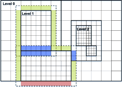
Figure 1.— Two-dimensional example of a three-level AMR hierarchy, with the base level ($\ell=0$) covering the entire computational domain. Solid lines are representative of the level resolution. Dashed lines contour the ghost zones of two patches of level $\ell=1$. Colors indicate different filling methods: physical outer boundaries (red), boundaries filled by exchanging values with adjacent patches on the same level (blue), boundaries filled by interpolating from the next coarser level (yellow).

The support for Adaptive Mesh Refinement (AMR) calculations in PLUTO is provided by the CHOMBO library. CHOMBO is a software package aimed at providing a distributed infrastructure for serial and parallel calculations over block-structured, adaptively refined grids in multiple dimensions. It is written in a combination of C++ and Fortran77 with MPI and is developed and distributed by the Applied Numerical Algorithms Group of Lawrence Berkeley National Laboratory (https://seesar.lbl.gov/anag/chombo/).

In the block-structured AMR approach, once the solution has been computed over a rectangular grid which discretizes the entire computational domain, it is possible to identify the cells which require additional resolution and cover them with a set of rectangular grids (also referred to as blocks or patches), characterized by a finer mesh spacing. CHOMBO follows the Berger & Rigoutsos (1995) strategy to determine the most efficient patch layout to cover the cells that have been tagged for refinement. This process can be repeated recursively to define the solution over a hierarchy of $\ell=0,\dots,\ell_{\mathrm{max}}$ levels of refinement whose spatial resolutions satisfy the relation $\Delta x_{d}^{\ell}=r^{\ell}\;\Delta x_{d}^{\ell+1}$, where the integer $r^{\ell}$ is the refinement ratio between level $\ell$ and level $\ell+1$. A level of refinement is composed by a union of rectangular grids which has to be: disjointed, i.e. two blocks of the same level can be adjacent without overlapping; properly nested, i.e. a cell of level $\ell$ cannot be only partially covered by cells of level $\ell+1$ and cells of level $\ell+1$ must be separated from cells of level $\ell-1$ at least by a row of cells of level $\ell$. A simple example of a bidimensional adaptive grid distributed over a hierarchy of three levels of refinement is depicted in Fig. 1.

Following the notation of Pember et al. (1996), a global mapping is employed on all levels: in three dimensions, cells on level $L$ are identified with global indexes $i,j,k$ ($0\leq i<N_{1}^{\ell}$, $0\leq j<N_{2}^{\ell}$, $0\leq k<N_{3}^{\ell}$, with $N_{1,2,3}^{\ell}$ being the equivalent global resolution of level $\ell$ in the three directions). Correspondingly, the cell $i,j,k$ of level $\ell$ is covered by $(r^{\ell})^{3}$ cells of level $\ell+1$ identified by global indexes $l,m,n$ satisfying the conditions $r^{\ell}i\leq l\leq r^{\ell}(i+1)-1$, $r^{\ell}j\leq m\leq r^{\ell}(j+1)-1$, $r^{\ell}k\leq n\leq r^{\ell}(k+1)-1$. Taking direction 1 as an example, the expressions $x_{1,-}^{\ell}=i\Delta x_{1}^{\ell}$, $x_{1}^{\ell}=(i+1/2)\Delta x_{1}^{\ell}$, $x_{1,+}^{\ell}=(i+1)\Delta x_{1}^{\ell}$, define the physical coordinates of the left edge, center and right edge of a cell respectively.

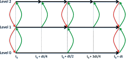
Figure 2.— Schematic representation of the time evolution of an AMR hierarchy composed by three levels with a refinement ratio $r=2$. The length of the horizontal black arrows is proportional to the timestep size $\Delta t^{\ell}$. Curved vertical arrows indicate interlevel communications. Red arrows represent fine-to-coarse communications between synchronized adjacent levels, including conservative averaging (Eq. 47) and refluxing (Eq. 48, 49). Green arrows represent coarse-to-fine communications, including the conservative interpolation (Eq. 45) needed to fill ghost zones and to define the solution on newly generated cells of the finer level.

If the adaptive grid is employed to evolve time-dependent hyperbolic partial differential equations, the CFL stability condition allows to apply refinement in time as well as in space, as first proposed by Berger & Oliger (1984) and further developed in Berger & Colella (1989). In fact, each level $\ell$ advances in time with a time-step $\Delta t^{\ell}=\Delta t^{\ell-1}/r^{\ell-1}$ which is $r^{\ell-1}$ times smaller than the time-step of the next coarser level $\ell-1$. Starting the integration at the same instant, two adjacent levels synchronize every $r^{\ell}$ timesteps, as schematically illustrated in Fig. 2 for a refinement ratio $r^{\ell}=2$. Even though in the following discussion we will assume that level $\ell+1$ completes $r^{\ell}$ timesteps to synchronize with level $\ell$, CHOMBO allows the finer level $\ell+1$ to advance with smaller substeps if the stability condition requires it. Anyway, the additional substeps must guarantee that levels $\ell$ and $\ell+1$ are synchronized again at time $t^{\ell}+\Delta t^{\ell}$.

The time evolution of single patches is handled by PLUTO , as illustrated in Section 3. Before starting the time evolution, the ghost cells surrounding the patches must be filled according to one of these three possibilities: (1) assigning “physical” boundary conditions to the ghost cells which lie outside the computational domain (e.g. the red area in Fig. 1); (2) exchanging boundary conditions with the adjacent patches of the same level (e.g. the blue area in Fig. 1); (3) interpolating values from the parent coarser level for ghost cells which cover cells of a coarser patch (e.g. the yellow area in Fig. 1).

Table 1Systems of coordinates adopted in PLUTO-CHOMBO

	Cartesian	Cylindrical
$x_{1}$	$x$	$r$
$x_{2}$	$y$	$z$
$x_{3}$	$z$	/
$V_{1}$	$x$	$r^{2}/2$
$V_{2}$	$y$	$z$
$V_{3}$	$z$	/
$A_{1,+}$	$\Delta y\Delta z$	$r_{+}\Delta z$
$A_{2,+}$	$\Delta z\Delta x$	$r\Delta r$
$A_{3,+}$	$\Delta x\Delta y$	/
${\cal V}$	$\Delta x\Delta y\Delta z$	$r\Delta r\Delta z$

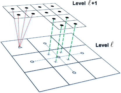
Figure 3.— Illustrative bidimensional example of prolongation and restriction operations between two levels with a refinement ratio $r^{\ell}$ = 2. Cells on level $\ell+1$ can be filled by linearly interpolating the coarse values on level $\ell$ (empty circles) at cross-marked points (prolongation, green dashed lines, Eq. 45). Cells on level $\ell$ can be filled by averaging down values from level $\ell+1$ in a conservative way (restriction, red dotted lines, Eq. 47).

Figure 4.— Pseudocode for the recursive level integration in the block structured AMR.

As schematically illustrated in Fig. 3 in two dimensions, the coarse-to-fine prolongation needed in case (3) (green dashed lines) is based on a piecewise linear interpolation at points marked by crosses using the linear slopes computed from the surrounding coarse cells. In three dimensions the interpolant has the general form:

$$\mathbf{U}_{l,m,n}^{\ell+1}=\mathbf{U}_{i,j,k}^{\ell}+\sum_{d=1}^{3}\frac{{\cal V}_{d}^{\ell+1}-{\cal V}_{d}^{\ell}}{{\cal V}_{d,+}^{\ell}-{\cal V}_{d,-}^{\ell}}\Delta_{d}\mathbf{U}_{i,j,k}^{\ell}\;,$$ (45)

where ${\cal V}_{d}^{\ell}$ is the volume coordinate of cell centers of level $\ell$ in direction $d$ and ${\cal V}_{d,\pm}^{\ell}$ is its value on the right and left faces of the cell respectively (see Table 1 for definitions). The linear slopes $\Delta_{d}\mathbf{U}_{i,j,k}^{\ell}$ are calculated as central differences, except for cells touching the domain boundary, where one-sided differences are employed. The monotonized-central limiter (Eq 34) is applied to the linear slopes so that no new local extrema are introduced.

Notice that, since two contiguous levels are not always synchronized (see Fig. 2), coarse values at an intermediate time are needed to prolong the solution from a coarse level to the ghost zones of a finer level. Coarse values of level $\ell$ are therefore linearly interpolated between time $t^{\ell}$ and time $t^{\ell}+\Delta t^{\ell}$ and the piecewise linear interpolant Eq. (45) is applied to the coarse solution

$$\mathbf{U}_{i,j,k}^{\ell*}=(1-\alpha)\mathbf{U}^{\ell}_{i,j,k}(t^{\ell})+\alpha\mathbf{U}^{\ell}_{i,j,k}(t^{\ell}+\Delta t^{\ell})\;,$$ (46)

where $\alpha=(t^{\ell+1}-t^{\ell})/\Delta t^{\ell}$. This requires that, everytime level $\ell$ and level $\ell+1$ are synchronized, a timestep on level $\ell$ must be completed before starting the time integration of level $\ell+1$. Therefore, the time evolution of the entire level hierarchy is performed recursively from level $\ell=0$ up to $\ell=\ell_{\max}$, as schematically illustrated by the pseudo-code in Fig. 4.

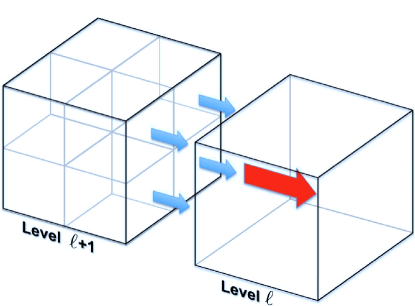
Figure 5.— Schematic visualization of the refluxing operation needed at fine-coarse interfaces to preserve the conservative properties of the solution. One cell on the coarser level $\ell$ and the cells of level $\ell+1$ adjacent on one side are represented, assuming a refinement ratio $r^{\ell}=2$. Whenever level $\ell$ and $\ell+1$ are synchronized, the coarse flux (red arrow) must be replaced by the spatial and temporal average of the finer fluxes crossing the fine-coarse interface (blue arrows, Eq. 48) and the solution must be corrected accordingly (Eq. 49).

When two adjacent levels are synchronized, some corrections to the solutions are performed to enforce the conservation condition on the entire level hierarchy. To maintain consistency between levels, the solution on the finer level $\ell+1$ is restricted to the lower level $\ell$ by averaging down the finer solution in a conservative way (red dotted lines in Fig. 3)

$$\mathbf{U}_{i,j,k}^{\ell}=\sum_{l=r^{\ell}i}^{r^{\ell}(i+1)-1}\sum_{m=r^{\ell}j}^{r^{\ell}(j+1)-1}\sum_{n=r^{\ell}k}^{r^{\ell}(k+1)-1}\frac{{\cal V}_{l,m,n}^{\ell+1}\mathbf{U}_{l,m,n}^{\ell+1}}{{\cal V}_{i,j,k}^{\ell}}\;,$$ (47)

where ${\cal V}_{i,j,k}^{\ell}$ is the volume of cell $i,j,k$ of level $\ell$.

Moreover, the flux through an edge which is shared between a cell of level $\ell$ and $(r^{\ell})^{2}$ cells of level $\ell+1$ must be corrected to maintain the conservative form of the equations. For example if the cell $i,j,k$ on level $\ell$ shares its left boundary with $(r^{\ell})^{2}$ cells of level $\ell+1$ (see Fig. 5), the flux calculated during the coarse integration must be replaced with the average in time and space of the fluxes crossing the $(r^{\ell})^{2}$ faces of the finer level cells. In this particular example, the flux correction is defined as:

$$\delta\mathbf{F}_{d}^{\ell}=-A_{d,-}^{\ell}\mathbf{F}_{d,-}^{\ell}+\frac{1}{r^{\ell}}\sum_{q=1}^{r^{\ell}}\sum_{m=r^{\ell}j}^{r^{\ell}(j+1)-1}\sum_{n=r^{\ell}k}^{r^{\ell}(k+1)-1}A_{d,+}^{\ell+1}\mathbf{F}_{d,m,n,+}^{\ell+1,q}\;,$$ (48)

where the index $q$ sums over the timsteps of level $\ell+1$, while $m$ and $n$ are the indexes transverse to direction $d$. The flux correction is added to the solution on level $\ell$ after the time integration of level $\ell$ and $\ell+1$ has been completed:

$$\mathbf{U}_{i,j,k}^{\ell}=\mathbf{U}_{i,j,k}^{\ell}+\Delta t^{\ell}\frac{\delta\mathbf{F}_{d}^{\ell}}{{\cal V}_{i,j,k}^{\ell}}\;.$$ (49)

Finally, when levels from $\ell$ up to $\ell_{\mathrm{max}}$ are synchronized, it is possible to tag the cells which need refinement and generate a new hierarchy of grids on levels from $\ell+1$ up to $\ell_{\mathrm{max}}$ which covers the tags at each level. Whenever new cells are created on level $\ell+1$ it is possible to fill them interpolating from level $\ell$ according to Eq. (45). It is important to notice that this interpolant preserves the conservative properties of the solution.

4.1. Refinement Criteria

In PLUTO-CHOMBO zones are tagged for refinement whenever a prescribed function $\chi(\mathbf{U})$ of the conserved variables and of its derivatives exceeds a prescribed threshold, i.e., $\chi(\mathbf{U})>\chi_{r}$. Generally speaking, the refinement criterion may be problem-dependent thus requiring the user to provide an appropriate definition of $\chi(\mathbf{U})$. The default choice adopts a criterion based on the second derivative error norm (Löhner, 1987), where

$$\chi(\mathbf{U})=\sqrt{\frac{\sum_{d}|\Delta_{d,+\frac{1}{2}}\sigma-\Delta_{d,-\frac{1}{2}}\sigma|^{2}}{\sum_{d}\left(|\Delta_{d,+\frac{1}{2}}\sigma|+|\Delta_{d,-\frac{1}{2}}\sigma|+\epsilon\sigma_{d,{\rm ref}}\right)^{2}}}$$ (50)

where $\sigma\equiv\sigma(\mathbf{U})$ is a function of the conserved variables, $\Delta_{d,\pm\frac{1}{2}}\sigma$ are the undivided forward and backward differences in the direction $d$, e.g., $\Delta_{x,\pm\frac{1}{2}}\sigma=\pm(\sigma_{i\pm 1}-\sigma_{i})$. The last term appearing in the denominator, $\sigma_{d,{\rm ref}}$, prevents regions of small ripples from being refined (Fryxell et al., 2000) and it is defined by

$$\sigma_{x,{\rm ref}}=|\sigma_{i+1}|+2|\sigma_{i}|+|\sigma_{i-1}|$$ (51)

Similar expressions hold when $d=y$ or $d=z$. In the computations reported in this paper we use $\epsilon=0.01$ as the default value.

4.2. Time Step Limitation of Point-Local Source Terms

In the usual AMR strategy, grids belonging to level $\ell$ are advanced in time by a sequence of steps with typical size

$$\Delta t^{\ell,n+1}=\frac{\Delta t^{0}_{\min}}{(2)^{\ell}}\,,$$ (52)

where we assume, for simplicity, a grid jump of 2. Here $\Delta t^{0}_{\min}$ is chosen by collecting and re-scaling to the base grid the time steps from all levels available from the previous integration step:

$$\Delta t^{0}_{\min}=\min_{0\leq\ell\leq\ell_{\max}}\left[(2)^{\ell}\Delta t^{\ell,n}\right]\,,$$ (53)

where $\Delta t^{\ell,n}$ is computed using (24). However, this procedure may become inefficient in presence of source terms whose time scale does not depend on the grid size. As an illustrative example, consider a strong radiative shock propagating through a static cold medium. In the optically thin limit, radiative losses are assumed to be local functions of the state vector, but they do not involve spatial derivatives. If the fastest time scale in the problem is dictated by the cooling process, the time step should then become approximately the same on all levels, $\Delta t\approx\Delta t^{\ell}_{\rm rad}\approx\Delta t^{0}_{\rm rad}$, regardless of the mesh size. However from the previous equations, one can see that finer levels with $\ell>0$ will advance with a time step $(2)^{\ell}$ smaller than required by the single grid estimate. Eq. (52) is nevertheless essential for proper synchronization between nested levels.

Simple considerations show that this deficiency may be cured by treating split and leaf cells differently. Split zones in a given level $\ell$ are, in fact, overwritten during the projection step using the more accurate solution computed on children cells belonging to level $\ell+1$. Thus, accurate integration of the source term is not important for these cells and could even be skipped. From these considerations, one may as well evaluate the source term-related time step on leaf cells only, where the accuracy and stability of the computed solution is essential. This trick should speed up the computations by a factor of approximately $(2)^{\ell}$, thus allowing to take full advantage of the refinement offered by the AMR algorithm without the time step restriction. Besides, this should not alter nor degrade the solution computed during this single hierarchical integration step as long as the projection step precedes the regrid process.

The proposed modification is expected to be particularly efficient in those problems where radiative losses are stronger in proximity of steep gradients.

4.3. Parallelization and load balancing

Both PLUTO and PLUTO-CHOMBO support calculations in parallel computing environments through the Message Passing Interface (MPI). Since the time evolution of the AMR hierarchy is performed recursively, from lower to upper levels, each level of refinement is parallelized independently by distributing its boxes to the set of processors. The computation on a single box has no internal parallelization. Boxes are assigned to processors by balancing the computational load on each processor. Currently, the workload of a single box is estimated by the number of grid points of the box, considering that the integration requires approximately the same amount of flops per grid point. This is not strictly true in some specific case, e.g in the presence of optically thin radiative losses, and a strategy to improve the load balance in such situations is currently under development. On the basis of the box workloads, CHOMBO’s load balancer uses the Kernighan-Lin algorithm for solving knapsack problems.

CHOMBO weak scaling performance has been thoroughly benchmarked: defining the initial setup by spatially replicating a 3D hydrodynamical problem proportionally to the number of CPUs employed, the execution time stays constant with excellent approximation (see Van Straalen, 2009, for more details).

To test the parallel performance of PLUTO-CHOMBO in real applications, we performed a number of strong scaling tests by computing the execution time as a function of the number of processors for a given setup. While this is a usual benchmark for static grid calculations, in the case of AMR computations this diagnostic is strongly problem-dependent and difficult to interpret.

In order to find some practical rule to improve the scaling of AMR calculations, we investigated the dependency of the parallel performance on some parameters characterizing the adaptive grid structure: the maximum box size allowed and the number of levels of refinement employed using different refinement ratios. As a general rule, the parallel performance deteriorates when the number of blocks per level becomes comparable to the number of processors or, alternatively, when the ideal workload per processor (i.e. the number of grid cells of a level divided by the number of CPUs) becomes comparable to the maximum box size. As we will show, decreasing the maximum possible block size can sensibly increase the number of boxes of a level and therefore improves the parallel performance. On the other hand, using less refinement levels with larger refinement ratios to achieve the same maximum resolution can lower the execution time, reducing the parallel communication volume and avoiding the integration of intermediate levels.

In Section 5 and 6 we will present several parallel scaling tests and their dependence on the aforementioned grid parameters.

5. MHD Tests

In this section we consider a suite of test problems specifically designed to assess the performance of PLUTO-CHOMBO for classical MHD flows. The selection includes one, two and three-dimensional standard numerical benchmarks already presented elsewhere in the literature as well as applications of astrophysical relevance. The single-patch integrator adopts the characteristic tracing step described in section 3.2 with either PPM, WENO or linear interpolations carried out in characteristic variables.

5.1. Shock tube problems

The shock tube test problem is a common benchmark for an accurate description of both continuous and discontinuous flow features. In the following we consider one and three dimensional configurations of standard shock tubes proposed by Torrilhon (2003) and Ryu & Jones (1995).

5.1.1 One-Dimensional Shock tube

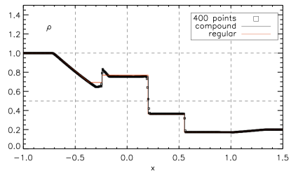
Figure 6.— Density profiles for the 1D shock tube problem at $t=0.4$ with $\alpha=\pi$. Solid lines correspond to admissible analytic solutions with (black) and without (red) a compound wave. The numerical solution (symbols) is obtained with 400 grid points.

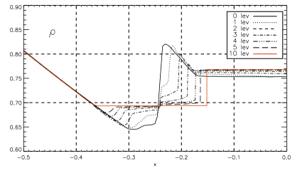
Figure 7.— Density profiles for the 1D shock tube problem at $t=0.4$ at the vicinity of the compound wave locus, with $\alpha=3$. The AMR levels vary from $0$ to $10$ as reported in the legend, exploring cases of equivalent resolution of $512$ (solid), $1024$ (dot), $2048$ (dash), $4096$ (dot-dash), $8192$ ($3$ dot-dash), $16,384$ (long dash) and $1,048,576$ (solid red) points. At high resolution the solution converges to the regular one. This figure is analogous to fig. 3 of Fromang et al. (2006).

Following Torrilhon (2003) we address the capability of the AMR scheme to handle and refine discontinuous features as well as to correctly resolve the non uniqueness issue of MHD Riemann problems in finite volume schemes (Torrilhon, 2003; Torrilhon & Balsara, 2004 and references therein). Left and right states are given by

$$\left\{\begin{array}[]{lclr}\mathbf{V}_{L}&=&\displaystyle\left(1,0,0,0,1,1,0,1\right)^{T}&\mathrm{for}\quad x_{1}<0\,,\\ \vskip 6.0pt plus 2.0pt minus 2.0pt\cr\mathbf{V}_{R}&=&\displaystyle\left(0.2,0,0,0,1,\cos(\alpha),\sin(\alpha),0.2\right)^{T}&\mathrm{for}\quad x_{1}>0\,,\end{array}\right.$$ (54)

where $\mathbf{V}=\left(\rho,v_{x},v_{y},v_{z},B_{x},B_{y},B_{z},p\right)$ is the vector of primitive variables and $\Gamma=2$. As discussed by Torrilhon (2003), for a wide range of initial conditions MHD Riemann problems have unique solutions, consisting of Lax shocks, contact discontinuities or usual rarefaction waves. Nevertheless, there exist certain sets of initial values that can result in non unique solutions. When this occurs, along with the regular solution arises one that allows for irregular MHD waves, for example a compound wave. A special case where the latter appears is when the initial transverse velocity components are zero and the magnetic field vectors are anti-parallel. Such a case was noted by Brio & Wu (1988) and can be reproduced by simply choosing $\alpha=\pi$ in our initial condition.

A one dimensional non unique solution is calculated using a static grid with $400$ zones, $x\in[-1,1.5]$. Left and right boundaries are set to outflow and the evolution stops at time $t=0.4$, before the fast waves reach the borders. The resulting density profile is shown in Fig. (6). The solid lines denote the two admissible exact solutions: the regular (red) and the one containing a compound wave (black), the latter situated at $x\,\sim\,-0.24$. It is clear that the solution obtained with the Godunov-type code is the one with the compound wave (symbols).

The crucial problematic of this test occurs when $\alpha$ is close to but not exactly equal to $\pi$. Torrilhon (2003) has proven that regardless of scheme, the numerical solution will erroneously tend to converge to an “irregular” one similar to $\alpha=\pi$ (pseudo-convergence), even if the initial conditions should have a unique, regular solution. This pathology can be cured either with high order schemes (Torrilhon & Balsara, 2004) or with a dramatic increase in resolution on the region of interest, proving AMR to be quite a useful tool. To demonstrate this we choose $\alpha=3$ for the field’s twist.

Table 2CPU running time for the one-dimensional MHD shock-tube using both static and AMR computations.

Static Run		AMR Run			Gain
$N_{x}$	Time (s)	Level	Ref ratio	Time (s)
512	0.5	0	2	0.5	1
1024	1.9	1	2	1.1	1.7
2048	7.5	2	2	2.3	3.3
4096	31.6	3	2	4.5	7.0
8192	138.0	4	2	8.7	15.9
16384	546.1	5	2	16.9	32.3
1048576	2.237 $\cdot 10^{6}$†	10	2 (4)	1131.1	1977.8

Note. — The first and second columns give the number of points $N_{x}$ and corresponding CPU for the static grid run (no AMR). The third, fourth and fifth columns give, respectively, the number of levels, the refinement ratio and CPU time for the AMR run at the equivalent resolution. The last row refers to the solid red line of Fig. 7, where a jump ratio of four was introduced between levels $6$ and $7$ to reach an equivalent of $\sim 10^{6}$ grid points. The last column shows the corresponding gain factor calculated as the ratio between static and AMR execution time.

Starting from a coarse grid of $512$ computational zones, we vary the number of refinement levels, with a consecutive jump ratio of two. The $10$ level run (solid red line) incorporates also a single jump ratio of four between the sixth and seventh refinement levels, reaching a maximum equivalent resolution of $1,048,576$ zones (see Fig. 7). The refinement criterion is set upon the variable $\sigma=(B_{x}^{2}+B_{y}^{2}+B_{z}^{2})/\rho$ using Eq. (50) with a threshold $\chi_{r}=0.03$, whereas integration is performed using PPM with a Roe Riemann solver and a Courant number $C_{a}=0.9$. As resolution increases the compound wave disentangles and the solution converges to the expected regular form (Torrilhon, 2003; Fromang et al., 2006). In Table 2 we compare the CPU running time of the AMR runs versus static uniform grid computations at the same effective resolution. With 5 and 10 levels of refinement (effective resolutions 16,384 and 1,048,576 zones, respectively) the AMR approach is $\sim 32$ and $\sim 1978$ times faster than the uniform mesh computation, respectively.

5.1.2 Three-Dimensional Shock tube

Figure 8.— Primitive variable profiles for the 3D shock tube problem at $t=0.02\cos\alpha\cos\gamma$, along the $x$ direction. Density and thermal pressure are plotted in the top panels while vector field components normal (“1”) and transverse (“2” and “3”) to the initial surface of discontinuity are shown in the middle and bottom panels. We show a smaller portion of the domain, $x\in[-0.25,0.55]$, in order to emphasize the change of resolution by symbol density.

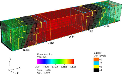
Figure 9.— Closeup of the top-hat feature in the density profile for the 3D shock tube problem, along with AMR level structure and the mesh. Different colors are used to distinguish grid levels.

The second Riemann problem was proposed by Ryu & Jones (1995) and later considered also by Tóth (2000), Balsara & Shu (2000), Gardiner & Stone (2008), Mignone & Tzeferacos (2010), Mignone et al. (2010). An initial discontinuity is described in terms of primitive variables as

$$\left\{\begin{array}[]{lclr}\mathbf{V}_{L}&=&\displaystyle\left(1.08,1.2,0.01,0.5,\frac{2}{\sqrt{4\pi}},\frac{3.6}{\sqrt{4\pi}}\frac{2}{\sqrt{4\pi}},0.95\right)^{T}\\ \vskip 6.0pt plus 2.0pt minus 2.0pt\cr&&\quad\quad\quad\quad\quad\quad\quad\quad\quad\quad\quad\quad\mathrm{for}\quad x_{1}<0\\ \vskip 6.0pt plus 2.0pt minus 2.0pt\cr\mathbf{V}_{R}&=&\displaystyle\left(1,0,0,0,\frac{2}{\sqrt{4\pi}},\frac{4}{\sqrt{4\pi}},\frac{2}{\sqrt{4\pi}},1\right)^{T}\\ \vskip 6.0pt plus 2.0pt minus 2.0pt\cr&&\quad\quad\quad\quad\quad\quad\quad\quad\quad\quad\quad\quad\mathrm{for}\quad x_{1}>0\end{array}\right.$$ (55)

where $\mathbf{V}=\left(\rho,v_{1},v_{2},v_{3},B_{1},B_{2},B_{3},p\right)$ is the vector of primitive variables. The subscript “1” gives the direction perpendicular to the initial surface of discontinuity whereas “2” and “3” correspond to the transverse directions. We first obtain a one-dimensional solution on the domain $x\in[-0.75,0.75]$ using 6144 grid points, stopping the computations at $t=0.2$.

In order to test the ability of the AMR scheme to maintain the translational invariance and properly refine the flow discontinuities, the shock tube is rotated in a three dimensional Cartesian domain. The coarse level of the computational domain consists of $[384\times 4\times 4]$ zones and spans $[-0.75,0.75]$ in the $x$ direction while $y,z\,\in[0,0.015625]$. The rotation angles, $\gamma$ around the $y$ axis and $\alpha$ around the $z$ axis, are chosen so that the planar symmetry is satisfied by an integer shift of cells $(n_{x},n_{y},n_{z})$. The rotation matrix can be found in Mignone et al. (2010). By choosing $\tan\alpha=-r_{1}/r_{2}$ and $\tan\beta=\tan\gamma/\cos\alpha=r_{1}/r_{3}$, one can show (Gardiner & Stone, 2008) that the three integer shifts $n_{x},n_{y},n_{z}$ must obey

$$n_{x}-n_{y}\frac{r_{1}}{r_{2}}+n_{z}\frac{r_{1}}{r_{3}}=0\,,$$ (56)

where cubed cells have been assumed and $(r_{1},r_{2},r_{3})=(1,2,4)$ will be used. Computations stop at $t=0.2\cos\alpha\cos\gamma$, once again before the fast waves reach the boundaries. We employ 4 refinement levels with consecutive jumps of two, corresponding to an equivalent resolution of $6144\times 64\times 64$ zones. The refinement criterion is based on the normalized second derivative of $\chi=(|B_{x}|+|B_{y}|)\rho$ with a threshold value $\chi_{r}=0.1$. Integration is done with PPM reconstruction, a Roe Riemann solver and a Courant number of $C_{a}=0.4$.

The primitive variable profiles (symbols) are displayed in Fig. 8 along the $x$ direction, together with the one dimensional reference solution in the $x\in[-0.25,0.55]$ region. In agreement with the solution of Ryu & Jones (1995), the wave pattern produced consists of a contact discontinuity that separates two fast shocks, two slow shocks and a pair of rotational discontinuities. A three dimensional closeup of the top-hat feature in the density profile is shown in Fig. 9, along with AMR levels and mesh. The discontinuities are captured correctly, and the AMR grid structure respects the plane symmetry. Our results favorably compare with those of Gardiner & Stone (2008); Mignone & Tzeferacos (2010); Mignone et al. (2010) and previous similar 2D configurations.

The AMR computation took approximately $3\,{\rm hours}$ and $53$ minutes on two $2.26\,\textrm{GHz}$ Quad-core Intel Xeon processors ($8$ cores in total). For the sake of comparison, we repeated the same computation on a uniform mesh of $768\times 8\times 8$ zones ($1/8$ of the effective resolution) with the static grid version of PLUTO employing $\approx 79$ seconds. Thus, extrapolating from ideal scaling, the computational cost of the fixed grid calculation is expected to increase by a factor $2^{12}$ giving an overall gain of the AMR over the uniform grid approach of $\sim 23$.

5.2. Advection of a magnetic field loop

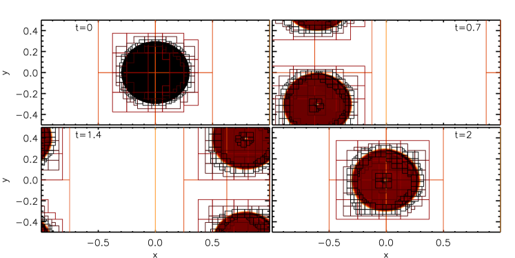
Figure 10.— Magnetic energy density for the 2D field loop problem at $t=0,\,0.7,\,1.4,\,2$. Overplotted are the refinement levels.

Figure 11.— Upper panel: Normalized magnetic energy for the field loop advection problem as a function of time. Lower panel: computational time as a function of equivalent resolution.

The next test problem considers the two dimensional advection of a magnetic field loop. This test, proposed by Gardiner & Stone (2005), aims to benchmark the scheme’s dissipative properties and the correct discretization balance of multi-dimensional terms through monitoring the preservation of the initial circular shape of the loop.

As in Gardiner & Stone (2005) and Fromang et al. (2006), we define the computational domain by $x\in[-1,1]$ and $y\in[-0.5,0.5]$ discretized on a coarse grid of $64\times 32$ grid cells. In the initial condition, both density and pressure are uniform and equal to $1$, while the velocity of the flow is given by $\mathbf{v}=V_{0}\cos\alpha\hat{\mathbf{e}}_{x}+V_{0}\sin\alpha\hat{\mathbf{e}}_{y}$ with $V_{0}=\sqrt{5}$, $\sin\alpha=1/\sqrt{5}$ and $\cos\alpha=2/\sqrt{5}$. The magnetic field is then defined through its magnetic vector potential as

$$A_{z}=\left\{\begin{array}[]{ll}A_{0}(R-r)&\textrm{if}\quad r\leq R\,,\\ \vskip 6.0pt plus 2.0pt minus 2.0pt\cr 0&\textrm{if}\quad r>R\,,\end{array}\right.$$ (57)

where $A_{0}=10^{-3}$, $R=0.3$, and $r=\sqrt{x^{2}+y^{2}}$. The simulation evolves until $t=2$, when the loop has thus performed two crossing through the periodic boundaries. The test is repeated with $2$, $3$ and $4$ levels of refinement (jump ratio of two), resulting to equivalent resolutions of $[256\times 128]$, $[512\times 256]$ and $[1024\times 512]$ respectively. Refinement is triggered whenever the second derivative error norm of $(B_{x}^{2}+B_{y}^{2})\times 10^{6}$, computed via Eq. (50), exceeds the threshold $\chi_{r}=0.1$. The integration is carried out utilizing WENO reconstruction and the Roe Riemann solver, with $C_{a}=0.4$.

The temporal evolution of magnetic energy density is seen in Fig. (10), with $4$ levels of refinement. As the field loop is transported inside the computational domain, the grid structure changes to follow the evolution and retain the initial circular form. An efficient way to quantitatively measure the diffusive properties of the scheme is to monitor the dissipation of the magnetic energy. In the top panel of Fig. (11) we plot the normalized mean magnetic energy as a function of time. By increasing the levels of refinement the dissipation of magnetic energy decreases, with $<{\bf B}^{2}>$ ranging from $\sim 94\%$ to $\sim 98\%$ of the initial value. In order to quantify the computational gain of the AMR scheme we repeat the simulations with a uniform grid resolved onto as many points as the equivalent resolution, without changing the employed numerical method. The speed-up is reported in the bottom panel of Fig. 11.

5.3. Resistive Reconnection

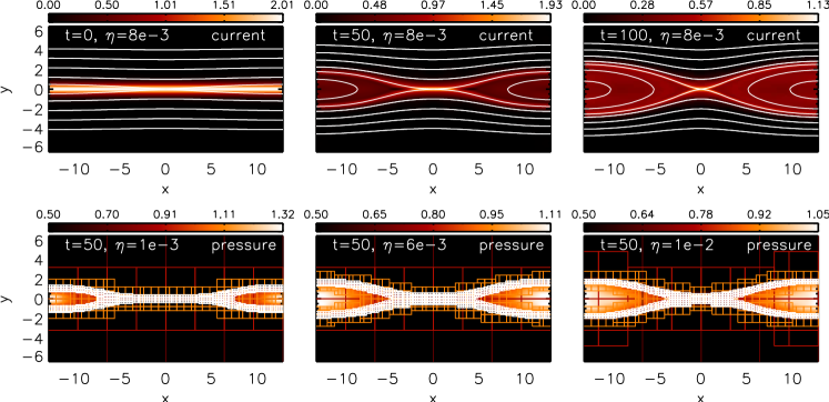
Figure 12.— Upper row: temporal evolution of the current density and magnetic field lines for the resistive reconnection problem, with $\eta=8\,10^{-3}$. Snapshots refer to $t=0,\,50,\,100$. Lower row: Pressure profiles for various values of resistivity $\eta$, along with the AMR level structure at $t=50$. The refinement strategy consists of $3$ levels with a jump ratio of $2:4:4$ (equivalent resolution of $2048\times 1024$ mesh points).

Figure 13.— Time average of $\delta/L$, analogous to the magnetic reconnection rate ${\cal E}$, as a function of resistivity. Symbols represent the actual data, whereas over-plotted (dashed line) is the Sweet-Parker scaling $\sim\sqrt{\eta}$, along with a best fit (solid line). The numerical results are in agreement with the theoretical scaling.

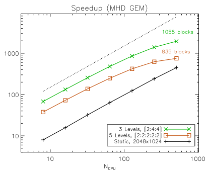
Figure 14.— Parallel speedup at $t=50$ as a function of the number of processors ($N_{\rm CPU}$) for the resistive reconnection problem. The different lines refer to the execution times obtained with 5 levels of refinement with consecutive jumps of 2 (red squares), 3 levels with jump ratios $2:4:4$ (green crosses) and a fixed uniform grid with $2048\times 1024$ zones (black plus signs). The dotted line gives the ideal scaling whereas the number of blocks on the finest level at the end of integration is reported above each curve.

Magnetic reconnection refers to the process of breaking and reconnection of magnetic field lines with opposite directions, accompanied with a conversion of magnetic energy into kinetic and thermal energy of the plasma. This is believed to be the basic mechanism behind energy release during solar flares. The first solution to the problem was given independently by Sweet (1958) and Parker (1957), treating it as a two dimensional boundary layer problem in the laminar limit.

According to the Sweet-Parker model, the magnetic field’s convective inflow is balanced by Ohmic diffusion. Along with the assumption of continuity, this yields a relation between reconnection and plasma parameters. If $L$ and $\delta$ are the boundary layer’s half length and width respectively, we can write the reconnection rate ${\cal E}$ as

$${\cal E}\equiv\frac{u_{\textrm{in}}}{u_{\textrm{out}}}\sim\frac{\delta}{L}\sim\frac{1}{\sqrt{S}}.$$ (58)

With $u_{\textrm{in}}$ and $u_{\textrm{out}}$ we denote the inflow and outflow speeds, into and out of the boundary layer, respectively. The Lundquist number for the boundary layer is defined as $S=u_{A}L/\eta$, with $u_{A}$ being the Alfvén velocity directly upstream of the layer, $\eta$ the magnetic resistivity and $L$ the layer’s half length. This dependency of the reconnection rate with the square root of magnetic resistivity is called the Sweet-Parker scaling and has been verified both numerically (Biskamp, 1986; Uzdensky & Kulsrud, 2000) and experimentally (Ji et al., 1998).

Following the guidelines of the GEM Magnetic Reconnection Challenge (Birn et al., 2001), the computational domain is a two dimensional Cartesian box, with $x\in[-L_{x}/2,L_{x}/2]$ and $y\in[-L_{y}/2,L_{y}/2]$ where we choose $L_{x}\,=\,25.6$ and $L_{y}\,=\,12.8$. The initial condition consists of a Harris current sheet: the magnetic field configuration is described by $B_{x}(y)=B_{0}\tanh(y/\lambda)$ whereas the flow’s density is $\rho=\rho_{0}\textrm{sech}^{2}(y/\lambda)+\rho_{\infty}$, where $\lambda=0.5$, $\rho_{0}=1$ and $\rho_{\infty}=0.2$. The flow’s thermal pressure is deduced assuming equilibrium with magnetic pressure, $P=B_{0}^{2}/2=0.5$. The initial magnetic field components are perturbed via

$$\begin{array}[]{ll}dB_{x}=-\Psi_{0}(\pi/L_{y})\sin(\pi y/L_{y})\cos(2\pi x/L_{x})\\ \vskip 6.0pt plus 2.0pt minus 2.0pt\cr dB_{y}=\Psi_{0}(2\pi/L_{x})\sin(2\pi x/L_{x})\cos(\pi y/L_{y}).\end{array}$$ (59)

where $\Psi_{0}=0.1$. The coarse grid consists of $[64\times 32]$ points and additional levels of refinement are triggered using the following criterion based on the current density:

$$\frac{\left|\Delta_{x}B_{y}-\Delta_{y}B_{x}\right|}{|\Delta_{x}B_{y}|+|\Delta_{y}B_{x}|+\sqrt{\rho}/\xi}>\frac{\chi_{\min}-\chi_{\max}}{1+(1-\xi)^{2}}+\chi_{\max}$$ (60)

where $\Delta_{x}B_{y}$ and $\Delta_{y}B_{x}$ are the undivided central differences of $B_{y}$ and $B_{x}$ in the $x$ and $y$ direction, respectively, and $\xi=\Delta x^{0}/\Delta x^{\ell}\geq 1$ is the ratio of grid spacings between the base ($0$) and current level ($l$). The threshold values $\chi_{\min}=0.2$ and $\chi_{\max}=0.37$ are chosen in such a way that refinement becomes increasingly harder for higher levels. We perform test cases using either $5$ levels of refinement with a consecutive jump ratio of two or $3$ levels with jump ratio $2:4:4$ reaching, in both cases, an equivalent resolution of $2048\times 1024$ mesh points. Boundaries are periodic in the $x$ direction, whereas perfectly conducting boundary walls are set at $y=\pm L_{y}/2$. We follow the computations until $t=100$ using PPM reconstruction with a Roe Riemann solver and a Courant number $C_{a}=0.8$. In Fig. 12 we display the temporal evolution of the current density for a case where the uniform resistivity is set to $\eta=8\cdot 10^{-3}$. A reconnection layer is created in the center of the domain, which predisposes resistive reconnection (Biskamp, 1986). In agreement with Reynolds et al. (2006) the maximum value of the current density decreases with time, (fig. 4 of that study). As seen in the first two panels ($t=0,\,50$), the refinement criterion is adequate to capture correctly both the boundary layer and the borders of the magnetic island structure. In the rightmost panel ($t=100$) we also draw sample magnetic field lines to better visualize the reconnection region.

In order to compare our numerical results with theory, we repeated the computation varying the value of the magnetic resistivity $\eta$. For small values of resistivity (large Lundquist numbers $S$), the boundary layer is elongated and presents large aspect ratios $A\equiv L/\delta$. Biskamp (1986) reports that for $A$ beyond the critical value of $A_{\textrm{crit}}\simeq 100$ the boundary layer is tearing unstable, limiting the resistivity range in which the Sweet-Parker reconnection model operates. Since in the Sun’s corona $S$ can reach values of $\sim 10^{14}>>S_{\max}$, secondary island formation must be taken into account (Cassak & Drake, 2009). In this context, ensuring that we respect Biskamp’s stability criterion, we calculate the temporal average of $\delta/L$, analogous to the reconnection rate ${\cal E}$, for various $\eta$ and reproduce the Sweet-Parker scaling (Fig. 13). The boundary layer’s half -width ($\delta$) and -length ($L$) are estimated from the e-folding distance of the peak of the electric current, while the AMR scheme allows us to economically resolve the layer’s thickness with enough grid points.

Parallel performance for this problem is shown in Fig. 14, where we plot the speedup $S=T_{1}/T_{N_{\rm CPU}}$ as a function of the number of processors $N_{\rm CPU}$ for the 3- and 5-level AMR computations as well as for fixed uniform grid runs carried out at the equivalent resolution of $2048\times 1024$ zones. Here $T_{1}$ is the same reference constant for all calculations and equal to the (inferred) running time of the single processor static mesh computation while $T_{N_{\rm CPU}}$ is the execution time measured with $N_{\rm CPU}$ processors. The scaling reveals an efficiency (defined as $S/N_{\rm CPU}$) larger than $0.8$ for less than $256$ processors with the 3- and 5-level computations being, respectively, $8$ to $9$ and $4$ to $5$ times faster than the fixed grid approach. The number of blocks on the finest level is maximum at the end of integration and is slightly larger for the 3-level run (1058 vs. 835). This result indicates that using fewer levels of refinement with larger grid ratios can be more efficient than introducing more levels with consecutive jumps of 2, most likely because of the reduced integration cost due to the missing intermediate levels and the decreased overhead associated with coarse-fine level communication and grid generation process. Efficiency quickly drops when the number of CPU tends to become, within a factor between $2$ and $3$, comparable to the number of blocks.

5.4. Current Sheet

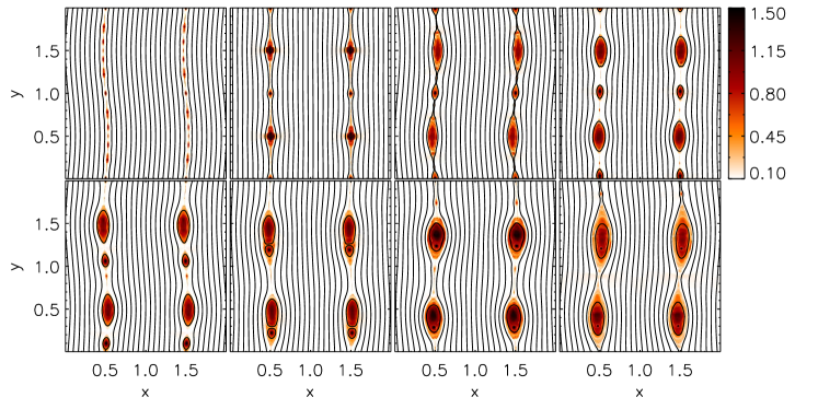
Figure 15.— Time evolution of the pressure profiles along with sample magnetic field lines, for the current sheet problem. Temporal snapshots refer to $t=0.5,\,1,\,1.5,\,2$ (upper four) and $t=2.5,\,3,\,3.5,\,4$ (lower four).

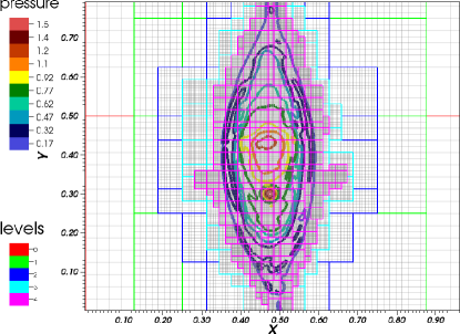
Figure 16.— Closeup of the bottom left island at $t=4$ for the current sheet problem. Pressure contours, along with the refinement levels and grid are shown.

The current sheet problem proposed by Gardiner & Stone (2005) and later considered by Fromang et al. (2006) in the AMR context is particularly sensitive to numerical diffusion. The test problem follows the evolution of two current sheets, initialized through a discontinuous magnetic field configuration. Driven solely by numerical resistivity, reconnection processes take place, making the resulting solution highly susceptible to grid resolution.

The initial condition is discretized onto a Cartesian two dimensional grid $x,\,y\in[0,2]$, with $64\times 64$ zones at the coarse level. The fluid has uniform density $\rho=1$ and thermal pressure $P=0.1$. Its bulk flow velocity ${\bf v}$ is set to zero, allowing only for a small perturbation in $v_{x}\,=\,v_{0}\,\sin(\pi\,y)$, where $v_{0}=0.1$. The initial magnetic field has only one non-vanishing component in the vertical direction,

$$B_{y}=\left\{\begin{array}[]{ll}-B_{0}&\textrm{if}\quad|x-1|\leq 0.5\,,\\ \vskip 6.0pt plus 2.0pt minus 2.0pt\cr\,\,\,\,B_{0}&\textrm{otherwise}\,,\end{array}\right.$$ (61)

where $B_{0}=1$, resulting in a magnetically dominated configuration. Boundaries are periodic and the integration terminates at $t=4$. We activate refinement whenever the maximum between the two error norms (given by Eq. 50) computed with the specific internal energy and the $y$ component of the magnetic field exceeds the threshold value $\chi_{r}=0.2$. In order to filter out noise between magnetic island we set $\epsilon=0.05$. We allow for $4$ levels of refinement and carry out integration with the Roe Riemann solver, the improved WENO reconstruction and a CFL number of $0.6$.

In Fig. 15 we show temporal snapshots of pressure profiles for $t=0.5,\,1.0,\,1.5,\,2,\,3.5$ and $4.0$, along with sample magnetic field lines. Since no resistivity has been specified, the elongated current sheets are prone to tearing instability as numerical resistivity is small with respect to Biskamp’s criterion (Biskamp, 1986). Secondary islands, “plasmoids”, promptly form and propagate parallel to the field in the $y$ direction. As reconnection occurs, the field is dissipated and its magnetic energy is transformed into thermal energy, driving Alfvén and compressional waves which further seed reconnection (Gardiner & Stone, 2005; Lee & Deane, 2009). Due to the dependency of numerical resistivity on the field topology, reconnection events are most probable at the nodal points of $v_{x}$. At the later stages of evolution, the plasmoids eventually merge in proximity of the anti-nodes of the transverse speed, forming four larger islands, in agreement with the results presented in Gardiner & Stone (2005). A closeup on the bottom left island is shown in Fig. 16, at the end of integration. The refinement criterion on the second derivative of thermal pressure, as suggested by Fromang et al. (2006), efficiently captures the island features of the solution.

5.5. Three-dimensional Rayleigh Taylor Instability

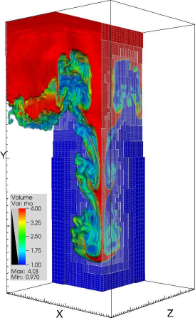
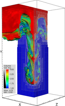
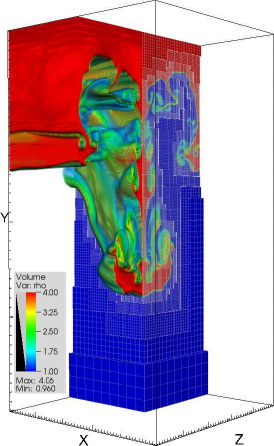
Figure 17.— Three-dimensional view of the Rayleigh-Taylor instability problem showing density at $t=3$ for the un-magnetized (left panel), weakly magnetized (middle panel) and strongly magnetized case (right panel) using $4$ levels of refinement. In each panel we also show a sliced boxed emphasizing the grid refinement ratios.

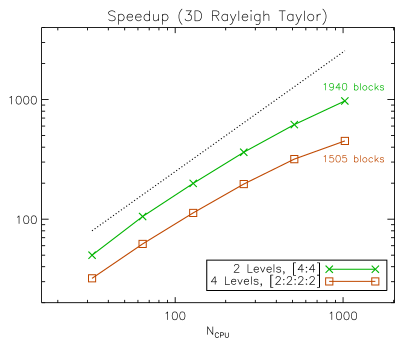
Figure 18.— Parallel speedup versus number of processors $N_{\rm CPU}$ for the 3D Rayleigh-Taylor problem computed with 2 (green crosses) and 4 (red squares) refinement levels between $t=2$ and $t=2.25$. The dotted line gives the ideal scaling. The number of blocks on the finest level at $t=2$ is printed above and below the corresponding curves.

In this example we consider the dynamical evolution of two fluids of different densities initially in hydrostatic equilibrium. If the lighter fluid is supporting the heavier fluid against gravity, the configuration is known to be subject to the Rayleigh-Taylor instability (RTI). Our computational domain is the box spanned by $x,z\in[-1/2,1/2]$, $y\in[-3/2,1/2]$ with gravity pointing in the negative $y$ direction, i.e. $\mathbf{g}=(0,-1,0)$. The two fluids are separated by an interface initially lying in the $xz$ plane at $y=0$, with the heavy fluid $\rho=\rho_{h}$ at $y>0$ and $\rho=\rho_{l}$ at $y<0$. In the current example we employ $\rho_{h}=4$, $\rho_{l}=1$ and specify the pressure from the hydrostatic equilibrium condition:

$$p(y)=\frac{100}{\gamma}-\rho y\,,$$ (62)

so that the sound crossing time in the light fluid is $0.1$. The seed for instability is set by perturbing the velocity field at the center of the interface:

$$v_{y}=-\frac{\exp\left[-(5r)^{2}\right]}{10\cosh(10y)^{2}}$$ (63)

where $r=\sqrt{x^{2}+z^{2}}$. We assume a constant magnetic field $\mathbf{B}=(B_{x},0,0)$ parallel to the interface and oriented in the $x$ direction with different field strengths, $B_{x}=0$ (hydro limit), $B_{x}=0.2B_{c}$ (moderate field) and $B_{x}=0.6B_{c}$ (strong field). Here $B_{c}=\sqrt{(\rho_{h}-\rho_{l})gL}$ is the critical field value above which instabilities are suppressed (Stone & Gardiner, 2007). We use the PPM method with the Roe Riemann solver and a Courant number $C_{a}=0.45$. The base grid has $16\times 32\times 16$ cells and we perform two sets of computations using i) $4$ refinement levels with a grid spacing ratio of $2$ and ii) $2$ refinement levels with a grid jump of $4$, in both cases achieving the same effective resolution ($256\times 512\times 256$). Refinement is triggered using the second derivative error norm of density and a threshold value $\chi_{\rm ref}=0.5$. Periodic boundary conditions are imposed at the $x$ and $z$ boundaries while fixed boundaries are set at $y=-3/2$ and $y=1/2$.

Results for the un-magnetized, weakly and strongly magnetized cases are shown at $t=3$ in Fig. 17. In all cases, we observe the development of a central mushroom-shaped finger. Secondary instabilities due to Kelvin-Helmholtz modes develop on the side and small-scale structures are gradually suppressed in the direction of the field as the strength is increased. Indeed, as pointed out by Stone & Gardiner (2007), the presence of a uniform magnetic field has the effects of reducing the growth rate of modes parallel to it although the interface still remains Rayleigh-Taylor unstable in the perpendicular direction due to interchange modes. As a net effect, the evolution becomes increasingly anisotropic as the field strengthens.

Parallel performance is plotted, for the moderate field case, in Fig. 18 where we measure the speedup factors of the 4- and 2- level computations versus the number of CPUs. Here the speedup is defined by $S=T_{1}/T_{N_{\rm CPU}}$ where $T_{1}$ is the inferred running time relative to the 4-level computation on a single-processor. The two-level case shows improved performance over the four-level calculation both in terms of CPU cost as well as parallel efficiency $S/N_{\rm CPU}$. Indeed the relative gain between the two cases approaches a factor of $2$ for an increasing number of CPUs. Likewise, the efficiency of the fewer level case remains above $\gtrsim 0.8$ up to $512$ processors and drops to $\sim 0.61$ (versus $\sim 0.44$ for the 4-level case) at the largest number of employed cores ($1024$) which is less than the number of blocks on the finest grid.

5.6. Two-dimensional Shock-Cloud Interaction

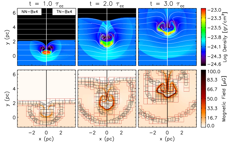
Figure 19.— Top panel: density maps (${\rm gr}/{\rm cm}^{3}$ in Log scale) for the shock-cloud interaction at $t=1,2,3$ for a magnetic field initially parallel to the shock interface (Bx4). Here the time unit is defined as the cloud crushing time and equal to $5,400\,{\rm yrs}$. Bottom panel: magnetic field strength (in units of $10^{-6}$ G) with the distribution of patches at levels $3$ and $4$ superimposed. The left and right half of each panel shows the results computed with the PPM method without (NN) and with (TN) thermal conduction, respectively. The resolution of the base grid is $32^{2}$ and $5$ levels of refinement are used.

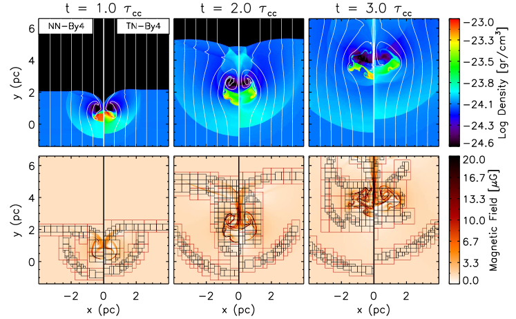
Figure 20.— Same as Fig. 19 but for a field initially pointing in the $y$ direction (that is, perpendicular to the shock front).

The shock-cloud interaction problem has been extensively studied and used as a standard benchmark for the validation of MHD schemes and inter-code comparisons (see Dai & Woodward, 1994; Balsara, 2001; Lee & Deane, 2009 and reference therein). In an astrophysical context, it adresses the fundamental issue of the complex morphology of supernova remnants as well as their interaction with the interstellar medium. Energy, mass and momentum exchange leading to cloud-crushing strongly depends on the orientation of the magnetic field and the resulting anisotropy of thermal conduction.

Following Orlando et al. (2008), we consider the two-dimensional Cartesian domain $x\in[-4,4]$, $y\in[-1.4\times 6.6]$ with the shock front propagating in the positive $y$ direction and initially located at $y=-1$. Ahead of the shock, for $y>-1$, the hydrogen number density $n_{1}$ has a radial distribution of the form:

$$n_{1}=n_{a}-\frac{n_{a}-n_{c}}{\cosh\left[\sigma(r/r_{\rm cl})^{\sigma}\right]}\,,\quad r=\sqrt{x^{2}+y^{2}}$$ (64)

where $n_{c}=1\,{\rm cm}^{-3}$ is the hydrogen number density at the cloud’s center, $n_{a}=0.1n_{c}$ is the ambient number density, $r_{\rm cl}=1\,{\rm pc}$ is the cloud’s radius ($\sigma=10$) and $r$ is the radial distance from the center of the cloud. The ambient medium has a uniform temperature $T_{a}=10^{4}\,{\rm K}$ in pressure equilibrium with the cloud, with a thermal pressure of $p_{1}=2k_{B}n_{a}T_{a}$ (we assume a fully ionized gas). Downstream of the shock, density and transverse components of the magnetic field are compressed by a factor of $n_{2}/n_{1}=(\Gamma+1)/(\Gamma-1)$ while pressure and normal velocity are given by

$$p_{2}=2n_{2}k_{B}T_{s}\,,\quad v_{y,2}=\sqrt{\frac{2}{\Gamma-1}\frac{2k_{B}T_{s}}{\mu m_{H}}}$$ (65)

where $\mu=1.26$ is the inverse of the hydrogen mass fraction and $T_{s}=4.7\cdot 10^{6}\,{\rm K}$ is the post-shock temperature. The normal component of the magnetic field ($B_{y}$) remains continuous through the shock front.

We perform two sets of simulations with a magnetic field strength of $|\mathbf{B}|=1.31\;\mu{\rm G}$, initially parallel (case Bx4) or perpendicular (case By4) to the shock front. Adopting the same notations as Orlando et al. (2008), we solve in each case the MHD equations with (TN) and without (NN) thermal conduction effects for a total of 4 cases. Thermal conductivity coefficients along and across the magnetic field lines (see Eq. 6) are given, in c.g.s units, by

$$k_{\parallel}=\displaystyle 9.2\cdot 10^{-7}T^{5/2}\,,\quad k_{\perp}=\displaystyle 5.4\cdot 10^{-16}\frac{n_{H}^{2}}{\sqrt{T}\mathbf{B}^{2}}\,.$$ (66)

The resolution of the base grid is set to $32^{3}$ points and $5$ levels of refinement are employed, yielding an equivalent resolution of $1024\times 1024$. Upwind characteristic tracing (Section 3.2) together with PPM reconstruction (Eq. 33) and the HLLD Riemann solver are chosen to advance the equations in time. Open boundary conditions are applied on all sides, except at the lower $y$ boundary where we keep constant inflow values. The CFL number is $C_{a}=0.8$. Refinement is triggered upon density with a threshold $\chi_{\rm ref}=0.15$.

In Fig. 19 and 20 we show the cloud evolution for the four different cases at three different times $t=1,2,3$ (in units of the cloud crushing time $\tau_{cc}=5.4\cdot 10^{3}\,{\rm yrs}$). Our results are in excellent agreement with those of Orlando et al. (2008) confirming the efficiency of thermal conduction in suppressing the development of hydrodynamic instabilities at the cloud borders. The topology of the magnetic field can be quite effective in reducing the efficiency of thermal conduction. For a field parallel to the shock front (TN-Bx4), the cloud’s expansion and evaporation are strongly limited by the confining effect of the enveloping magnetic field. In the case of a perpendicular field (TN-By4), on the contrary, thermal exchange between the cloud and its surroundings becomes more efficient in the upwind direction of the cloud and promotes the gradual heating of the core and the consequent evaporation in a few dynamical timescales. In this case, heat conduction is strongly suppressed laterally by the presence of a predominantly vertical magnetic field.

5.7. Radiative Shocks in Stellar Jets

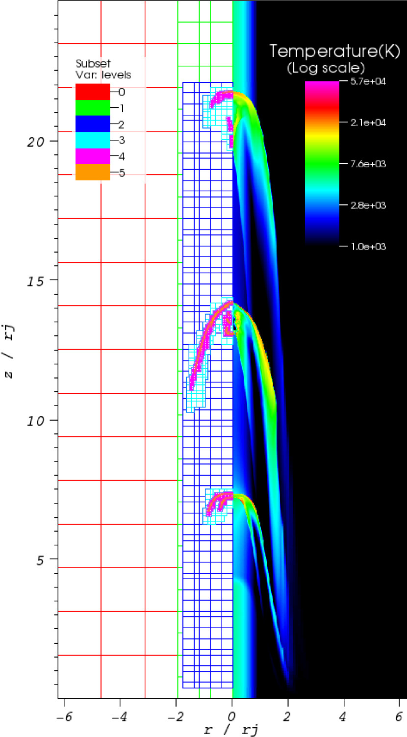
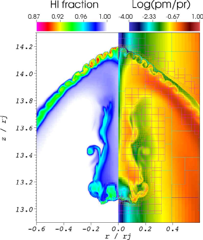
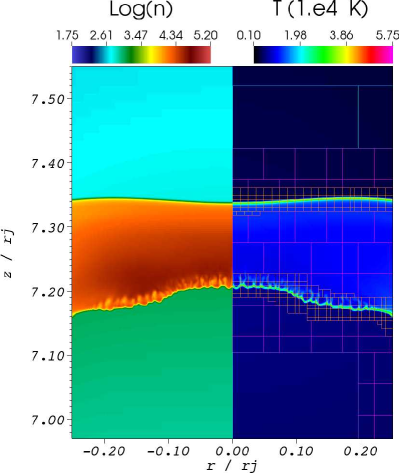
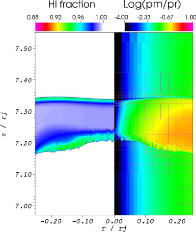
Figure 21.— Radiative jet structure at $t\approx 64.3\,{\rm yrs}$. On the left we display a full view of the temperature distribution (right) and AMR block structure (left). The smaller panels to the right show closeup views of number density (left half, in cm^-3), temperature (right half, in $10^{4}\,$ K), neutral hydrogen (left half) and magnetization $B_{\phi}^{2}/(2p)$ (right half) for the second (top panels) and third (bottom panels) shock, respectively. The AMR block structure is overplotted in the right half of each panel.

Figure 22.— One dimensional enlarged cuts at $r\approx 0.1133r_{j}$ across the middle shock in the radiative jet model at $t=64.3\,{\rm yrs}$. Temperature density distributions are plotted in the top panel while the first ionization stage of O, H, N and neutral Sulphur are plotted in the bottom panel.

Radiative jet models with a variable ejection velocity are commonly adopted to reproduce the knotty structure observed in collimated outflows from young stellar objects. The time variability leads to the formation of a chain of perturbations that eventually steepen into pairs of forward/reverse shocks (the ”internal working surfaces” see, for instance de Colle & Raga, 2006; Raga et al., 2007; Teşileanu et al., 2009) which are held responsible for the typical spectral signature of these objects. While these internal working surfaces travel down the jet, the emission from post-shocked regions occurs on a much smaller spatial and temporal scale thus posing a considerable challenge even for AMR codes.

As an example application, we solve the MHD equations coupled to the chemical network described in Teşileanu et al. (2008), evolving the time-dependent ionization and collisionally-excited radiative losses of the most important atomic/ionic species: H, He, C, N, O, Ne and S. While hydrogen and helium can be at most singly-ionized, we only consider the first three (instead of five) ionization stages of the other elements which suffices for the range of temperatures and densities considered here. This amounts to a total of 19 additional non-homogeneous continuity/rate equations such as Eq. (3).

The initial condition consists of an axisymmetric supersonic collimated beam in cylindrical coordinates $(r,z)$ in equilibrium with a stationary ambient medium. Density and axial velocity can be freely prescribed as

$$\rho(r)=\rho_{a}+\frac{\rho_{j}-\rho_{a}}{\cosh(r^{4}/r_{j}^{4})}\,,\quad v_{z}(r)=\frac{v_{j}}{\cosh(r^{4}/r_{j}^{4})}\,,\quad$$ (67)

where $\rho_{j}$ and $\rho_{a}=\rho_{j}/5$ are the jet and ambient mass density, $v_{j}=200\,{\rm km/s}$ is the jet velocity and $r_{j}=2\cdot 10^{15}\,{\rm cm}$ is the radius. The jet density is given by $\rho_{j}=n_{j}\mu_{j}m_{a}$ where $n_{j}=10^{3}$ is the total particle number density, $\mu_{j}$ is the mean molecular weight and $m_{a}$ is the atomic mass unit. Both the initial jet cross section and the environment are neutral with the exception of C and S which are singly ionized. The steady state results from a radial balance between the Lorentz and pressure forces and has to satisfy the time-independent momentum equation:

$$\frac{dp}{dr}=-\frac{1}{2}\frac{1}{r^{2}}\frac{d(rB_{\phi})^{2}}{dr}\,$$ (68)

where, for simplicity, we neglect rotations and assume a purely azimuthal magnetic field of the form

$$B_{\phi}(r)=-\frac{B_{m}}{r}\sqrt{1-\exp\left[-(r/a)^{4}\right]}\,.$$ (69)

Here $a=0.9r_{j}$ is the magnetization radius and $B_{m}$ is a constant that depends on the jet and ambient temperatures. Direct integration of Eq. (68) yields the equilibrium profile

$$p(r)=p_{j}-\frac{1}{2}\frac{B_{m}^{2}\sqrt{\pi}\,\textrm{erf}(r^{2}/a^{2})}{a^{2}}\,,$$ (70)

where $p_{j}=\rho_{j}k_{B}T_{j}/(\mu_{j}m_{a})$ is the jet pressure on the axis, $\mu_{j}$ is the mean molecular weight, $m_{a}$ is the atomic mass unit, $k_{B}$ is the Boltzmann constant and $T_{j}$ is the jet temperature. The value of $B_{m}$ is recovered by solving equation (70) in the $r\to\infty$ limit given the jet and ambient temperatures $T_{j}=5\cdot 10^{3}\,{\rm K}$ and $T_{a}=10^{3}\,{\rm K}$, respectively. Our choice of parameters is similar to the one adopted by Raga et al. (2007).

The computational domain is defined by $r/r_{j}\in[0,12.5]$, $z/r_{j}\in[0,25]$ with axisymmetric boundary conditions holding at $r=0$. At $z=0$ we keep the flow variables constant and equal to the equilibrium solution and add a sinusoidal time-variability of the jet velocity with a period of $20\,{\rm yrs}$ and an amplitude of $40\,{\rm km/s}$ around the mean value. Free-outflow is assumed on the remaining sides. We integrate the equations using linear reconstruction with the MC limiter, Eq. (34), and the HLLC Riemann solver. The time step is computed from Eq. (23, 24) using a Courant number $C_{a}=0.6$, a relative tolerance $\epsilon_{c}=0.02$ and following the considerations given in Section 4.2. Shock-adaptive hybrid integration is used by locally switching to the more diffusive MinMod limiter (Eq. 35) and the HLL Riemann solver, according to the mechanism outlined in Appendix B.

The base grid consists of $128\times 256$ zones and $5$ additional levels with grid refinement jumps of $2:2:2:4:4$ are used. At the effective resolution of $16384\times 32768$ zones the minimum length scale that can be resolved corresponds to $1.526\cdot 10^{12}\,{\rm cm}$ ($\approx 0.1$ AU), the same as model $M3$ of Raga et al. (2007). Zones are tagged for refinement when the second derivative error norm of density exceeds the threshold value $\chi_{\rm ref}=0.15$. In order to enhance the resolution of strongly emitting shocked regions, we prevent levels higher than $2$ to be created if the temperature does not exceed $5\cdot 10^{3}\times\ell$ where $\ell$ is the level number.

The results are shown, after $\approx 63.4$ years, in Figure 21 where the steepening of the perturbations leads to the formation of forward/reverse shock pairs. Radiative losses become strongly enhanced behind the shock fronts where temperature attains larger values and the compression is large. This is best illustrated in the closeup views of Fig 21 where we display density, temperature, hydrogen fraction and magnetization for the second (upper panel) and third shocks (lower panel), respectively located at $z\approx 14.2$ and $z\approx 7.34$ (in units of the jet radius). Owing to a much shorter cooling length, $t_{c}\sim p/\Lambda$, a thin radiative layer forms the size of which, depending on local temperature and density values, becomes much smaller than the typical advection scale. An extremely narrow one-dimensional cut shows, in Figure 22, the profiles of temperature, density and ionization fractions across the central radiative shock, resolved at the largest refinement level. Immediately behind the shock wave, a flat transition region with constant density and temperature is captured on $\sim 6$ grid points and has a very small thickness $\sim 0.005r_{j}$. A radiatively cooled layer follows behind where temperature drops and the gas reaches the largest ionization degree. Once the gas cools below $10^{4}$ K, radiative losses become negligible and the gas is accumulated in a cold dense adiabatic layer. A proper resolution of these thin layers is thus crucial for correct and accurate predictions of emission lines and intensity ratios in stellar jet models (Teşileanu et al., 2011). Such a challenging computational problem can be tackled only by means of adaptive grid techniques.

6. Relativistic MHD Tests

In this section we apply PLUTO-CHOMBO to test problems involving relativistic magnetized flows in one, two and three dimensions. Both standard numerical benchmarks and applications will be considered. By default, the conservative MUSCL-Hancock predictor scheme (Eq. 43) together with linear reconstruction on primitive variables are used during the computation of the normal predictors.

6.1. One dimensional Shock-Tube

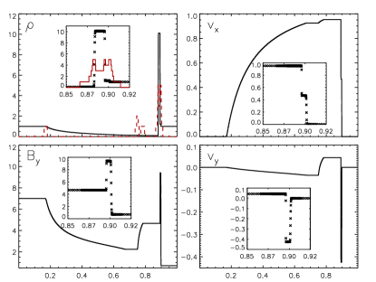
Figure 23.— Density (top left), longitudinal velocity (top right), $y$ components of magnetic field and velocity (bottom left and right) for the one-dimensional relativistic magnetized shock tube problem at t=0.4. We employ a base grid of $400$ cells with $5$ levels of refinement with consecutive jump ratios of $4:2:2:2:2$ yielding an equivalent resolution of $25600$ zones. The grid hierarchy is shown in the top left panel (dashed red line) while magnifications of the thin shell are plotted, for each quantity, using symbols in the interior plot windows.

Our first test consists of an initial discontinuity located at $x=0.5$ separating two regions of fluids characterized by

$$\left(B_{y},\,B_{z},\,p\right)=\left\{\begin{array}[]{ll}(7,\,7,\,10^{3})&\quad{\rm for}\quad x<0.5\\ \vskip 6.0pt plus 2.0pt minus 2.0pt\cr(0.7,\,0.7,\,0.1)&\quad{\rm for}\quad x>0.5\end{array}\right.$$ (71)

(see Balsara, 2001; Mignone & Bodo, 2006; van der Holst et al., 2008 and references therein). The fluid is initially at rest with uniform density $\rho=1$ and the longitudinal magnetic field is $B_{x}=10$.

We solve the equations of relativistic MHD with the ideal gas law ($\Gamma=5/3$) using the 5-wave HLLD Riemann solver of Mignone et al. (2009) and $C_{a}=0.6$. The computational domain $[0,1]$ is discretized using $5$ levels of refinement with consecutive grid jump ratios of $4:2:2:2:2$ starting from a base grid (level $0$) of $400$ grid zones (yielding an effective resolution of $25600$ zones). Refinement is triggered upon the variable $\sigma=(B_{y}^{2}+B_{z}^{2})/D$ using Eq. (50) with a threshold $\chi_{r}=0.1$. At $t=0.4$ the resulting wave pattern (Fig. 23) is comprised of two left-going rarefaction fans (fast and slow) and two right-going slow and fast shocks. The presence of magnetic fields makes the problem particularly challenging since the contact wave, slow and fast shocks propagate very close to each other, resulting in a thin relativistic blast shell between $x\approx 0.88$ and $x\approx 0.9$.

Table 3CPU performance for the one-dimensional RMHD shock-tube.

Static Run		AMR Run			Speedup
$N_{x}$	Time (s)	Level	Ref ratio	Time (s)
1600	6.1	1	4	1.8	3.4
3200	29.9	2	2	3.8	7.9
6400	124.5	3	2	8.2	15.2
12800	502.3	4	2	18.1	27.8
25600	2076.1	5	2	41.2	50.4

Note. — The first and second columns give the number of points $N_{x}$ and corresponding CPU for the static grid run (no AMR). The third, fourth and fifth columns give, respectively, the number of levels, the refinement ratio and CPU time for the AMR run at the equivalent resolution. The last column shows the corresponding speedup factor.

In Table 3 we compare, for different resolutions, the CPU timing obtained with the static grid version of the code versus the AMR implementation at the same effective resolution, starting from a base grid of $400$ zones. In the unigrid computations, halving the mesh size implies approximately a factor of four in the total running time whereas only a factor of two in the AMR approach. At the large resolution employed here, the overall gain is approximately $50$. This example confirms that the resolution of complex wave patterns in RMHD can largely benefit from the use of adaptively refined grids.

6.2. Inclined Generic Alfvén Test

Figure 24.— Horizontal cuts for the rotated inclined Alfvén test at $t=0.4/\sqrt{2}$ (symbols) and for the 1-D reference solution at $t=0.4$ (solid line). The top row shows, from left to right, proper density, gas pressure and Lorentz factor. In the middle and bottom rows we plot the components of velocity and magnetic field normal ($v_{1}$ and $B_{1}$) and transverse ($v_{2},v_{3}$ and $B_{2},B_{3}$) to the surface of discontinuity.

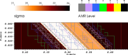
Figure 25.— A closeup of the central region in the inclined Alfvén test at $t=0.4/\sqrt{2}$ showing $\sigma=\mathbf{B}^{2}/D$ with the overplotted block distribution. The base grid has $64\times 4$ zones and $5$ levels of refinement are used.

The generic Alfvén test (Giacomazzo & Rezzolla, 2006; Mignone et al., 2009) consists of the following non planar initial discontinuity

$$\left\{\begin{array}[]{lclr}\mathbf{V}_{L}&=&\displaystyle\left(1,0,0.3,0.4,1,6,2,5\right)^{T}&\mathrm{for}\quad x_{1}<1/2\,,\\ \vskip 6.0pt plus 2.0pt minus 2.0pt\cr\mathbf{V}_{R}&=&\displaystyle\left(0.9,0,0,0,1,5,2,5.3\right)^{T}&\mathrm{for}\quad x_{1}>1/2\,,\end{array}\right.$$ (72)

where, as in Section 5.1.1, $\mathbf{V}=(\rho,v_{1},v_{2},v_{3},B_{1},B_{2},B_{3},p)$ is given in the frame of reference aligned with the direction of motion $x_{1}$. The ideal equation of state (10) with $\Gamma=5/3$ is adopted.

Here we consider a two-dimensional version by rotating the discontinuity front by $\pi/4$ with respect to the mesh and following the evolution until $t=0.4\cos\pi/4$. The test is run on a coarse grid of $64\times 4$ zones covering the domain $x\in[0,1]$, $y\in[-1/32,1/32]$ with 6 additional levels of refinement resulting in an effective resolution of $4096\times 256$ zones (a factor of 2 in resolution is used between levels). In order to trigger refinement across jumps of different nature, we define the quantity $\sigma=\mathbf{B}^{2}/D$ together with Eq. (50) and a threshold value $\chi_{r}=0.03$. The Courant number is $C_{a}=0.6$ and the HLLD Riemann solver is used throughout the computation. Boundary conditions assume zero-gradients at the $x$ boundaries while translational invariance is imposed at the top and bottom boundaries where, for any flow quantity $q$, we set $q(i,j)=q(i\pm 1,j\mp 1)$.

The breaking of the discontinuity, shown in Fig. 24, leads to the formation of seven waves including a left-going fast rarefaction, a left-going Alfvén discontinuity, a left-going slow shock, a tangential discontinuity, a right-going slow shock, a right-going Alfvén discontinuity and a right-going fast shock. Our results indicate that refined regions are created across discontinuous fronts which are correctly followed and resolved, in excellent agreement with the reference solution (obtained on a fine one-dimensional grid). Note also that the longitudinal component of the magnetic field, $B_{1}$, does not present spurious jumps (Fig. 24) and shows very small departures from the expected constant value. In the central region, for $0.4\lesssim x\lesssim 0.6$, rotational discontinuities and slow shocks are moving slowly and very adjacent to each other thus demanding relatively high resolution to be correctly captured. With the given prescription, grid adaptation efficiently provides adequate resolution where needed. This is best shown in the closeup of the central region, Fig. 25, showing $\sigma$ together with the AMR block structure.

A comparison of the performance between static and adaptive grid computations is reported in Table 4 using different resolutions and mesh refinements. At the resolution employed here, the gain is approximately a factor of $9$.

Table 4CPU performance for the two-dimensional inclined generic Alfvén test.

Static Run			AMR Run				Speedup
$N_{x}$	Time (s)		Level	Ref ratio	#Blocks	Time (s)
128	1.8		1	2	4	1.1	$1.6$
256	10.8		2	2	14	6.1	$1.8$
512	75.2		3	2	44	33.0	$2.3$
1024	557.8		4	2	126	185.9	$3.0$
2048	4390.5		5	2	306	900.0	$4.9$
4096	35250.0		6	2	761	4346.9	$8.1$

Note. — The base grid for the AMR computation is $64\times 4$ zones.

6.3. Relativistic Rotor Problem

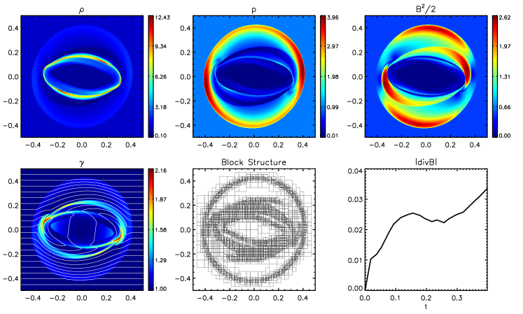
Figure 26.— The relativistic rotor problem at $t=0.4$ using $6$ levels of refinement on a base grid with $64^{2}$ zones. From left to right, top to bottom: density, gas pressure, magnetic field, density, Lorentz factor (magnetic field lines are overplotted), block distribution and domain-average of $|\nabla\cdot\mathbf{B}|$.

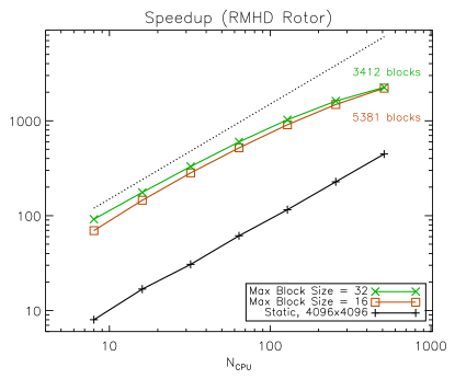
Figure 27.— Parallel scalings for the 2D relativistic rotor from 8 to 512 CPUs. The red and green lines (squares and crosses, respectively) give the speedup factors corresponding to computations with maximum block sizes of $16$ and $32$ zones, respectively. The number of blocks on the finest level ($\ell=6$) at the end of integration is reported above and below the corresponding curve. The dotted black line gives the perfect scaling.

The two-dimensional rotor problem (Del Zanna et al., 2003; van der Holst et al., 2008; Dumbser et al., 2008) consists of a rapidly spinning disk embedded in a uniform background medium ($\rho=p=1$) threaded by a constant magnetic field $\mathbf{B}=(1,0,0)$. Inside the disk, centered at the origin with radius $R=0.1$, the density is $\rho=10$ and the velocity is prescribed as $\mathbf{v}=\omega(-y,x,0)$ where $\omega=9.95$ is the angular frequency of rotation. The computational domain is the square $x,y\in[-\frac{1}{2},\frac{1}{2}]$ with outflow (i.e. zero-gradient) boundary conditions. Computations are performed on a base grid with $64^{2}$ grid points and $6$ levels of refinement using the HLL Riemann solver and a CFL number $C_{a}=0.5$. Zones are tagged for refinement whenever the second derivative error norm of ${\cal E}/(\rho\gamma)$, computed with (50), exceeds $\chi_{r}=0.15$. The effective resolution amounts therefore to $4096^{2}$ zones, the largest employed so far (to the extent of our knowledge) for this particular problem.

Results are shown at $t=0.4$ in Fig. 26 where one can see an emerging flow structure enclosed by a circular fast forward shock ($r\approx 0.425$) traveling into the surrounding medium. An inward fast shock bounds the innermost oval region where density has been depleted to lower values. The presence of the magnetic field slows down the rotor and the maximum Lorentz factor decreases from $10$ to $\approx 2.2$. The numerical solution preserves the initial point symmetry and density corrugations, present in lower resolution runs, seem drastically reduced at this resolution, in accordance with the findings of van der Holst et al. (2008). Divergence errors are mostly generated in proximity of the outer fast shock and are damped while being transported out of the domain at the speed of light in the GLM formulation. We monitor the growth of such errors by plotting the volume-average of $|\nabla\cdot\mathbf{B}|$ as a function of time showing (bottom panel in Fig. 26) that the growth of monopole errors is limited to the same values of van der Holst et al. (2008) (the factor of $4$ comes from the fact that our computational domain is twice as small).

Parallel performance for this particular test is shown in Fig. 27 plotting the speedup, defined as $S=8T^{\rm u}_{8}/T_{N_{\rm CPU}}$, where $T^{\rm u}_{8}$ is the execution time of the uniform grid run performed at the same effective resolution ($4096^{2}$) on $8$ processors while $T_{N_{\rm CPU}}$ is the running time measured with $N_{\rm CPU}$ processors. AMR scaling has been quantified for computations using maximum patch sizes of $16$ and $32$ grid points resulting, respectively, in $11921$ and $6735$ total number of blocks at the end of integration. Approximately half of it belongs to the finest level, as reported in Fig 27. In general, the AMR approach offers a $5$ to $10$ speedup gain in terms of execution time over the uniform, static grid approach. For $N_{\rm CPU}<256$ the parallel efficiency, measured as $S/N_{\rm CPU}$, is larger than $0.7$ while it tends to be reduced for more processors. Computations carried with fewer blocks (i.e. larger block sizes) tend to be more efficient when fewer CPUs are in use since inter-processor communications are reduced. However, this cost becomes sensibly larger at $512$ (or more) processors resulting in a loss of efficiency.

6.4. Cylindrical Blast Wave

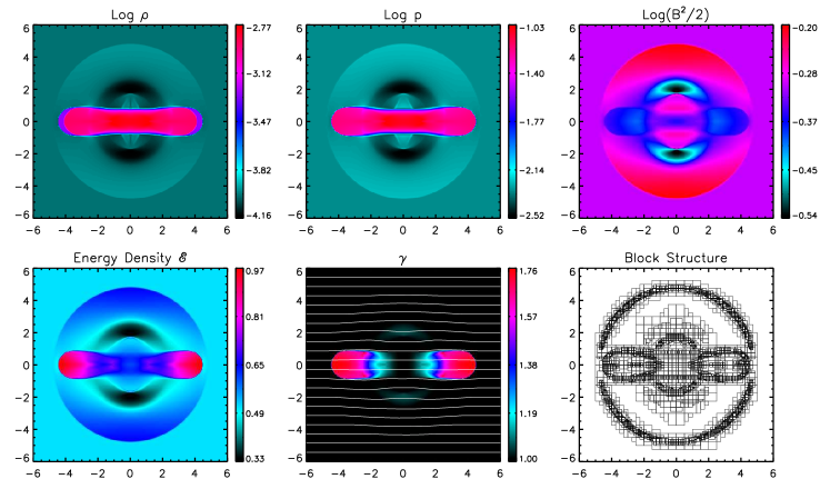
Figure 28.— Cylindrical relativistic blast wave at $t=4$. The base level grid has $48^{2}$ zones and $5$ levels of refinement are used. The different maps show proper density (top left, log scale), thermal pressure (top right) magnetic field strength (top right, log scale) density (bottom left, log scale) and Lorentz factor (bottom right). Refinement levels $3$ and $4$ are overplotted on the first plot while magnetic field lines overlap in the latter.

Strong symmetric explosions in highly magnetized environments can become rather arduous benchmarks probing the code’s ability to evolve strongly magnetized shocks (see, for instance Komissarov, 1999; Leismann et al., 2005; Mignone & Bodo, 2006; Del Zanna et al., 2003; Beckwith & Stone, 2011). Failures may lead to unphysical densities or pressures whenever the scheme does not introduce adequate dissipation across oblique discontinuities and/or if the divergence-free condition is not properly controlled.

The two dimensional setup considered here consists of the Cartesian square $[-6,6]\times[-6,6]$ initially filled with constant density and pressure values $\rho=10^{-4}$ and $p=5\cdot 10^{-3}$ and threaded by a constant horizontal magnetic field with strength $B_{0}=1$. A cylinder with radius $r=0.8$ and centered at the origin delimits a higher density and pressure region where $\rho=10^{-2}$, $p=1$. The ideal EoS with with $\Gamma=4/3$ is used. Our choice of parameters results in a low $\beta$ plasma ($2p/B^{2}=10^{-2}$) and corresponds to the strongly magnetized cylindrical explosion discussed by Beckwith & Stone (2011). We point out that this configuration differs from the one discussed in Komissarov (1999) and Mignone & Bodo (2006) by having the ambient pressure ten times larger. This allows to run the computation without having to introduce any specific change or modification in the algorithm, such as shock flattening or redefinition of the total energy. We adopt a base grid of $48$ zones in each direction with outflow boundary conditions holding on all sides. Integration proceeds until $t=4$ using the HLLC Riemann solver (Mignone & Bodo, 2006) using $5$ levels of refinement, reaching an effective resolution of $1536^{2}$ zones. Total energy triggers refinement with a threshold of $\chi_{\rm ref}=0.025$.

The over-pressurized region, Fig. 28, sets an anisotropic blast wave delimited by a weak fast forward shock propagating almost radially. The explosion is strongly confined along the $x$ direction by the magnetic field where plasma is accelerated to $\gamma_{\max}\approx 1.76$. The inner structure is delimited by an elongated structure enclosed by a slow shock adjacent to a contact discontinuity. The two fronts blend together as the propagation becomes perpendicular to the field line. Since the problem is purely two dimensional, rotational discontinuties are absent. The block distribution, shown in the lower panel of Fig. 28, shows that refinement clusters around the outer discontinuous wave as well as the multiple fronts delimiting the extended inner region. The total number of blocks is $2258$ with the finest level giving a relative contribution of $\sim 0.55$ and a corresponding volume filling factor of $\sim 0.12$. The numerical solution retains the expected degree of symmetry and the agreement with earlier results demonstrate the code can robustly handle strongly magnetized relativistic shocks within the GLM-MHD formalism. Results obtained with $4$ processors show that calculation done with AMR is faster than the static grid runs by a factor of $\sim 4.5$.

6.5. Spherical Blast Wave

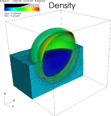
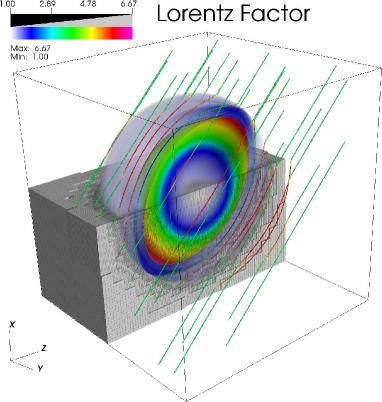
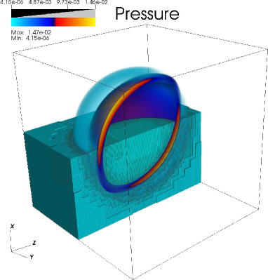
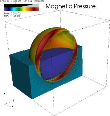
Figure 29.— Density slice-cut for the relativistic magnetized blast wave in three dimensions at $t=4$. Four levels of refinement are used to achieve an effective resolution of $640^{3}$. The box in the lower half-semispace emphasize jump ratios across levels. Oblique magnetic fieldlines are overplotted.

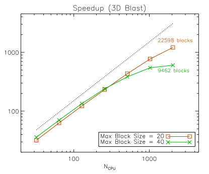
Figure 30.— Parallel scalings for the three-dimensional relativistic blast wave problem from 32 to 2048 processors. The red and green lines (squares and crosses, respectively) give the speedup factors corresponding to ”frozen-flux” computations with maximum block sizes of $20$ and $40$ zones, respectively. The number of blocks on the finest level, reported above and below each line, stays constant in time. Ideal scaling is given by the dotted black line.

In the next example we consider a three-dimensional extension of the cylindrical blast wave problem presented in Del Zanna et al. (2007). The initial condition consists of a sphere with radius $r=0.8$ centered at the origin filled with hot gas having $\rho=10^{-2}$, $p=1$ (the ideal EoS with $\Gamma=4/3$ is used). Outside this region, density and pressure decrease linearly reaching the constant ambient values $\rho=10^{-4}$, $p=5\cdot 10^{-3}$ for $r\geq 1$. The plasma is at rest everywhere and a constant magnetic field is set oblique to the mesh, i.e., $\mathbf{B}=B_{0}(\hat{\mathbf{e}}_{x}+\hat{\mathbf{e}}_{y})/\sqrt{2}$ with $B_{0}=0.1$. The computational domain is the Cartesian box $[-6,6]^{3}$ covered by a base grid of $40$ zones in each direction with outflow boundary conditions holding on all sides. Using the HLLD Riemann solver, we follow integration until $t=4$ using $4$ levels of refinement (effective resolution $640^{3}$) and a CFL number $C_{a}=0.4$. Zones are tagged for refinement upon density fluctuations with a threshold value of $\chi_{\rm ref}=0.15$.

Results shown in Figure 29 reveal an oval-shaped explosion enclosed by an outer fast shock propagating almost radially. A strong reverse shock confines a prolate spheroidal region where magnetic field has been drained and inside which expansion takes place radially. The largest Lorentz factor $\sim 6.3$ is attained in the direction of magnetic field lines close to the ellipsoid poles.

In order to measure parallel performance on a fixed number of blocks, we have integrated the solution array starting from $t=3.5$ for a fixed number of steps by enforcing zero interface flux. Results are shown in Fig. 30 where we compare two sets of ”frozen-flux” computations with maximum block sizes of 20 and 40 mesh points corresponding, respectively, to 27661 (22598 on the finest level) and 11229 (9462 on the finest level) total number of blocks. In the former case, the larger number of patches allows to reach a better efficiency (more than $0.75$) whereas the latter case performs worse for increasing number of processors. Even if the finest level has a number of blocks still larger than the maximum number of CPUs employed, many boxes are much smaller than the maximum block size allowed. The ideal workload per processor (i.e. the number of cells of the finest level divided by the number of processors) is comparable to the maximum block size in the 1024 CPUs run and becomes smaller in the 2048 CPUs run. In this latter case, the workload of the processors integrating the larger blocks is therefore larger than the ideal one and most of the CPUs must wait for these processors to complete the integration. This could explain the poor parallel performance of this case.

6.6. Kelvin-Helmholtz flow

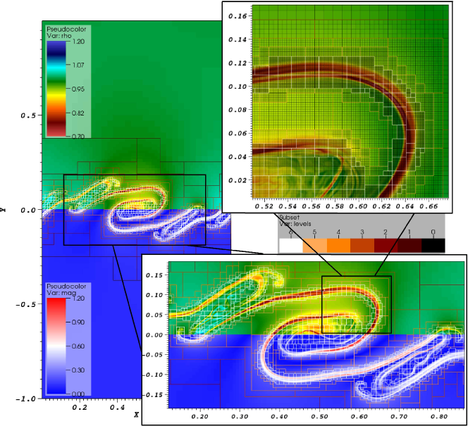
Figure 31.— Relativistic Kelvin-Helmholtz instability at $t=5$ using $6$ additional levels of refinement starting from a base grid of $32\times 64$. The panel on the left shows density (upper half) and the quantity $(B_{x}^{2}+B_{y}^{2})^{\frac{1}{2}}/B_{z}$ (lower half) on the whole computational domain. Selected regions are enlarged in the two panels on the right.

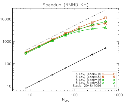
Figure 32.— Parallel speedup up to 512 processors for the two-dimensional relativistic Kelvin-Helmholtz instability problem. Speedup is computed as the ratio $8T_{8}^{u}/T_{N_{\rm CPU}}$ between the execution time of the static uniform grid run at the same effective resolution ($2048\times 4096$) on $8$ processors and the running time measured with $N_{\rm CPU}$ processors. Red lines corresponds to the 3-level run using max grid sizes of 16 (squares) and 32 (crosses). Green lines corresponds the the 6-level compuations.

In the next example (Bucciantini & Del Zanna, 2006; Mignone et al., 2009) we consider a two-dimensional planar domain with $x\in[0,1]$, $y\in[-1,1]$ initially filled with a (relativistically) hot gas with constant density $\rho=1$ and pressure $p=20$. An initially perturbed shear velocity profile of the form

$$(v_{x},v_{y},v_{z})=\left[V_{0}\tanh\frac{y}{\alpha},\epsilon\sin(2\pi x)\exp\left(-\frac{y^{2}}{\beta^{2}}\right),0\right]$$ (73)

is set across the domain, where $V_{0}=1/4$ is the nominal flow velocity, $\epsilon=V_{0}/100$ is the amplitude of the perturbation while $\alpha=0.01$, $\beta=0.1$. The TM equation of state, Eq. (11), is used during the evolution to recover the gas enthalpy from density and pressure. The magnetic field is initially uniform and prescribed in terms of the components parallel and perpendicular to the plane of integration:

$$(B_{x},B_{y},B_{z})=\left(\sqrt{2\sigma_{\rm pol}p},0,\sqrt{2\sigma_{\rm tor}p}\right)$$ (74)

where $\sigma_{\rm pol}=0.01$, $\sigma_{\rm tor}=1$. We perform the integration on a base grid of $32\times 64$ cells with $6$ additional levels of refinement, reaching an effective resolution of $2048\times 4096$ zones. The Courant number is set to $C_{a}=0.8$ and refinement is triggered whenever Eq. (50) computed with total energy density exceeds $\chi_{r}=0.14$. Open boundary conditions hold at the lower and upper $y$ boundaries while periodicity is imposed in the $x$ direction.

Fig. 31 shows density and magnetic field distributions at $t=5$ which approximately marks the transition from the linear phase to the nonlinear evolution (see the discussion in Mignone et al., 2009). Both density and magnetic field are organized into filaments that wrap around forming a number of vortices arranged symmetrically with respect to the central point. Refined levels concentrate mainly around the location of the fluid interface and accurately follow the formation of the central vortex and the more elongated adjacent ones. The computation preserves the initial point-symmetry even if the grid generation algorithm does not necessarily do so. The lower resolution outside this region contributes to damp acoustic waves as they travel towards the outer boundaries and eventually reduces the amount of spurious reflections.

In Fig. 32 we compare the parallel speedup between a number of adaptive grid calculations using either $6$ levels (grid jump of 2) or $3$ levels (grid jump of 4) and the equivalent uniform grid run with $2048\times 4096$ zones. Generally, the AMR approach is $\approx 40$ faster than the fixed grid run. In addition, the 3-level computation seems to perform somewhat better than the 6-level run although the number of blocks on the finest levels is essentially the same at the end of computation (1085 and 1021, respectively). Parallel scaling sensibly deteriorates when the number of blocks per processor becomes less than $3$ or $4$, in accordance with the results of previous tests.

6.7. Three dimensional Shock-Cloud Interaction

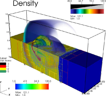
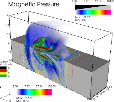
Figure 33.— Vertical cut in the $xz$ plane showing the interaction of a magnetized relativistic shock with a density cloud at $t=1$. Density and magnetic pressure $\mathbf{B}^{2}/2$ are shown in the left and right panels, respectively. For each quantity, a volumetric rendering is shown in the upper half whereas an intensity color map in the middle vertical and horizontal planes displays below. The base grid corresponds to $64\times 32^{2}$ and $4$ levels of refinement are employed (effective resolution $1024\times 512^{2}$).

In the next example we consider a three-dimensional extension of the planar relativistic shock-cloud interaction originally presented in Mignone & Bodo (2006). The initial condition consists of a high density ($\rho=10$) spherical clump (radius $0.15$) centered at $(0.8,0,0)$ adjacent to a shock wave located at $x=0$ with downstream and upstream values given by $(\rho,v_{x},B_{z},p)=(42.5942,\,0,\,-2.12971,\,127.9483)$ for $x<0$ and $(\rho,v_{x},B_{z},p)=(1,\,-\sqrt{0.99},\,0.5,\,10^{-3})$ for $x\geq 0$. The remaining quantities are set to zero. The computational domain is the box $x\in[0,2]$, $y,z\in[-\frac{1}{2},\frac{1}{2}]$. At the base level we fix the resolution to $64\times 32\times 32$ zones and employ $4$ levels of refinement equivalent to an effective resolution of $1024\times 512\times 512$. The refinement criterion (50) uses the conserved density for zone tagging with a threshold $\chi_{r}=0.2$. The equations of relativistic MHD are solved using the TM EoS (Mignone & McKinney, 2007), the HLLD Riemann solver and linear reconstruction with the harmonic limiter (41). Shock adaptive hybrid integration provides additional numerical dissipation in proximity of strong shock waves by switching the integration scheme to the HLL Riemann solver and the MinMod limiter (Eq. 35), according to the strategy described in Appendix B. For efficiency purposes, we take advantage of the symmetry across the $xy$ and $xz$ planes to reduce the computation to one quadrant only.

Fig. 33 shows a three-dimensional rendering of density and magnetic pressure through a cross-sectional view of the $xy$ and $xz$ planes at $t=1$. The collision generates a fast, forward bow shock propagating ahead and a backward reverse shock transmitted back into the cloud. The cloud becomes gradually wrapped by the incident shock into a mushroom-shaped shell reaching a large compression ($\rho_{\max}\approx 121$, $\mathbf{B}^{2}/2\approx 157$). Grid refinement concentrates mainly around the incident and forward shocks and the tangential discontinuities bordering the edge of the cloud.

6.8. Propagation of Three-dimensional Relativistic Magnetized Jet

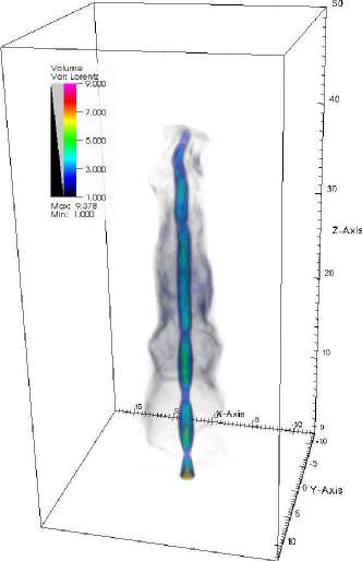
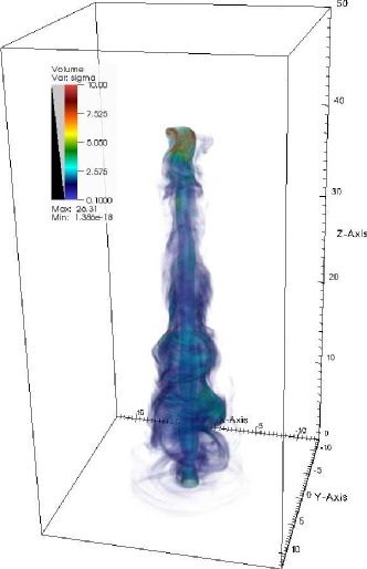
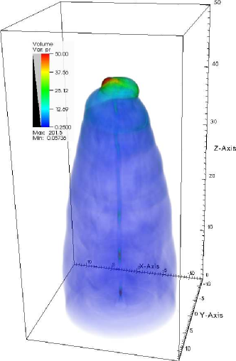
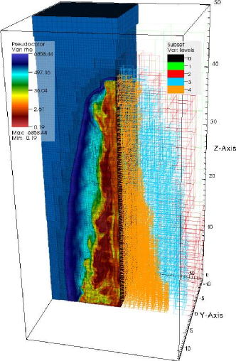
Figure 34.— Three dimensional visualization of the relativistic magnetically dominated jet at $t=130$ using 4 levels of refinement. In the top panels we show the distribution of the Lorentz factor (left) and magnetic to kinetic energy ratio $|\mathbf{B}|^{2}/(\gamma^{2}\rho)$ (right). In the bottom panels we show the thermal pressure distribution (left) and a slice cut of density together with the grid structure (right).

As a final application, we discuss the three-dimensional propagation of a relativistic magnetized jet carrying an initially purely azimuthal magnetic field. Indeed, the presence of a substantial toroidal component of the field is commonly invoked and held responsible for the acceleration and collimation of jets from active galactic nuclei. If on one hand cylindrical MHD configuration are expected to be unstable to reflection, Kelvin-Helmholtz and current driven modes, on the other hand astrophysical jets appear to be quite stable thus posing an unsolved issue, see Mignone et al. (2010) and reference therein.

Following Mignone et al. (2009) we set the box $x,y\in[-12.5,12.5]$, $z\in[0,50]$ as our computational domain, initially filled with constant uniform density and pressure $\rho_{a}$ and $p_{a}$. The beam is injected at the lower boundary for $z\leq 0$, $r=\sqrt{x^{2}+y^{2}}\leq 1$ with a density $\rho_{j}$, a longitudinal velocity corresponding to a Lorentz factor $\gamma_{j}$ and an azimuthal magnetic field given by

$$B_{\phi}=\left\{\begin{array}[]{ll}\gamma_{j}b_{m}r/a&\quad{\rm for}\quad r<a\,,\\ \vskip 6.0pt plus 2.0pt minus 2.0pt\cr\gamma_{j}b_{m}a/r&\quad{\rm for}\quad a<r<1\,,\\ \vskip 6.0pt plus 2.0pt minus 2.0pt\cr 0&\quad{\rm otherwise}\,,\end{array}\right.$$ (75)

where $b_{m}$ is the magnetic field strength in the fluid’s frame and $a=0.5$ is the magnetization radius. The pressure profile is found by imposing radial momentum balance across the beam giving

$$p(r)=p_{a}+b_{m}^{2}\left[1-\min\left(\frac{r^{2}}{a^{2}},1\right)\right]\,,$$ (76)

where $p_{a}$ is the ambient pressure defined in terms of the sonic Mach number $M$:

$$p_{a}=\frac{\rho_{j}v_{j}^{2}(\Gamma-1)}{\Gamma(\Gamma-1)M^{2}-\Gamma v_{j}^{2}}\,,$$ (77)

with $\Gamma=5/3$ although the TM equation of state (11) is used during the evolution. The actual value of $b_{m}$ may be found by prescribing the magnetization parameter $\sigma_{\phi}$ defined as the ratio between beam-averaged magnetic energy density and thermal pressure. The final result yields (Mignone et al., 2009):

$$b_{m}=\sqrt{\frac{-4p_{a}\sigma_{\phi}}{a^{2}(2\sigma_{\phi}-1+4\log a)}}\,.$$ (78)

For the present simulation we adopt $\gamma_{j}=7$, $M=3$, $\sigma_{\phi}=1.3$, $\rho_{j}=1$ and $\rho_{a}=10^{3}$ thus corresponding to a magnetically dominated, underdense relativistic jet.

We follow the simulation up to $t=130$ (in units of the speed of light crossing of the jet radius), starting with a base grid of $32\times 32\times 64$ with $4$ levels of refinement. The refinement ratio between consecutive levels is 2 so that, at the finest resolution, we have $\approx 20$ points per beam radius. Zones belonging to levels 0,1 and 2 are tagged for refinement using the normalized second-derivative Eq. (50) of the total energy density with a threshold $\chi_{r}=0.25$. Zones at the finest level grid are instead created by using $\mathbf{B}^{2}/(\gamma\rho)$ in place of the total energy density. The rationale for choosing this selective rule is to provide the largest resolution on the jet material only, still being able to track the sideway expansion of the cocoon at lower resolution. We use the HLLD Riemann solver with the harmonic limiter (41) except at strong shocks where we employ the multidimensional shock dissipation switch outlined in Appendix B. The Courant number is $C_{a}=0.3$.

The jet structure, Fig. (34), shows that the flow maintains a highly relativistic central spine running through multiple recollimation shocks where jet pinching occurs. At the jet head the beam decelerates to sub-relativistic velocities favoring the formation of a strongly magnetized termination shock where $\mathbf{B}^{2}\approx 26\gamma^{2}\rho$. Here, the presence of a predominant toroidal magnetic field induces current driven (CD) kink instability which are responsible for the observed jet wiggling and symmetry breaking (see Mignone et al., 2010). This test shows that PLUTO-CHOMBO can be effectively used in simulations involving relativistic velocities, highly supersonic flows and strongly magnetized environments.

At $t=130$ the finest level grid has a volume filling factor of $\approx 11$ per cent with 10761 blocks while level $3$ occupies $\approx 41$ per cent of the total volume with 5311 blocks. For this particular application, the benefits offered by grid adaptivity are more evident at the beginning of the computation when most of the computational zones in the domain are unrefined. In this respect, we have found that the CPU time increases (for $t\leq 130$) with the number of steps $n$ approximately as $a+bn+cn^{2}+dn^{3}$ where $a\approx 1.46$, $b\approx 0.079$, $c\approx 5.03\cdot 10^{-4}$ and $d\approx 2.38\cdot 10^{-6}$. This suggests that, as long as the filling factor remains well below $1$, the AMR calculation with the proposed refinement criterion should be at least $\sim 2.5$ times faster than an equivalent computation using static mesh refinement and considerably larger if compared to a uniform grid run at the effective resolution.

7. Summary

In this paper, we have presented a cell-centered implementation of the PLUTO code for multi-dimensional adaptive mesh refinement (AMR) computations targeting Newtonian and relativistic magnetized flows. A block structured approach has been pursued by taking full advantage of the high-level parallel distributed infrastructure available in the CHOMBO library. This choice provides the necessary level of abstraction in delivering AMR functionality to the code allowing, at the same time, full compatibility with most of the modular implementations already available with the static grid version. This eases up the process of adding or replacing physics modules as long as they comply with the interface requirements.

A novel extension to incorporate diffusion terms such as viscosity, resistivity and heat conduction without the need for operator splitting, has been illustrated in the context of the dimensionally unsplit corner transport upwind (CTU) time stepping scheme. In addition, the scheme has also been extended to the realm of relativistic MHD (RMHD) using a characteristic projection-free, MUSCL-Hancock normal predictor step. The integration scheme retains second-order spatial and temporal accuracy requiring 6 Riemann solvers per cell per step. Interface states are calculated using the piecewise parabolic method (PPM) integration although alternatives based on weighted essentially non-oscillatory (WENO) or linear slope-limited schemes are also available. The proposed cell-centered version of PLUTO-CHOMBO enforces the divergence-free condition by augmenting the system of equations with a generalized Lagrange multiplier (GLM, see Dedner et al., 2002), in the implementation outlined by Mignone & Tzeferacos (2010). The choice of the GLM-MHD formalism has proven to be a convenient starting point in porting a significant fraction of the static grid code implementations to the AMR framework. Although future extensions will also consider other strategies to enforce the $\nabla\cdot\mathbf{B}=0$ condition, the proposed formulation offers substantial ease of implementation and a viable robust alternative to a constrained transport approach which typically requires additional care for prolongation and restriction operations at fine-coarse interfaces (see, for instance, Balsara, 2001, 2004; Cunningham et al., 2009).

A suite of several test problems including standard numerical benchmarks and astrophysical applications for MHD and RMHD has been selected to assess the efficiency of PLUTO-CHOMBO in resolving complex flow patterns viable through an adaptive grid approach in 1, 2 and 3 dimensions. Examples include simple shock-tube problems, resistive sheets, radiative and thermally conducting flows, fluid instabilities and blast wave explosions in highly magnetized environments. The computational saving offered by an adaptive grid computation has been shown, for many of the selected test, to be several times or even order of magnitudes faster than a static grid integration. Parallel performance, evaluated for some of the proposed tests, suggests good scalability properties for two- and three-dimensional problems as long as the number of grids per processor is larger than a factor between $2$ and $3$.

Both the static and AMR version of PLUTO are distributed as a single software package publicly available at http://plutocode.ph.unito.it/ while the CHOMBO library can be freely downloaded from https://seesar.lbl.gov/anag/chombo/. The AMR version of PLUTO has been designed to retain salient features characterizing the static grid version (Mignone et al., 2007) such as modularity - the possibility to easily combine different numerical schemes to treat different physics-, portability and user-friendliness. While stable code releases along with extensive documentation and benchmarks are made available on the WEB, the code is being actively developed and future development will address additional new physical aspects as well as improved numerical algorithms.

Appendix A Discretization of the Thermal Conduction Flux

The discretization of the heat conduction flux, Eq. (6), reflects the mixed parabolic/hyperbolic mathematical nature of the underlying differential operators, as anticipated in Section 2.1.1. From the diffusion limit, $|\mathbf{F}_{\rm class}|/q\to 0$, we compute $\mathbf{F}_{\rm class}$ at cell interfaces using second-order accurate central difference expressions for $\nabla T$, e.g., at constant $x$-faces,

$$\left.\frac{\partial T}{\partial x}\right|_{i+\frac{1}{2}}\approx\frac{T_{i+1,j}-T_{i,j}}{\Delta x}\,,\qquad\left.\frac{\partial T}{\partial y}\right|_{i+\frac{1}{2}}\approx\frac{(T_{i+1,j+1}+T_{i,j+1})-(T_{i+1,j-1}+T_{i,j-1})}{4\Delta y}$$ (A1)

and similarly at constant $y$- and $z$- faces. In the purely hyperbolic limit, $|\mathbf{F}_{\rm class}|/q\to\infty$, we see that $\mathbf{F}_{c}\to q\hat{\mathbf{t}}$ where $\hat{\mathbf{t}}=\mathbf{F}_{\rm class}/|\mathbf{F}_{\rm class}|$ is a unit vector in the direction of the heat flux. To gain more insights, we re-write the one-dimensional energy equation in this limit by keeping only pressure-related terms, that is,

$$\frac{\partial}{\partial t}\left(\frac{p}{\gamma-1}\right)-\frac{\partial}{\partial x}\left(5\phi\rho c_{\rm iso}^{3}t_{x}\right)=0\,,$$ (A2)

where $c_{\rm iso}=\sqrt{p/\rho}$ is the isothermal speed of sound and $t_{x}=\hat{\mathbf{e}}_{x}\cdot\hat{\mathbf{t}}$. Equation (A2) is a nonlinear advection equation of the form $\partial_{t}u+\partial_{x}f=0$ where $u=p/(\gamma-1)$ and $f=-qt_{x}$ is the hyperbolic saturated flux. A stable discretization is therefore provided by adopting an upwind scheme (Balsara et al., 2008) such as

$$q_{i+\frac{1}{2}}=\left\{\begin{array}[]{ll}\displaystyle\frac{5\phi}{\sqrt{\rho_{i+\frac{1}{2}}}}p_{L}^{3/2}&\qquad{\rm if}\quad t_{x}<0\,,\\ \vskip 6.0pt plus 2.0pt minus 2.0pt\cr\displaystyle\frac{5\phi}{\sqrt{\rho_{i+\frac{1}{2}}}}p_{R}^{3/2}&\qquad{\rm otherwise}\,.\\ \vskip 6.0pt plus 2.0pt minus 2.0pt\cr\end{array}\right.\qquad$$ (A3)

In the previous equation $\rho_{i+\frac{1}{2}}=(\rho_{L}+\rho_{R})/2$, $p_{L}$ and $p_{R}$ are computed from the left/right input states for the Riemann problem. Finally, we define the thermal conduction flux at constant $x$-faces (for instance) as the harmonic mean between the two regimes,

$$\left(\hat{\mathbf{e}}_{x}\cdot\mathbf{F}_{c}\right)_{i+\frac{1}{2}}=\frac{q_{i+\frac{1}{2}}}{|\mathbf{F}_{\rm class}|_{i+\frac{1}{2}}+q_{i+\frac{1}{2}}}\left(\hat{\mathbf{e}}_{x}\cdot\mathbf{F}_{\rm class}\right)_{i+\frac{1}{2}}$$ (A4)

where $q_{i+\frac{1}{2}}$ is computed from Eq. (A3).

Appendix B Multidimensional Shock Detection and Adaptive Hybrid-Integration

In regions of strong shocks or gradients spurious numerical oscillations may arise and quickly lead to the occurrence of unphysical states characterized, for example, by negative pressures, energies, densities or, in the case of relativistic flows, superluminal speeds. Such episodes are usually limited to very few grid zones and are originated by either insufficient numerical diffusion or lack of a physical solution of the Riemann problem.

To circumvent this potential hitch, PLUTO provides a safeguard built-in mechanism that i) flag zones that may potentially reside inside a strong shock wave and ii) introduces additional numerical dissipation by locally replacing the integration scheme with a more diffusive one. For these reasons, most of the interpolation schemes and Riemann solvers available with PLUTO embody a hybrid selective mechanism that allows to switch, if required, to a more dissipative choice. This process is controlled by a 3D array of integers where each element represents a set of flags that can be individually turned on or off by simple bitwise operations. Zones are flagged according to a flexible shock-detection criterion,

$$\frac{\left|\Delta_{x}q\right|}{\min\left(q_{i+1},q_{i-1}\right)}+\frac{\left|\Delta_{y}q\right|}{\min\left(q_{j+1},q_{j-1}\right)}+\frac{\left|\Delta_{z}q\right|}{\min\left(q_{k+1},q_{k-1}\right)}>\epsilon_{q}\qquad{\rm\emph{and}}\qquad\nabla\cdot\mathbf{v}<0\,,$$ (B1)

where $\Delta_{d}$ is a standard central difference operator, $q$ is thermal (default) or magnetic pressure, $\mathbf{v}$ is the velocity and $\epsilon_{q}$ is a free adjustable parameter (default is 5). The first condition detects zones within a strong gradient while the second one is switched on where compressive motion takes place. When both conditions are met, we flag the zone $\{i,j,k\}$ to be updated with the HLL Riemann solver. At the same time we also flag all neighboring zones whose interpolation stencil includes the shocked zone to be interpolated using slope-limited reconstruction with the MinMod limiter. We note that both flags may be selected and combined independently and, in any case, preserve the second-order accuracy of the scheme.

References

- Balsara (2001) Balsara, D. S. 2001, J. Comput. Phys., 174, 614
- Balsara (2001) Balsara, D. S. 2001, ApJS, 132, 83
- Balsara (2004) Balsara, D. S. 2004, ApJS, 151, 149
- Balsara & Shu (2000) Balsara, D. S., & Shu, C.-W. 2000, J. Comput. Phys., 160, 405
- Balsara et al. (2008) Balsara, D. S., Tilley, D. A., & Howk, J. C. 2008, MNRAS, 386, 627
- Beckwith & Stone (2011) Beckwith, K., & Stone, J. M. 2011, ApJS, 193, 6
- Berger & Colella (1989) Berger, M. J., & Colella, P. 1989, J. Comput. Phys., 82, 64
- Berger & Oliger (1984) Berger, M. J. & Oliger, J. 1984, J. Comput. Phys., 53, 484
- Berger & Rigoutsos (1995) Berger, M. J., & Rigoutsos, I. 1991, IEEE Transactions on Systems, Man and Cybernetics, 21, 1278
- Birn et al. (2001) Birn, J., Drake, J. F., Shay, M. A., et al. 2001, J. Geophys. Res., 106, 3715
- Biskamp (1986) Biskamp, D. 1986, Physics of Fluids, 29, 1520
- Brio & Wu (1988) Brio, M., & Wu, C. C. 1988, J. Comput. Phys., 75, 400
- Bucciantini & Del Zanna (2006) Bucciantini, N., & Del Zanna, L. 2006, A&A, 454, 393
- Cassak & Drake (2009) Cassak, P. A., & Drake, J. F. 2009, ApJ, 707, L158
- Colella & Woodward (1984) Colella, P., & Woodward, P. R. 1984, J. Comput. Phys., 54, 174
- Colella (1990) Colella, P. 1990, J. Comput. Phys., 87, 171
- Cowie & McKee (1977) Cowie, L. L., & McKee, C. F. 1977, ApJ, 211, 135
- Cunningham et al. (2009) Cunningham, A. J., Frank, A., Varnière, P., Mitran, S., & Jones, T. W. 2009, ApJS, 182, 519
- Dai & Woodward (1994) Dai, W., & Woodward, P.R. 1994, ApJ, 436, 776
- de Colle & Raga (2006) de Colle, F., & Raga, A. C. 2006, A&A, 449, 1061
- Dedner et al. (2002) Dedner, A., Kemm, F., Kröner, D., et al. 2002, J. Comput. Phys., 175, 645
- Del Zanna et al. (2003) Del Zanna, L., Bucciantini, N. & Londrillo, P. 2003, A&A, 400, 397
- Del Zanna et al. (2007) Del Zanna, L., Zanotti, O., Bucciantini, N., & Londrillo, P. 2007, A&A, 473, 11
- Dezeeuw & Powell (1993) Dezeeuw, D., & Powell, K. G. 1993, J. Comput. Phys., 104, 56
- Dumbser et al. (2008) Dumbser, M., Balsara, D. S., Toro, E. F. & Munz, C.-D. 2008, J. Comput. Phys., 227, 8209
- Fromang et al. (2006) Fromang, S., Hennebelle, P., & Teyssier, R. 2006, A&A, 457, 371
- Fryxell et al. (2000) Fryxell, B., et al. 2000, ApJS, 131, 273
- Gammie et al. (2003) Gammie, C. F., McKinney, J. C., & Tóth, G. 2003, ApJ, 589, 444
- Gardiner & Stone (2005) Gardiner, T. A., & Stone, J. M. 2005, J. Comput. Phys., 205, 509
- Gardiner & Stone (2008) Gardiner, T. A., & Stone, J. M. 2008, J. Comput. Phys., 227, 4123
- Giacomazzo & Rezzolla (2006) Giacomazzo, B., & Rezzolla, L. 2006, J. Fluid Mech., 562, 223-259
- Ji et al. (1998) Ji, H., Yamada, M., Hsu, S., & Kulsrud, R. 1998, Physical Review Letters, 80, 3256
- Jiang & Shu (1996) Jiang, G. S., & Shu, C.-W. 1996, J. Comput. Phys., 126, 202-228.
- Keppens et al. (2003) Keppens, R., Nool, M., Tóth, G., & Goedbloed, J. P. 2003, Comput. Phys. Comm., 153, 317
- Keppens et al. (2008) Keppens, R., Meliani, Z., van der Holst, B., & Casse, F. 2008, A&A, 486, 663
- Khokhlov (1998) Khokhlov, A. M. 1998, J. Comput. Phys., 220, 678
- Komissarov (1999) Komissarov, S. S. 1999, MNRAS, 303, 343
- Lee & Deane (2009) Lee, D., & Deane, A. E. 2009, J. Comput. Phys., 228, 952
- Leismann et al. (2005) Leismann, T., Antón, L., Aloy, M. A., et al. 2005, A&A, 436, 503
- Löhner (1987) Löhner, R. 1987, Computer Methods in Applied Mechanics and Engineering, 61, 323
- MacNeice et al. (2000) MacNeice, P., Olson, K. M., Mobarry, C., de Fainchtein, R., & Packer, C. 2000, Comput. Phys. Comm., 126, 330
- Massaglia et al. (2005) Massaglia, S., Mignone, A., & Bodo, G. 2005, A&A, 442, 549
- Mathews (1971) Mathews, W. G. 1971, ApJ, 165, 147
- Mignone et al. (2005) Mignone, A., Plewa, T., & Bodo, G. 2005, ApJS, 160, 199
- Mignone & Bodo (2006) Mignone, A., & Bodo, G. 2006, MNRAS, 368, 1040
- Mignone et al. (2007) Mignone, A., Bodo, G., Massaglia, S., et al. 2007, ApJS, 170, 228 (Paper I)
- Mignone & McKinney (2007) Mignone, A., & McKinney, J. C. 2007, MNRAS, 378, 1118
- Mignone et al. (2009) Mignone, A., Ugliano, M., & Bodo, G. 2009, MNRAS, 393, 1141
- Mignone & Tzeferacos (2010) Mignone, A., & Tzeferacos, P. 2010, J. Comput. Phys., 229, 2117 (MT)
- Mignone et al. (2010) Mignone, A., Tzeferacos, P. & Bodo, G. 2010, J. Comput. Phys., 229, 5896
- Mignone et al. (2010) Mignone, A., Rossi, P., Bodo, G., Ferrari, A., & Massaglia, S. 2010, MNRAS, 402, 7
- Miller & Colella (2002) Colella, P., & Miller, G. H. 2002, J. Comput. Phys., 183, 26
- Mizuno et al. (2006) Mizuno, Y., Nishikawa, K.-I., Koide, S., Hardee, P., & Fishman, G. J. 2006, arXiv:astro-ph/0609004
- Orlando et al. (2008) Orlando, S., Bocchino, F., Reale, F., Peres G., & Pagano, A. 2008, ApJ, 678, 274
- Parker (1957) Parker, E. N. 1957, J. Geophys. Res., 62, 509
- Pember et al. (1996) Pember, R. B., Greenough, J. A. & Colella, P. 1996, Tech. Report UCRLJC-123351
- Raga et al. (2007) Raga, A. C., de Colle, F., Kajdič, P., Esquivel, A., & Cantó, J. 2007, A&A, 465, 879
- Reynolds et al. (2006) Reynolds, D. R., Samtaney, R., & Woodward, C. S. 2006, J. Comput. Phys., 219, 144
- Rider et al. (2007) Rider, W. J., Greenough, J. A., & Kamm J. R. 2007, J. Comput. Phys., 225, 1827
- Ryu & Jones (1995) Ryu, D., & Jones, T. W. 1995, ApJ, 442, 228
- Skinner & Ostriker (2010) Skinner, M. A., & Ostriker, E. C. 2010, ApJS, 188, 290
- Stone & Gardiner (2007) Stone J. M., & Gardiner, T. 2007, Physics of Fluids, 19, 094104
- Stone et al. (2008) Stone, J. M., Gardiner, T. A., Teuben, P., Hawley, J. F., & Simon, J. B. 2008, ApJS, 178, 137
- Sweet (1958) Sweet, P. A. 1958, Electromagnetic Phenomena in Cosmical Physics, 6, 123
- Teşileanu et al. (2008) Teşileanu, O., Mignone, A., & Massaglia, S. 2008, A&A, 488, 429
- Teşileanu et al. (2009) Teşileanu, O., Massaglia, S., Mignone, A., Bodo, G., & Bacciotti, F. 2009, A&A, 507, 581
- Teşileanu et al. (2011) Teşileanu, O., Mignone, A., Massaglia, S., & Bacciotti, F. 2011, ApJ, submitted
- Teyssier (2002) Teyssier, R. 2002, A&A, 385, 337
- Torrilhon (2003) Torrilhon, M. 2003, J. Comput. Phys., 192, 73
- Torrilhon & Balsara (2004) Torrilhon, M., & Balsara, D. S. 2004, J. Comput. Phys., 201, 586
- Tóth (1996) Tóth, G. 1996, Astrophysical Letters Communications, 34, 245
- Tóth (2000) Tóth, G. 2000, J. Comput. Phys., 161, 605
- Tóth et al. (2008) Tóth, G., Ma, Y., & Gombosi, T. I. 2008, J. Comput. Phys., 227, 6967
- Tóth et al. (2011) Tóth, G. et al., 2011, J. Comput. Phys., in press
- Uzdensky & Kulsrud (2000) Uzdensky, D. A., & Kulsrud, R. M. 2000, Physics of Plasmas, 7, 4018
- van Albada et al. (1982) van Albada, G. D., Van Leer, B., & Roberts, W. W., 1982, A&A, 108, 76
- van der Holst & Keppens (2007) van der Holst, B., & Keppens, R. 2007, J. Comput. Phys., 226, 925
- van der Holst et al. (2008) van der Holst, B., Keppens, R., & Meliani, Z. 2008, Comput. Phys. Comm., 179, 617
- van Leer (1974) van Leer, B., 1974, J. Comput. Phys., 14, 361
- Van Straalen (2009) Van Straalen, B., Shalf, J., Ligocki T., et al. 2009, in IPDPS 2009, IEEE Computer Society
- Yamaleev & Carpenter (2009) Yamaleev, N. K., & Carpenter, M. H. 2009, J. Comput. Phys., 228, 3025
- Ziegler (2008) Ziegler, U. 2008, Comput. Phys. Comm., 179, 227
- Zhang & MacFadyen (2006) Zhang, W., & MacFadyen, A. I. 2006, ApJS, 164, 255