Induced vacuum energy-momentum tensor in
the background of a cosmic string

Abstract

A massive scalar field is quantized in the background of a cosmic string which is generalized to a static flux-carrying codimension-2 brane in the locally flat multidimensional space-time. We find that the finite energy-momentum tensor is induced in the vacuum. The dependence of the tensor components on the brane flux and tension, as well as on the coupling to the space-time curvature scalar, is comprehensively analyzed. The tensor components are holomorphic functions of space dimension, decreasing exponentially with the distance from the brane. The case of the massless quantized scalar field is also considered, and the relevance of Bernoulli’s polynomials of even order for this case is discussed.

Keywords: vacuum polarization, vortex, multidimensional conical space-time

1 Introduction

String-like configurations of classical background fields can polarize the vacuum of quantized matter fields, resulting in the emergence of a nonzero vacuum expectation value of the energy-momentum tensor in spatial regions where the classical field is zero. A particular example of a string-like configuration is a tube of the magnetic flux lines, that is formed inside a current-carrying long and thin solenoid. But a more general string-like structure is the Abrikosov-Nielsen-Olesen vortex [1, 2] arising as a topological defect in the aftermath of a phase transition with spontaneous breakdown of a continuous symmetry; the condition of its arising is that the first homotopy group of the group space of the broken symmetry group be nontrivial. The vortex, apart from its flux, is characterized by nonzero energy distributed along its axis, which in its turn, according to general relativity, is a source of gravity. It can be shown [3, 4, 5] that this source makes space outside the vortex to be conical with the deficit angle related to the energy density per unit length of the vortex. Since the squared Planck length enters as a factor before the stress-energy tensor in the Einstein-Hilbert equation, the deviations from the Minkowskian metric are of the order of squared quotient of the Planck length to the correlation length, the latter characterizing the thickness of the vortex. For superconductors this quotient is vanishingly small and effects of conicity are surely negligible [6]; hence, the appropriate vortices known as the Abrikosov ones are much the same as the solenoidal magnetic vortices (with one important distinction that the flux of the former is quantized). However, topological defects of the vortex type arise in cosmology under the name of cosmic strings [7, 8]. Cosmic strings with the thickness of the order of the Planck length are definitely ruled out by astrophysical observations, and there remains a room for cosmic strings with the thickness which is more than 3.5 orders larger than the Planck length, that corresponds to the deficit angles bounded from above by the value of $2.5\times 10^{-6}$ radians (see [9]). Cosmic strings associated with spontaneous breakdown of global symmetries are called global (or axionic) strings; they are characterized by zero flux. Cosmic strings associated with breakdown of gauge symmetries are called gauge (or local) strings; they are characterized by nonzero flux.

Cosmic strings can have various astrophysical effects, in particular, they serve as plausible sources of detectable gravitational waves [10, 11, 12], gamma-ray bursts [13], high-energy cosmic rays [14]. Although the primary role of cosmic strings in the formation of the large-scale structure of the Universe is ruled out by observation of cosmic microwave background by COBE and WMAP [15, 16], cosmic strings can produce a mechanism for the generation of the primordial magnetic field in the early Universe [17, 18, 19]. The interest to cosmic strings is augmented in the last decade owing to the finding that they emerge at the end of inflation in the framework of superstring models [20, 21] (see also reviews [22, 23, 24, 25]). The details of the cosmic string formation mechanism can be quite different, either fundamental (super)strings or Dirichlet branes are stretched to a macroscopic size, but such structures arize almost inevitably in supergravity models with large extra dimensions [26]. In this respect it is appropriate to consider a generalization of a cosmic string in 4-dimensional space-time to a codimension-2 brane in higher-dimensional space-time. Such a brane appears also in the construction of brane-world cosmologies with two extra dimensions (see [27, 28, 29] and references therein), as well as in the study of quantum aspects of the black hole physics, playing a key role in the formation of chains of Kaluza-Klein bubbles with black holes [30, 31]. Therefore, the properties of the vacuum of quantized matter in the background of a codimension-2 brane deserve investigation.

A study of the vacuum polarization effects in the cosmic string background has a long history. The induced vacuum energy-momentum tensor was considered for the cases of global [32, 33, 34] and gauge [35, 36] strings; in the above the quantized fields were assumed to be massless, whereas the results for the nonvanishing mass were either incomplete or of restricted use, see [37, 38, 39]. The effects of nonvanishing mass were exhaustively studied for the case of a negligible deficit angle only [40] (see also [41, 42]). In this respect it should be noted that the induced vacuum current in the cosmic string background is known both in the massive [19] and massless [43] cases.

The aim of the present paper is to obtain the energy-momentum tensor which is induced in the vacuum of the quantized massive scalar field in the cosmic string background. In the next section, the vacuum expectation value of the energy-momentum tensor is in general defined with the use of the point-splitting regularization. Green’s function in the cosmic string background is obtained in section 3. The induced vacuum energy-momentum tensor is obtained in section 4. Some limiting cases of our result are discussed in section 5, while the case of the massless quantized scalar field is considered in section 6. The results are summarized in section 7. We relegate the details of derivation of Green’s function in the cosmic string background to the appendix.

2 Energy-momentum tensor: point-splitting regularization

The energy-momentum tensor for the quantized charged massive scalar field $\Psi(x)$ is given by expression [44, 45] (for a review see [46])

$$T^{\mu\nu}(x)=\frac{1}{2}\left[\nabla^{\mu}\Psi^{\dagger}(x),\,\nabla^{\nu}\Psi(x)\right]_{+}+\frac{1}{2}\left[\nabla^{\nu}\Psi^{\dagger}(x),\,\nabla^{\mu}\Psi(x)\right]_{+}$$

$$+\frac{1}{4}g^{\mu\nu}\left[(\Box+m^{2}+\xi R)\Psi^{\dagger}(x),\,\Psi(x)\right]_{+}+\frac{1}{4}g^{\mu\nu}\left[\Psi^{\dagger}(x),\,(\Box+m^{2}+\xi R)\Psi(x)\right]_{+}$$

$$+(\xi-\frac{1}{4})g^{\mu\nu}\Box\left[\Psi^{\dagger}(x),\,\Psi(x)\right]_{+}-\xi\left(\nabla^{\mu}\nabla^{\nu}+R^{\mu\nu}\right)\left[\Psi^{\dagger}(x),\,\Psi(x)\right]_{+},$$ (1)

where $\nabla_{\mu}$ is the covariant derivative involving both affine and bundle connections, $\Box=\nabla_{\mu}\nabla^{\mu}$ is the covariant d’Alembertian operator, $g_{\mu\nu}$ is the space-time metric tensor, $R^{\mu\nu}$ is the Ricci tensor and $R=g_{\mu\nu}R^{\mu\nu}$ is the scalar curvature of space-time, $\xi$ is the coupling constant of the scalar field to the space-time scalar curvature. The product of the field operators at the same point $(x)$ is ill-defined, and this leads to the divergence of the formal expression for the vacuum expectation value of the energy-momentum tensor, $\langle 0|T^{\mu\nu}(x)|0\rangle$. To regularize this divergence, one uses the point splitting for the operator product in (1):

$$T^{\mu\nu}(x;\,x^{\prime})=D^{\mu\nu}(x;\,x^{\prime})\left[T\Psi(x)\Psi^{\dagger}(x^{\prime})+T\Psi(x^{\prime})\Psi^{\dagger}(x)\right],$$ (2)

where $T$ is the symbol of chronological ordering in the operator product and

$$D^{\mu\nu}(x;\,x^{\prime})=\left(\frac{1}{2}-\xi\right)\left(\nabla^{\mu}_{x}\nabla^{\nu}_{x^{\prime}}+\nabla^{\nu}_{x}\nabla^{\mu}_{x^{\prime}}\right)$$

$$+\xi g^{\mu\nu}(\Box_{x}+m^{2}+\xi R_{x})+\xi g^{\mu\nu}(\Box_{x^{\prime}}+m^{2}+\xi R_{x^{\prime}})$$

$$+2\left(\xi-\frac{1}{4}\right)g^{\mu\nu}\left(g_{\rho\sigma}\nabla_{x}^{\rho}\nabla_{x^{\prime}}^{\sigma}-m^{2}-\frac{1}{2}\xi R_{x}-\frac{1}{2}\xi R_{x^{\prime}}\right)$$

$$-\xi\left(\nabla_{x}^{\mu}\nabla_{x}^{\nu}+\nabla_{x^{\prime}}^{\mu}\nabla_{x^{\prime}}^{\nu}+\frac{1}{2}R_{x}^{\mu\nu}+\frac{1}{2}R_{x^{\prime}}^{\mu\nu}\right).$$ (3)

The vacuum expectation value of tensor $T^{\mu\nu}$ (2) is well defined. Further, if field operator $\Psi$ obeys the Klein-Gordon equation, then the vacuum expectation value of the chronological operator product in the right-hand side of (2) is related to Green’s function of the Klein-Gordon operator,

$$\langle 0|T\Psi(x)\Psi^{\dagger}(x^{\prime})|0\rangle=-{\rm i}G(x;\,x^{\prime}),$$ (4)

where

$$\left(\Box_{x}+m^{2}+\xi R_{x}\right)G(x;\,x^{\prime})=\left(\Box_{x^{\prime}}+m^{2}+\xi R_{x^{\prime}}\right)G(x;\,x^{\prime})=\frac{1}{\sqrt{g}}\delta(x-x^{\prime})$$ (5)

and $g=|{\rm det}g_{\mu\nu}|$. Green’s function is decomposed as

$$G(x;\,x^{\prime})=G(x;\,x^{\prime})_{(S)}+G(x;\,x^{\prime})_{(R)},$$ (6)

where the first term is singular, whereas the second one is regular in the coincidence limit, $x^{\prime}\rightarrow x$; the divergence of the vacuum expectation value of tensor $T^{\mu\nu}$ (1) is due to the contribution of $G(x;\,x^{\prime})_{(S)}+G(x^{\prime};\,x)_{(S)}$ to tensor $T^{\mu\nu}$ (2). Thus, the physically meaningful (renormalized) vacuum expectation value of the energy-momentum tensor is obtained by taking the coincidence limit after the subtraction of the dangerous (divergent in this limit) part:

$$t^{\mu\nu}(x)=-{\rm i}\lim\limits_{x^{\prime}\rightarrow x}D^{\mu\nu}(x;\,x^{\prime})\left[G(x;\,x^{\prime})_{(R)}+G(x^{\prime};\,x)_{(R)}\right].$$ (7)

This is a quite general scheme which is only necessary but not sufficient to define unambiguously the renormalized value. As we shall see in the next section, to get the renormalized value in the case of the cosmic string background, it suffices to subtract the appropriate value in the case of the trivial (Minkowski) background.

3 Cosmic string background: Green’s function

As is already mentioned, a cosmic string associated with spontaneous breakdown of a gauge symmetry is characterized by a gauge field with the strength which is directed along the string and is non vanishing inside its core; the total flux of the strength is denoted in the following by $\Phi$. Space-time outside the string core is the conical space-time where a surface orthogonal to the string axis is isometric to the surface of a cone; the deficit angle is $8\pi G\mu$, where $G$ is the gravitational constant (squared Planck length), $\mu$ is the tension (or energy density per unit length) of the string, and units $c=\hbar=1$ are used. In view of the significance of high-dimensional space-times in various aspects [24, 25], we consider a generalization of a cosmic string to a codimension-2 brane in $(d+1)$-dimensional space-time with squared length element

$${\rm d}s^{2}={\rm d}t^{2}-{\rm d}r^{2}-\nu^{-2}r^{2}{\rm d}\varphi^{2}-{\rm d}{\bf z}^{2}_{d-2},$$ (8)

where $r$ and $\varphi$ are the polar coordinates of the conical surface, ${\bf z}_{d-2}=(x^{3},\,\ldots,\,x^{d})$, $x^{j}$ ($j=\overline{3,\,d}$) are the Cartesian coordinates of flat ($d-2$)-dimensional space, and

$$\nu=(1-4G\mu)^{-1}.$$ (9)

The transverse size of the cosmic string is neglected, and both the spatial and the bundle curvatures are nonvanishing and singular (as distributions) in the codimension-2 brane (i.e. point in the $d=2$ case, line in the $d=3$ case, surface in the $d=4$ case and $(d-2)$-hypersurface in the $d>4$ case). Thus, the cosmic string background in which the scalar matter field is quantized is characterized by two dimensionless parameters: $4G\mu$ and $e\Phi(2\pi)^{-1}$, where $e$ is the coupling constant of the scalar to the gauge field forming the string and should not be mistaken for the electromagnetic coupling constant.

The d’Alembertian in the cosmic string background takes form

$$\Box=\partial_{t}^{2}-\Delta^{({\rm tr})}-\sum\limits_{j=3}^{d}\partial_{j}^{2},$$ (10)

where

$$\Delta^{({\rm tr})}=r^{-1}\partial_{r}r\partial_{r}+\nu^{2}r^{-2}\left(\partial_{\varphi}-{\rm i}\frac{e\Phi}{2\pi}\right)^{2}$$ (11)

is the twodimensional (transverse) Laplacian and $\partial_{j}=\frac{\partial}{\partial x^{j}}$. Green’s function in the cosmic string background obeys equations

$$(\Box_{x}+m^{2})G\left(t,\,r,\,\varphi,\,{\bf z}_{d-2};\,t^{\prime},\,r^{\prime},\,\varphi^{\prime},\,{\bf z}_{d-2}^{\prime}\right)$$

$$=(\Box_{x^{\prime}}+m^{2})G\left(t,\,r,\,\varphi,\,{\bf z}_{d-2};\,t^{\prime},\,r^{\prime},\,\varphi^{\prime},\,{\bf z}_{d-2}^{\prime}\right)$$

$$=\delta(t-t^{\prime})\frac{\nu}{r}\delta(r-r^{\prime})\Delta(\varphi-\varphi^{\prime})\delta^{(d-2)}\left({\bf z}_{d-2}-{\bf z}_{d-2}^{\prime}\right),$$ (12)

where $\Delta(\varphi)=(2\pi)^{-1}\sum\limits_{n\in\mathbb{Z}}e^{in\varphi}$ is the delta-function for the angular variable, $\Delta(\varphi+2\pi)=\Delta(\varphi)$, $\mathbb{Z}$ is the set of integer numbers. It should be noted that, apart from the overall phase factor, Green’s function is periodic in the value of gauge flux $\Phi$ with the period equal to $2\pi\,e^{-1}$, i.e. it depends on

$$F=\frac{e\Phi}{2\pi}-\lshad\frac{e\Phi}{2\pi}\rshad,$$ (13)

where $\lshad u\rshad$ denotes the integer part of quantity $u$ (i.e. the integer which is less than or equal to $u$). Imposing physically plausible conditions on Green’s function at small and large distances from the string, we solve (12) unambiguously and obtain the following expression (see appendix):

$$G\left(t,\,r,\,\varphi,\,{\bf z}_{d-2};\,t^{\prime},\,r^{\prime},\,\varphi^{\prime},\,{\bf z}_{d-2}^{\prime}\right)=\frac{{\rm i}m^{(d-1)/2}}{(2\pi)^{(d+1)/2}}\exp\left[\frac{{\rm i}e\Phi}{2\pi}(\varphi-\varphi^{\prime})\right]\left[\sum\limits_{l}e^{2{\rm i}lF\pi}\right.$$

$$\times\left.\frac{K_{(d-1)/2}\left(m\sqrt{-(t-t^{\prime})^{2}+(r-r^{\prime})^{2}+\left({\bf z}_{d-2}-{\bf z}_{d-2}^{\prime}\right)^{2}+4rr^{\prime}\sin^{2}\left[(\varphi-\varphi^{\prime}+2\pi l)(2\nu)^{-1}\right]}\right)}{\left\{-(t-t^{\prime})^{2}+(r-r^{\prime})^{2}+\left({\bf z}_{d-2}-{\bf z}_{d-2}^{\prime}\right)^{2}+4rr^{\prime}\sin^{2}[(\varphi-\varphi^{\prime}+2\pi l)(2\nu)^{-1}]\right\}^{(d-1)/4}}\right.$$

$$\left.-\frac{\nu}{2\pi}\int\limits_{0}^{\infty}{\rm d}u\,\,\Omega_{\nu}^{F}(u,\,\varphi-\varphi^{\prime})\right.$$

$$\left.\times\frac{K_{(d-1)/2}\left(m\sqrt{-(t-t^{\prime})^{2}+(r-r^{\prime})^{2}+\left({\bf z}_{d-2}-{\bf z}_{d-2}^{\prime}\right)^{2}+4rr^{\prime}\cosh^{2}(u/2)}\right)}{\left[-(t-t^{\prime})^{2}+(r-r^{\prime})^{2}+\left({\bf z}_{d-2}-{\bf z}_{d-2}^{\prime}\right)^{2}+4rr^{\prime}\cosh^{2}(u/2)\right]^{(d-1)/4}}\right],$$ (14)

where the summation is over integers $l$ that satisfy condition

$$\frac{\varphi^{\prime}-\varphi}{2\pi}-\frac{\nu}{2}<l<\frac{\varphi^{\prime}-\varphi}{2\pi}+\frac{\nu}{2},$$ (15)

$K_{\alpha}(u)$ is the Macdonald function of order $\alpha$, and

$$\Omega_{\nu}^{F}(u,\,\varphi)=\frac{1}{\rm i}\left\{\frac{e^{{\rm i}(1-F)(\varphi+\nu\pi)}\cosh(F\nu u)-e^{-{\rm i}F(\varphi+\nu\pi)}\cosh[(1-F)\nu u]}{\cosh(\nu u)-\cosh(\varphi+\nu\pi)}\right.$$

$$\left.-\frac{e^{{\rm i}(1-F)(\varphi-\nu\pi)}\cosh(F\nu u)-e^{-{\rm i}F(\varphi-\nu\pi)}\cosh[(1-F)\lambda u]}{\cosh(\nu u)-\cos(\varphi-\nu\pi)}\right\}.$$ (16)

It should be emphasized that the coincidence limit, $x^{\prime}\rightarrow x$, is to be understood as limit $\varphi^{\prime}\rightarrow\varphi$ taken before the coincidence limit of at least another one variable, say, before $r^{\prime}\rightarrow r$. In this case the singularity of (14) (term corresponding to $l=0$) at $x^{\prime}\rightarrow x$ coincides with that of Green’s function in the Minkowski space-time

$$G\left.\left(t,\,r,\,\varphi,\,{\bf z}_{d-2};\,t^{\prime},\,r^{\prime},\,\varphi^{\prime},\,{\bf z}^{\prime}_{d-2}\right)\right|_{\mu=0\atop\Phi=0}=\frac{{\rm i}m^{(d-1)/2}}{(2\pi)^{(d+1)/2}}$$

$$\times\frac{K_{(d-1)/2}\left(m\sqrt{-(t-t^{\prime})^{2}+(r-r^{\prime})^{2}+({\bf z}_{d-2}-{\bf z}_{d-2}^{\prime})^{2}+4rr^{\prime}\sin^{2}[(\varphi-\varphi^{\prime})/2]}\right)}{\left\{-(t-t^{\prime})^{2}+(r-r^{\prime})^{2}+({\bf z}_{d-2}-{\bf z}_{d-2}^{\prime})^{2}+4rr^{\prime}\sin^{2}[(\varphi-\varphi^{\prime})/2]\right\}^{(d-1)/4}};$$ (17)

note that the leading singularity is independent of mass:

$$\frac{{\rm i}}{4\pi^{(d+1)/2}}\Gamma\left(\frac{d-1}{2}\right)\frac{1}{|x-x^{\prime}|^{d-1}}$$

(here $\Gamma(u)$ is the Euler gamma function). Thus, omitting the term corresponding to $l=0$ in (14) in the coincidence limit corresponds to subtracting (17) in the coincidence limit from (14), and this renormalization procedure yields finite (renormalized) vacuum expectation values.

4 Cosmic string background: renormalized vacuum energy-momentum tensor

The $l\neq 0$ terms in the finite sum in (14), as well as the last term given by an integral in (14), contribute to the renormalized vacuum expectation value of the energy-momentum tensor. Its calculation is simplified by noting the following properties:

$$(\partial_{t}+\partial_{t^{\prime}})G(x;\,x^{\prime})=0,$$

$$(\partial_{j}+\partial_{j^{\prime}})G(x;\,x^{\prime})=0,$$ (18)

$$(\partial_{\varphi}+\partial_{\varphi^{\prime}})G(x;\,x^{\prime})=0.$$

In the coincidence limit we get

$$\lim\limits_{x^{\prime}\rightarrow x}\partial_{t}G(x;\,x^{\prime})_{(R)}=\lim\limits_{x^{\prime}\rightarrow x}\partial_{j}G(x;\,x^{\prime})_{(R)}=0,$$ (19)

and, consequently, the following off-diagonal components of the induced vacuum energy-momentum tensor are vanishing:

$$t^{01}=t^{02}=t^{0j}=t^{1j}=t^{2j}=t^{jj^{\prime}}=0\,\,\,\,(j^{\prime}\neq j).$$ (20)

Due to the next relation in the coincidence limit,

$$\lim\limits_{x^{\prime}\rightarrow x}(\partial_{r}-\partial_{r^{\prime}})G(x;\,x^{\prime})_{(R)}=0,$$ (21)

the remaining off-diagonal component is vanishing as well:

$$t^{12}=0.$$ (22)

Further, since the Klein-Gordon equation is satisfied by Green’s function at $x\neq x^{\prime}$, the following relations are valid:

$$\left(g_{\rho\sigma}\nabla_{x}^{\rho}\nabla_{x^{\prime}}^{\sigma}-m^{2}\right)G(x;\,x^{\prime})=-\left[\partial_{r}\partial_{r^{\prime}}+\frac{1}{2}\left(r^{-1}\partial_{r}r\partial_{r}+{r^{\prime}}^{-1}\partial_{r^{\prime}}r^{\prime}\partial_{r^{\prime}}\right)\right]G(x;\,x^{\prime}),$$ (23)

$$\nabla^{\varphi}\nabla^{\varphi}G(x;\,x^{\prime})=g^{\varphi\varphi}\left(-\partial_{t}^{2}+\sum\limits_{j=3}^{d}\partial_{j}^{2}+r^{-1}\partial_{r}r\partial_{r}-m^{2}\right)G(x;\,x^{\prime}).$$ (24)

In view of the above, we get

$$D^{00}(x;\,x^{\prime})=-\partial_{t}^{2}-2\left(\xi-\frac{1}{4}\right)\left(\partial_{r}\partial_{r^{\prime}}+r^{-1}\partial_{r}r\partial_{r}\right),$$ (25)

$$D^{11}(x;\,x^{\prime})=\frac{1}{2}\partial_{r}\partial_{r^{\prime}}-\frac{1}{2}\partial_{r}^{2}+2\left(\xi-\frac{1}{4}\right)r^{-1}\partial_{r},$$ (26)

$$D^{22}(x;\,x^{\prime})=\nu^{2}r^{-2}\left[-\partial_{t}^{2}+\sum\limits_{j=3}^{d}\partial_{j}^{2}+2\left(\xi+\frac{1}{4}\right)r^{-1}\partial_{r}r\partial_{r}+2\left(\xi-\frac{1}{4}\right)\partial_{r}\partial_{r^{\prime}}-m^{2}\right],$$ (27)

$$D^{jj}(x;\,x^{\prime})=-\partial_{j}^{2}+2\left(\xi-\frac{1}{4}\right)\left(\partial_{r}\partial_{r^{\prime}}+r^{-1}\partial_{r}r\partial_{r}\right).$$ (28)

Applying (25)-(28) to the regular part of Green’s function according to (7) and taking the coincidence limit, we obtain the renormalized vacuum expectation value of the energy-momentum tensor:

$$t^{\mu^{\prime}}_{\mu}=q^{\mu^{\prime}}_{\mu}+s^{\mu^{\prime}}_{\mu},$$ (29)

where

$$q_{0}^{0}(r)=q_{j}^{j}(r)=-\frac{4}{(4\pi)^{(d+1)/2}}\left(\frac{m}{r}\right)^{(d+1)/2}\sum\limits_{l=1}^{\lshad\nu/2\rshad}\cos(2lF\pi)\left(\sin\frac{l\pi}{\nu}\right)^{(3-d)/2}\Biggl{\{}\Biggl{[}\left(\sin\frac{l\pi}{\nu}\right)^{-2}\Biggr{.}\Biggr{.}$$

$$\Biggl{.}\Biggl{.}+2(1-4\xi)\Biggr{]}K_{(d+1)/2}\left(2mr\sin\frac{l\pi}{\nu}\right)-2(1-4\xi)mr\sin\frac{l\pi}{\nu}K_{(d+3)/2}\left(2mr\sin\frac{l\pi}{\nu}\right)\Biggr{\}},$$ (30)

$$q_{1}^{1}(r)=-\frac{4}{(4\pi)^{(d+1)/2}}\left(\frac{m}{r}\right)^{(d+1)/2}\sum\limits_{l=1}^{\lshad\nu/2\rshad}\cos(2lF\pi)\left(\sin\frac{l\pi}{\nu}\right)^{(3-d)/2}$$

$$\times\left[\left(\sin\frac{l\pi}{\nu}\right)^{-2}-4\xi\right]K_{(d+1)/2}\left(2mr\sin\frac{l\pi}{2}\right),$$ (31)

$$q_{2}^{2}(r)=-\frac{4}{(4\pi)^{(d+1)/2}}\left(\frac{m}{r}\right)^{(d+1)/2}\sum\limits_{l=1}^{\lshad\nu/2\rshad}\cos(2lF\pi)\left(\sin\frac{l\pi}{\nu}\right)^{(3-d)/2}$$

$$\times\left[\left(\sin\frac{l\pi}{\nu}\right)^{-2}-4\xi\right]\left[K_{(d+1)/2}\left(2mr\sin\frac{l\pi}{2}\right)-2mr\sin\frac{l\pi}{\nu}K_{(d+3)/2}\left(2mr\sin\frac{l\pi}{\nu}\right)\right],$$ (32)

$$s^{0}_{0}(r)=s^{j}_{j}(r)=\frac{16\nu}{(4\pi)^{(d+3)/2}}\left(\frac{m}{r}\right)^{(d+1)/2}\int\limits_{1}^{\infty}{\rm d}v\,\Lambda(v;\,F,\,\nu)\frac{v^{(3-d)/2}}{\sqrt{v^{2}-1}}$$

$$\times\left\{[v^{-2}+2(1-4\xi)]K_{(d+1)/2}(2mrv)-2(1-4\xi)mrvK_{(d+3)/2}(2mrv)\right\},$$ (33)

$$s^{1}_{1}(r)=\frac{16\nu}{(4\pi)^{(d+3)/2}}\left(\frac{m}{r}\right)^{(d+1)/2}\int\limits_{1}^{\infty}{\rm d}v\,\Lambda(v;\,F,\,\nu)\frac{v^{(3-d)/2}}{\sqrt{v^{2}-1}}(v^{-2}-4\xi)K_{(d+1)/2}(2mrv),$$ (34)

$$s^{2}_{2}(r)=\frac{16\nu}{(4\pi)^{(d+3)/2}}\left(\frac{m}{r}\right)^{(d+1)/2}\int\limits_{1}^{\infty}{\rm d}v\,\Lambda(v;\,F,\,\nu)\frac{v^{(3-d)/2}}{\sqrt{v^{2}-1}}(v^{-2}-4\xi)$$

$$\times\left[K_{(d+1)/2}(2mrv)-2mrvK_{(d+3)/2}(2mrv)\right],$$ (35)

and

$$\Lambda(v;\,F,\,\nu)\equiv\frac{1}{2}\Omega_{\nu}^{F}(2\,{\rm arccosh}\,v,\,0)$$

$$=\frac{\sin(F\nu\,\pi)\cosh[2(1-F)\nu\,{\rm arccosh}v]+\sin[(1-F)\nu\,\pi]\cosh(2F\nu\,{\rm arccosh}v)}{\cosh(2\nu\,{\rm arccosh}v)-\cos(\nu\,\pi)};$$

(36)

clearly, tensor $q_{\mu}^{\mu^{\prime}}$ is zero for $0<\nu<2$.

One can verify that relation

$$\partial_{r}t^{1}_{1}(r)+r^{-1}\left[t^{1}_{1}(r)-t^{2}_{2}(r)\right]=0$$ (37)

is valid; hence, the induced vacuum energy-momentum tensor is conserved:

$$\nabla_{\mu}t^{\mu}_{\mu^{\prime}}=0.$$ (38)

Taking the trace of the tensor, we get

$$g_{\mu\mu^{\prime}}q^{\mu\mu^{\prime}}=-\frac{8}{(4\pi)^{(d+1)/2}}\left(\frac{m}{r}\right)^{(d-1)/2}\sum\limits_{l=1}^{\lshad\nu/2\rshad}\cos(2lF\pi)\left(\sin\frac{l\pi}{\nu}\right)^{(1-d)/2}$$

$$\times\left\{4d(\xi_{c}-\xi)\frac{m}{r}\sin\frac{l\pi}{\nu}\left[K_{(d+1)/2}\left(2mr\sin\frac{l\pi}{\nu}\right)\right.\right.$$

$$\left.\left.-mr\sin\frac{l\pi}{\nu}K_{(d+3)/2}\left(2mr\sin\frac{l\pi}{\nu}\right)\right]-m^{2}K_{(d-1)/2}\left(2mr\sin\frac{l\pi}{v}\right)\right\},$$ (39)

$$g_{\mu\mu^{\prime}}s^{\mu\mu^{\prime}}=\frac{32\nu}{(4\pi)^{(d+3)/2}}\left(\frac{m}{r}\right)^{(d-1)/2}\int\limits_{1}^{\infty}{\rm d}v\,\Lambda(v;\,F,\,\nu)\frac{v^{(1-d)/2}}{\sqrt{v^{2}-1}}\left\{4d(\xi_{c}-\xi)\frac{m}{r}v\right.$$

$$\left.\times\left[K_{(d+1)/2}(2mrv)-mrvK_{(d+3)/2}(2mrv)\right]-m^{2}K_{(d-1)/2}(2mrv)\right\},$$ (40)

where

$$\xi_{c}=(d-1)(4d)^{-1}.$$ (41)

Hence, the trace is proportional to $m^{2}$ at $\xi=\xi_{c}$, and conformal invariance is achieved in the massless limit at $\xi=\xi_{c}$:

$$\left.\lim\limits_{m\rightarrow 0}g_{\mu\mu^{\prime}}t^{\mu\mu^{\prime}}\right|_{\xi=\xi_{c}}=0,$$ (42)

that is in accordance with a general treatment in [44, 45].

5 Various limiting cases

Using the asymptotics of the Macdonald function at large values of its argument, we obtain the asymptotics of the induced vacuum energy-momentum tensor at large distances from the cosmic string. Namely, we get in the case $0<\nu\leq 2$:

$$t_{1}^{1}(r)=-(2mr)^{-1}\,t_{2}^{2}(r),\qquad mr\gg 1,$$ (43)

where

$$t_{0}^{0}(r)=t_{j}^{j}(r)=t_{2}^{2}(r)=-\frac{2\nu}{(4\pi)^{(d+1)/2}}(1-4\xi)\frac{\cos[(F-1/2)\nu\pi]}{\sin(\nu\pi/2)}\left(\frac{m}{r}\right)^{(d+1)/2}$$

$$\times\exp(-2mr)\{1+O[(mr)^{-1}]\},\quad mr\gg 1$$ (44)

in the case $0<\nu<2$, and

$$t_{0}^{0}(r)=t_{j}^{j}(r)=t_{2}^{2}(r)=\frac{2}{(4\pi)^{d/2}}(1-4\xi)m\left(\frac{m}{r}\right)^{d/2}\left[\cos(2F\pi)+(2F-1)\frac{\sin(2F\pi)}{\sqrt{\pi mr}}\right]$$

$$\times\exp(-2mr)\{1+O[(mr)^{-1}]\},\quad mr\gg 1$$ (45)

in the case $\nu=2$. We get in the case $2<\nu<\infty$:

$$t_{1}^{1}(r)=-\left(2mr\sin\frac{\pi}{\nu}\right)^{-1}\,t_{2}^{2}(r),\qquad mr\gg 1,$$ (46)

$$t_{2}^{2}(r)=\frac{2}{(4\pi)^{d/2}}\cos(2F\pi)\left(\sin\frac{\pi}{\nu}\right)^{-d/2}\left[1-4\xi\left(\sin\frac{\pi}{\nu}\right)^{2}\right]m\left(\frac{m}{r}\right)^{d/2}$$

$$\times\exp\left(-2mr\sin\frac{\pi}{\nu}\right)\{1+O[(mr)^{-1}]\},\quad mr\gg 1,$$ (47)

$$t_{0}^{0}(r)=t_{j}^{j}(r)=\frac{2}{(4\pi)^{d/2}}\cos(2F\pi)\left(\sin\frac{\pi}{\nu}\right)^{2-d/2}(1-4\xi)m\left(\frac{m}{r}\right)^{d/2}$$

$$\times\exp\left(-2mr\sin\frac{\pi}{\nu}\right)\{1+O[(mr)^{-1}]\},\quad mr\gg 1.$$ (48)

Asymptotics (44) in the case $d=3$ was obtained earlier in [37]. It should be noted that the asymptotics in the case $2<\nu<\infty$, (46)-(48), is less decreasing than that in other cases. The asymptotics at small distances from the cosmic string coincides with the case of the vanishing mass of the scalar field; this case will be considered in the next section.

In the case of a global string ($\Phi=0$), we get

$$t^{0}_{0}(r)|_{F=0}=t^{j}_{j}(r)|_{F=0}=-\frac{4}{(4\pi)^{(d+1)/2}}\left(\frac{m}{r}\right)^{(d+1)/2}\sum\limits_{l=1}^{\lshad\nu/2\rshad}\left(\sin\frac{l\pi}{\nu}\right)^{(3-d)/2}\Biggl{\{}\Biggl{[}\left(\sin\frac{l\pi}{\nu}\right)^{-2}\Biggr{.}\Biggr{.}$$

$$\Biggl{.}\Biggl{.}+2(1-4\xi)\Biggr{]}K_{(d+1)/2}\left(2mr\sin\frac{l\pi}{\nu}\right)-2(1-4\xi)mr\sin\frac{l\pi}{\nu}K_{(d+3)/2}\left(2mr\sin\frac{l\pi}{\nu}\right)\Biggr{\}}$$

$$+\frac{8\nu\sin(\nu\pi)}{(4\pi)^{(d+3)/2}}\left(\frac{m}{r}\right)^{(d+1)/2}\int\limits_{1}^{\infty}\frac{{\rm d}v}{\sqrt{v^{2}-1}}$$

$$\times\frac{v^{(3-d)/2}}{\cosh^{2}(\nu\,{\rm arccosh}v)-\cos^{2}(\nu\pi/2)}\left\{[v^{-2}+2(1-4\xi)]K_{(d+1)/2}(2mrv)\right.$$

$$\left.-2(1-4\xi)mrvK_{(d+3)/2}(2mrv)\right\},$$ (49)

$$t^{1}_{1}(r)|_{F=0}=-\frac{4}{(4\pi)^{(d+1)/2}}\left(\frac{m}{r}\right)^{(d+1)/2}\sum\limits_{l=1}^{\lshad\nu/2\rshad}\left(\sin\frac{l\pi}{\nu}\right)^{(3-d)/2}$$

$$\times\left[\left(\sin\frac{l\pi}{\nu}\right)^{-2}-4\xi\right]K_{(d+1)/2}\left(2mr\sin\frac{l\pi}{2}\right)$$

$$+\frac{8\nu\sin(\nu\pi)}{(4\pi)^{(d+3)/2}}\left(\frac{m}{r}\right)^{(d+1)/2}\int\limits_{1}^{\infty}\frac{{\rm d}v}{\sqrt{v^{2}-1}}$$

$$\times\frac{v^{(3-d)/2}(v^{-2}-4\xi)}{\cosh^{2}(\nu\,{\rm arccosh}v)-\cos^{2}(\nu\pi/2)}K_{(d+1)/2}(2mrv),$$ (50)

$$t^{2}_{2}(r)|_{F=0}=-\frac{4}{(4\pi)^{(d+1)/2}}\left(\frac{m}{r}\right)^{(d+1)/2}\sum\limits_{l=1}^{\lshad\nu/2\rshad}\left(\sin\frac{l\pi}{\nu}\right)^{(3-d)/2}$$

$$\times\left[\left(\sin\frac{l\pi}{\nu}\right)^{-2}-4\xi\right]\left[K_{(d+1)/2}\left(2mr\sin\frac{l\pi}{2}\right)-2mr\sin\frac{l\pi}{\nu}K_{(d+3)/2}\left(2mr\sin\frac{l\pi}{\nu}\right)\right]$$

$$+\frac{8\nu\sin(\nu\pi)}{(4\pi)^{(d+3)/2}}\left(\frac{m}{r}\right)^{(d+1)/2}\int\limits_{1}^{\infty}\frac{{\rm d}v}{\sqrt{v^{2}-1}}$$

$$\times\frac{v^{(3-d)/2}(v^{-2}-4\xi)}{\cosh^{2}(\nu\,{\rm arccosh}v)-\cos^{2}(\nu\pi/2)}\left[K_{(d+1)/2}(2mrv)-2mrvK_{(d+3)/2}(2mrv)\right].$$ (51)

In the case of the vanishing string tension ($\mu=0$) when the string is reduced to a merely magnetic one, the result of [40] is recovered:

$$t^{0}_{0}(r)|_{\nu=1}=t^{j}_{j}(r)|_{\nu=1}=\frac{16\sin(F\pi)}{(4\pi)^{(d+3)/2}}\left(\frac{m}{r}\right)^{(d+1)/2}\int\limits_{1}^{\infty}\frac{{\rm d}v}{\sqrt{v^{2}-1}}\cosh\left[(2F-1){\rm arccosh}v\right]$$

$$\times v^{(1-d)/2}\left\{[v^{-2}+2(1-4\xi)]K_{(d+1)/2}(2mrv)-2(1-4\xi)mrvK_{(d+3)/2}(2mrv)\right\},$$ (52)

$$t^{1}_{1}(r)|_{\nu=1}=\frac{16\sin(F\pi)}{(4\pi)^{(d+3)/2}}\left(\frac{m}{r}\right)^{(d+1)/2}\int\limits_{1}^{\infty}\frac{{\rm d}v}{\sqrt{v^{2}-1}}\cosh[(2F-1){\rm arccosh}v]$$

$$\times v^{(1-d)/2}(v^{-2}-4\xi)K_{(d+1)/2}(2mrv),$$ (53)

$$t^{2}_{2}(r)|_{\nu=1}=\frac{16\sin(F\pi)}{(4\pi)^{(d+3)/2}}\left(\frac{m}{r}\right)^{(d+1)/2}\int\limits_{1}^{\infty}\frac{{\rm d}v}{\sqrt{v^{2}-1}}\cosh[(2F-1){\rm arccosh}v]$$

$$\times v^{(1-d)/2}(v^{-2}-4\xi)\left[K_{(d+1)/2}(2mrv)-2mrvK_{(d+3)/2}(2mrv)\right];$$ (54)

it should be noted that temporal component (energy density) (52) at $\xi=1/4$ was obtained in [41, 42].

6 Massless quantized matter

Using the asymptotics of the Macdonald function at small values of the argument, we obtain the induced vacuum energy-momentum tensor in the case of the massless scalar field:

$$t_{\mu}^{\mu^{\prime}}|_{m=0}=\frac{2\Gamma\left(\frac{d+1}{2}\right)}{(4\pi)^{(d+1)/2}}\,r^{-d-1}\left\{\left[P_{d}(F,\,\nu)-4\xi_{c}P_{d-2}(F,\,\nu)\right]{\rm diag}(1,\,1,\,-d,\,1,\,\ldots,\,1)\right.$$

$$\left.+4(\xi-\xi_{c})P_{d-2}(F,\,\nu){\rm diag}(d-1,\,-1,\,d,\,d-1,\,\ldots,\,d-1)\right\},$$ (55)

where $\xi_{c}$ is given by (41), and

$$P_{d}(F,\,\nu)=P_{d}^{(q)}(F,\,\nu)+P_{d}^{(s)}(F,\,\nu),$$ (56)

$$P_{d}^{(q)}(F,\,\nu)=-\sum\limits_{l=1}^{\lshad\nu/2\rshad}\cos(2lF\pi)\left(\sin\frac{l\pi}{\nu}\right)^{-d-1},$$ (57)

$$P_{d}^{(s)}(F,\,\nu)=\frac{\nu}{\pi}\int\limits_{1}^{\infty}{\rm d}v\,\frac{\Lambda(v;\,F,\,\nu)}{v^{d+1}\sqrt{v^{2}-1}}.$$ (58)

The tensor trace is determined by $P_{d-2}(F,\,\nu)$ only:

$$g_{\mu\mu^{\prime}}t^{\mu\mu^{\prime}}|_{m=0}=\frac{8\Gamma\left(\frac{d+1}{2}\right)}{(4\pi)^{(d+1)/2}}r^{-d-1}(\xi-\xi_{c})d(d-1)P_{d-2}(F,\,\nu).$$ (59)

In the case of the vanishing string tension, the integral in (58) is taken, yielding (see [40])

$$P_{d}^{(s)}(F,\,1)=\frac{\sin(F\pi)}{\pi}\,\frac{2^{d}\Gamma\left(\frac{d+1}{2}+F\right)\Gamma\left(\frac{d+1}{2}+1-F\right)}{\Gamma(d+2)},$$ (60)

while $P^{(q)}_{d}(F,\,1)=0$.

In the case of the nonvanishing string tension, the integral in (58) is explicitly taken for odd values of $d$ only [36]. For this task one should use the integral representation through contour $C_{=}$ on the complex $w$-plane, see figure 2 and, e.g., (A.18) in appendix,

$$P_{d}^{(s)}(F,\,\nu)=-\frac{\nu}{8\pi{\rm i}}\int\limits_{C_{=}}{\rm d}w\frac{{\rm cosh}\left[(F-1/2)\nu w\right]}{{\rm sinh}(\nu w/2)}[-{\rm sinh}^{2}(w/2)]^{-(d+1)/2}.$$ (61)

If $d$ is odd, then the last factor in (61) gives a pole at $w=0$, and contour $C_{=}$ is deformed to encircle this pole, as well as other poles on the imaginary axis; hence the integral takes form

$$P_{d}^{(s)}(F,\,\nu)\!=\!-P_{d}^{(q)}(F,\,\nu)+\frac{1}{4\pi{\rm i}}\oint\frac{{\rm d}w}{w}\sum\limits_{n\in\mathbb{Z}\atop n\geq 0}B_{2n}(F)\frac{(\nu w)^{2n}}{(2n)!}\left[-\sinh^{2}(w/2)\right]^{-(d+1)/2}\,\,({\rm odd}\,d),$$

(62)

where the origin is circumvented anticlockwise, and $B_{n}(u)$ is the Bernoulli polynomial of order $n$ (see, e.g., [53]). Only the simple pole contributes, yielding

$$P_{d}(F,\,\nu)=\sum\limits_{n=0}^{(d+1)/2}C_{2n}^{d+1}\nu^{2n}B_{2n}(F)\quad({\rm odd}\,d),$$ (63)

where

$$C_{2n}^{d+1}=\frac{1}{(2n)!}\,\frac{1}{4\pi{\rm i}}\oint{\rm d}w\,w^{2n-1}[-\sinh^{2}(w/2)]^{-(d+1)/2}.$$ (64)

The integral in (64) is in a familiar way transformed into an integral over contour $C_{=}$, resulting in

$$C_{2n}^{d+1}=-\frac{1}{(2n)!}\,\frac{1}{4\pi{\rm i}}\int\limits_{C_{=}}{\rm d}w\,w^{2n-1}[-\sinh^{2}(w/2)]^{-(d+1)/2}$$

$$=-\frac{1}{(2n)!}\,\frac{1}{2\pi{\rm i}}\int\limits_{0}^{\infty}{\rm d}u\,[(u+{\rm i}\pi)^{2n-1}-(u-{\rm i}\pi)^{2n-1}][\cosh(u/2)]^{-d-1}.$$ (65)

Although the integral in the last line of (65) can be taken with the help of [54],

$$C_{2n}^{d+1}=-\frac{2^{d}}{d!}\left\{\frac{(-1)^{n-1}}{(2n)!}\pi^{2(n-1)}\Gamma^{2}\left(\frac{d+1}{2}\right)\right.$$

$$\left.+\frac{1}{n(2n-1)}\sum\limits_{l=0}^{n-2}\frac{(-1)^{l}\pi^{2l}}{(2l)!}\sum\limits_{{k\in\mathbb{Z}}\atop{k\geq 0}}\frac{(-1)^{k}(k+d)!}{k![k+(d+1)/2]^{2(n-l)-1}}\right\},\,\,n>0,$$ (66)

the obtained expression is hardly operative for $n>1$. The more efficient expressions can be obtained for separate consecutively decreasing values of $n$:

$$C_{d+1}^{d+1}=(-1)^{(d+1)/2}\frac{2^{d}}{(d+1)!},$$

$$C_{d-1}^{d+1}=(-1)^{(d-1)/2}\frac{2^{d-2}}{(d-1)!}\frac{d+1}{6},$$

$$C_{d-3}^{d+1}=(-1)^{(d-3)/2}\frac{2^{d-4}}{(d-3)!}\,\frac{d+1}{72}\left(\frac{7}{5}+d\right),$$ (67)

$$C_{d-5}^{d+1}=(-1)^{(d-5)/2}\frac{2^{d-6}}{(d-5)!}\,\frac{d+1}{432}\left[\frac{31}{35}+\frac{7d}{5}+\frac{d(d-1)}{3}\right],$$

and so on; also, expressions in terms of the generalized Bernoulli numbers can be used, see [36]. In view of the above, we get the following results for $P_{d}(F,\,\nu)$ (63) up to, for instance, $d=9$:

$$P_{1}(F,\,\nu)=\frac{1}{6}-\nu^{2}B_{2}(F),$$ (68)

$$P_{3}(F,\,\nu)=\frac{1}{90}+\frac{\nu^{4}}{3}B_{4}(F)+\frac{2}{3}P_{1}(F,\,\nu),$$ (69)

$$P_{5}(F,\,\nu)=\frac{31}{9450}+\frac{\nu^{4}}{15}B_{4}(F)-\frac{2\nu^{6}}{45}B_{6}(F)+\frac{4}{5}P_{3}(F,\,\nu),$$ (70)

$$P_{7}(F,\,\nu)=\frac{289}{198450}+\frac{8\nu^{4}}{315}B_{4}(F)-\frac{4\nu^{6}}{189}B_{6}(F)+\frac{\nu^{8}}{315}B_{8}(F)+\frac{6}{7}P_{5}(F,\,\nu),$$ (71)

$$P_{9}(F,\,\nu)=\frac{12637}{22453200}+\frac{19\nu^{4}}{3240}B_{4}(F)-\frac{14\nu^{6}}{1215}B_{6}(F)+\frac{\nu^{8}}{405}B_{8}(F)-\frac{2\nu^{10}}{14175}B_{10}(F)$$

$$+\frac{8}{9}P_{7}(F,\,\nu),$$ (72)

where the explicit form of relevant Bernoulli’s polynomials is

$$B_{2}(F)=\frac{1}{6}-F(1-F),\quad B_{4}(F)=-\frac{1}{30}+F^{2}(1-F)^{2},$$

$$B_{6}(F)=\frac{1}{42}-\frac{1}{2}F^{2}(1-F)^{2}-F^{3}(1-F)^{3},$$

$$B_{8}(F)=-\frac{1}{30}+\frac{2}{3}F^{2}(1-F)^{2}+\frac{4}{3}F^{3}(1-F)^{3}+F^{4}(1-F)^{4},$$ (73)

$$B_{10}(F)=\frac{5}{66}-\frac{3}{2}F^{2}(1-F)^{2}-3F^{3}(1-F)^{3}-\frac{5}{2}F^{4}(1-F)^{4}-F^{5}(1-F)^{5}.$$

Note the appearance of the quadrupled conformal coupling as a factor in the last terms in (69)-(72) (i.e. $4\xi_{c}$ at $d=3,\,5,\,7$ and 9, respectively); due to this circumstance, the tensor in the conformally invariant case ($\xi=\xi_{c}$) does not contain terms which are linear in $\nu^{2}$ and in $F(1-F)$, only the higher integer powers (from $\nu^{4}$ to $\nu^{d+1}$ and from $[F(1-F)]^{2}$ to $[F(1-F)]^{(d+1)/2}$) occur. This fact holds true for arbitrary odd values of $d$, being a consequence of relation

$$d\,C_{2}^{d+1}=(d-1)C_{2}^{d-1},$$ (74)

which follows from the explicit expression given by (66) at $n=1$

$$C_{2}^{d+1}=-\frac{\sqrt{\pi}}{2}\,\frac{\Gamma\left(\frac{d+1}{2}\right)}{\Gamma\left(\frac{d}{2}+1\right)}.$$ (75)

As to coefficient $C_{0}^{d+1}$, it is positive and decreasing from $1/6$ to $0$ as $d$ increases from $1$ to $\infty$,

$$C_{0}^{d+1}=\int\limits_{0}^{\infty}\frac{{\rm d}u}{u^{2}+\pi^{2}}[\cosh(u/2)]^{-d-1}.$$ (76)

It should be noted that relations (68) and (69) are known for quite a long time, see [35, 36].

If $d$ is even, then the integrand in (61) has a branch point singularity at $w=0$ and representation (58) is more convenient for a numerical evaluation of $P_{d}^{(s)}(F,\,\nu)$ in this case.

7 Summary

In the present paper we have shown that a cosmic string induces the finite energy-momentum tensor in the vacuum of the quantized massive scalar field. Although a cosmic string in astrophysical applications is characterized by small positive values of the deficit angle of conical space, that corresponds to the range of parameter $\nu$ (9) restricted to $0<1-\nu^{-1}<4\times 10^{-7}$ [9], our consideration extends to the most general cases of conical space with all possible positive and negative values of the deficit angle, that corresponds to $0<\nu<\infty$ (see footnote ‡). Another generalization which is employed in the present paper is that of a cosmic string to a codimension-2 brane in the static (ultrastatic) locally flat $(d+1)$-dimensional space-time, see (8). The transverse size (thickness) of the brane is neglected, whereas the mass of the quantized scalar field is taken into account and the coupling of the field to the scalar curvature of space-time ($\xi$) is assumed to be arbitrary.

The general expression for components of the induced vacuum energy-momentum tensor is given by (29)-(36). A remarkable feature is a possibility of analytic continuation to complex values of space dimension, that yields the tensor components as holomorphic functions of $d$ on the whole complex $d$-plane. In the case $0<\nu<2$, all the dependence on the brane parameters (tension and flux) is contained in function $\Lambda$ (36), whereas the dependence on $d$ is factored otherwise. The Aharonov-Bohm effect [55] is manifested in the dependence of (30)-(35) on the fractional part of $e\Phi(2\pi)^{-1}$ (13) rather than on the flux itself. Moreover, the tensor components are symmetric under substitution $F\rightarrow 1-F$; consequently, the induced vacuum energy-momentum tensor is even under charge conjugation.

A completely novel feature is that the tensor components in the case $2\leq\nu<\infty$ attain an additional to (33)-(35) contribution which is given by (30)-(32). This feature is analogous to the finding of the authors of [56, 57, 58] that the incoming wave in the problem of quantum-mechanical scattering on a conical singularity is a superposition of a finite number of distorted plane waves propagating in different (rotated) directions. To be more precise, the number of the additional terms in the tensor components, that equals $\lshad\nu/2\rshad$ (see (30)-(32)), is related to the number of waves propagating out of the shadow or double-image region in conical space, that equals $2\lshad\nu/2\rshad+1$ (see [59, 60]).

Finally, it should be noted that the tensor components decrease exponentially at large distances from the brane, see (43)-(48). If the mass of the quantized scalar field is zero, then expressions for the tensor components are simplified considerably, see (55)-(58). In the case of odd dimension of space, the dependence on the flux is contained in Bernoulli’s polynomials of even order, which are multiplied by $\nu$ in the power of the same order; we give explicitly the results for the cases $d=3,\,5,\,7$ and 9, see (68)-(72).

Appendix

We start with the kernel of the resolvent of operator $-\Delta^{({\rm tr})}+m^{2}$:

$$R^{\omega}(r,\,\varphi;\,r^{\prime},\,\varphi^{\prime})=\langle r,\,\varphi|(-\Delta^{({\rm tr})}+m^{2}-\omega^{2})^{-1}|r^{\prime},\,\varphi^{\prime}\rangle,$$ (A.1)

where $\omega$ is a complex parameter. The resolvent kernel in the cosmic string background obeys equations

$$(-\Delta^{({\rm tr})}_{x}+m^{2}-\omega^{2})R^{\omega}(x;\,x^{\prime})=(-\Delta^{({\rm tr})}_{x^{\prime}}+m^{2}-\omega^{2})R^{\omega}(x;\,x^{\prime})=\frac{\nu}{r}\delta(r-r^{\prime})\Delta(\varphi-\varphi^{\prime}),$$ (A.2)

where $x=(r,\,\varphi)$, $x^{\prime}=(r^{\prime},\,\varphi^{\prime})$ and $\Delta^{({\rm tr})}$ is given by (11). We impose the condition of regularity of (A.1) at small distances, $r\rightarrow 0$ or $r^{\prime}\rightarrow 0$, while the condition at large distances is that (A.1) behave asymptotically as an outgoing wave: $r^{-1/2}\exp({\rm i}r\sqrt{\omega^{2}-m^{2}})$ at $r\rightarrow\infty$ or $r^{\prime-1/2}\exp({\rm i}r^{\prime}\sqrt{\omega^{2}-m^{2}})$ at $r^{\prime}\rightarrow\infty$, where a physical sheet for square root is chosen as $0<{\rm Arg}\sqrt{\omega^{2}-m^{2}}<\pi$  (${\rm Im}\sqrt{\omega^{2}-m^{2}}>0$). As a result we get

$$R^{\omega}(r,\,\varphi;\,r^{\prime},\,\varphi^{\prime})=\frac{\nu}{2\pi}\sum\limits_{n\in\mathbb{Z}}\left\{\theta(r-r^{\prime})K_{\nu[n-e\Phi(2\pi)^{-1}]}(\kappa r)I_{\nu|n-e\Phi(2\pi)^{-1}|}(\kappa r^{\prime})\right.$$

$$\left.+\theta(r^{\prime}-r)I_{\nu|n-e\Phi(2\pi)^{-1}|}(\kappa r)K_{\nu[n-e\Phi(2\pi)^{-1}]}(\kappa r^{\prime})\right\}e^{{\rm i}n(\varphi-\varphi^{\prime})},$$ (A.3)

where $I_{\alpha}(u)$ and $K_{\alpha}(u)$ are the modified Bessel functions of order $\alpha$ (see, e.g. [53]), $\theta(u)$ is the Heavyside (step) function, and

$$\kappa=-{\rm i}\sqrt{\omega^{2}-m^{2}},\qquad-\pi/2<{\rm Arg\,\kappa<\pi/2}\qquad({\rm Re\,\kappa>0}).$$ (A.4)

Choosing $r^{\prime}>r$, we rewrite (A.3) as

$$R^{\omega}(r,\,\varphi;\,r^{\prime},\,\varphi^{\prime})=\frac{\nu}{2\pi}\exp\left[{\rm i}\lshad\frac{e\Phi}{2\pi}\rshad(\varphi-\varphi^{\prime})\right]\left[\sum\limits_{k\in\mathbb{Z}\atop k\geq 1}I_{\nu(k-F)}(\kappa r)K_{\nu(k-F)}(\kappa r^{\prime})e^{{{\rm i}k(\varphi-\varphi^{\prime})}}\right.$$

$$+\left.\sum\limits_{k^{\prime}\in\mathbb{Z}\atop k^{\prime}\geq 0}I_{\nu(k^{\prime}+F)}(\kappa r)K_{\nu(k^{\prime}+F)}(\kappa r^{\prime})e^{{-{\rm i}k^{\prime}(\varphi-\varphi^{\prime})}}\right]=\frac{1}{4\pi}\exp\left[{\rm i}\lshad\frac{e\Phi}{2\pi}\rshad(\varphi-\varphi^{\prime})\right]$$

$$\times\int\limits_{0}^{\infty}\frac{{\rm d}y}{y}\exp\left(-\frac{\kappa^{2}rr^{\prime}}{2y}-\frac{r^{2}+r^{\prime 2}}{2rr^{\prime}}y\right)M^{F}_{\nu}(y,\,\varphi-\varphi^{\prime}),$$ (A.5)

where

$$M^{F}_{\nu}(y,\,\varphi)=\nu\left[\sum\limits_{k\in\mathbb{Z}\atop k\geq 1}I_{\nu(k-F)}(y)e^{{\rm i}k\varphi}+\sum\limits_{k^{\prime}\in\mathbb{Z}\atop k^{\prime}\geq 0}I_{\nu(k^{\prime}+F)}(y)e^{-{\rm i}k^{\prime}\varphi}\right],$$ (A.6)

$F$ is the fractional part of $e\Phi(2\pi)^{-1}$, see (13).

Figure 1: The vertical part of contour $C_{+}$ is infinitesimally close to the imaginary axis from the right; the vertical part of contour $C_{-}$ is infinitesimally close to the imaginary axis from the left.

Using the Schläfli contour integral representation for the modified Bessel function

$$I_{\alpha}(y)=\frac{1}{2\pi{\rm i}}\int\limits_{C_{+}}{\rm d}w\,e^{y\cosh w-\alpha w}=-\frac{1}{2\pi{\rm i}}\int\limits_{C_{-}}{\rm d}w\,e^{y\cosh w+\alpha w},$$

where contours $C_{+}$ and $C_{-}$ in the complex $w$-plane are depicted in figure 1, we perform summation in (A.6) to get

$$M^{F}_{\nu}(y,\varphi)=\frac{\nu}{2\pi{\rm i}}\left[-\int\limits_{C_{-}}{\rm d}w\,e^{y\cosh\,w-F\nu w}\frac{e^{\nu w+{\rm i}\varphi}}{1-e^{\nu w+{\rm i}\varphi}}+\int\limits_{C_{+}}{\rm d}w\,e^{y\cosh w-F\nu w}\frac{1}{1-e^{-\nu w-{\rm i}\varphi}}\right]$$

$$=\frac{\nu}{2\pi i}\int\limits_{C_{+}+C_{-}}{\rm d}w\,e^{y\cosh w-F\nu w}\frac{1}{1-e^{-\nu w-{\rm i}\varphi}}.$$ (A.7)

Further, the union of contours $C_{+}$ and $C_{-}$ can be continuously deformed into a contour depicted in figure 2. Taking the residues of poles on the imaginary axis, we get

$$M^{F}_{\nu}(y,\varphi)=\sum\limits_{l}\exp\left\{{\rm i}F(\varphi+2\pi l)+y\cos\left[(\varphi+2\pi l)\nu^{-1}\right]\right\}$$

$$-\frac{\nu e^{{\rm i}F\varphi}}{2\pi{\rm i}}\int\limits_{C_{=}}{\rm d}w\,e^{y\cosh\,w}\frac{e^{(1-F)(\nu w+{\rm i}\varphi)}}{1-e^{\nu w+{\rm i}\varphi}},$$ (A.8)

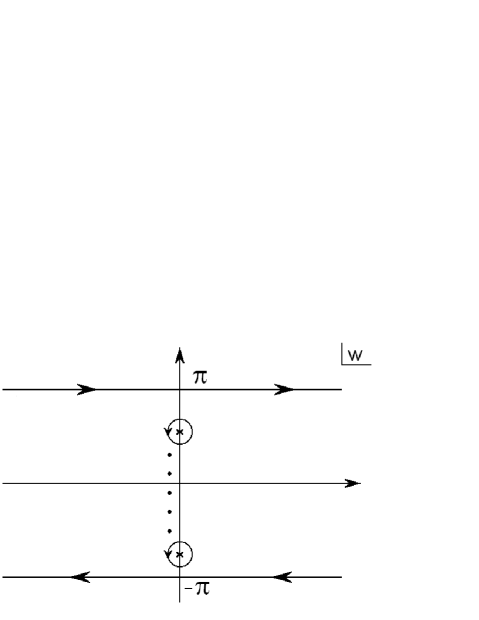
Figure 2: Two straight horizontal lines and circles enclosing simple poles at $w=-{\rm i}(\varphi+2\pi l)\nu^{-1}$ $(-\pi<{\rm Im}\,w<\pi)$.

where the summation is over integers $l$ satisfying condition

$$-\frac{\varphi}{2\pi}-\frac{\nu}{2}<l<-\frac{\varphi}{2\pi}+\frac{\nu}{2},$$ (A.9)

and contour $C_{=}$ consists of two straight horizontal lines depicted in figure 2. Substituting (A.8) into the last line of (A.5), we get

$$R^{\omega}(r,\varphi;\,r^{\prime},\varphi^{\prime})=\frac{1}{2\pi}\exp\left[{\rm i}\frac{e\Phi}{2\pi}(\varphi-\varphi^{\prime})\right]$$

$$\times\Biggl{[}\sum\limits_{l}e^{2{\rm i}lF\pi}K_{0}\left(\kappa\sqrt{(r-r^{\prime})^{2}+4rr^{\prime}\sin^{2}[(\varphi-\varphi^{\prime}+2\pi l)(2\nu)^{-1}])}\right)\Biggr{.}$$

$$\Biggl{.}-\frac{\nu}{2\pi{\rm i}}\int\limits_{C_{=}}{\rm d}w\,\frac{e^{(1-F)[\nu w+{\rm i}(\varphi-\varphi^{\prime})]}}{1-e^{\nu w+{\rm i}(\varphi-\varphi^{\prime})}}K_{0}\left(\kappa\sqrt{(r-r^{\prime})^{2}-4rr^{\prime}{\rm sinh}^{2}(w/2)}\right)\Biggr{]};$$ (A.10)

here the summation is over integers $l$ satisfying condition (15).

With the use of the resolvent kernel one can obtain Euclidean Green’s function in 2+1-dimensional space-time with the Wick-rotated time axis, $t=-{\rm i}\tau$:

$$G^{E}(\tau,\,r,\,\varphi;\,\tau^{\prime},\,r^{\prime},\,\varphi^{\prime})\equiv\langle\tau,\,r,\,\varphi|\left(-\partial^{2}_{\tau}-\Delta^{({\rm tr})}+m^{2}\right)^{-1}|\tau^{\prime},\,r^{\prime},\,\varphi^{\prime}\rangle$$

$$=\frac{1}{2\pi}\int\limits_{-\infty}^{\infty}{\rm d}p\,e^{{\rm i}p(\tau-\tau^{\prime})}R^{{\rm i}p}(r,\,\varphi;\,r^{\prime},\,\varphi^{\prime}).$$ (A.11)

Substituting (A.10) with $\omega={\rm i}p$ into the last line of (A.11) and performing the integration over $p$, we get

$$G^{E}(\tau,\,r,\,\varphi;\,\tau^{\prime},\,r^{\prime},\,\varphi^{\prime})=\frac{1}{2\pi^{2}}\exp\left[\frac{{\rm i}e\Phi}{2\pi}(\varphi-\varphi^{\prime})\right]$$

$$\times\left[\sum\limits_{l}e^{2{\rm i}lF\pi}\frac{\exp\left\{-m\sqrt{(\tau-\tau^{\prime})^{2}+(r-r^{\prime})^{2}+4rr^{\prime}\sin^{2}\left[(\varphi-\varphi^{\prime}+2\pi l)(2\nu)^{-1}\right]}\right\}}{\sqrt{(\tau-\tau^{\prime})^{2}+(r-r^{\prime})^{2}+4rr^{\prime}\sin^{2}\left[(\varphi-\varphi^{\prime}+2\pi l)(2\nu)^{-1}\right]}}\right.$$

$$\left.-\frac{\nu}{2\pi{\rm i}}\int\limits_{C_{=}}\!{\rm d}w\,\frac{e^{(1-F)[(\nu w+{\rm i}(\varphi-\varphi^{\prime})]}}{1-e^{\nu w+{\rm i}(\varphi-\varphi^{\prime})}}\frac{\exp\left[-m\sqrt{(\tau\!-\!\tau^{\prime})^{2}+(r\!-\!r^{\prime})^{2}\!-\!4rr^{\prime}{\rm sinh}^{2}(w/2)}\right]}{\sqrt{(\tau-\tau^{\prime})^{2}+(r-r^{\prime})^{2}-4rr^{\prime}{\rm sinh}^{2}(w/2)}}\right]\!.$$ (A.12)

Euclidean Green’s function in 3+1-dimensional space-time with imaginary time $t=-{\rm i}\tau$ can be obtained as a double Fourier transform of the resolvent kernel:

$$G^{E}(\tau,\,r,\,\varphi,\,z;\,\tau^{\prime},\,r^{\prime},\,\varphi^{\prime},\,z^{\prime})\equiv\langle\tau,\,r,\,\varphi,\,z|\left(-\partial_{\tau}^{2}-\Delta^{({\rm tr})}-\partial_{z}^{2}+m^{2}\right)^{-1}|\tau^{\prime},\,r^{\prime},\,\varphi^{\prime},z^{\prime}\rangle$$

$$=\frac{1}{(2\pi)^{2}}\int\limits_{-\infty}^{\infty}{\rm d}q\,e^{{\rm i}q(z-z^{\prime})}\int\limits_{-\infty}^{\infty}{\rm d}p\,e^{{\rm i}p(\tau-\tau^{\prime})}R^{{\rm i}\sqrt{q^{2}+p^{2}}}(r,\,\varphi;\,r^{\prime},\,\varphi^{\prime}),$$ (A.13)

or equivalently:

$$G^{E}(\tau,\,r,\,\varphi,\,z;\,\tau^{\prime},\,r^{\prime},\,\varphi^{\prime},\,z^{\prime})=\frac{1}{2\pi}\int\limits_{-\infty}^{\infty}{\rm d}q\,e^{{\rm i}q(z-z^{\prime})}G(\tau,\,r,\,\varphi;\,\tau^{\prime},\,r^{\prime},\,\varphi^{\prime})|_{m\rightarrow\sqrt{m^{2}+q^{2}}}.$$ (A.14)

Substituting (A.12) with $m\rightarrow\sqrt{m^{2}+q^{2}}$ into (A.14), we get

$$G^{E}(\tau,\,r,\,\varphi,\,z;\,\tau^{\prime},\,r^{\prime},\,\varphi^{\prime},\,z^{\prime})=\frac{m}{(2\pi)^{2}}\exp\left[\frac{{\rm i}e\Phi}{2\pi}(\varphi-\varphi^{\prime})\right]$$

$$\times\left[\sum\limits_{l}e^{2{\rm i}lF\pi}\frac{K_{1}\left(m\sqrt{(\tau-\tau^{\prime})^{2}+(r-r^{\prime})^{2}+(z-z^{\prime})^{2}+4rr^{\prime}\sin^{2}[(\varphi-\varphi^{\prime}+2\pi l)(2\nu)^{-1}]}\right)}{\sqrt{(\tau-\tau^{\prime})^{2}+(r-r^{\prime})^{2}+(z-z^{\prime})^{2}+4rr^{\prime}\sin^{2}\left[(\varphi-\varphi^{\prime}+2\pi l)(2\nu)^{-1}\right]}}-\right.$$

$$\left.-\frac{\nu}{2\pi{\rm i}}\int\limits_{C_{=}}{\rm d}w\,\frac{e^{(1-F)[\nu w+{\rm i}(\varphi-\varphi^{\prime})}}{1-e^{\nu w+{\rm i}(\varphi-\varphi^{\prime})}}\frac{K_{1}\left(m\sqrt{(\tau-\tau^{\prime})^{2}+(r-r^{\prime})^{2}+(z-z^{\prime})^{2}-4rr^{\prime}{\rm sinh}^{2}(w/2)}\right)}{\sqrt{(\tau-\tau^{\prime})+(r-r^{\prime})^{2}+(z-z^{\prime})^{2}-4rr^{\prime}{\rm sinh}^{2}(w/2)}}\right].$$

(A.15)

Proceeding in this way one can get Green’s function in space-time of arbitrary dimension, since

$$G^{E}(\tau,\,r,\,\varphi,\,z_{1},\,\ldots,\,z_{d-2};\,\tau^{\prime},\,r^{\prime},\,\varphi^{\prime},\,z_{1}^{\prime},\,\ldots,\,z_{d-2}^{\prime})$$

$$=\frac{1}{2\pi}\int\limits_{-\infty}^{\infty}{\rm d}q\,e^{{\rm i}q(z_{d-2}-z_{d-2}^{\prime})}G^{E}(\tau,\,r,\,\varphi,\,z_{1},\,\ldots,\,z_{d-3};\,\tau^{\prime},\,r^{\prime},\,\varphi^{\prime},\,z_{1}^{\prime},\,\ldots,\,z_{d-3}^{\prime})|_{m\rightarrow\sqrt{m^{2}+q^{2}}}.$$

(A.16)

The key point is the use of relation

$$\frac{1}{2\pi}\int\limits_{-\infty}^{\infty}{\rm d}q\,e^{{\rm i}qz}\frac{(q^{2}+m^{2})^{(d-2)/4}}{(2\pi a)^{(d-2)/2}}K_{(d-2)/2}(a\sqrt{q^{2}+m^{2}})=\left(\frac{m}{2\pi}\right)^{(d-1)/2}\frac{K_{(d-1)/2}\left(m\sqrt{a^{2}+z^{2}}\right)}{(a^{2}+z^{2})^{(d-1)/4}},$$

(A.17)

which is derived with the help of the integral representation for the Macdonald function (see, e.g., [53])

$$K_{\alpha}(2bc)=\frac{1}{2}\left(\frac{c}{b}\right)^{\alpha}\int\limits_{0}^{\infty}{\rm d}y\,y^{\alpha-1}\exp\left(-\frac{b^{2}}{y}-c^{2}y\right).$$

Thus, Euclidean Green’s function in $d+1$-dimensional space-time is given by expression

$$G^{E}\left(\tau,\,r,\,\varphi,\,{\bf z}_{d-2};\,\tau^{\prime},\,r^{\prime},\,\varphi^{\prime},\,{\bf z}_{d-2}^{\prime}\right)=\frac{m^{(d-1)/2}}{(2\pi)^{(d+1)/2}}\exp\left[\frac{{\rm i}e\Phi}{2\pi}(\varphi-\varphi^{\prime})\right]\left[\sum\limits_{l}e^{2{\rm i}lF\pi}\right.$$

$$\left.\times\frac{K_{(d-1)/2}\left(m\sqrt{(\tau-\tau^{\prime})^{2}+(r-r^{\prime})^{2}+({\bf z}_{d-2}-{\bf z}_{d-2})^{2}+4rr^{\prime}\sin^{2}[(\varphi-\varphi^{\prime}+2\pi l)(2\nu)^{-1}]}\right)}{\left\{(\tau-\tau^{\prime})^{2}+(r-r^{\prime})^{2}+({\bf z}_{d-2}-{\bf z}_{d-2}^{\prime})^{2}+4rr\sin^{2}[(\varphi-\varphi^{\prime}+2\pi l)(2\nu)^{-1}]\right\}^{(d-1)/4}}\right.$$

$$\left.-\frac{\nu}{2\pi{\rm i}}\int\limits_{C_{=}}{\rm d}w\,\frac{e^{(1-F)[\nu w+{\rm i}(\varphi-\varphi^{\prime})]}}{1-e^{\nu w+{\rm i}(\varphi-\varphi^{\prime})}}\right.$$

$$\left.\times\frac{K_{(d-1)/2}\left(m\sqrt{(\tau-\tau^{\prime})^{2}+(r-r^{\prime})^{2}+({\bf z}_{d-2}-{\bf z}_{d-2})^{2}-4rr^{\prime}{\rm sinh}^{2}(w/2)}\right)}{\left[(\tau-\tau^{\prime})^{2}+(r-r^{\prime})^{2}+({\bf z}_{d-2}-{\bf z}_{d-2})^{2}-4rr^{\prime}{\rm sinh}^{2}(w/2)\right]^{(d-1)/4}}\right].$$ (A.18)

Transforming the integral over contour $C_{=}$ into an integral over the real positive semiaxis, we get

$$G^{E}\left(\tau,\,r,\,\varphi,\,{\bf z}_{d-2};\,\tau^{\prime},\,r^{\prime},\,\varphi^{\prime},\,{\bf z}_{d-2}^{\prime}\right)=\frac{m^{(d-1)/2}}{(2\pi)^{(d+1)/2}}\exp\left[\frac{{\rm i}e\Phi}{2\pi}(\varphi-\varphi^{\prime})\right]\left[\sum\limits_{l}e^{2{\rm i}lF\pi}\right.$$

$$\left.\times\frac{K_{(d-1)/2}\left(m\sqrt{(\tau-\tau^{\prime})^{2}+(r-r^{\prime})^{2}+({\bf z}_{d-2}-{\bf z}_{d-2}^{\prime})^{2}+4rr^{\prime}\sin^{2}[(\varphi-\varphi^{\prime}+2\pi l)(2\nu)^{-1}]}\right)}{\left\{(\tau-\tau^{\prime})^{2}+(r-r^{\prime})^{2}+({\bf z}_{d-2}-{\bf z}_{d-2}^{\prime})^{2}+4rr^{\prime}\sin^{2}[(\varphi-\varphi^{\prime}+2\pi l)(2\nu)^{-1}]\right\}^{(d-1)/4}}\right.$$

$$\left.-\frac{\nu}{2\pi}\int\limits_{0}^{\infty}{\rm d}u\,\Omega_{\nu}^{F}(u,\,\varphi-\varphi^{\prime})\right.$$

$$\left.\times\frac{K_{(d-1)/2}\left(m\sqrt{(\tau-\tau^{\prime})^{2}+(r-r^{\prime})^{2}+({\bf z}_{d-2}-{\bf z}_{d-2}^{\prime})^{2}+4rr^{\prime}{\rm cosh}^{2}(u/2)}\right)}{\left[(\tau-\tau^{\prime})^{2}+(r-r^{\prime})^{2}+({\bf z}_{d-2}-{\bf z}_{d-2}^{\prime})^{2}+4rr^{\prime}{\rm cosh}^{2}(u/2)\right]^{(d-1)/4}}\right],$$ (A.19)

where $\Omega_{\nu}^{F}(u,\,\varphi)$ is given by (16). Going over to real time, we obtain Green’s function (14).

References

References

• [1] Abrikosov A A 1957 Sov. Phys. JETP 5 1174
• [2] Nielsen H B and Olesen P 1973 Nucl. Phys. B 61 45
• [3] Vilenkin A 1981 Phys. Rev. D 23 852
• [4] Gott III J R 1985 Astrophys. J. 288 422
• [5] Garfinkle D 1985 Phys. Rev. D 32 1323
• [6] Huebener R P 1979 Magnetic Flux Structure in Superconductors (Berlin: Springer-Verlag)
• [7] Vilenkin A and Shellard E P S 1994 Cosmic Strings and Other Topological Defects (Cambridge: Cambridge University Press)
• [8] Hindmarsh M B and Kibble T W B 1995 Rep. Prog. Phys. 58 477
• [9] Fraisse A A 2007 J. Cosmol. Astropart. Phys. JCAP 0703 008
• [10] Damour T and Vilenkin A 2005 Phys. Rev. D 71 063510
• [11] Brandenberger R, Firouzjahi H, Karoubi J and Khosravi S 2009 J. Cosmol. Astropart. Phys. JCAP 0901 008
• [12] Jackson M G and Siemens X 2009 J. High Energy Phys. JHEP 0906 089
• [13] Berezinsky V, Hnatyk B and Vilenkin A 2001 Phys. Rev. D 64 043004
• [14] Brandenberger R, Cai Y F, Xue W and Zhang X 2009 Preprint arXiv:0901.3474
• [15] Bevis N, Hindmarsh M, Kunz M and Urrestilla J 2008 Phys. Rev. Lett. B 100 021301
• [16] Pogosian L, Tye S-H H, Wasserman I and Wyman M 2009 J. Cosmol. Astropart. Phys. JCAP 0902 013
• [17] Davis A-C and Dimopoulos K 2005 Phys. Rev. D 72 043517
• [18] Gwyn R, Alexander S H, Brandenberger R H and Dasgupta K 2009 Phys. Rev. D 79 083502
• [19] Sitenko Yu A and Vlasii N D 2009 Class. Quantum Grav. 26 195009
• [20] Sarangi S and Tye S H H 2002 Phys. Lett. B 536 185
• [21] Jeannerot R, Rocher J and Sakellariadou 2003 Phys. Rev. D 68 103514
• [22] Polchinski J 2005 Int. J. Mod. Phys. A 20 3413
• [23] Davis A-C and Kibble T W B 2005 Contemporary Physics 46 313
• [24] Sakellariadou M 2009 Nucl. Phys. Proc. Suppl. 192-193 68
• [25] Copeland E J and Kibble T W B 2010 Proc. Roy. Soc. London A 466 623
• [26] Arkani-Hamed N, Dimopoulos S and Dvali G 1999 Phys. Rev. D 59 086004
• [27] Gherghetta T and Shaposhnikov M E 2000 Phys. Rev. Lett. 85 240
• [28] Lee H M and Papazoglou A 2006 Nucl. Phys. B 747 294
• [29] Bayntun A, Burgess C P and van Nierop L 2010 New J. Phys. 12 075015
• [30] Elvang H and Horowitz G T 2003 Phys. Rev. D 67 044015
• [31] Kastor D, Ray S and Traschen J H 2008 Class. Quantum Grav. 25 125004
• [32] Deutsch D and Candelas P 1979 Phys. Rev. D 20 3063
• [33] Helliwell T M and Konkowski D A 1986 Phys. Rev. D 34 1918
• [34] Linet B 1987 Phys. Rev. D 35 536
• [35] Frolov V P and Serebriany E M 1987 Phys. Rev. D 35 3779
• [36] Dowker J S 1987 Phys. Rev. D 36 3742
• [37] Guimaraes M E X and Linet B 1994 Commun. Math. Phys. 165 297
• [38] Moreira E S 1995 Nucl. Phys. B 451 365
• [39] Iellici D 1997 Class. Quantum Grav. 14 3287
• [40] Sitenko Yu A and Gorkavenko V M 2003 Phys. Rev. D 67 085015
• [41] Sitenko Yu A and Babansky A Yu 1998 Mod. Phys. Lett. A 13 379
• [42] Sitenko Yu A and Babansky A Yu 1998 Phys. At. Nucl. 61 1594
• [43] Sriramkumar L 2001 Class. Quantum Grav. 18 1015
• [44] Chernikov N A and Tagirov E A 1968 Ann. Inst. Henri Poincare, Sect. A 9 109
• [45] Callan C G, Coleman S and Jackiw R 1970 Ann. Phys. (N Y) 59 42
• [46] Fulling S A 1991 Aspects of Quantum Field Theory in Curved Space-Time (Cambridge: Cambridge University Press)
• [47] Geroch R and Traschen J H 1987 Phys. Rev. D 36 1017
• [48] Futamase T and Garfinkle D 1988 Phys. Rev. D 37 2086
• [49] Garfinkle D 1999 Class. Quantum Grav. 16 4101
• [50] Traschen J H 2009 Class. Quantum Grav. 26 075002
• [51] Israel W 1977 Phys. Rev. D 15 935
• [52] Sokolov D D and Starobinskii A A 1977 Sov. Phys. - Dokl. 22 312
• [53] Abramowitz M and Stegun I A (ed) 1972 Handbook of Mathematical Functions (New York: Dover)
• [54] Prudnikov A P, Brychkov Yu A and Marichev O I 1982 Integrals and Series: Elementary Functions (New York: Gordon & Breach)
• [55] Aharonov Y and Bohm D 1959 Phys. Rev. 115 485
• [56] ’t Hooft G 1988 Commun. Math. Phys. 117 685
• [57] Deser S and Jackiw R 1988 Commun. Math. Phys. 118 495
• [58] de Sousa Gerbert P and Jackiw R 1989 Commun. Math. Phys. 124 229
• [59] Sitenko Yu A and Mishchenko A V 1995 J. Exp. Theor. Phys. (JETP) 81 831
• [60] Sitenko Yu A and Vlasii N D 2010 J. Phys. A: Math. Theor. 43 354014