A $K_{S}$ and IRAC Selection of High-Redshift Extremely Red Objects

Abstract

In order to find the most extreme dust-hidden high-redshift galaxies, we select 196 extremely red objects in the $K_{S}$ and IRAC bands (KIEROs, $[K_{s}-4.5\mu\rm m]_{\rm AB}>1.6$) in the 0.06 deg² GOODS-N region. This selection avoids the Balmer breaks of galactic spectra at $z<4$ and picks up red galaxies with strong dust extinction. The photometric redshifts of KIEROs are between 1.5 and 5, with $\sim 70\%$ at $z\sim 2$–4. KIEROs are very massive, with $M_{\star}\sim 10^{10}$–$10^{12}M_{\sun}$. They are optically faint and usually cannot be picked out by the Lyman break selection. On the other hand, the KIERO selection includes approximately half of the known millimeter and submillimeter galaxies in the GOODS-N. Stacking analyses in the radio, millimeter, and submillimeter all show that KIEROs are much more luminous than average 4.5 $\mu$m selected galaxies. Interestingly, the stacked fluxes for ACS-undetected KIEROs in these wavebands are 2.5–5 times larger than those for ACS-detected KIEROs. With the stacked radio fluxes and the local radio–FIR correlation, we derive mean infrared luminosities of 2–$7\times 10^{12}L_{\sun}$ and mean star formation rates of 300-1200 $M_{\sun}$ yr^-1 for KIEROs with redshifts. We do not find evidence of a significant subpopulation of passive KIEROs. The large stellar masses and star formation rates imply that KIEROs are $z>2$ massive galaxies in rapid formation. Our results show that a large sample of dusty ultraluminous sources can be selected in this way and that a large fraction of high-redshift star formation is hidden by dust.

1. Introduction

Deep imaging in the submillimeter opened a new window for studying high-redshift galaxies (Smail, Ivison, & Blain, 1997; Hughes et al., 1998; Barger et al., 1998). The brighter submillimeter galaxies (SMGs, typical total infrared luminosity greater than $10^{13}L_{\sun}$) that have radio counterparts were found to be at redshifts mostly between 2 and 3 (Chapman et al., 2003, 2005). Despite the extremely large star formation rates (SFRs), typically $>1000$ $M_{\sun}$ yr^-1, such galaxies do not emit strongly in the rest-frame ultraviolet (UV) and therefore are generally not Lyman break galaxies (LBGs; Peacock et al., 2000; Chapman et al., 2000; Webb et al., 2003). (A counter example is a $z=4.55$ SMG in Capak et al., 2008, which was originally selected as an LBG.) This implies a large fraction of dusty star formation at high redshift being missed by rest-frame UV surveys.

This raises two general questions: will we start to see galaxies similar to optically selected ones if we are able to probe deeper in the submillimeter, and exactly how much high-redshift star formation is missed by optical surveys? We are not close to being able to answer either question. Deep submillimeter surveys in lensing clusters are able to probe dusty galaxies with IR luminosities $\lesssim 10^{12}L_{\sun}$ and constrain their number density (Blain et al., 1999; Cowie, Barger, & Kneib, 2002; Knudsen, van der Werf, & Kneib, 2008; Chen et al., 2011), but the identification of their optical counterparts is not yet complete, and the sample sizes are very small. Furthermore, a $z\gtrsim 4$ SMG, GOODS 850-5, was recently found to be extremely faint in the optical and near-infrared (NIR) at $\lambda_{\rm obs}<2.2$ $\mu$m (Wang et al., 2007; Wang, Barger, & Cowie, 2009). If a significant fraction of the $z>2$ SMGs in the IR luminosity range $10^{12}$–$10^{13}$ $L_{\sun}$ are like GOODS 850-5, then identifying them in the radio and optical will be challenging even with next-generation instruments. We therefore seek a NIR diagnosis of extremely optically faint SMGs. A general description of the Spitzer Infrared Array Camera (IRAC) colors of bright SMGs was recently developed by Yun et al. (2008). Here we focus on the reddest galaxies in the IRAC and $K_{S}$ bands.

In this paper we present a new color selection of extremely red objects (EROs) with $K_{S}$ and IRAC colors of $K_{S}-4.5$ $\mu$m $>1.6$. We refer to such sources as KIEROs. This selection is motivated by the fact that at least half of known SMGs are redder than this color (Section 2). Among all existing ERO selections, the KIERO selection utilizes the longest wavebands that are practically accessible for deep imaging. Unlike some other selections for high-redshift red objects, the KIERO selection does not particularly aim at the 4000 Å Balmer breaks in galactic spectra, which only enter the $K_{S}$ band at $z\sim 4$. Instead, this selection aims at galaxies at $z>2$ whose extremely red colors are likely caused by large dust extinction (Section 4). Also because of this, we choose the 4.5 $\mu$m band instead of the 3.6 $\mu$m band, to be more sensitive to galaxies whose spectral energy distributions (SEDs) are red over a broad wavelength range (cf. sharp spectral breaks).

The paper is organized as following. We describe the data and the KIERO selection in Section 2, the number counts in Section 3, the optical and NIR SEDs, redshift distribution, and stellar populations in Section 4, and the radio, millimeter, submillimeter, and X-ray properties in Section 5. We identify active galactic nuclei (AGNs) in KIEROs in Section 6. We estimate the SFRs and SFR densities (SFRDs) of KIEROs in Section 7. We compare KIEROs with other high-redshift galaxy populations in Section 8. We discuss the roles of KIEROs in galaxy formation in Section 9 and summarize our results in Section 10. Throughout the paper, we assume cosmological parameters of $H_{0}=71$ km s^-1 Mpc^-1, $\Omega_{M}=0.27$, and $\Omega_{\Lambda}=0.73$. All magnitudes are in the AB system, where an AB magnitude is defined as $\rm AB=8.9-2.5\log(\rm fluxinJy)$.

2. The KIERO Sample

We use our publicly released $K_{S}$ and IRAC catalogs (Wang et al., 2010, hereafter W10) of the Great Observatories Origins Deep Surveys-North (GOODS-N; Giavalisco et al., 2004) field. The $K_{S}$ source catalog of W10 is extracted from an extremely deep Canada-France-Hawaii Telescope $K_{S}$ image, which has a $1\sigma$ depth of 0.12 $\mu$Jy in the GOODS-N region. W10 used the GOODS-N Spitzer IRAC images at 3.6–8.0 $\mu$m (M. Dickinson et al. 2011, in preparation) to measure the IRAC photometry of the $K_{S}$ selected sources using a CLEAN-like method that takes the $K_{S}$ catalog and image as priors. W10’s primary $K_{S}$ and IRAC catalog contains 15018 $K_{S}$ selected sources that are detected at 3.6 and 4.5 $\mu$m in the GOODS-N region. W10’s secondary catalog contains 358 $K_{S}$-faint IRAC detected sources.

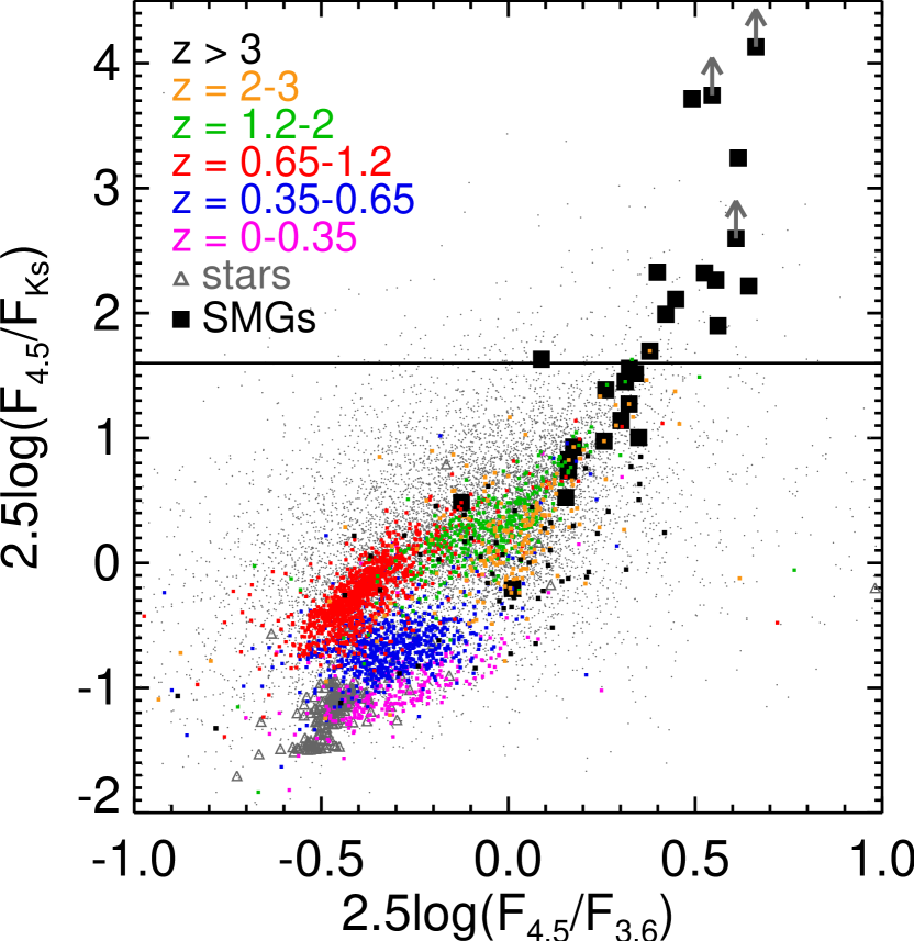
Figure 1.— $K_{S}$, 3.6 $\mu$m, and 4.5 $\mu$m color–color diagram. Small gray dots are 3 $\sigma$ 4.5 $\mu$m sources in the catalog of W10. Spectroscopically identified sources in Barger, Cowie, & Wang (2008), including stars, are shown with color symbols. Radio and submillimeter interferometrically identified 4 $\sigma$ SMGs in the sample of Wang et al. (2004) and Perera et al. (2008) are shown with filled squares. The horizontal line indicates our selection criterion for KIEROs.

We show the $K_{S}$, 3.6 $\mu$m, and 4.5 $\mu$m color–color diagram for sources with $>3\sigma$ 4.5 $\mu$m fluxes in W10’s primary catalog in Figure 1. To obtain colors of GOODS-N SMGs, we looked for $K_{S}$ and IRAC counterparts of the SMGs in the 4 $\sigma$ SCUBA sample of Wang, Cowie, & Barger (2004) and AzTEC sample of Perera et al. (2008). We only include SMGs with unambiguous radio interferometric identifications (Wang et al. 2004; Pope et al., 2006; Chapin et al., 2009) or submillimeter interferometric identifications (Iono et al., 2006; Wang et al., 2007; Daddi et al., 2009a; Wang et al., 2011; A. J. Barger et al. 2011, in preparation). There are 28 such SMGs and they are shown with squares in Figure 1. Fourteen of them are redder than $K_{S}-4.5\mu\rm{m}=1.6$ (horizontal line in the figure) and three are not even detected in $K_{S}$ (lower limits in the figure). They occupy a color space significantly different than that of most sources detected at both $K_{S}$ and 4.5 $\mu$m. Because most spectroscopically identified SMGs are at $z<3$ (Chapman et al., 2003, 2005), the extremely red colors of these SMGs must be caused by very high redshifts and/or extremely large dust extinctions (see Section 4), like in the case of GOODS 850-5 (Wang et al., 2007; Wang, Barger, & Cowie, 2009). Such extremely red SMGs are of particular interest. Since it is known that a variety of optical/NIR criteria are required to include all bright SMGs (Reddy et al., 2005), here we only focus on selecting and understanding the extremely red ones.

In order to find sources similar to the extremely red SMGs but slightly fainter in the submillimeter and therefore undetected by current submillimeter surveys, we select KIEROs with $K_{S}-4.5$ $\mu$m $>1.6$. We require that the sources be detected at $>3\sigma$ in the 4.5 $\mu$m band and in at least one other IRAC band. For galaxies detected in the IRAC bands but not in the $K_{S}$ band (in W10’s secondary catalog), we adopt their $1\sigma$ $K_{S}$ limits. Although W10’s primary catalog is a $K_{S}$ selected one, the above inclusion of $K_{S}$-faint 4.5 $\mu$m sources in W10’s secondary catalog makes the selection of KIEROs in principle a 4.5 $\mu$m selection. We visually inspected the IRAC images of all such galaxies and excluded those whose IRAC fluxes are less reliable, mainly galaxies affected by very bright stars in the field and galaxies blended with $\geq 3$ bright nearby galaxies. These are the limitations of W10’s catalogs (see W10 for discussion). This reduces the number of selected KIEROs by $<10\%$ and should not impact our analyses, even if some of them are truly red sources. We are left with 104 KIEROs in the main $K_{S}$-selected sample and 92 in the $K_{S}$ undetected sample. Among the above mentioned 28 identified SMGs in the GOODS-N, 14 are KIEROs.

3. Number Counts

Figure 2 shows a $K_{S}$ and 4.5 $\mu$m color–magnitude diagram for KIEROs and field galaxies. The KIEROs are a relatively rare population among all sources detected at 4.5 $\mu$m, and the selection of KIEROs lies very close to the detection limits at both $K_{S}$ and 4.5 $\mu$m. At $K_{S}$, W10 provided a description of the completeness limits (e.g., the $K_{S}$ 30% limit shown by the diagonal dashed line in Figure 2). On the other hand, it is nontrivial to quantify the completeness at 4.5 $\mu$m, which depends on both the $K_{S}$ completeness and the very complex procedures used by W10 to construct the 4.5 $\mu$m source lists.

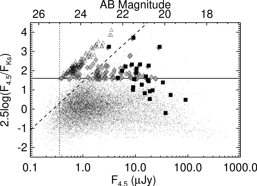
Figure 2.— $K_{S}$ and 4.5 $\mu$m color–magnitude diagram. Dots are field galaxies detected (3$\sigma$) in both the $K_{S}$ and 4.5 $\mu$m bands, as well as at least one other IRAC band. Diamonds are $K_{S}$ detected KIEROs, and triangles are $1\sigma$ color lower limits of $K_{S}$ undetected KIEROs. Squares are the radio and submillimeter interfeormetrically identified SMGs. The horizontal solid line shows the selection criterion for KIEROs. Some of the galaxies above the horizontal line are not designated as KIEROs because their 4.5 $\mu$m fluxes in W10’s catalogs are less reliable, mostly bad photometry affected by very bright stars in the field or galaxies blended with $\geq 3$ bright nearby galaxies. The diagonal dashed line shows the $K_{S}$ 30% completeness limit determined by W10. The vertical dotted line shows the $3\sigma$ limit of the 4.5 $\mu$m fluxes from W10. The completeness at 4.5 $\mu$m is unclear due to the nature of the 4.5 $\mu$m catalog (see W10 for details).

Figure 3.— $K_{S}$ number counts of KIEROs. The solid histogram shows the number of sources detected in the $K_{S}$ band at $>3\sigma$ in bins of 0.2 dex in flux. The dashed histogram shows the same for sources with only $K_{S}$ upper limits ($1\sigma$). The vertical dotted lines are the 90% and 30% completeness limits of the WIRCam $K_{S}$ image derived by W10. The actual completeness of the $K_{S}-4.5$ $\mu$m selection should be even lower (see text). The number distributions shown here are not corrected for completeness.

Because of the above issues, we have decided to present the $K_{S}$ number counts of KIEROs (Figure 3), even though this is a 4.5 $\mu$m selected population. In our survey there are no KIEROs brighter than 6 $\mu$Jy at $K_{S}$. The raw counts slightly flatten at $\sim 1$ $\mu$Jy and drop rapidly below 0.3 $\mu$Jy, consistent with the $K_{S}$ detection completeness. Without considering the completeness at 4.5 $\mu$m, simply correcting the counts with the $K_{S}$ completeness derived by W10 suggests that the slope of the counts does not change significantly down to a flux level of $\sim 0.3$ $\mu$Jy. A slope of $0.41\pm 0.07$ in the logN-mag space was fitted at $F_{Ks}>0.3$ $\mu$Jy using completeness corrected counts weighted by the Poisson errors. Comparing to the slope for the entire $K_{S}$ sample in the same flux range ($\sim 0.2$, e.g., Maihara et al., 2001; Keenan et al., 2010), this is much steeper. This is likely a consequence of the higher redshifts of KIEROs (see next section). Furthermore, the large number of $K_{S}$-undetected sources that meet our KIERO selection criterion (dashed histogram in Figure 3) suggests that the counts may be still rising at a $K_{S}$ flux of $\sim 0.2$ $\mu$Jy.

4. Redshift and Stellar Population

To obtain a rough idea about the SEDs and redshifts of KIEROs, we plot the color–redshift diagram of spectroscopically identified 4.5 $\mu$m sources in Figure 4. Most 4.5 $\mu$m sources have $K_{S}-4.5$ $\mu$m colors bluer than 1.0. Even AGNs, which tend to have unusual colors, are mostly bluer than 1.0. In general, we only expect heavily extinguished ($A_{V}>2$) galaxies at $z>2$ to be redder than 1.6. At $z<2$, galaxies can be redder than 1.6 in only the most extreme cases. We do not expect to see many such galaxies. To verify that KIEROs are mostly at $z>2$, we looked at the spectroscopic redshifts of GOODS-N galaxies and carried out a photometric redshift analysis.

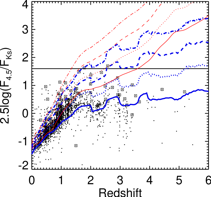
Figure 4.— $K_{S}$-4.5 $\mu$m color vs. spectroscopic redshifts. Dots are 3$\sigma$ 4.5 $\mu$m sources in the catalog of W10 that are spectroscopically identified in Barger et al. (2008). Squares show X-ray selected AGNs (soft or hard X-ray luminosities greater than $10^{42}$ erg s^-1). Curves show colors derived from the models of elliptical galaxies (thin red curves, Coleman, Wu, & Weedman, 1980) and starburst galaxies (thick blue curves, Kinney et al., 1996), reddened with the Calzetti et al. (2000) extinction law with $A_{V}=0$ (solid), 1.0 (dotted), 2.0 (dashed), and 3.0 (dash-dotted).

4.1. Spectroscopic Redshift

In the entire KIERO sample, only two sources are bright enough in the optical and NIR to have spectroscopic redshifts in our redshift survey (Barger, Cowie, & Wang, 2008). Both are detected in the 2 Ms Chandra image (source numbers 109 and 135 in the catalog of Alexander et al., 2003). One is the SMG GOODS 850-7 ($F_{1.4~{}\rm GHz}=58$ $\mu$Jy, $F_{850~{}\rm\mu m}=6.2$ mJy) at $z=2.578$. The other is a $F_{1.4~{}\rm GHz}=83$ $\mu$Jy radio source at $z=1.790$. This radio source is very close to the bright SMG GOODS 850-2 ($F_{850~{}\rm\mu m}=10.3$ mJy), with an angular separation of $\sim 8\farcs 6$ based on its SCUBA position (Wang et al. 2004; see also Barger, Cowie, & Richards, 2000). However, our recent submillimeter interferometric observation (A. J. Barger et al., in preparation) shows that GOODS 850-2 is another faint $K_{S}$-band source that also enters our KIERO sample.

In addition to the two optical spectroscopic redshifts, an SMG KIERO, GOODS 850-5 (Wang et al., 2007), has a plausible millimeter spectroscopic redshift of 4.042 based on a line detection at 91.4 GHz that is likely a CO(4–3) transition (Daddi et al., 2009b). The three spectroscopic redshifts span a redshift range that agrees with what would be expected based on Figure 4. However, the sample size is too small and we need to rely on photometric redshift fitting.

4.2. Photometric Redshift

We carried out a photometric redshift analysis on a subsample of 76 high S/N KIEROs whose ${K_{S}}$ fluxes are greater than 0.2 $\mu$Jy. We included the photometry in the $U$, HST ACS, $J$, WFC3 F140W, $K_{S}$, and IRAC bands. We adopted the $U$-band fluxes from Capak et al. (2004). For the ACS bands, we directly adopted the fluxes from the GOODS-N v2 catalog (Giavalisco et al., 2004). We measured $J$-band fluxes from a CFHT WIRCam image that contains $\sim 27$ hr of total integration. We obtained the $J$-band images from the public archive. They were originally obtained by a Taiwanese team led by Lihwai Lin (2010, in preparation). We reduced and processed the $J$-band images in an identical manner to W10 for the $K_{S}$-band images. The HST WFC3 F140W data will be described by A. Barger et al. (2011, in prep).

For photometric redshift fitting, we tried two packages: the latest version of Hyperz (Bolzonella, Miralles, & Pelló, 2000), and EAZY (Brammer, van Dokkum, & Coppi, 2008). We found that EAZY generally produces better results and includes a necessary feature for our studies (see below). Our primary photometric redshift results in this paper are thus based on EAZY. We adopted the default set of SED templates of Blanton & Roweis (2007), provided in the EAZY package. This set includes five templates ranging from very blue and young galaxies with strong emission lines, to galaxies dominated by old stars. We included an additional SMG-type dusty starburst model ($t=50$ Myr, $A_{V}=2.75$), also provided in the EAZY package. We refer to Brammer et al. (2008) for detailed descriptions on all these SED models. The templates here all already include certain amounts of extinction in order to fit galaxy SEDs in deep surveys. To account for very dusty sources in the KIERO sample, we further reddened these templates (including the already reddened SMG template) by $A_{V}=0$, 0.5, and 1.0 with the extinction law of Calzetti et al. (2000). To account for the situation where there are more than two distinct stellar populations in a galaxy, we allowed for all linear combinations of the templates in the fitting. In Section 4.3 we will show that the EAZY feature of allowing for all linear combinations of templates is essential. Because a fitted SED is a combination of multiple templates, we are not able to quote an extinction value for a source. In Figure 5(a) we show the distribution of the EAZY photometric redshifts.

Figure 5.— Results of photometric redshifts for $F_{Ks}>0.2$ $\mu$Jy sources in the KIERO sample. A total of 76 KIEROs are included. The top panel shows the distribution of the EAZY photometric redshifts. The bottom panel shows the stellar masses fitted by Hyperz at the EAZY redshifts using the models of Bruzual & Charlot (2003) (see Section 4.3). The vertical bars show the maximum and minimum stellar masses from various types of models, while the squares are the best-fit masses. Large open squares denote AGNs identified in Section 6, which may have problematic photometric redshifts and masses.

In order to see how reliable the fitting is, we ran EAZY on $\sim 1500$ $F_{Ks}>0.2$ $\mu$Jy galaxies in the spectroscopic sample of Barger et al. (2008). The results are shown in Figure 6. If we define $\Delta z$ as $(z_{\rm ph}-z_{\rm sp})/(1+z_{\rm sp})$, then only 5.3% of the galaxies have $|\Delta z|>0.2$. After excluding these outliers, there is an rms dispersion of 0.05 and a median systematic offset of -0.01 in $\Delta z$. We also made the same comparison on Hyperz results. The outlier fraction and dispersion in $\Delta z$ are both significantly worse than the EAZY ones.

Figure 6.— Results of EAZY photometric redshifts for the $F_{Ks}>0.2$ $\mu$Jy sources (small dots) in the spectroscopic sample of Barger et al. (2008). A total of 1987 galaxies are included. Large squares are the two KIEROs with spectroscopic redshifts.

Although the results in Figure 6 look good, there is no guarantee that we can achieve the same on KIEROs. The two KIEROs with spectroscopic redshifts at $z=2.578$ and 1.790 have EAZY photometric redshifts of 2.03 and 1.96, respectively (large squares in Figure 6). These are excellent, but the sample is too small for us to comment on the overall quality. We can also compare the photometric redshifts on KIEROs that show continuum dropouts (Lyman breaks, see also Section 8.3). There are 15 $b$-dropouts in the KIERO sample, 6 of which are bright enough at $K_{S}$ to have photometric redshifts. Their mean photometric redshift is $3.72\pm 0.50$. There are 4 $v$-dropouts in the KIERO sample, 2 of which have photometric redshifts of 5.02 and 4.71. These are all consistent with the expected redshifts for the dropouts (e.g., Bouwens et al., 2007). Finally, Figure 7 shows that the majority of the fitted SEDs reasonably represent the observed SEDs, including various spectral breaks (the Lyman breaks, Balmer breaks, and 1.6 $\mu$m bumps), except AGNs (Section 6) with featureless power-law SEDs in the IRAC bands. It is worth noting that there are three non-AGN data points at $z>4$ with unusually large stellar masses (Section 4.3) of $\sim 10^{12}M_{\sun}$. They are #23, 24, and 38 in Figure 7. Their observed SEDs are also quite featureless in the IRAC bands, and all fade dramatically at $K_{S}$ and shorter wavebands, likely because of extinction. Although they are not identified as AGNs, we suspect that their photometric fittings are unreliable. Except for AGNs and these few problematic cases, the EAZY photometric redshifts for the majority of the sources seem reasonably good. In Section 5.2 we present independent evidence suggesting that the redshift distribution in Figure 5(a) is approximately correct.

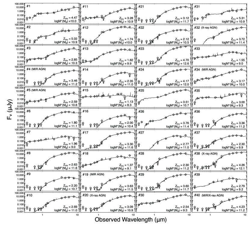
Figure 7.— Observed (diamonds) and fitted (curves) SEDs in the EAZY photometric redshift analysis. Sources without symbols in the ACS and F140W bands are outside the image region. Sources without symbols in the $J$ band do not have reliable $J$-band counterpart identifications. AGNs identified in Section 6 are indicated in the upper-left corners and have problematic photometric redshifts.

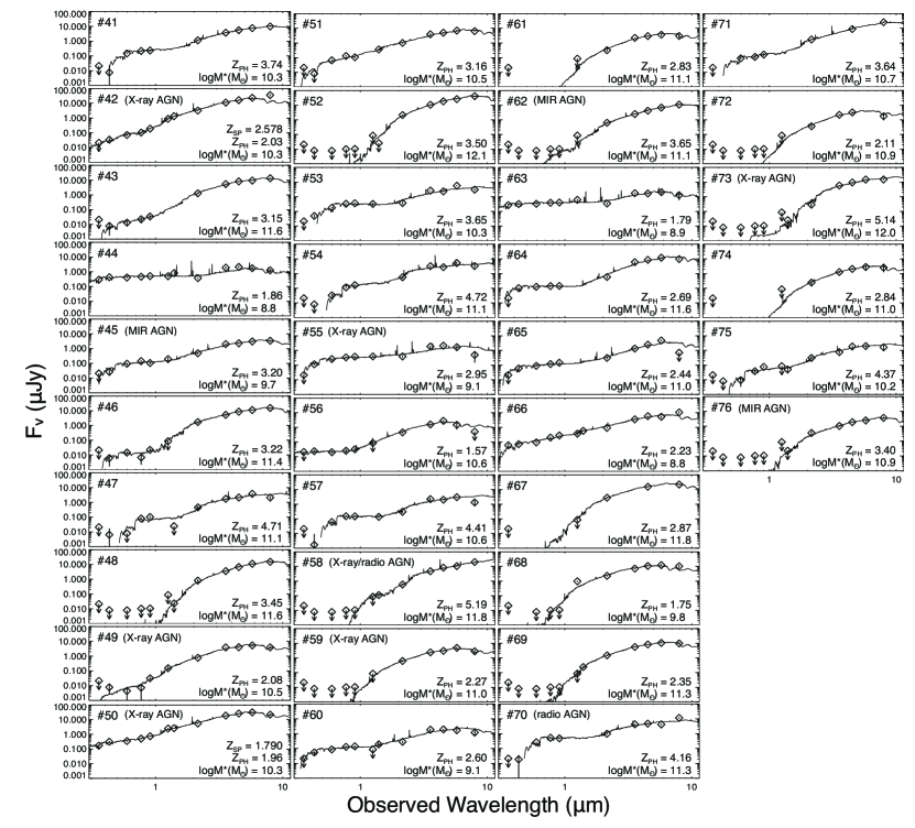
Figure 7.— Continued.

We did not attempt to study the redshifts of fainter sources ($F_{Ks}<0.2$ $\mu$Jy). Such sources often have robust photometry in only two IRAC bands, which is insufficient for good photometric redshifts. One might expect that these fainter sources should have higher redshifts rather than lower intrinsic luminosities. However, we cannot test this with the current data.

4.3. Stellar Population

When testing the photometric redshift fitting, we found that many KIEROs have SEDs that cannot be fitted with a single stellar population by Hyperz. For example, on the above mentioned six $b$-dropouts, Hyperz returns a mean redshift of $2.98\pm 0.34$. This is clearly too low, a consequence of trying to fit the complex SEDs with single stellar populations. This is a key reason for our adoption of EAZY, which allows for combinations of different SED templates. The most obvious cases of such KIEROs are sources 3, 11, 30, 35, 41, 53, and 70 in Figure 7. In such KIEROs, there are well-evolved old stellar populations, which produce the observed NIR luminosity, as well as unobscured ongoing star formation, which produces the strong rest-frame UV emission. This property is similar to that of objects selected with $z-3.6~{}\mu\rm m>3.25$ (IEROs) by Yan et al. (2004) in the Hubble Ultra Deep Field (HUDF; Beckwith et al., 2006). Interestingly, our stacking analyses in the radio and FIR (Section 5 and Table 1) show that sources that are faint in the rest-frame UV have more intensive starbursts. SFR estimates based on rest-frame UV may miss the strong dust-hidden star formation on such optically faint sources.

Another interesting question to ask is whether or not KIEROs are massive galaxies. Unfortunately, EAZY does not provide direct estimates of stellar masses. To do this, we rely on Hyperz, which builds in the stellar population synthesis models of Bruzual & Charlot (2003) and provides stellar mass estimates. We forced Hyperz to fit at the EAZY redshifts. We derived two sets of stellar masses by fitting to the full SEDs of the KIEROs, and by fitting to just the infrared SEDs in the $J$ and redder bands. We found that neither of the two masses systematically favor high or low mass values. For roughly 2/3 of the objects, these two masses agree within 0.4 dex. We thus believe that for most of the objects, the derived masses are robust. On the other hand, since many of the KIEROs show two different stellar populations, it is better to just fit the rest-frame NIR parts of the SEDs. The mass-to-light ratios in the NIR are relatively insensitive to both extinction and ongoing star formation. Nevertheless, we remind the reader that our mass estimates are significantly limited by the fact that Hyperz can only fit the SEDs with single stellar populations.

In Figure 5(b) we show the best fit stellar masses (squares) and the maximum and minimum masses (vertical bars) from the various templates of Bruzual & Charlot (2003), based on just fitting the infrared SEDs. For most KIEROs, the data only allow small ranges of stellar masses, a consequence of similar mass-to-light ratios in the NIR. They have large stellar masses of $10^{10}M_{\sun}$ to $\gtrsim 10^{12}M_{\sun}$. Some of the masses seem unusually large, especially at the high-redshift end ($z>4$) where less photometric data points are available and there is a degeneracy between photometric redshift, age, and extinction. This is a fundamental limit of the current data. We also note that there are 18 sources with stellar masses less than $10^{10}M_{\sun}$, giving a mass distribution that is somewhat disjoint from that of the other KIEROs. These are all optically bright sources with $F_{\rm F850LP}>0.2$ $\mu$Jy and have lower redshifts. They are likely a less dusty subclass of KIEROs.

In summary, the majority of KIEROs in the photometric redshift subsample are more massive than $10^{10}M_{\sun}$. In addition to the massive stellar populations, a large fraction of KIEROs show young stellar populations in the rest-frame UV. In the following sections of this paper, we will focus on the star formation properties of KIEROs.

5. Multiwavelength Properties and Stacking Analyses

5.1. Radio Properties

In order to understand the star formation activities in KIEROs (albeit with AGN contamination), we studied their radio properties. We used the Very Large Array (VLA) 1.4 GHz image and catalog in the Hubble Deep Field-North (HDF-N) published by Morrison et al. (2010). The image has a 5 $\sigma$ sensitivity of 20 $\mu$Jy at the field center, and the catalog contains $\sim 430$ sources in the GOODS-N region. Among the 196 KIEROs, 22 are included in the catalog of Morrison et al. (2010).

For sources not in the catalog of Morrison et al. (2010), we measured their fluxes from the image with $3\arcsec$ apertures after correcting for the VLA primary beam and the band-width smearing. We compared our fluxes on compact sources with those in the catalog of Morrison et al. (2010), and they are fully consistent with each other. The adopted aperture size is $2\times$ the VLA beam FWHM and corresponds to 20–25 kpc at $z=2$–5. This size is slightly less optimized for detecting faint and compact sources, but it encloses most of the radio flux if the radio-emitting region in a high-redshift galaxy is offset from the position determined by NIR observations by a few kpc. Such offsets are not uncommon in nearby interacting/merging systems. The measured 1.4 GHz fluxes of the KIEROs are shown in the bottom and middle panels of Figure 8.

Figure 8.— Radio flux vs. 4.5 $\mu$m flux for KIEROs. The bottom and middle panels show the radio fluxes of individual sources. The middle panel is a blowup of the bottom panel. Sources in the bottom and middle panels enclosed in large squares are AGNs identified in Section 6. The top panel shows the stacked radio fluxes in each 0.5 dex 4.5 $\mu$m flux bin. Solid squares are the mean fluxes after excluding the $F_{1.4~{}\rm GHz}>600$ $\mu$Jy bright source. The exact values are also shown near the symbols. Open squares are the median fluxes, which further avoid influence from $>200$ $\mu$Jy sources. Triangles show the mean fluxes of the entire 4.5 $\mu$m sample in the same flux ranges. The dotted line corresponds to roughly $5\sigma$. Stacking of faint sources below this line is presented in the lower half of Table 1.

We can study the mean 1.4 GHz fluxes of KIEROs via a “stacking analysis,” in which we measure radio fluxes with $3\arcsec$ apertures at the locations of KIEROs and average the results. First, we need to understand the bias and uncertainty in such stacked fluxes, for which we took a Monte Carlo approach. We randomly placed $3\arcsec$ apertures in the VLA image, calculated their mean flux, and repeated a large number of such measurements. The mean flux measured in this way is an estimate of contamination from physically unrelated nearby sources. We refer to this as confusion. We excluded flux values greater than 600 $\mu$Jy to avoid being biased by the very bright source, which is likely an AGN (also see Section 5.3). In the IRAC region, the mean 1.4 GHz flux is 0.41 $\mu$Jy for the random positions in the Monte Carlo simulations. We subtracted this value from the mean flux of each KIERO sample.

We treated the dispersion between various measurements of the mean flux of random apertures as noise in the mean, which has contributions from the receiver noise and from the confusion noise. We varied the number of random apertures that we placed in the image each time, and we found that even with source densities up to $10^{6}$ deg^-2, the measured noise in the mean precisely scales with the square-root of the source number. In the IRAC region, such noise is 8.7 $\mu$Jy per source. This value is larger than the nominal 4 $\mu$Jy noise of the image, a consequence of confusion caused by bright sources. On the other hand, the average fluxes we determine are considerably below the conventional single-source detection limit.

We present our major stacking analysis results in Table 1. For the entire sample of 196 KIEROs, excluding the $>600$ $\mu$Jy one, the mean 1.4 GHz flux is $9.9\pm 0.6$ $\mu$Jy, and the median is 3.07 $\mu$Jy. For comparison, in the 4.5 $\mu$m sample there are 8977 sources with $F_{4.5~{}\rm\mu m}>1$ $\mu$Jy. Their mean 1.4 GHz flux is $4.7\pm 0.1$ $\mu$Jy, and their median flux is 2.46 $\mu$Jy. After considering the fact that most of the 4.5 $\mu$m sources are at $z<2$ while most of the KIEROs are at $z>2$, it is clear that our $K_{S}-4.5$ $\mu$m $>1.6$ selection picks up a much more radio luminous population.

Table 1Stacking Results in the Radio, Millimeter, and Submillimeter

Samples	1.4 GHz Stacking (0.06 deg2)				1100 $\mu$m Stacking (0.06 deg2)				850 $\mu$m Stacking (0.028 deg2)
	$N$	$\langle F\rangle$	EBL		$N$	$\langle F\rangle$	EBL		$N$	$\langle F\rangle$	EBL
		($\mu$Jy)	(mJy deg-2)			(mJy)	(Jy deg-2)			(mJy)	(Jy deg-2)
$F_{4.5~{}\rm\mu m}>1$ $\mu$Jy	8977	$4.7\pm 0.1$	$706\pm 15$		8984	$0.090\pm 0.01$	$13.4\pm 1.8$		4551	$0.14\pm 0.04$	$22.7\pm 6.4$
KIERO	195	$9.9\pm 0.6$	$32.2\pm 2.0$		196	$0.50\pm 0.08$	$1.64\pm 0.26$		87	$1.44\pm 0.28$	$4.47\pm 0.88$
KIERO, $z<3.0$	38	$22.7\pm 1.4$	$14.4\pm 0.9$		38	$0.56\pm 0.18$	$0.36\pm 0.12$		18	$2.48\pm 0.62$	$1.59\pm 0.40$
KIERO, $z>3.0$	37	$21.0\pm 1.4$	$12.9\pm 0.9$		38	$1.57\pm 0.18$	$1.00\pm 0.12$		14	$3.19\pm 0.71$	$1.59\pm 0.35$
KIERO, ACS	112	$6.0\pm 1.0$	$11.2\pm 1.5$		112	$0.23\pm 0.11$	$0.42\pm 0.20$		52	$0.71\pm 0.37$	$1.32\pm 0.68$
KIERO, non-ACS	61	$16.2\pm 1.1$	$16.7\pm 1.1$		62	$0.94\pm 0.14$	$0.97\pm 0.14$		32	$2.59\pm 0.47$	$2.96\pm 0.54$
	$F_{1.4~{}\rm GHz}<20~{}\mu$Jy Sources				$F_{1100~{}\rm\mu m}<3$ mJy Sources				$F_{850~{}\rm\mu m}<6$ mJy Sources
$F_{4.5~{}\rm\mu m}>1$ $\mu$Jy	8282	$1.76\pm 0.07$	$242\pm 10$		8849	$0.062\pm 0.011$	$9.2\pm 1.6$		4446	$0.092\pm 0.037$	$14.5\pm 5.8$
KIERO	165	$2.6\pm 0.5$	$7.14\pm 1.45$		177	$0.14\pm 0.08$	$0.41\pm 0.23$		78	$0.65\pm 0.28$	$1.82\pm 0.77$
KIERO, $z<3.0$	27	$2.4\pm 1.3$	$1.07\pm 0.59$		34	$0.20\pm 0.18$	$0.12\pm 0.10$		15	$0.90\pm 0.63$	$0.48\pm 0.34$
KIERO, $z>3.0$	23	$8.6\pm 1.4$	$3.31\pm 0.54$		28	$0.72\pm 0.20$	$0.33\pm 0.09$		9	$0.78\pm 0.81$	$0.25\pm 0.26$
KIERO, ACS	102	$1.1\pm 0.7$	$1.93\pm 1.14$		107	$0.09\pm 0.10$	$0.16\pm 0.18$		49	$0.31\pm 0.35$	$0.54\pm 0.61$
KIERO, non-ACS	48	$5.0\pm 1.0$	$4.00\pm 0.80$		51	$0.21\pm 0.14$	$0.18\pm 0.11$		26	$1.16\pm 0.48$	$1.08\pm 0.45$

The high S/N of the mean 1.4 GHz flux for KIEROs allows us to further break down the sample. In the upper panel of Figure 8, we show the mean 1.4 GHz flux of the KIEROs as a function of 4.5 $\mu$m flux (filled squares). (For comparison, we show the same for the 8977 $F_{4.5~{}\rm\mu m}>1$ $\mu$Jy sources with open triangles.) There is a strong linear correlation between the mean radio flux and the 4.5 $\mu$m flux. In our KIERO sample the mean $3.6~{}\mu\rm m-4.5~{}\mu m$ color is 0.19, which corresponds to a spectral index of $\alpha=0.78$ ($f_{\nu}\propto\nu^{-\alpha}$). This is similar to the radio spectral index of normal galaxies (0.7–0.8), implying similar $K$-corrections in the radio and 4.5 $\mu$m. Therefore, the correlation could suggest an approximately linear relationship between average SFR measured from the radio power and stellar mass measured from the rest-frame NIR. However, in Section 7, we show that the mean radio fluxes in two redshift bins between $z=2$ and 4 do not obviously depend on the stellar masses. So the linear relationship between radio and 4.5 $\mu$m fluxes observed here is more likely to be just an apparent effect of redshift.

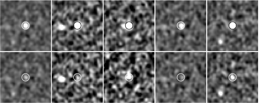
Figure 9.— Mean radio images of the KIERO subsamples in Table 1. The top row shows the results of $F_{1.4~{}\rm GHz}<600~{}\mu$Jy sources, and the bottom row shows the results of $F_{1.4~{}\rm GHz}<20~{}\mu$Jy sources. From left to right are all sources fainter than the above flux limits, $z<3$ sources, $z>3$ sources, ACS detected sources, and ACS undetected sources. Each panel has a size of $20\arcsec$. The small circles indicate our $3\arcsec$ flux apertures. The grayscale ranges in all panels are $-1.5$ to $3$ $\mu$Jy beam^-1.

In Figure 9 we show the stacked radio images of various KIERO subsamples. We start by discussing the top row, where we have applied a limit of $F_{1.4~{}\rm GHz}<600~{}\mu$Jy. The first thumbnail shows the stack of all the $F_{1.4~{}\rm GHz}<600~{}\mu$Jy sources. We then stacked the radio fluxes of the photometric redshift subsample of 76 KIEROs. These sources have, on average, higher 1.4 GHz fluxes than other KIEROs, since they are selected to be brighter in the NIR, and the radio flux correlates with the NIR flux. We find that the KIEROs at $z<3$ (second thumbnail) and the KIEROs at $z>3$ (third thumbnail) have similar mean radio fluxes. The observed radio flux for a given source has a redshift dependence of $F_{\rm radio}\propto(1+z)^{1-\alpha}/d_{L}(z)^{2}$, where $d_{L}$ is the luminosity distance. Using this relation and the measured mean radio fluxes, we find that KIEROs at $z>3$ are $\sim 2\times$ more radio luminous than KIEROs at $z<3$ (see also, Section 7 and Table 2). This may be because the 4.5 $\mu$m selection is only sensitive to more luminous systems at higher redshifts.

We also stacked the radio fluxes of the ACS-detected (fourth thumbnail) and the ACS-undetected (fifth thumbnail) KIEROs. There is a striking anti-correlation between the radio fluxes and the optical fluxes of KIEROs. The ACS-undetected subsample is, on average, $2.5\times$ brighter than the ACS-detected subsample in the radio. The same anti-correlation is also clearly observed when using 850 and 1100 $\mu$m fluxes rather than radio fluxes (see next section). This shows that the most active star forming galaxies in the universe are deeply hidden in dust and can hardly be traced with rest-frame UV observations, even with the extremely deep ACS observations in the GOODS-N.

It is also important to ask whether the above results are general properties of the entire KIERO population, or are biased by a few bright sources. In order to investigate this, we removed sources brighter than 20 $\mu$Jy in the radio (dotted line in Figure 8) and repeated the same stacking procedures. We adopted the same 20 $\mu$Jy cut in the Monte Carlo determinations of the confusion effect. The stacking results are listed in the lower half of Table 1. As expected, all the mean fluxes decrease, but they are still greater than at least 1.5$\sigma$. The general pattern is similar: the KIERO population is, on average, brighter in the radio than the 4.5 $\mu$m sources; and the ACS-undetected KIEROs are brighter in the radio than the ACS-detected KIEROs. We show some of the results in the bottom row of Figure 9, where we have applied the $F_{1.4~{}\rm GHz}<20~{}\mu$Jy limit. The thumbnail images correspond to all of the KIEROs below this limit (first), only the $z<3$ sources (second), only the $z>3$ sources (third), only the ACS-detected sources (fourth), and only the ACS-undetected sources (fifth).

In Figure 8 we see that nearly all (85 out of 86) sources with $F_{4.5~{}\rm\mu m}<1~{}\mu$Jy are below the 20 $\mu$Jy radio flux cut. Their stacked radio flux is $0.42\pm 0.76$ $\mu$Jy, or $0.18\pm 0.73$ $\mu$Jy after removing the one $>20~{}\mu$Jy source. Both are consistent with a null detection. On the other hand, if we look at sources with $F_{4.5~{}\rm\mu m}>1~{}\mu$Jy, the positive signal in their radio fluxes is very clear. In the $F_{4.5~{}\rm\mu m}=1$–3.2 $\mu$Jy bin, the mean radio flux is $6.76\pm 0.90$ $\mu$Jy for 65 sources, or $3.44\pm 0.88$ after excluding the six $>20~{}\mu$Jy sources.

We conclude that the majority of the NIR bright ($F_{4.5~{}\rm\mu m}>1~{}\mu$Jy) KIEROs are luminous in the radio, especially the optically faint sub class. This is true even if we remove radio detected KIEROs from the sample. On the other hand, the NIR faint ($F_{4.5~{}\rm\mu m}<1~{}\mu$Jy) KIEROs (43% of the total KIERO population) do not have detectable radio emission. In Section 7, we will use the stacked radio fluxes to study the star formation properties of KIEROs.

5.2. Millimeter and Submillimeter Properties

There exist numerous millimeter and submillimeter continuum surveys and follow-up studies in the GOODS-N (e.g., Hughes et al., 1998; Barger, Cowie, & Richards, 2000; Borys et al., 2003; Wang et al. 2004; Wang, Cowie, & Barger, 2006; Pope et al., 2006; Perera et al., 2008; Greve et al., 2008; Chapin et al., 2009). Here we considered two source catalogs, our SCUBA 850 $\mu$m catalog (Wang et al. 2004) and the AzTEC 1100 $\mu$m catalog (Perera et al., 2008), both with nearly complete multiwavelength identifications (Pope et al., 2006; Chapin et al., 2009). To be conservative, we only considered robust sources ($4\sigma$) with unambiguous 1.4 GHz identifications that we agree with, or with submillimeter interferometric identifications.

There are 28 850 $\mu$m and 1100 $\mu$m selected sources with such identifications in the IRAC area, 14 of which pass our $K_{S}-4.5$ $\mu$m $>1.6$ criterion. In addition, we found that several unidentified millimeter and submillimeter sources have nearby KIEROs within a few arcsec, sometimes multiple ones. The high fraction of submillimeter sources is consistent with our 1.4 GHz finding that we are selecting active star forming galaxies at high redshift with our KIERO selection.

We also stacked the millimeter and submillimeter fluxes of KIEROs. Here we used the 850 $\mu$m image of Wang et al. (2004) and the 1100 $\mu$m image of Perera et al. (2008). The stacking is similar to that in the radio. However, the caveat here is a possible upward bias caused by the coarse beams in the millimeter and submillimeter. If the stacked population has strong clustering at scales smaller or comparable to the beam, then the stacked flux would be positively biased. This was discussed by Wang et al. (2006) and Serjeant et al. (2008) and recently demonstrated by Marsden et al. (2009). Marsden et al. performed a stacking analysis using the deep Very Large Telescope (VLT) NIR sample of Grazian et al. (2006a, $5\times 10^{5}$ sources per deg²) in the GOODS-S and the BLAST 250–500 $\mu$m images (beam size $0\farcm 6$–$1\arcmin$). Their stacked far-IR (FIR) fluxes from the VLT NIR galaxies exceeded the FIR extragalactic background light (EBL) by factors of 2.5–3. The authors attributed this to small-scale clustering of the NIR selected galaxies, which shows a $\sim 100\%$ excess in the number of galaxies at scales of $\sim 1\arcmin$.

We performed a similar clustering analysis and found that our KIERO population only shows a 7% and 9% excess of sources within $15\arcsec$ (SCUBA beam FWHM) and $18\arcsec$ (AzTEC beam FWHM), respectively. This is much lower than the $\sim 100\%$ excess of the VLT NIR sample at the size scales of the BLAST beams. Thus, we conclude that stacking analyses of the GOODS-N SCUBA and AzTEC images using the KIERO population should not be biased by more than a few percent by small-scale clustering. (For comparison, we made similar tests on the entire $K_{S}$-band sample. There is a $\sim 30\%$ and $\sim 40\%$ excess of sources at size scales of $15\arcsec$ and $18\arcsec$, respectively.) After integrating the excess amounts convolved with the beam profiles, we found that these would bias the stacking results by up to 10%. This is likely an upper limit, since not all clustered objects are millimeter or submillimeter sources, as pointed out by Serjeant et al. (2008). We therefore conclude that bias caused by small-scale clustering in our sample is unlikely to affect our millimeter and submillimeter stacking results.

Instead of aperture photometry, the 850 and 1100 $\mu$m fluxes were measured with weighted point-source filters. The filtering and weighting schemes are described in Wang et al. (2004) and Perera et al. (2008). We measured the noise (sky, instrumental, and confusion noises) in the weighted fluxes and the flux bias (caused by random nearby sources) in a way identical to that for our radio stacking. Our noise measurements are 2.99 and 1.13 mJy per source for SCUBA and AzTEC, respectively. The flux biases are both zero, because of the zero sums of the beams. In our SCUBA image, there are two negative 50% sidelobes produced by the secondary chopping, producing a beam that has a zero total power. The PSF of AzTEC is more complex but the filtering function adopted by Perera et al. (2008) also has a zero sum.

Figure 10.— Millimeter and submillimeter fluxes vs. 4.5 $\mu$m flux for KIEROs. From the top we show stacked 1100 $\mu$m fluxes, 1100 $\mu$m fluxes of individual sources, stacked 850 $\mu$m fluxes, and 850 $\mu$m fluxes of individual sources. Individual sources enclosed in large squares are AGNs identified in Section 6. In the panels for stacked fluxes, solid squares show error-weighted stacked fluxes within bins of 1 dex in $F_{4.5~{}\rm\mu m}$ for the KIEROs. The exact values are shown near the symbols. Open squares show median fluxes for the same KIEROs in the same bins. For comparison, we show with downward triangles stacked fluxes from the 4.5 $\mu$m selected sample in 0.5 dex bins. Unlike the case in Figure 8, these are upper limits and may be overestimated by a few to $\sim 10$ percent because of small-scale clustering (see text). The 4.5 $\mu$m population is not detected at both 850 and 1100 $\mu$m at $F_{4.5~{}\rm\mu m}<1$ $\mu$Jy, despite the great numbers of sources there. The dotted lines correspond to roughly $5\sigma$. Stacking results for faint sources below these lines are presented in the lower half of Table 1.

In Figure 10 we present the measured millimeter and submillimeter fluxes of the individual sources in the second and fourth panels, respectively, and the stacked fluxes in the first and third panels, respectively. We summarize the stacking results in Table 1. As was the case in the radio, the millimeter and submillimeter fluxes seem to correlate with the 4.5 $\mu$m flux. Unfortunately, the S/N here does not allow us to meaningfully break down the sample to further study this property. When compared to the entire 4.5 $\mu$m sample (open downward triangles in Figure 10), the KIERO selection picks up brighter objects, on average, which is also similar to the case in the radio.

We stacked the millimeter and submillimeter fluxes in the photometric redshift subsample. At both 850 $\mu$m and 1100 $\mu$m, the mean fluxes from $z>3$ sources are higher than those from $z<3$ sources. It is well know that the observed flux in the millimeter and submillimeter is not a strong function of redshift at $z\sim 1$ to 10 for a fixed luminosity (Blain & Longair, 1993). The weighted-combined 850 and 1100 $\mu$m result indicates that KIEROs at $z>3$ are $1.5\pm 0.4$ times more luminous than KIEROs at $z<3$ are, on average. This is consistent with the result from the radio stacking.

As in the radio stacking analyses, here we also investigate the contribution from faint sources. We removed 1100 $\mu$m data above 3 mJy and 850 $\mu$m data above 6 mJy (dotted lines in Figure 10), and repeated all the stacking procedures. The results are listed in the lower half of Table 1. The general trend here is very similar to that in the radio, but with worse S/N.

We compared the millimeter and submillimeter and 1.4 GHz stacked fluxes and obtained rough redshift estimates. This “millimetric redshift” method was first published by Carilli & Yun (1999) and independently developed by Barger, Cowie, & Richards (2000). Here we adopted the formula derived by Barger, Cowie, & Richards (2000),

$$z=0.98(S_{850}/S_{1.4~{}\rm GHz})^{0.26}-1.$$ (1)

In deriving this equation, Barger et al. assumed a radio spectral index of $\alpha=0.8$ and a submillimeter dust emissivity of $\beta=1.0$, and they used Arp 220 for flux normalization. Using our mean 850 $\mu$m flux, our mean 1100 $\mu$m flux extrapolated to 850 $\mu$m assuming $\beta=1.0$, and our mean 1.4 GHz flux for $z<3.5$, we find an error-weighted millimetric redshift of $z\sim 2.4$. Using the stacked fluxes on undetected sources, we find a consistent redshift of 2.6. Despite the large uncertainty of this method, the results are remarkably close to what would be expected from the photometric redshift distribution in Figure 5(a), which is unlikely to be a coincidence. The agreement between these two entirely independent redshift estimates strongly suggests that our photometric redshift estimates and stacked fluxes are fairly reliable.

5.3. X-Ray Properties

Seven of the 196 KIEROs are in the 2 Ms Chandra catalog (Alexander et al., 2003). These include the two spectroscopic KIEROs at $z=1.790$ and 2.578. If we assume $z>2$ for the remaining five and an X-ray photon index of $\Gamma=1.8$ (e.g, Barger, Cowie, & Wang, 2007), then all seven have either rest-frame hard or soft X-ray luminosities exceeding $10^{42}$ erg s^-1 and hence are X-ray AGNs. One of the seven sources is the very bright 627 $\mu$Jy radio source (source 58 in Figure 7). This extremely large radio flux and its $F_{1100~{}\mu\rm m}$ upper limit (1 mJy) cannot be explained by any known starburst SED at $z>0.5$. Thus, its radio emission is almost certainly powered entirely by an AGN. This justifies the exclusion of this source in our radio stacking analysis, since our main goal is to measure SFRs.

Unlike the radio image, the 2 Ms Chandra observations do not probe into the starburst regime at $z>2$, making it difficult to address whether the remaining 189 KIEROs contain significant X-ray AGN activity. At $z=2$ and $z=3$, a $10^{42}$ erg s^-1 X-ray luminosity corresponds to X-ray fluxes of $4.7\times 10^{-17}$ and $1.7\times 10^{-17}$ erg s^-1 cm^-2, respectively, for $\Gamma=1.8$. The sensitivity of the 2 Ms observations do not reach such flux limits, especially in the hard X-ray band (e.g., see error bars in Figures 11 and 12). Thus, KIEROs undetected by Chandra may still host $>10^{42}$ erg s^-1 X-ray AGNs.

Figure 11.— Hard X-ray (2–8 keV) flux vs. 4.5 $\mu$m flux for KIEROs. The bottom panel shows the X-ray fluxes of individual sources. Sources enclosed in large squares are AGNs identified in Section 6. The top panel shows the stacked X-ray fluxes in each 0.5 dex 4.5 $\mu$m flux bin, only for sources below the dotted line, which roughly corresponds to $5\sigma$. Solid squares are the mean fluxes for KIEROs. The exact values are also shown near the symbols. Triangles show the mean fluxes of the entire 4.5 $\mu$m sample in the same flux ranges. In the two lower 4.5 $\mu$m flux bins, both the KIERO sample and the 4.5 $\mu$m selected sample are not detected.

Figure 12.— Same as Figure 11 but in the soft X-ray (0.5–2.0 keV). The middle panel is a blowup of the bottom one.

We carried out stacking analyses on the hard (2–8 keV) and soft (0.5–2.0 keV) unfiltered X-ray images of Alexander et al. (2003) to understand the average X-ray properties of KIEROs. We measured X-ray fluxes using aperture diameters approximately $2\times$ the PSF FWHM. Since the FWHM of the Chandra images vary with distance from the field center, we adjusted the size of the aperture accordingly. We measured the background locally after masking the detected objects. We compared our X-ray flux measurements with those given in the 2 Ms catalog and found excellent agreement. We estimated the errors (caused by confusion and shot noise) in the stacked fluxes with Monte Carlo simulations of random sources, as we did in the longer wavebands.

The stacked hard and soft X-ray fluxes for all the 196 KIEROs are $\langle F_{HX}\rangle=2.9\pm 0.9\times 10^{-17}$ and $\langle F_{SX}\rangle=8.1\pm 1.4\times 10^{-18}$ erg s^-1 cm^-2. The hard X-ray value is close to the flux for X-ray AGNs, and the soft X-ray value falls significantly below. Again, to understand if these stacked fluxes are dominated by small numbers of bright X-ray sources, we applied flux cutoffs that are approximately $5\sigma$ in both hard and soft bands, indicated by dotted lines in Figures 11 and 12. We imposed the same cutoff in the Monte Carlo simulations, which allows us to greatly reduce errors caused by bright X-ray sources that get close to our targets by chance. Furthermore, we stacked the X-ray fluxes of the KIEROs according to their 4.5 $\mu$m fluxes, as we did in the longer wavebands. The results are presented in the top panels of Figures 11 and 12.

In Figure 11, the stacked hard X-ray fluxes are consistent with AGNs at $F_{4.5~{}\rm\mu m}>3$ $\mu$Jy. This suggests a significant AGN contribution in the $F_{4.5~{}\rm\mu m}$ brightest members of KIEROs. On the other hand, KIEROs with $F_{4.5~{}\rm\mu m}<3$ $\mu$Jy show no detectable hard X-ray fluxes, and all the stacked soft X-ray fluxes in Figure 12 are below the flux required for X-ray AGNs. This suggest that the majority of KIEROs do not host X-ray AGNs. In the following sections, we will further identify AGNs in the radio and mid-IR (MIR) and exclude these AGNs in our analyses of star formation properties.

5.4. MIPS 24 $\mu$m Properties

The Spitzer GOODS Legacy Program DR1+ data release provided a 24 $\mu$m catalog obtained with the Spitzer Multiband Imaging Photometer (MIPS; Rieke et al., 2004). The catalog has a 24 $\mu$m flux limit of 80 $\mu$Jy and has 1041 sources in our IRAC region. Among the 1041 sources, 18 are KIEROs. The fraction of KIEROs in the DR1+ 24 $\mu$m sample is thus 1.7%, lower than the fraction in the radio (5.1% of the 1.4 GHz sample of Morrison et al., 2010, Section 5.1). However, the 80 $\mu$Jy flux limit used in the DR1+ catalog is shallower than the true depth of the image. To search for fainter MIPS detected KIEROs, we first made a deep source extraction in the MIPS image with SExtractor (Bertin, & Arnouts, 1996). We looked for matches between KIEROs and faint 24 $\mu$m sources within $2\arcsec$ radii (approximately 1/3 of the PSF FWHM). We then inspected all the matches by eye to remove unreliable matches caused by nearby bright sources and noise spikes. In particular, there are KIEROs residing in crowded regions with several blended MIPS sources. We removed such KIEROs unless their are clearly associated with local 24 $\mu$m peaks. The above procedure increases the number of MIPS detected KIEROs to 27. Simple aperture photometry indicates that this pushes the 24 $\mu$m detection limit to slightly less than 50 $\mu$Jy, corresponding to approximately 5 $\sigma$. After this, the fraction of 24 $\mu$m detections among the sample of 196 KIEROs is 14%, comparable to the fraction of radio detected KIEROs, which is 11%. This similarity suggests that radio and 24 $\mu$m observations are roughly equally effective in picking up KIEROs.

There is, however, an additional complication in the 24 $\mu$m case. At $z>1$, multiple broad PAH emission and silicate absorption features enter the MIPS 24 $\mu$m band, producing both positive and negative selection biases that are strong functions of redshift. These strongly affect the observed 24 $\mu$m fluxes of KIEROs, since they are all at $z>1$. Because of this, using 24 $\mu$m fluxes to quantify the star formation activity in KIEROs is highly uncertain (see, e.g., Murphy et al., 2009; Rodighiero et al., 2010) and strongly depends on the assumed SED models. On the other hand, the SEDs of galaxies in the radio are simple power laws with very similar spectral indices, and the radio–FIR correlation is fairly insensitive to dust temperature. We thus only relied on the radio data to study the SFRs of KIEROs.

We did not attempt to probe deeper at 24 $\mu$m with stacking analyses given the large uncertainties in interpreting the results. Instead, we stacked the radio, millimeter, and submillimeter fluxes of the MIPS detected and undetected KIEROs, to see whether the stacked fluxes are dominated by the few 24 $\mu$m detected sources and hence whether there are also passive objects in the KIERO selection. First, the 27 MIPS detected KIEROs have mean 1.4 GHz, 1100 $\mu$m, and 850 $\mu$m fluxes of $42.1\pm 1.7$ $\mu$Jy (after excluding the $>600$ $\mu$Jy bright radio source), $1.94\pm 0.22$ mJy, and $6.15\pm 0.68$ mJy, respectively. All these values are approximately $4\times$ higher than the mean fluxes of all KIEROs listed in Table 1. This is not surprising since we expect the 24 $\mu$m detections to be very luminous at high redshift. The remaining non-MIPS KIEROs have mean 1.4 GHz, 1100 $\mu$m, and 850 $\mu$m fluxes of $5.0\pm 0.7$ $\mu$Jy, $0.27\pm 0.09$ mJy, and $0.45\pm 0.31$ mJy, respectively. The results are still significant, except at 850 $\mu$m where the sample size is small (72). Furthermore, if we exclude the $F_{1.4~{}\rm GHz}>20~{}\mu$Jy sources from our radio stacking analyses, as we did in Section 5.1, then the mean radio flux of the remaining 157 non-MIPS sources is $2.3\pm 0.5$ $\mu$Jy. This is comparable to the result of $2.6\pm 0.5$ $\mu$Jy for all $F_{1.4~{}\rm GHz}<20~{}\mu$Jy sources. We conclude that even sources undetected at 24 $\mu$m have significant radio, millimeter, and submillimeter emission. We do not find evidence for a passive population based on the 24 $\mu$m to 1.4 GHz data.

6. AGN Fraction

In Section 5.3, we found seven KIEROs detected in the Chandra 2 Ms catalog (Alexander et al., 2003). All seven sources are X-ray AGNs with soft or hard X-ray luminosities greater than $10^{42}$ erg s^-1. To obtain a more complete identification of X-ray AGNs, we measured the X-ray fluxes of KIEROs as we did in the X-ray stacking analyses. We found four additional sources with $>3\sigma$ X-ray fluxes and with X-ray luminosities exceeding $10^{42}$ erg s^-1. Therefore, there are 11 X-ray AGNs in our KIERO sample.

In the MIR, our previous work (Barger, Cowie, & Wang, 2008; Wang et al., 2010) had shown that the IRAC AGN selection techniques of Lacy et al. (2004) and Stern et al. (2005) will either be incomplete or highly contaminated by normal galaxies in a deep sample like this. Here we adopt the MIR power-law selection technique (Donley et al., 2007). We require that the objects have to be detected in all four IRAC bands, and we performed power-law fitting to their IRAC SEDs. Among the 196 KIEROs, 54 are bright enough to be detected in all IRAC bands, and 13 have SEDs that can be well fitted ($\chi^{2}$ probability $>90\%$) by red power laws. All of them have red IRAC spectral slopes with $\alpha>0.7$, consistent with them being AGNs. One of the 13 is detected by Chandra and is also an X-ray AGN.

In the radio, we estimated the rest-frame 1.4 GHz power of radio detected KIEROs using their photometric redshifts and assuming a synchrotron spectral slope of $\alpha=0.8$. We found two KIEROs with unusually large 1.4 GHz radio powers of $>10^{25}$ W Hz^-1. Neither is a MIR power-law AGN. One source is #58 in Figure 7, an X-ray AGN discussed in Section 5.3. Its photometric redshift is very likely to be a catastrophic failure caused by its unusual SED, but this does not affect its AGN identification. The other source is #70 in Figure 7. Its photometric redshift fitting appears reasonable, and thus the estimated rest-frame radio power is reliable. Its large radio power ($2.1\times 10^{25}$ W Hz^-1) requires a SFR of $>10^{4}~{}M_{\sun}~{}{\rm yr}^{-1}$ (see next section), which is not supported by its infrared properties (e.g., it is undetected at 24 $\mu$m). We thus conclude that its radio emission is powered by an AGN.

The above X-ray, MIR, and radio selection identify 23 AGNs, which is 12% of the KIEROs in the GOODS-N. This fraction is a lower limit, since AGNs with lower X-ray, MIR, or radio luminosities would not be selected. On the other hand, all 23 AGNs are detected in the IRAC bands. Thus, the AGN fraction of the 54 members of the IRAC-bright subsample is $\sim 40\%$. This sets an upper limit on the AGN fraction of the entire KIERO sample since we expect to have more AGNs in luminous sources. Messias et al. (2010) studied AGNs in high-redshift extremely red galaxy populations using radio, X-ray, and MIR criteria. They found an AGN fraction of up to $\sim 30\%$, among which the majority are obscured MIR power-law AGNs. Their results are consistent with ours, given the small sample size here.

To see if the above AGN identification picks up X-ray AGNs that are below the Chandra detection limit, we repeat the hard X-ray stacking analyses in Figure 11 without all the above AGNs. In the 4.5 $\mu$m flux ranges of $>10$ $\mu$Jy and 3–10 $\mu$Jy, the stacked hard X-ray fluxes decrease substantially to $4.0\pm 2.5\times 10^{-17}$ and $0.3\pm 2.1\times 10^{-17}$ erg s^-1 cm^-2, respectively. Both values are not statistically significant. Therefore the above X-ray, MIR, and radio AGN identification is fairly effective in removing potential X-ray AGNs.

Table 2Star Formation Properties of KIEROs

Redshift	$N_{\rm galaxy}$	$\langle F_{1.4~{}\rm GHz}\rangle$	$\langle L_{IR}\rangle$	$\rm\langle SFR\rangle$	SFRD
		($\mu$Jy)	($10^{12}L_{\sun}$)	($M_{\sun}$ yr-1)	($M_{\sun}$ yr-1 Mpc-3)
All Sources
$z\sim 1.5$–2	10	$51.0\pm 2.7$	3.4	580	0.016
$z\sim 2$–3	27	$13.4\pm 1.7$	2.2	370	0.013
$z\sim 3$–4	23	$18.5\pm 1.8$	6.7	1150	0.036
$z\sim 4$–5.5	10	$31.3\pm 2.7$	20.8	3532	0.053
unknown	120	$2.5\pm 0.8$	$\cdots$	$\cdots$	$\cdots$
Non-AGNs
$z\sim 1.5$–2	9	$46.5\pm 2.9$	3.1	530	0.013
$z\sim 2$–3	22	$14.5\pm 1.9$	2.4	400	0.011
$z\sim 3$–4	15	$18.9\pm 2.2$	6.9	1170	0.024
$z\sim 4$–5.5	7	$7.3\pm 3.3$	4.8	820	0.009
unknown	115	$1.9\pm 0.8$	$\cdots$	$\cdots$	$\cdots$

7. Star Formation Rate

The SFRs of the KIEROs can be inferred from their total IR luminosities. Among all the flux measurements in Table 1, the radio fluxes provide the most robust estimates of the FIR luminosities. This is because the radio spectral slopes of normal galaxies are very similar and there is a tight correlation between radio and IR luminosity of normal galaxies, regardless of dust temperature (see the review of Condon, 1992). The latest FIR observations suggest that this correlation also holds for high-redshift galaxies (e.g., Ivison et al., 2010a, b; Bourne et al., 2011). An additional reason for using the radio is the higher S/N in the stacked radio fluxes.

A possible uncertainty of using radio fluxes for SFR estimates is the contribution from AGNs. In the previous section, we identified AGNs using X-ray, MIR, and radio data. This allows us to exclude AGNs from our sample. Furthermore, most of the KIEROs have radio fluxes well below 100 $\mu$Jy. At $z\sim 3$ this flux corresponds to a radio power of $6\times 10^{24}$ W Hz^-1. In the local universe, AGNs dominate the radio luminosity function at $P_{1.4~{}\rm GHz}>10^{24}$ W Hz^-1 (e.g., Mauch & Sadler, 2007). On the other hand, at $z>1$, starbursts start to dominate sources around $10^{24}$ W Hz^-1, and the luminosity function of AGNs falls substantially below that of starbursting galaxies at lower radio powers (e.g., Cowie et al., 2004). Thus, it is plausible that the contributions from AGNs to the radio fluxes of our KIERO sample are negligible. Below we will show this is indeed the case using AGNs identified in the previous section.

We now derive the conversion between radio flux and SFR. The radio power can be calculated from

$$P_{1.4~{}\rm GHz}=4\pi d_{L}^{2}(1+z)^{\alpha-1}F_{1.4~{}\rm GHz},$$ (2)

where $d_{L}$ is the luminosity distance and $\alpha$ is the radio spectral slope. Here we assume $\alpha=0.8$. To calibrate the conversion between radio power and SFR, we assume the radio–FIR correlation (Condon, 1992)

$$q\equiv\log\left(\frac{L_{\rm FIR}}{3.75\times 10^{12}\rm W}\right)-\log\left(\frac{P_{1.4~{}\rm GHz}}{\rm WHz^{-1}}\right)$$ (3)

and the canonical $q$ value of 2.3. Using the SED templates in Silva et al. (1998), we found that for a broad range of FIR SEDs the total IR luminosity conventionally defined between 8 and 1000 $\mu$m is approximately $2\times$ that of the 40–120 $\mu$m FIR luminosity. With this conversion factor and the standard conversion between total IR luminosity and SFR in Kennicutt (1998),

$${\rm SFR}~{}(M_{\sun}~{}{\rm yr}^{-1})=1.7\times 10^{-10}L_{\rm IR}(L_{\sun}),$$ (4)

we derived

$${\rm SFR}~{}(M_{\sun}~{}{\rm yr}^{-1})=7.83\times 10^{-8}(1+z)^{\alpha-1}\left(\frac{d_{L}}{Mpc}\right)^{2}\left(\frac{F_{1.4~{}\rm GHz}}{\mu\rm Jy}\right).$$ (5)

This agrees with the conversion in Yun, Reddy, & Condon (2001) to within 10% and is $\sim 20\%$ higher than that in Bell (2003).

In Table 2 we present the star formation properties of the KIEROs based on the stacked radio fluxes. The upper half of the table is for all KIEROs, and the lower half is for KIEROs without X-ray, MIR, and radio AGNs. It can be seen that excluding AGNs only slightly decreases the mean radio fluxes, except in the highest redshift bin, where the stacked radio fluxes are significantly biased by the two radio AGNs. This supports the argument that most of the KIEROs have radio emission powered by star formation. Below we will limit our discussion to the non-AGN results.

For the sources with redshifts, the SFRs and IR luminosities are similar to those of local ultraluminous IR galaxies (ULIRGs; Sanders & Mirabel, 1996) such as Arp 220. They are also close to the lower end of typical dusty galaxies found by millimeter and submillimeter single-dish surveys ($L_{\rm IR}\gtrsim 10^{13}L_{\sun}$). This is what we expected for the KIERO color selection. It is difficult to estimate the SFRs of the KIEROs without redshifts. If their redshift distribution is similar to that of KIEROs with redshifts, then they would be roughly an order of magnitude less luminous, or luminous IR galaxies (LIRGs). On the other hand, it is possible that these $K_{S}$ and IRAC faint sources are at higher redshifts. A mean radio flux of 1.9 $\mu$Jy from $z\sim 3$–4 would imply a SFR of $\sim 10^{3}M_{\sun}~{}{\rm yr}^{-1}$ and a ULIRG luminosity. We can thus safely conclude that most of the KIEROs are at least LIRGs at high redshifts, and many of them are starbursting ULIRGs.

We investigated whether there is a correlation between stellar mass and SFR. We did this only in the $z=2$–4 range because of the sample size. For $z=2$–3, we divided the non-AGN KIEROs into three groups according to their stellar masses: $<10^{10}M_{\sun}$ (7 sources), $10^{10}$–$10^{11}M_{\sun}$ (11 sources), and $>10^{11}M_{\sun}$ (7 sources). Their stacked radio fluxes are, respectively, $12.7\pm 3.3$, $5.6\pm 2.6$, and $23.3\pm 3.3$ $\mu$Jy. For $z=3$–4, we divided them into two groups: $<10^{11}M_{\sun}$ (6 sources), and $>10^{11}M_{\sun}$ (9 sources). Their stacked radio fluxes are, respectively, $19.2\pm 2.9$ and $18.4\pm 3.5$ $\mu$Jy. There is not a convincing trend here, except for fluctuations likely caused by the small sample sizes. Therefore, even the most massive KIEROs in our sample are still actively forming stars, and there is no evidence for a significant number of massive and passive galaxies in the KIERO population. This is quite different than other high-redshift red galaxies. We believe this is because our KIERO color selection avoids the 4000 Å Balmer break (a signature of old stars) and primarily picks up galaxies with continuous red spectral slopes (a signature of dust extinction).

We estimated the contributions of KIEROs to the cosmic star formation, i.e., their SFRD. Normally, one would like to apply the $1/V_{max}$ method (Schmidt, 1968) for calculating volume. Here, since most of our sources are not individually detected in the radio, applying such a method is effectively introducing additional weighting according to their $K_{S}$ or 4.5 $\mu$m properties in the radio stacking analyses. It is unclear to us whether this would bias the results. Therefore, we simply adopt total comoving volumes in the four redshift bins in Table 2 for our survey area (0.06 deg²). The derived SFRD for the sources with redshifts are listed in the table and shown in Figure 13 (solid squares). These values are lower limits for the following reasons: (1) they are not corrected for the substantial incompleteness in the $K_{S}$ and 4.5 $\mu$m bands; (2) they do not include star formation in the KIEROs identified as AGNs; and (3) they do not include contributions from the KIEROs without redshifts. If we assume that the redshift distribution of the KIEROs without redshifts is similar to that of the KIEROs with redshifts, then the SFRD values in Table 2 would increase by 20% in all four redshift bins. On the other hand, if we assume that the KIEROs without redshifts are, on average, from higher redshifts, then their contribution to the SFRD would be substantial. For example, if we assume that they are at $z>3$, then the SFRDs at $z>3$ would increase by 60% (open squares in Figure 13).

The SFRD values we found are comparable to those for bright SMGs at similar redshifts (Chapman et al., 2005), but we note that not all the bright SMGs are KIEROs. In Wang et al. (2006), we found a nearly flat SFRD of $\sim 0.06$–0.15 $M_{\sun}$ yr^-1 Mpc^-3 at $z=1$–4, from our radio and 850 $\mu$m stacking analyses of a large 1.6 and 3.6 $\mu$m selected NIR sample (dashed line in Figure 13, while the dotted line shows the same SFRD maximally corrected for incompleteness in the $z=1$–3 range). Naively speaking, the KIEROs should be a subsample of the larger NIR sample of Wang et al. (2006). However, the CLEAN-like procedure employed in W10 for this work provides many more 3.6 and 4.5 $\mu$m detected sources and better photometry. By comparing the list of KIEROs with our 3.6 $\mu$m catalog compiled in 2006, we found that 45% of the KIEROs in the SCUBA area were missed by Wang et al. (2006). The missed KIEROs have a broad range of 3.6 $\mu$m fluxes and the same IRAC image is used in both works, so this is not an effect of different detection limits. Because of this, comparing the SFRD here with that in Wang et al. (2006) is not straightforward.

Figure 13.— Comoving SFRD. Solid squares are SFRDs derived from our radio stacking analysis on KIEROs with redshift information. Open squares further include the contributions from KIEROs without redshifts, by assuming $z>3$ for these $K_{S}$ and IRAC faint KIEROs (see text for details). Open diamonds and triangles are extinction corrected rest-frame UV results from Bouwens et al. (2009) and Reddy & Steidel (2009), respectively, for LBGs integrated to 0.04 $L^{\star}$. The dashed line shows the mean SFRD in Wang et al. (2006) at $z=1$–4, derived using a radio stacking analysis on a large NIR selected sample. It is approximately flat. The dotted line shows the SFRD in Wang et al. (2006) at $z=1$–3 assuming the maximum possible completeness correction in the submillimeter.

We also compare our SFRDs with recent extinction corrected rest-frame UV determinations from LBGs (Bouwens et al., 2009, open diamonds in Figure 13; Reddy & Steidel, 2009, open triangles). At $z>3$, the SFRD of the KIEROs is similar in magnitude to the SFRD of the extinction corrected LBGs. At $z<3$, the KIERO SFRD contribution becomes only $\sim 10\%$ of that of LBGs. This might be explained by the fact that KIEROs do not include all SMGs and therefore they only account for part of the dusty star formation. However, even the radio/submillimeter SFRD determined by stacking on a large NIR sample by Wang et al. (2006; dashed line in Figure 13) is significantly lower than the SFRD of the extinction corrected LBGs.

The extinction corrected SFRD of LBGs seems to be unusually large at $z\gtrsim 2$, compared to submillimeter and KIERO SFRDs. In Table 1 we showed that optically faint KIEROs are brighter in the radio, millimeter, and submillimeter than KIEROs detected by ACS. In Section 8.3, we find that KIEROs have very little overlap with LBGs. One important finding in Wang et al. (2006) is that most of the submillimeter EBL arises from galaxies with intermediate rest-frame colors, i.e., galaxies not as blue as LBGs. The combination of these points suggests that a substantial amount of high-redshift star formation cannot be traced by rest-frame UV emission, and that the total SFRD should be the sum of the SFRD from LBGs and the SFRD from dusty sources. This would give a very large total SFRD at $z\gtrsim 2$, which raises the question of whether the large extinction corrected LBG SFRD is overestimated.

Carilli et al. (2008) stacked radio fluxes of $z\sim 3$ LBGs in the COSMOS field and found that the radio inferred mean SFR of these LBGs is only 1.8 times the extinction uncorrected mean UV SFR. They pointed out that this is much smaller than the factor of $\sim 5$ generally adopted for high-redshift LBGs. Furthermore, Ho et al. (2010) could not detect the radio signal from $z\sim 4$ LBGs with an extremely deep radio stacking analysis in the GOODS-N and S fields. Their inferred radio SFR of $z\sim 4$ LBGs is only consistent with the extinction corrected UV SFR in Bouwens et al. (2009) if a 2 $\sigma$ radio flux upper limit is adopted. This result also suggests a discrepancy between the radio SFR and the dust-corrected UV SFR. The reason for this discrepancy is unclear. In addition to the possibilities discussed in Carilli et al. (2008), another possibility is the correlation between FIR flux and UV spectral slope (Meurer, Heckman, & Calzetti, 1999) assumed in many high-redshift LBG studies. Recent observations show substantial scatter in this correlation (Cortese et a., 2006; Howell et al., 2010; Wijesinghe et al., 2011), and this may contribute to the uncertainty in the UV extinction correction. This issue will require further investigation, especially once direct measurements of the FIR luminosities of LBGs with sensitive instruments such as ALMA and Herschel become available.

8. KIERO and Other High-Redshift Populations

8.1. IRAC Selected EROs

Yan et al. (2004) used the ACS $z^{\prime}$ (F850LP) image and the IRAC 3.6 $\mu$m image in the HUDF and found 17 IRAC selected extremely red objects (IEROs) with $z^{\prime}-3.6~{}\mu\rm m>3.25$ (also see Yan, 2008). Among our 196 KIEROs, 123 have $z^{\prime}$ detections at $>3\sigma$, and only 27 of them are above the IERO color cut. If we adopt the $3\sigma$ limits for $z^{\prime}$ undetected KIEROs, then the number of IEROs increases to 68. Thus, $>1/3$ of KIEROs are also IEROs. Among the 17 IEROs in Yan et al., five satisfy the KIERO color cut, including one $K_{S}$ undetected IERO. Thus, approximately 1/3 of IEROs are KIEROs. The cumulative density of IEROs with $K_{S}<25$ is $\sim 1.4$ arcmin^-2, more than $2\times$ higher than that of KIEROs even after a $K_{S}$ based completeness correction. From these points of view, KIEROs and IEROs are two different populations with roughly 30% overlap.

On the other hand, the KIEROs are remarkably similar to IEROs in many other properties. First, the 17 IEROs in Yan et al. have redshifts between 1.6 and 3.6, 11 of them between 2 and 3. This is almost identical to the redshift distribution for KIEROs (Figure 5a). Secondly, the SEDs of IEROs mostly consist of strong NIR components from massive populations of old stars, plus secondary rest-frame UV components from ongoing star formation. This is also very similar to the SEDs of KIEROs (Figure 7 and Section 4), except that some KIEROs are too faint in the optical for the rest-frame UV components to be detected. The stellar masses derived from the SED fitting for IEROs and KIEROs are also similar, approximately $10^{9.5}$–$10^{11.5}M_{\sun}$. In Section 2, we showed that 14 out of the 28 identified SMGs in the GOODS-N are KIEROs. If we include $J$-band upper limits, then 22 out of the 28 SMGs are IEROs. This fraction is even higher than KIEROs.

Furthermore, Messias et al. (2010) performed radio stacking analyses on several red galaxy populations including IEROs. They found a mean radio flux of $8.2\pm 1.9$ from 96 IEROs at $z=2$–3 after excluding 3 sources detected at $>3\sigma$, where 1 $\sigma$ is $\sim 14$–17 $\mu$Jy in their observations. With a similar $\sim 50$ $\mu$Jy cut in our stacking of $z=2$–3 KIEROs, the stacked radio flux is $7.5\pm 1.4$ $\mu$Jy, quite comparable to IEROs at similar redshifts. The only difference here is that nearly 10% of KIEROs (2 out of 27) are above the 50 $\mu$Jy flux cut, but only 3% of IEROs in Messias et al. (2010) are above this cut, indicating that the KIERO population contains more ULIRGs. However, within the numerical uncertainties, these two percentages could be consistent.

Why two such similar populations do not overlap much in terms of color properties and number densities is an interesting question. In the color–color diagram in Figure 14 we see that the IERO selection and the KIERO selection overlap at high redshift on dusty sources. The difference is in the low-redshift end. In the lower-right part of the diagram, early-type galaxies (including those not forming stars) enter the IERO selection at $z>1.5$ or so. Such galaxies do not enter the KIERO selection at $z<3$. The upper-left part of the diagram is more interesting, i.e., galaxies that are KIEROs but not IEROs. Such galaxies have blue $z^{\prime}-3.6~{}\mu\rm m$ colors that are consistent with starbursting galaxies at $z>6$, simply based on the color tracks. These KIEROs are not $z>6$ galaxies. Instead, as described in Section 4.3, they have two distinct stellar populations. Their massive and reddened stellar populations make them redder than the KIERO criterion, and the unobscured parts of their ongoing starbursts make them bluer than the IERO criterion. In short, IEROs contain more early-type galaxies, and KIEROs contain more dusty sources with ongoing star formation. We believe this is a consequence of the fact that the KIERO selection avoids the Balmer break but targets the red spectral slopes caused by strong dust extinction.

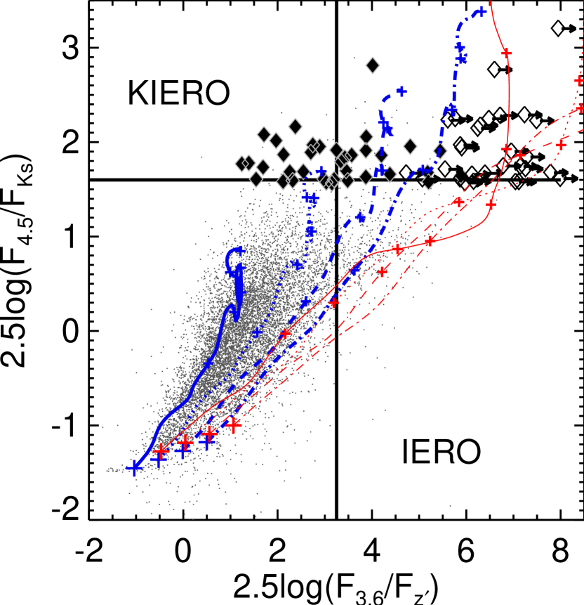
Figure 14.— $z^{\prime}$, $K_{S}$, and IRAC color–color diagram. The vertical and horizontal lines indicate the color criteria for IEROs and KIEROs, respectively. Color curves show the tracks of elliptical galaxies (thin red curves, Coleman et al. 1980) and starburst galaxies (thick blue curves, Kinney et al., 1996), reddened with the Calzetti et al. (2000) extinction law with $A_{V}=0$ (solid), 1.0 (dotted), 2.0 (dashed), and 3.0 (dash-dotted). Integer redshifts are indicated by crosses along the tracks, starting from $z=0$ in the lower-left and ending at $z=6$. Solid diamonds show KIEROs detected at both $K_{S}$ and $z^{\prime}$. Open diamonds with arrows show 1 $\sigma$ $z^{\prime}-3.6$ $\mu$m limits of $z^{\prime}$-undetected KIEROs. Dots in the background are field galaxies that are detected at $z$, $K_{S}$, and 3.6 $\mu$m at $>5$ $\sigma$.

8.2. Distant Red Galaxies

In addition to IEROs, distant red galaxies (DRGs, $J-K_{S}>1.35$; Franx et al., 2003) are another interesting population with which to compare. DRGs have redshifts roughly between 2 and 4 (e.g., van Dokkum et al., 2003; Föster Schreiber et al., 2004; Reddy et al., 2005), similar to KIEROs and IEROs. We therefore expect a substantial overlap between the DRG and KIERO populations. Unfortunately, there is not yet a $J$-band image in the GOODS-N that is sufficiently deep and wide to verify this. The CFHT WIRCam $J$-band image that we mentioned in Section 4 covers the entire GOODS-N with an rms depth of 0.09 $\mu$Jy (cf. 0.12 $\mu$Jy at $K_{S}$). Of the 104 $K_{S}$ detected KIEROs, only 37 are detected in this $J$-band image, and of those, only six have $J-K_{S}$ colors redder than 1.35. An additional 15 $J$ undetected KIEROs have $J$-band flux upper limits ($3\sigma$) satisfying the DRG color. Thus, at least 52 of the 104 $K_{S}$ detected KIEROs are DRGs, and the DRG fraction among the $K_{S}$ detected KIEROs can be anywhere between 50% and 70%.

There exists another $J$-band image around the HDF-N taken with the 8.2-m Subaru Telescope (Kajisawa et al., 2006). It is substantially deeper than the CFHT image. We carried out an independent reduction of this image (Wang et al., 2007), which covers $\sim 26$ arcmin² with an rms depth of $\sim 0.03$ $\mu$Jy. There are 16 $K_{S}$ detected KIEROs in this image. Five of them are detected in this deep $J$ image but all of them do not satisfy the DRG criterion. Five of the remaining six $J$-band undetected sources have $J$ upper limits that satisfy the DRG criterion. Thus, the fraction of $K_{S}$ detected KIEROs that are DRGs is anywhere between 30% and 70% based on this narrower and deeper $J$ image.

Finally, in the extremely deep HST NICMOS F110W image of the HDF-N (e.g., Dickinson et al., 2000; rms $\sim 0.15$ $\mu$Jy), there are only three KIEROs. Only one of them is detected in the $K_{S}$-band and it is not a DRG. However, this image is too narrow for us to draw a meaningful conclusion.

In terms of number density, the cumulative density of DRGs at $K_{S}<24$ is $\gtrsim 2$ arcmin^-2 (Labbé et al., 2003; Grazian et al., 2006b; Kajisawa et al., 2006), significantly higher than that for KIEROs (0.9 arcmin² at our $K_{S}$ and 4.5 $\mu$m limits). However, there is tentative evidence that the number density of DRGs starts to drop at $K_{S}>24$ (Kajisawa et al., 2006), while that of KIEROs still seems to be increasing at this magnitude (Section 3). If both observed trends are real, KIEROs are not just the faint-end tail of the DRGs. Based on the above results, we conclude that most DRGs are not KIEROs. On the other hand, a substantial fraction (perhaps $>50\%$) of KIEROs are DRGs, but not all. In Figure 15 we show the $J$, $K_{S}$, and 4.5 $\mu$m color–color diagram. It shows that the difference between DRGs and KIEROs is somewhat similar to that between IEROs and KIEROs.

Figure 15.— $J$, $K_{S}$, and 4.5 $\mu$m color–color diagram. The vertical and horizontal lines indicate the color criteria for DRGs and KIEROs, respectively. Curves are the same as those in Figure 14. Solid diamonds show KIEROs detected in both $K_{S}$ and $J$-band WIRCam images. Open diamonds with arrows show 1 $\sigma$ $J-K_{S}$ limits of $J$-undetected KIEROs. Dots in the background are field galaxies that are detected at $J$, $K_{S}$, and 4.5 $\mu$m at $>5$ $\sigma$.

In the SMG population, the fraction of DRGs is high. Among the 28 identified SMGs in the GOODS-N, 15 are DRGs. This fraction is comparable to the KIERO fraction in SMGs. Knudsen et al. (2005) studied the SFRs of DRGs in a lensing cluster field with a submillimeter stacking analysis at 850 $\mu$m. For DRGs with $K<24.4$ they found a mean 850 $\mu$m flux of 0.93 mJy and a mean SFR of 127 $M_{\sun}$ yr^-1 (both corrected for lensing amplification). Based on this, the typical SFRs of KIEROs are $\gtrsim 2\times$ higher than those of DRGs, despite being fainter in the NIR. On the radio side, Messias et al. (2010) performed radio stacking analyses on DRGs. They found a mean radio flux of $6.1\pm 1.6$ $\mu$Jy from 152 DRGs at $z=2$–3 after excluding 3 sources detected at $3\sigma$. As mentioned in Section 8.1, a similar stacking of $z=2$–3 KIEROs gives a comparable 7.5 $\mu$Jy radio flux, but the KIERO population has a higher ULIRG fraction.

8.3. Lyman Break Galaxies

To find LBGs in the 112 members of the ACS-detected subsample of KIEROs, we adopted the selection criteria of Beckwith et al. (2006) for galaxies in the HUDF. The selection criteria are also similar to those used by Bouwens et al. (2007). We found 15 $b$-dropouts, 4 $v$-dropouts, and 5 $i$-dropouts. This shows that most of the KIEROs are not LBGs, even for the subsample that is detected in the optical. The reason for this is that the spectral slopes are too red to be selected by the dropout criteria. Furthermore, the number of LBGs ($\sim 1700$ $b$-dropouts in GOODS-N; Bouwens et al., 2007) is much higher than the number of KIEROs (197 in GOODS-N). All these results imply that KIEROs and LBGs are two distinct populations.

It is important to realize that KIEROs are the most intensive starbursting galaxies at $z>2$, second only to the brightest SMGs. Their high SFRs (Section 7) imply strong rest-frame UV radiation. Without absorption, their redshifted optical fluxes would be roughly 1.6–2 $\mu$Jy at 0.5–1 $\mu$m. However, even in the ACS-detected KIERO subsample, most of them have optical fluxes lower than this (e.g., Fig. 7). The factor of almost 10 in the rest-frame UV dust attenuation in KIEROs is much larger than the generally accepted extinction corrections of $\sim 3\times$ to $5\times$ in LBGs (e.g., Bouwens et al., 2007; Reddy et al., 2008; Bouwens et al., 2009).

8.4. BzK Galaxies

The BzK selection (Daddi et al., 2004) is an effective technique for finding $1.4\lesssim z\lesssim 2.5$ galaxies. Since this redshift range overlaps with the lower-end of the redshift distribution of KIEROs, it is interesting to see where KIEROs fall on the BzK diagram (Figure 16). A difficulty here is that most KIEROs are optically faint, and we can only put a small subsample of KIEROs on the BzK diagram. Only 21 KIEROs are detected in all three of the $b$, $z^{\prime}$, and $K_{S}$ bands (squares), 14 of which are starburst BzK galaxies (sBzK). Sixteen KIEROs are detected in both the $z^{\prime}$ and $K_{S}$ bands (triangles), 11 of which have $b-z^{\prime}$ lower limits consistent with sBzK. The non-BzK KIEROs either have photometric redshifts that are too high or too low for the BzK selection (#15, 35, 53, and 55 in Figure 7) or have unusually blue rest-frame UV and optical SEDs (#44 and 63 in Figure 7) that barely miss the BzK selection.

We conclude that roughly 2/3 of the optically bright KIEROs are sBzK galaxies. However, the requirement of $b$ and $z^{\prime}$-band data makes the BzK selection less effective for extremely optically faint populations like the KIEROs. Finally, among the 28 identified SMGs, 13 are sBzK galaxies. This fraction is similar to the KIERO fraction in SMGs. However, as shown by Pannella et al. (2009) and Kurczynski et al. (2011), the BzK selection picks up much more “normal” star forming galaxies with SFR $\sim 10$–100 $M_{\sun}$/yr. The SMG fraction in BzK galaxies is much lower than the SMG fraction in KIEROs.

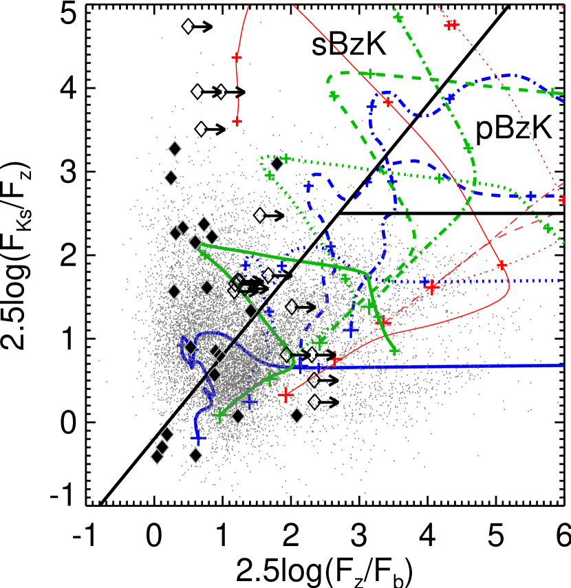
Figure 16.— $b$, $z^{\prime}$, and $K_{S}$ color–color diagram. The black diagonal and horizontal lines are the selection criteria for sBzK and pBzK galaxies. Curves are the same as those in Figure 14, except that we added Scd-type galaxies (green curves, Coleman et al. 1980). Solid diamonds are KIEROs detected at $K_{S}$, $z^{\prime}$, and $b$ bands. Open diamonds with arrows show 1 $\sigma$ $z^{\prime}-b$ limits of $b$-undetected KIEROs. Dots in the background are field galaxies that are detected in all three of the $b$, $z^{\prime}$, and $K_{S}$ bands at $>5$ $\sigma$. Squares are KIEROs that were detected in all three bands at $>3$ $\sigma$. Triangles show the lower limits for the KIEROs that are undetected in the $b$-band.

9. Discussion

9.1. Contributions to the Extragalactic Background Light

Our original goal of selecting extremely red sources from the $K_{S}$ and IRAC 4.6 $\mu$m bands was to see if we could select high-redshift dusty sources in the NIR. In this paper (Section 7) we showed that KIEROs are mostly LIRGs and ULIRGs at $z>2$. We found that KIEROs are optically faint. Their red optical SEDs imply that they will not be picked out as LBGs, even if they are detected in the optical. All of the results indicate that we have successfully selected a population of galaxies that are too dusty to be selected by existing optical and NIR surveys and too faint to be systematically detected with existing MIR, millimeter, and submillimeter surveys.

An interesting question is whether the KIERO sample includes the majority of ULIRGs at $z>2$. At 850 $\mu$m and 1100 $\mu$m, KIEROs have an integrated surface brightness of $4.47\pm 0.88$ and $1.64\pm 0.26$ Jy deg^-2 (Table 1), respectively. The EBL measured by the COBE satellite has strengths of 31–44 Jy deg^-2 at 850 $\mu$m and 18–25 Jy deg^-2 at 1100 $\mu$m. These were measured by two groups (Puget et al., 1996; Fixsen et al., 1998), and the range reflects the uncertainties in removing foreground contamination. Thus, KIEROs contribute approximately 10% to the EBL at these wavelengths and do not seem to represent the majority of sources that give rise to the millimeter and submillimeter EBL.

On the other hand, there is evidence that the majority of the millimeter and submillimeter EBL (especially at $\geq 850$ $\mu$m) arises at $z<2$ (Wang et al. 2006; Serjeant et al., 2008; Marsden et al., 2009), and thus that the KIERO selection may still pick up a large fraction of $z>2$ dusty sources. For example, Wang et al. (2006) found an 850 $\mu$m EBL contribution of $\sim 16$ Jy deg^-2 from a sample of 1.6 and 3.6 $\mu$m selected sources at $z<2$. This leaves at most 15–28 Jy deg^-2 to sources at $z>2$, of which $\sim 15\%$–27% can be attributed to the KIERO sample here. The actual fraction should be even larger considering the fact that the KIERO selection is still severely limited by completeness at $K_{S}$ and 4.5 $\mu$m. To determine whether or not KIEROs can fully account for the EBL that arises at $z>2$, we will need both a better determination of the KIERO number counts and a better EBL measurement.

9.2. Dust Hidden Star Formation

In Section 8.3 we showed that the dust attenuation of the rest-frame UV radiation of KIEROs is roughly a factor of 10 or even higher. It is now known that some of the most luminous millimeter or submillimeter selected galaxies can be entirely hidden by dust in the optical and even in the NIR (e.g., Wang, Barger, & Cowie, 2009; Cowie et al., 2009). The work presented here shows that there are still extremely extinguished galaxies when we go roughly an order of magnitude fainter in the total IR luminosity. Our KIERO color selection picks up such galaxies at $z\sim 1.5$–5, but the $K_{S}$ and IRAC images become less sensitive to galaxies at $z>3$. With a narrow selection window between $z\sim 2$ and 4 and the completeness limits in the $K_{S}$ and the 4.5 $\mu$m bands, we already pick up roughly 10% of the total EBL at 850 $\mu$m and 1100 $\mu$m. The total fraction of background that arises from extremely extinguished galaxies from $z=0$ to $>6$ should be even higher than this. We thus expect a significant fraction ($\gg 10\%$) of cosmic star formation to be entirely hidden from deep optical observations.

9.3. Nature of KIEROs

The KIERO color selection is meant to pick up objects with red spectral slopes over broad wavelength ranges and to avoid the 4000 Å Balmer break. This makes it sensitive to dusty starbursting galaxies. The fact that the KIEROs are selected near the peak of their stellar SEDs (i.e., the rest-frame 1.6 $\mu$m bump) also means that it is sensitive to massive systems. In Section 4 we showed that most KIEROs have stellar masses of $10^{10}$ to $10^{12}$ $M_{\sun}$. In Section 7 we showed that most KIEROs are ULIRGs with $L_{\rm IR}>10^{12}L_{\sun}$ and are actively forming stars. The masses of KIEROs are very similar to those of bright 850 $\mu$m selected SMGs at $z>2$ (e.g., Dye et al., 2008). On the other hand, the mean 850 $\mu$m flux of KIEROs (1.44 mJy) is below the confusion limit of single-disk telescopes. Its corresponding IR luminosity (assuming a dust SED similar to Arp 220) are a few times lower than those of most SMGs selected at 850 $\mu$m by single-dish telescopes. This suggests that KIEROs are massive galaxies undergoing slightly less intensive starbursts compared to bright SMGs.

In Section 2 we found that half of the identified SMGs in the GOODS-N are KIEROs. The fraction of SMGs that are DRGs is comparable (Sections 8.2), and the fraction of SMGs that are IEROs is significantly higher ($\sim 80\%$, Section 8.1). However, this does not mean that all of these color selections are equally efficient in picking up dusty sources. The IERO and DRG selections pick up substantial numbers of passive and $z<2$ galaxies (see also, Messias et al., 2010). However, in our radio stacking analyses of KIEROs, we did not see evidence for a significant subpopulation of passive KIEROs. This is true even after we introduce a 24 $\mu$m selection to our radio stacking analyses (Section 5.4). It is especially remarkable that approximately 1/3 of KIEROs are not detected by ACS. Such UV-faint sources would be considered as “passive” by many studies, but these KIEROs are even brighter in the radio than UV-bright KIEROs, indicating that they are more active in star formation. This distinguishes the KIERO selection from the IERO and DRG selections. We believe the KIERO selection is more effective in picking up dusty starburst galaxies and contains fewer passive galaxies.

In this paper we provide estimates of stellar masses and SFRs of KIEROs. Another crucial parameter for understanding the evolution is gas mass, which is not yet established for this new population of galaxies. Given the great similarity (SFRs, dust obscuration, and stellar masses) between KIEROs and bright SMGs, it is likely that the two populations are similarly massive in molecular gas mass. Recent observations of high-$J$ CO transitions of SMGs found molecular gas masses of a few $10^{10}M_{\sun}$ (Neri et al., 2003; Greve et al., 2005; Tacconi et al., 2006, 2008). If KIEROs are similarly rich in molecular gas, they can sustain their ultraluminous starburst phase for $\sim 100$ Myr. In other words, they can significantly increase their stellar masses in less than $10\%$ of their Hubble time.

To summarize, the KIERO selection seems to pick up a sample of massive and dusty $z>2$ galaxies. They are forming stars actively. This is consistent with massive galaxies at $z>2$ that are still rapidly building up their mass. The properties of KIEROs are similar to their more luminous counterparts (SMGs), as well as to high-redshift massive galaxies selected in the IRAC bands (e.g., IEROs and DRGs; see also Mancini et al., 2009). In each of these various selections we are likely seeing different regions of the luminosity function or different stages in the formation of the most massive galaxies at $z>2$. Eventually these galaxies will become quiescent and passively evolve into the “downsizing” era. However, at high redshifts, most of them seem to be still active. Because of the dust obscuration, common for the most intensive star-forming systems, a complete view of such massive and active galaxies requires observations at both long and short wavelengths.

10. Summary

In order to find high-redshift, faint, dusty sources that may give rise to a significant fraction of the submillimeter EBL, we selected 196 KIEROs with extremely red colors of $K_{S}-4.5$ $\mu$m$>1.6$ in the 0.06 deg² GOODS-N region. The selected KIEROs have a range of 4.5 $\mu$m fluxes, mostly between 1 and 10 $\mu$Jy. Of the 196 KIEROs, 104 KIEROs are detected in the $K_{S}$ band, and the slope of the $K_{S}$ number counts for these sources is steeper than that of $K_{S}$ selected galaxies at similar flux levels, likely because KIEROs are at redshifts higher than $K_{S}$ selected galaxies. The counts also still seem to be rising at the $K_{S}$ detection limit of $\sim 0.3$ $\mu$Jy. Roughly 2/3s of KIEROs are detected in the optical by HST ACS. However, only 1/5 of the ACS-detected KIEROs are LBGs. The remaining ACS detected KIEROs all have optical continua that are too red to pass the LBG selection.

We performed a photometric redshift analysis on a $K_{S}$-bright subsample of 76 KIEROs. We found a redshift distribution between $z\sim 1.5$–5, with roughly 70% at $z\sim 2$–4. This redshift distribution is quite similar to that of bright SMGs, but with a bias to high redshift. Our photometric redshift analysis also shows large stellar masses of $10^{10}$–$10^{12}M_{\sun}$. We found that a significant fraction of KIEROs have SEDs that cannot be well fitted by simple stellar populations. They have massive old stellar components that are luminous in the NIR and ongoing starbursts that are detected in the optical.

We found that roughly half of the identified millimeter and submillimeter sources in the GOODS-N are selected as KIEROs, but such sources only represent 7% of the selected KIEROs. To study the radio, millimeter, and submillimeter properties of the remaining KIEROs, we carried out stacking analyses. We found that, on average, KIEROs are brighter than normal 4.5 $\mu$m selected galaxies by factors of $\sim 2$ and $\sim 6$–10 in the radio and in the millimeter and submillimeter, respectively. We also found that KIEROs undetected by ACS are $\sim 3$–4 times brighter in all these wavebands than KIEROs detected by ACS. We repeated the stacking analyses on KIEROs undetected in the radio, millimeter, and submillimeter. These faint KIEROs still possess detectable stacking signal, showing that their properties are not dominated by small numbers of bright sources. We also did not find evidence of passive KIEROs based on the 24 $\mu$m to radio data.

We identified AGNs in the KIERO sample with large X-ray and radio luminosities, and with MIR SEDs that are featureless red power laws. We identified 19 such sources, of which 2/3 are obscured AGNs identified in the MIR. We also found an AGN fraction of up to 1/3.

Using the local radio–FIR correlation of normal galaxies and the stacked radio fluxes of non-AGN KIEROs, we found that they are LIRGs and ULIRGs. The results are consistent with the KIEROs being a population of $z>2$ ultraluminous dusty galaxies that are slightly fainter than SMGs in the millimeter and submillimeter and undetected by single-dish surveys. Their large IR luminosities imply high SFRs of $\sim 300$–1200 $M_{\sun}$ yr^-1, and therefore a population of massive $z>2$ galaxies in rapid formation. We showed that KIEROs contribute roughly 10% to the total EBL at 850 and 1100 $\mu$m and up to 30% of the EBL at these wavelengths which arises from galaxies at $z>2$. Given that KIEROs and LBGs have very little overlap and that optically faint KIEROs are brighter in the radio, millimeter and submillimeter, these results indicate that a significant fraction ($\gg 10\%$) of cosmic star formation is hidden by dust and cannot be traced by rest-frame UV emission.

References

- Alexander et al. (2003) Alexander, D. M. et al. 2003, AJ, 126, 539
- Barger et al. (1998) Barger, A. J., Cowie, L. L., Sanders, D. B., Fulton, E., Taniguchi, Y., Sato, Y., Kawara, K., & Okuda, H. 1998, Nature, 394, 248
- Barger, Cowie, & Richards (2000) Barger, A. J., Cowie, L. L., & Richards, E. A. 2000, AJ, 119, 2092
- Barger, Cowie, & Wang (2007) Barger, A. J., Cowie, L. L., & Wang, W.-H. 2007, ApJ, 654, 764
- Barger, Cowie, & Wang (2008) Barger, A. J., Cowie, L. L., & Wang, W.-H. 2008, ApJ, 689. 687
- Beckwith et al. (2006) Beckwith, S. V. W., et al. 2006, AJ, 132, 1729
- Bell (2003) Bell, E. F. 2003, ApJ, 586, 794
- Bertin, & Arnouts (1996) Bertin, E., & Arnouts, S. 1996, A&AS, 117, 393
- Blain & Longair (1993) Blain, A. W., & Longair, M. S. 1993, MNRAS, 264, 509
- Blain et al. (1999) Blain, A. W., Kneib, J.-P., Ivison, R. J., & Smail, I. 1999, ApJ, 512, L87
- Blanton & Roweis (2007) Blanton, M. R., & Roweis, S. 2007, AJ, 133, 734
- Bourne et al. (2011) Bourne, N., Dunne, L., Ivison, R. J., Maddox, S. J., Dickinson, M., & Frayer, D. T. 2011, MNRAS, 410, 1155
- Bolzonella, Miralles, & Pelló (2000) Bolzonella, M., Miralles, J.-M., & Pelló, R. 2000, A&A, 363, 476
- Borys et al. (2003) Borys, C., Chapman, S., Halpern, M., & Scott, D. 2003, MNRAS, 385, 398
- Bouwens et al. (2007) Bouwens, R. J., Illingworth, G. D., Franx, M., & Ford, H. 2007, ApJ, 670, 928
- Bouwens et al. (2009) Bouwens, R. J., et al. 2009, ApJ, 705, 936
- Brammer, van Dokkum, & Coppi (2008) Brammer, G. B., van Dokkum, P. G., & Coppi, P. 2008, ApJ, 686, 1503
- Bruzual & Charlot (2003) Bruzual, G., & Charlot, S. 2003, MNRAS, 344, 1000
- Calzetti et al. (2000) Calzetti, D., Armus, L., Bohlin, R. C., Kinney, A. L., Koornneef, J., & Storchi-Bergmann, T. 2000, ApJ, 533, 682
- Capak et al. (2004) Capak, P., et al. 2004, AJ, 127, 180
- Capak et al. (2008) Capak, P., et al. 2008, ApJ, 681, L53
- Carilli & Yun (1999) Carilli, C. L., & Yun, M. S. 1999, ApJ, 53, L13
- Carilli et al. (2008) Carilli, C. L., et al. 2008, ApJ, 689, 883
- Chapin et al. (2009) Chapin, E. L., et al. 2009, MNRAS, 398, 1793
- Chapman et al. (2000) Chapman, S. C., et al. 2000, MNRAS, 319, 318
- Chapman et al. (2003) Chapman, S. C., Blain, A. W., Ivison, R. J., & Smail, I. R. 2005, Nature, 422, 695
- Chapman et al. (2005) Chapman, S. C., Blain, A. W., Smail, I., & Ivison, R. J. 2005, ApJ, 622, 772
- Chen et al. (2011) Chen, C.-C., Cowie, L. L., Wang, W.-H., Barger, A. J., & Williams, J. P. 2011, ApJ, 733, 64
- Coleman, Wu, & Weedman (1980) Coleman, G. D., Wu, C.-C., & Weedman, D. W. 1980, ApJS, 43, 393
- Condon (1992) Condon, J. J. 1992, ARA&A, 30, 575
- Cortese et a. (2006) Cortese, L., et al. 2006, ApJ, 637, 242
- Cowie, Barger, & Kneib (2002) Cowie, L. L., Barger, A. J., & Kneib, J.-P. 2002, AJ, 123, 2197
- Cowie et al. (2004) Cowie, L. L., Barger, A. J., Fomalont, E. B., & Capak, P. 2004, ApJ, 603, L69
- Cowie et al. (2009) Cowie, L. L., Barger, A. J., Wang, W.-H., & Williams, J. P. 2009, ApJ, 697, L122
- Daddi et al. (2004) Daddi, E., Cimatti, A., Renzini, A., Fontana, A., Mignoli, M., Pozzetti, L., Tozzi, P., & Zamorani, G. 2004, ApJ, 617, 746
- Daddi et al. (2009a) Daddi, E., et al. 2009, ApJ, 694, 1517
- Daddi et al. (2009b) Daddi, E., Dannerbauer, H., Krips, M., Walter, F., Dickinson, M., Elbaz, D., & Morrison, G. E. 2009, ApJ, 695, L176
- Dickinson et al. (2000) Dickinson, M., et al. 2000, ApJ, 531, 634
- Donley et al. (2007) Donley, J. L., Rieke, G. H., Pérez-González, P. G., Rigby, J. R., Alonso-Herrero, A. 2007, ApJ, 660, 167
- Dye et al. (2008) Dye, S., et al. 2008, MNRAS, 386, 1107
- Fixsen et al. (1998) Fixsen, D. J., Dwek, E., Mather, J. C., Bennett, C. L., & Shafer, R. A. 1998, ApJ, 508, 123
- Föster Schreiber et al. (2004) Föster Schreiber, N. M., et al. 2004, ApJ, 616, 40
- Franx et al. (2003) Franx, M., et al. 2003, ApJ, 587, L79
- Giavalisco et al. (2004) Giavalisco, M. et al. 2004, ApJ, 600, L93
- Grazian et al. (2006a) Grazian, A., et al. 2006a, A&A, 449, 951
- Grazian et al. (2006b) Grazian, A., et al. 2006b, A&A, 453, 507
- Greve et al. (2005) Greve, T. R., et al. 2005, MNRAS, 359, 1165
- Greve et al. (2008) Greve, T. R., Pope, A., Scott, D., Ivison, R. J., Borys, C., Conselice, C. J., & Bertoldi, F. 2008, MNRAS, 389, 1489
- Ho et al. (2010) Ho, I.-T., Wang, W.-H., Morrison, G. E., & Miller, N. A. 2010, ApJ, in revision
- Howell et al. (2010) Howell, J. H., et al. 2010, ApJ, 715, 572
- Hughes et al. (1998) Hughes, D. H., et al. 1998, Nature, 394, 241
- Iono et al. (2006) Iono, D., et al. 2006, ApJ, 640, L1
- Ivison et al. (2010a) Ivison, R. J. 2010a, MNRAS, 402, 245
- Ivison et al. (2010b) Ivison, R. J. 2010b, A&A, 518, L31
- Kajisawa et al. (2006) Kajisawa, M., et al. 2006, PASJ, 58, 951
- Keenan et al. (2010) Keenan, R. C., Barger, A. J., Cowie, L. L., & Wang, W.-H. 2010, ApJ, 723, 40
- Kennicutt (1998) Kennicutt, R. C., 1998, ARA&A, 36, 189
- Kinney et al. (1996) Kinney, A. L., Calzetti, D., Bohlin, R. C., McQuade, K., Storchi-Bergmann, T., & Schmitt, H. R. 1996, ApJ, 467, 38
- Knudsen et al. (2005) Knudsen, K. K., et al. 2005, ApJ, 632, L9
- Knudsen, van der Werf, & Kneib (2008) Knudsen, K. K., van der Werf, P. P., & Kneib, J.-P. 2008, MNRAS, 384, 1611
- Kurczynski et al. (2011) Kurczynski, P., et al. 2011, submitted to ApJ (arXiv:1010.0290)
- Labbé et al. (2003) Labbé, I., et al. 2003, AJ, 125,1107
- Lacy et al. (2004) Lacy, M., et al. 2004, ApJS, 154, 166
- Maihara et al. (2001) Maihara, T., et al. 2001, PASJ, 53, 25
- Mancini et al. (2009) Mancini, C., Matute, I., Cimatti, A., Daddi, E., Dickinson, M., Rodighiero, G., Bolzonella, M., & Pozzetti, L. 2009, A&A, 500, 705
- Messias et al. (2010) Messias, H., Afonso, J., Hopkins, A., Mobasher, B., Dominici, T., & Alexander, M. 2010, ApJ, 719, 790
- Mauch & Sadler (2007) Mauch, T., & Sadler, E. M. 2007, MNRAS, 375, 931
- Marsden et al. (2009) Marsden, G., et al. 2009, ApJ, 707, 1729
- Meurer, Heckman, & Calzetti (1999) Meurer, G. R., Heckman, T. M., & Calzetti, D. 1999, ApJ, 521, 64
- Morrison et al. (2010) Morrison, G. E., Owen, F. N., Dickinson, M., Ivison, R. J., & Ibar, E. 2010, ApJS, 188, 178
- Murphy et al. (2009) Murphy, E. J., Chary, R. R., Alexander, D. M., Dickinson, M., Magnelli, B., Morisson, G., Pope, A., & Teplitz, H. I. 2009, ApJ, 698, 1380
- Neri et al. (2003) Neri, R., Genzel, R., Ivison, R. J., Bertoldi, F., Blain, A. W., Chapman, S. C., Cox, P., & Greve, T. R. 2003, ApJ, 597, L113
- Pannella et al. (2009) Pannella, M., et al. 2009, ApJ, 698, L116
- Peacock et al. (2000) Peacock, J. A., et al. 2000, MNRAS, 318, 535
- Perera et al. (2008) Perera, T. A., et al. 2008, MNRAS, 391, 1227
- Pope et al. (2006) Pope, A., et al. 2006, MNRAS, 370, 1185
- Puget et al. (1996) Puget, J.-L., Abergel, A., Bernard, J.-P., Boulanger, F., Burton, W. B., Désert, F.-X., & Hartmann, D. 1996, A&A, 308, L5
- Reddy et al. (2005) Reddy, N. A., Erb, D. K., Steidel, C. C., Shapley, A. E., Adelberger, K. L., & Pettini, M. 2005, ApJ, 633, 748
- Reddy et al. (2008) Reddy, N. A., Steidel, C. C., Pettini, M., Adelberger, K. L., Shapley, A. E., Erb, D. K., & Dickinson, M. 2008, ApJS, 175, 48
- Reddy & Steidel (2009) Reddy, N. A., & Steidel, C. C. 2009, ApJ, 692, 778
- Rieke et al. (2004) Rieke, G., et al. 2004, ApJS, 154, 25
- Rodighiero et al. (2010) Rodighiero, G., et al. 2010, A&A, 518, L25
- Sanders & Mirabel (1996) Sanders, D. B., & Mirabel, I. F. 1996, ARA&A, 34, 749
- Schmidt (1968) Schmidt, M. 1968, ApJ, 151, 393
- Serjeant et al. (2008) Serjeant, S., et al. 2008, MNRAS, 386, 907
- Silva et al. (1998) Silva, L., Granato, G. L., Bressan, A., & Danese, L. 1998, ApJ, 509, 103
- Smail, Ivison, & Blain (1997) Smail, I., Ivison, R. J., & Blain, A. W. 1997, ApJ, 490, L5
- Stern et al. (2005) Stern, D., et al. 2005, ApJ, 631, 163
- Tacconi et al. (2006) Tacconi, L. J., 2006, ApJ, 640, 228
- Tacconi et al. (2008) Tacconi, L. J., 2008, ApJ, 680, 246
- van Dokkum et al. (2003) van Dokkum, P. G., et al. 2003, ApJ, 587, L83
- Wang, Cowie, & Barger (2004) Wang, W.-H., Cowie, L. L., & Barger, A. J. 2004, ApJ, 613, 655
- Wang, Cowie, & Barger (2006) Wang, W.-H., Cowie, L. L., & Barger, A. J. 2006, ApJ, 647, 74
- Wang et al. (2007) Wang, W.-H., Cowie, L. L., van Sader, J., Barger, A. J., & Williams, J. P. 2007, ApJ, 670, L89
- Wang, Barger, & Cowie (2009) Wang, W.-H., Barger, A. J., & Cowie, L. L., 2009, ApJ, 690, 319
- Wang et al. (2010) Wang, W.-H., Cowie, L. L., Barger, A. J., Keenan, R. C., & Ting, H.-C. 2010, ApJS, 187, 251 (W10)
- Wang et al. (2011) Wang, W.-H., Cowie, L. L., Barger, A. J., & Williams, J. P. 2011, ApJ, 726, L18
- Webb et al. (2003) Webb, T. M., et al. 2003, ApJ, 582, 6
- Wijesinghe et al. (2011) Wijesinghe, D. B., et al. 2011, MNRAS, in press (arXiv:1103.3080)
- Yan et al. (2004) Yan, H., et al. 2004, ApJ, 616, 63
- Yan (2008) Yan, H. 2008, in AIP Conf. Proc. 996, Relativistic Astrophysics, e.d. C. L. Bianco, & S.-S. Xue, 71
- Yun, Reddy, & Condon (2001) Yun, M. S., Reddy, N. A., & Condon, J. J. 2001, ApJ, 554, 803
- Yun et al. (2008) Yun, M. S., et al. 2008, MNRAS, 389, 333