Molecular-dynamics simulation of clustering processes in sea-ice floes

Abstract

In seasonally ice-covered seas and along the margins of perennial ice pack, i.e. in regions with medium ice concentrations, the ice cover typically consists of separate floes interacting with each other by inelastic collisions. In this paper, hitherto unexplored analogies between this type of ice cover and two-dimensional granular gases are used to formulate a model of ice dynamics at the floe level. The model consists of: (i) momentum equations for floe motion between collisions, formulated in the form of a Stokes-flow problem, with floe-size dependent time constant and equilibrium velocity, and (ii) hard-disk collision model. The numerical algorithm developed is suitable for simulating particle-laden flow of $N$ disk-shaped floes with arbitrary size distribution. The model is applied to study clustering phenomena in sea ice with power-law floe-size distribution. In particular, the influence of the average ice concentration $\bar{A}$ on the formation and characteristics of clusters is analyzed in detail. The results show the existence of two regimes, at low and high ice concentration, differing in terms of the exponents of the cluster-size distribution and of the size of the largest cluster.

I Introduction

Recent global climate change, amplified in the polar regions of the earth, has led during the last decades to a substantial reduction of the ice extent, especially in the Arctic Serreze et al. (2007). This trend is strongly coupled to a decrease of the surface area covered with thick, multi-year ice, and a corresponding expansion of thin, seasonal ice-cover type Maslanik et al. (2007); Rothrock et al. (2008). Whether the thinning of the ice cover will eventually lead to permanently ice-free summers in the Arctic is still a subject of debate Serreze (2011). Undoubtedly, however, it substantially changes the response of the ice cover to the external forcing. Among other things, lower mechanical strength of thin ice makes it more susceptible to deformation, breaking and divergence. This kind of highly mobile ice cover, until recently occurring along the edges of the perennial ice pack (a so-called marginal ice zone, MIZ) and in subpolar, seasonally ice-covered seas, has been incomparably less intensively studied than the central Arctic ice pack. Global climate trends suggest that expanding our knowledge of the dynamics of this type of ice cover will become increasingly important in the future.

In this paper, a term ‘medium-concentration ice zone’ (MCIZ) is used rather broadly to describe a strongly fragmented ice cover type, consisting of clearly separated floes, with ice concentrations $\bar{A}<1$, i.e., in a dynamic regime between a free drift ($\bar{A}\ll 1$) and a compact ice cover ($\bar{A}\simeq 1$). Within MCIZ defined in this way, sea ice possesses a number of properties characteristic of granular materials – assemblies of discrete, macroscopic solid particles, interacting with each other via dissipative forces (e.g., friction and/or inelastic collisions). Dissipative nature of interactions is responsible for distinctive properties of granular materials, different from properties of fluids, solids and gases. For a review of collective properties and pattern formation in granular materials see, e.g., Aranson and Tsimring Aranson and Tsimring (2006).

Sea ice in MCIZ has all properties required to regard it as a particular subclass of granular materials: a two-dimensional (2D) granular gas. It consists of discrete solid floes (particles) immersed in water/air (‘interstitial fluids’) and moving on the sea surface due to the action of external forces of wind, currents etc. The floes can be regarded as rigid and indeformable. They collide inelastically, i.e., with a loss of kinetic energy. At medium ice concentrations floe–floe collisions contribute substantially to the internal stress in the ice Shen et al. (1984, 1986); Lu et al. (1989); Feltham (2005). Equations for the slowly-varying and random component of the floes’ velocity Feltham (2005) are fully analogous to those for dissipative gases Goldhirsch and Zanetti (1993); Brey and Cubero (2001). To the best of my knowledge, those analogies have never been explored in sea-ice modeling beyond the study by Feltham Feltham (2005) who applied granular flow theory to formulate a simplified MCIZ model with a composite collisional and plastic rheology, and showed that narrow zones of rapid ice movement along the MIZ edge (ice jets) can be obtained as an analytical solution to this model. It has been long recognized that collisional rheology is very different from the plastic one, routinely used in sea-ice models. However, the available collisional rheology models Shen et al. (1984, 1986); Lu et al. (1989), including the one used by Feltham, are based on unrealistic assumptions of floes of equal size or very narrow size distributions, uniformly distributed on the sea surface.

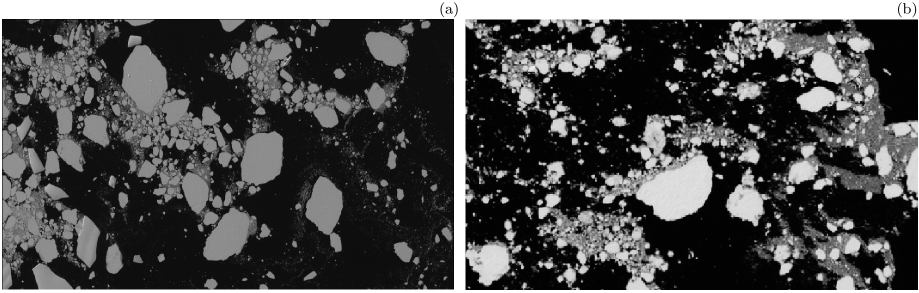
Figure 1: Fragments of Landsat images showing clustered sea-ice floes off the Antarctic coast (at 121.8^∘W, 73.5^∘S) on 18. Feb. 2008 (a) and 26. Jan. 2008 (b). Source: Lan (2011).

With all above-mentioned analogies between MCIZ and granular-gas dynamics in mind, there are a number of features that make sea ice unique among typically studied granular-gas problems. The most important of those features are, firstly, very wide, scale-free size distributions of ice floes, and secondly, size-dependent equilibrium velocities of floes under a given external forcing. The floe-size distributions (FSDs) observed in many ocean regions (see Inoue et al. (2004); Toyota et al. (2006); Steer et al. (2008); Herman (2010); Toyota et al. (2011) for recent works), are of power-law type $P(d)\sim d^{-1-\alpha_{r}}$, where $d$ denotes the floe diameter and $\alpha_{r}>1$. Most recent studies, based on combined satellite and airborne data covering a very wide range of floe sizes, showed the existence of two ‘regimes’ in FSDs for large and small floes, respectively, although the nature of the transition between those regimes has not been established yet Toyota et al. (2006); Steer et al. (2008); Herman (2010); Toyota et al. (2011). In this work, we assume for simplicity that $\alpha_{r}$ is a constant, and concentrate on the influence of the heavy FSD tail on the patterns of motion and cluster formation in MCIZ.

This study draws from the analogies between sea ice in MCIZ and granular gases, with a goal to develop a theoretical and numerical model of MCIZ dynamics at the floe level, and to explore the distinct behavior of sea ice compared to other, well studied granular-gas systems. Starting from well established equations of sea-ice motion, it is demonstrated that, under certain assumptions, the momentum equation describing the floe’s response to wind and current can be formulated as a Stokes-flow problem, with a floe-size dependent time constant and equilibrium velocity. Combined with a hard-disk (HD) model of floe–floe collisions, the Stokes equations are used to formulate a numerical model of MCIZ dynamics, in which, contrary to previous attempts, floe–floe interactions are simulated directly. In the further parts of this paper, the model is applied to study one of the fundamental aspects of granular-gas dynamics, namely formation of clusters due to irreversible loss of kinetic energy of colliding inelastic particles (see I.1 below). The general idea is that clusters of floes, observed in many real situations (Fig. 1; see also Toyota et al. (2011)), can be explained as an inherent property of sea ice, and not necessarily as a ‘passive’ result of the external forcing (convergence of surface currents).

A number of possible further applications of the model developed here are beyond the scope of this paper and will be explored elsewhere. They include formulation of internal-stress parametrization schemes suitable for MCIZ (at present, as mentioned above, only very crude collision-rheology models are available and in large-scale sea-ice models the internal stress is taken into account only at $\bar{A}\simeq 1$, see, e.g., Hunke and Lipscomb (2010)), and improved formulae for the atmosphere-ocean momentum and heat transfer in MCIZ. Some possible consequences of cluster formation in sea ice for the above processes, as well as the existence of possible feedbacks, are discussed at the end of this paper.

Apart from sea-ice modeling applications, the results of this work may be also of interest to researchers studying behavior of granular gases (particle-laden flows in particular) with wide particle-size distributions, which are still relatively unexplored theoretically and numerically Luding (2009). In particular, hitherto studies of clustering processes in polydisperse granular media concentrated either on binary or narrow size distributions Luding and Strauß (2001); Dahl et al. (2002); Rice and Hrenya (2010). The model and code developed here can be easily applied to other granular-gas systems consisting of particles with any given size distribution and size-dependent response to forcing.

The structure of this paper is as follows: further parts of the Introduction provide a brief theoretical background of cluster formation in granular gases, measures of cluster properties and methods of molecular-dynamics (MD) modeling of granular gases. Readers familiar with physics and modeling of granular materials may skip this part. In Section II, the equations of ice-floe motion are formulated in a way suitable for MD simulation. The model and its numerical implementation are described in Section III, followed by the presentation of the modeling results in Section IV. The paper concludes with a discussion in Section V.

I.1 Clustering in granular gases – mechanisms and cluster characteristics

In granular gases, clusters – regions with higher than average particle density – are initiated by random density fluctuations. Increased collision frequency in regions with higher density leads to a local decrease of the ‘granular temperature’ (kinetic energy associated with the random component of the particle motion, analogous to the thermodynamic temperature of gases), and thus to a local decrease in pressure. As a result, clusters tend to grow by attracting particles from their neighborhood, so that they may persist for a long time Goldhirsch and Zanetti (1993). This phenomenon is known from real dissipative granular systems and has been extensively studied numerically (e.g., Luding and Herrmann (1999); Dahl et al. (2002); Luding (2002); Miller and Luding (2004); Luding (2005); Rice and Hrenya (2009, 2010)). The tendency to form clusters, as well as their characteristic size, depend on the average properties of the system (particle density, coefficient of restitution, particle size and mass distribution, etc.), as well as on the external forcing. Most studies on granular materials consider equal-size and equal-mass particles. In the case of continuous size distributions, larger particles tend to accumulate in the central regions of clusters (a ‘self-sorting mechanism’, Rice and Hrenya (2010)).

A number of parameters can be defined for the purpose of a quantitative description of clustering processes. The most straightforward way of defining clustered/diluted regions is in terms of the local particle concentration $A$ relative to the average concentration $\bar{A}$ in the analyzed region (e.g., Rice and Hrenya (2009, 2010)). In this paper, another, distance-based approach is taken, i.e., the particles are assigned to clusters in such a way that every two particles separated by a distance smaller that $d_{m}$ belong to the same cluster (e.g., Miller and Luding (2004); Luding (2005)). Cluster properties are defined as averages and/or distributions of the properties of particles forming them, see Section IV. Additionally, a frequently used global measure of the spatial particle distribution is a radial distribution function $g_{rdf}(x)$, describing the expected particle concentration at a distance $x$ from the center of a randomly selected particle, normalized with $\bar{A}$ Luding and Strauß (2001); Rice and Hrenya (2009, 2010). This function is particularly suitable for monodisperse systems Luding and Strauß (2001), as it can provide a measure of characteristic cluster size. For polydisperse systems, floe–floe distance distribution $g_{ffd}(x)$ proposed in Section IV.2 seems more suitable.

I.2 Modeling of granular gases

At the core of an MD simulation is the detection of time and partners of collisions among a (usually very large) number of particles constituting the analyzed system. Hence, algorithms for solving typical fluid-dynamics problems, in which the time is advanced by prescribed, constant time steps, are unsuitable. Instead, event-driven algorithms (EDA) must be used Allen and Tildesley (1989); Sigurgeirsson et al. (2001). The choice of a proper EDA depends on (i) the character of motion of the particles between collisions, i.e., their interactions with the surrounding fluid, and (ii) the nature of particle–particle collisions. Most relevant for this work are algorithms designed for a subclass of dissipative-dynamics problems called particle-laden flows Sigurgeirsson et al. (2001), in which the motion of the fluid is given, i.e., it influences, but is not influenced by particles immersed in it.

Considering the material properties of sea ice it is justified to use a hard-disk (HD) collision model, assuming that at collision the momentum is transferred instantaneously along the line joining the centers of colliding particles (Allen and Tildesley, 1989). In other words, collisions are pairwise and infinitely short. EDAs for HD models are built based on event lists, in which times of collisions between all pairs of (potentially colliding) particles are stored and updated every time a collision takes place or particles’ velocities change. Available EDAs differ mainly in terms of how the event lists are updated, which may have a profound influence on the computational efficiency of those EDAs. For examples, see Marín (1997); Miller and Luding (2003) and a review by Sigurgeirsson et al. (2001).

II Assumptions and equations

Let us consider a set of $N$ disk-shaped, non-overlapping sea-ice floes with diameters $d_{i}$ ($i=1,\dots,N$), equal heights $h$ and constant density $\rho$, so that their mass centers coincide with their geometric centers. Due to the action of external forces, the floes move on the sea surface along trajectories $\mathbf{x}_{i}(t)$, where $\mathbf{x}_{i}\in\mathcal{A}$ denotes the position vector within an analyzed region $\mathcal{A}\subset\mathbb{R}^{2}$ and $t$ denotes time. The state of each floe at time $t$ is given by $(\mathbf{x}_{i}(t),\mathbf{u}_{i}(t))$, where $\mathbf{u}_{i}=\mathrm{d}\mathbf{x}_{i}/\mathrm{d}t$ denotes the floe’s translational velocity. Without interactions with neighboring floes, each floe moves independently and its acceleration can be determined from its state and the external forces, as described below. If the trajectories of floes intersect, they collide inelastically, with a loss of kinetic energy.

II.1 Floe motion between collisions

Between collisions, the motion of the $i$-th floe satisfies the momentum conservation equation (e.g., Leppäranta (2005)):

$$m_{i}\left({\mathrm{d}\mathbf{u}_{i}\over\mathrm{d}t}+f\mathbf{k}\times\mathbf{u}_{i}\right)=\int_{V_{i}}\mathbf{F}_{b,i}\mathrm{d}V+\int_{S_{i}}\mathbf{F}_{s,i}\mathrm{d}S,$$ (1)

where $\mathbf{k}=[0,0,1]$, $f$ denotes the Coriolis parameter, $m_{i}=\rho hS_{i}$ is the floe mass, $S_{i}=\pi d_{i}^{2}/4$ – its upper/lower surface area, and $\mathbf{F}_{b,i}$, $\mathbf{F}_{s,i}$ denote the sum of body and surface forces, respectively, acting on the analyzed floe. For simplicity, we will further assume that $f=0$ and $\mathbf{F}_{b,i}=0$ (in particular, the force resulting from the gradient of the geopotential height of the sea surface is not taken into account). The net surface force $\mathbf{F}_{s,i}$ results from a sum of four terms (Fig. 2): stress acting on the upper and lower surface of the floe (atmospheric and oceanic skin drag, $\boldsymbol{\tau}_{ha,i}$ and $\boldsymbol{\tau}_{hw,i}$, respectively), and pressure acting on the floe’s edges (atmospheric and oceanic body drag, $\boldsymbol{\tau}_{va,i}$ and $\boldsymbol{\tau}_{vw,i}$, respectively), see, e.g., Mai et al. (1996); Garbrecht et al. (2002); Lüpkes and Birnbaum (2005). The vertical surface area exposed to $\boldsymbol{\tau}_{va,i}$ and $\boldsymbol{\tau}_{vw,i}$ equals $d_{i}h_{f}$ and $d_{i}(h-h_{f})$, respectively, where $h_{f}=h(\rho_{w}-\rho)/\rho_{w}$ denotes the floe’s freeboard and $\rho_{w}$ denotes water density. (More realistically, the surface areas depend on the height/depth of ridges/keels, respectively, but this effect is not taken into account here.) Thus, (1) can be rewritten as:

$$m_{i}{\mathrm{d}\mathbf{u}_{i}\over\mathrm{d}t}=S_{i}(\boldsymbol{\tau}_{ha,i}+\boldsymbol{\tau}_{hw,i})+h_{f}d_{i}\boldsymbol{\tau}_{va,i}+(h-h_{f})d_{i}\boldsymbol{\tau}_{vw,i}.$$ (2)

In the following, the four forcing terms are parameterized with simple drag formulae typically used in sea-ice and ocean modeling. The atmospheric forcing depends quadratically on the wind speed $\mathbf{u}_{a}$:

$$\boldsymbol{\tau}_{ha,i}=\rho_{a}C_{ha}|\mathbf{u}_{a}|\mathbf{u}_{a},\quad\boldsymbol{\tau}_{va,i}=\rho_{a}C_{va}|\mathbf{u}_{a}|\mathbf{u}_{a},$$ (3)

where $\rho_{a}$ denotes the air density. The oceanic forcing depends on the floe velocity relative to the surface current $\mathbf{u}_{w}$. A quadratic relationship analogous to (3) is replaced with a linear one Leppäranta (2005):

$$\boldsymbol{\tau}_{hw,i}=\rho_{w}C_{hw}(\mathbf{u}_{w}-\mathbf{u}_{i}),\quad\boldsymbol{\tau}_{vw,i}=\rho_{w}C_{vw}(\mathbf{u}_{w}-\mathbf{u}_{i}).$$ (4)

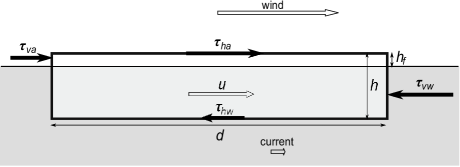
Figure 2: A side view of a disk-shaped ice floe under the action of wind and current. The arrows are not to scale. See the text for explanation of the symbols.

The drag coefficients $C_{ha}$, $C_{va}$, $C_{hw}$, and $C_{vw}$ are assumed constant. Linearization of $\boldsymbol{\tau}_{hw,i}$ and $\boldsymbol{\tau}_{vw,i}$ has important consequences for numerical algorithms used in the model, as it enables to formulate the governing equation (2) in the form mathematically analogous to the Stokes-flow problem Sigurgeirsson et al. (2001). Namely, from (2)–(4) we have:

$$\tau_{i}{\mathrm{d}\mathbf{u}_{i}\over\mathrm{d}t}=\mathbf{u}_{eq,i}-\mathbf{u}_{i},$$ (5)

where the time constant $\tau_{i}$ is given by:

$$\tau_{i}=\left[{\rho_{w}C_{hw}\over\rho h}+{4C_{vw}\over\pi d_{i}}\right]^{-1}.$$ (6)

After enough time and without interactions with other floes, each floe would reach its equilibrium ($\mathrm{d}\mathbf{u}_{i}/\mathrm{d}t=0$), free-drift velocity $\mathbf{u}_{eq,i}$, given by:

$$\mathbf{u}_{eq,i}=\mathbf{u}_{w}+C_{i}|\mathbf{u}_{a}|\mathbf{u}_{a},$$ (7)

where:

$$C_{i}=\tau_{i}\left[{\rho_{a}C_{ha}\over\rho h}+{4(\rho_{w}-\rho)\rho_{a}C_{va}\over\pi\rho_{w}\rho d_{i}}\right].$$ (8)

As can be seen, due to the form-drag effects $\tau_{i}$ and $\mathbf{u}_{eq,i}$ are floe-size dependent, as shown in Fig. 3 for a selected range of model parameters.

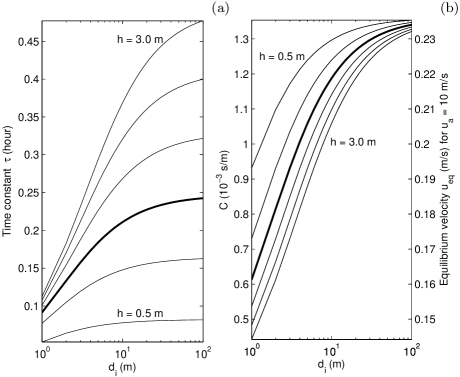
Figure 3: Time constant $\tau$ (a), coefficient $C$ and the equilibrium floe velocity $|\mathbf{u}_{eq}|$ for wind speed $|\mathbf{u}_{a}|=10$ m/s (b) in function of the floe diameter $d_{i}$, for a set of ice thickness values $h$. The lines are drawn every 0.5 m from $h=0.5$ m to $h=3.0$ m. Thick lines correspond to the model setup used in the simulations described in section IV (see Table 1).

II.2 Floe–floe collisions

Two floes, $i$ and $j$, moving along intersecting trajectories, collide at time $t_{c}$ which is the smallest positive root of the equation expressing the contact criterion for those floes:

$$||\mathbf{x}_{i}(t_{c})-\mathbf{x}_{j}(t_{c})||=(d_{i}+d_{j})/2.$$ (9)

As already mentioned, it is assumed that collisions are inelastic and infinitely short, and that they can be resolved via a HD model. If $\mathbf{u}_{i}$, $\mathbf{u}_{j}$ denote velocities just before collision, the post-collision velocities, $\tilde{\mathbf{u}}_{i}$ and $\tilde{\mathbf{u}}_{j}$, are given by:

$$\tilde{\mathbf{u}}_{i}=\mathbf{u}_{i}-m_{j}\mathbf{n}_{ij},\qquad\tilde{\mathbf{u}}_{j}=\mathbf{u}_{j}+m_{i}\mathbf{n}_{ij},$$ (10)

where:

$$\mathbf{n}_{ij}={1+\epsilon\over m_{i}+m_{j}}\left(\mathbf{k}_{ij}\cdot(\mathbf{u}_{i}-\mathbf{u}_{j})\right)\mathbf{k}_{ij},$$ (11)

and $\mathbf{k}_{ij}$ is a unit vector pointing from $\mathbf{x}_{i}$ to $\mathbf{x}_{j}$. The restitution coefficient $\epsilon\in[0,1]$ is assumed constant.

III The model

Like other MD models (see Section I.2), the one developed in this study – fancifully called the Small Floe Collider (SFC) – is based on an event-driven algorithm, suitable for particle-laden flows. SFC is capable of simulating a set of $N$ disc-shaped particles (‘floes’) with an arbitrary size distribution, within a square domain of side length $L$, with periodic boundaries. In order to simplify the treatment of periodic boundaries, during initialization the model domain is scaled to a region $[-1/2,1/2]\times[-1/2,1/2]$. All spatially-dependent variables ($d_{i}$, $|\mathbf{u}_{i}|$ etc.) are scaled accordingly. In order to speed up the simulations, the model domain is divided into $N_{c}$ square computational cells in order to reduce the search region for potential collision partners of a given floe. Consequently, two event types must be handled: floe–floe collisions (FFC) and virtual-wall collisions (VWC), corresponding to a transfer of a floe to a neighboring cell Sigurgeirsson et al. (2001).

Before we describe the SFC algorithm, two issues are worth discussing. Firstly, when discretizing the model equations, it should be noted that the floes’ trajectories between collisions can be determined exactly from equation (5). With initial conditions $\mathbf{u}_{i}(t_{0})=\mathbf{u}_{i,0}$ and $\mathbf{x}_{i}(t_{0})=\mathbf{x}_{i,0}$, we obtain easily, for $\Delta t=t-t_{0}$:

$$\mathbf{x}_{i}(t)=\mathbf{x}_{i,0}+\Delta t\mathbf{u}_{eq,i}-\tau_{i}(\mathbf{u}_{i,0}-\mathbf{u}_{eq,i})(e^{-\Delta t/\tau_{i}}-1).$$ (12)

Nevertheless, after inserting the floe positions given by (12) into the collision criterion (9), the resulting equation cannot be solved explicitly for $t_{c}$. Hence, (12) must be replaced with an approximate formula, allowing for a consistent calculation of floes’ positions and collision times. In SFC, the following linearly implicit integrator is used:

$$\mathbf{x}_{i}(t) = \mathbf{x}_{i,0}+\Delta t\mathbf{u}_{i,0},$$ (13)

$$\mathbf{u}_{i}(t) = \mathbf{u}_{i,0}+\Delta t/\tau_{i}(\mathbf{u}_{eq,i}-\mathbf{u}_{i}(t)).$$ (14)

It can be shown easily that using (13) amounts to replacing the exponential term in (12) with the first two terms in its series expansion ($e^{x}\approx 1+x$). From (12) and (13), the error of floes’ positions estimation can be calculated, and thus the maximum acceptable $\Delta t_{max}$ at which velocities must be updated. The error tends to be larger for smaller floes (because of both smaller $\tau_{i}$ and, typically, larger $|\mathbf{u}_{i}-\mathbf{u}_{eq,i}|$, see further section IV).

The second issue requiring some comment is related to the typical numerical problem of hard-sphere models: the inelastic collapse due to diverging collision rates between densely packed, almost touching particles. In SFC, it is accounted for by the method of Luding and McNamara Luding and McNamara (1998): if a given floe participates in more than one floe–floe collision within a certain time period $\Delta t_{c}$, corresponding to a collision duration, the restitution coefficient $\epsilon$ for those collisions is set to 1. In the simulations described in this paper, $\Delta t_{c}=10^{-1}$ s has been established experimentally as an optimal value.

The main part of the computational algorithm (Fig. 4) can be summarized as follows: At every iteration, the type of the nearest event, its partner(s) and time $t_{c}$ are determined. Subsequently, the model time $t$ is advanced by $\Delta t=t_{c}-t$, the floes are moved to their new positions, and the event is handled, accordingly to its type (FFC or VWC). In the final part of the main loop, the event lists are either updated only for the partners of the last event, or fully recalculated for all particles – depending on whether particle velocities have been updated at the current time step.

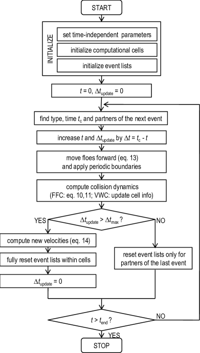
Figure 4: Flowchart of the SFC model.

IV Modeling results

In this section, the results of SFC simulations will be presented, with emphasis on the influence of the ice concentration $\bar{A}$ on cluster formation. A detailed analysis of model behavior in the full range of parameters ($|\mathbf{u}_{a}|$, $\epsilon$, $\alpha_{r}$ etc.) is beyond the scope of this study. The general results in terms of floes’ motion and cluster formation are described in Section IV.1. A more detailed analysis of the cluster properties and their size distribution is given in Sections IV.2 and  IV.3.

The model configuration is summarized in Table 1. In the simulations, the densities ($\rho$, $\rho_{w}$, $\rho_{a}$) and air-ice drag coefficients ($C_{ha}$, $C_{va}$) were set to their typical values found in literature (e.g., Leppäranta (2005)). The linear ice-water drag coefficients were estimated from their quadratic version ($\simeq 3.5\cdot 10^{-3}$) and equations (4,6–8) for $|\mathbf{u}_{i}|\simeq|\mathbf{u}_{eq,i}|$, assuming $C_{ha}=C_{va}$ and $C_{hw}=C_{vw}$. The surface current speed relative to the wind speed was estimated with the Ekman model Leppäranta (2005). For the ice floes properties, $h$, $\bar{d}$ and $\alpha_{r}$, typical values observed in the Weddell Sea during the ISPOL experiment Steer et al. (2008) were chosen. The mean ice concentration $\bar{A}$ was varied between the subsequent model runs in order to investigate its influence on the modeling results.

Table 1: Physical and numerical model parameters used in the SFC simulations

Parameter	Symbol	Value	Units
ice density	$\rho$	910	kg/m3
water density	$\rho_{w}$	1025	kg/m3
air density	$\rho_{a}$	1.23	kg/m3
air–ice skin-drag coef.	$C_{ha}$	$1.7\cdot 10^{-3}$	—
air–ice form-drag coef.	$C_{va}$	$1.7\cdot 10^{-3}$	—
water–ice skin-drag coef.	$C_{hw}$	$1.3\cdot 10^{-3}$	m/s
water–ice form-drag coef.	$C_{vw}$	$1.3\cdot 10^{-3}$	m/s
wind speed	$|\mathbf{u}_{a}|$	10	m/s
surface current speed	$|\mathbf{u}_{w}|$	$0.01|\mathbf{u}_{a}|$	m/s
ice thickness	$h$	1.5	m
mean ice concentration	$\bar{A}$	0.6–0.9	—
restitution coef.	$\epsilon$	0.85	—
FSD slope	$\alpha_{r}$	1.5	—
mean floe diameter	$\bar{d}$	2.0	m
No. floes	$N$	3000	—
No. computational cells	$N_{c}$	$10^{2}$	—
time step for vel. updates	$\Delta t_{max}$	1.0	s
collision duration	$\Delta t_{c}$	$10^{-1}$	s
No. ensemble model runs	$N_{ens}$	5	—

In all simulations, $\mathbf{u}_{a}=[u_{a},0]$ and the number of floes $N=3000$. (Larger system sizes were tested for $\bar{A}=0.6$ and $\bar{A}=0.8$, but no differences in terms of statistical properties of the results were recorded.) The floe radii $d_{i}$, $i=1,\dots,N$, were obtained with maximum-likelihood estimation for a power-law distribution with a given exponent $\alpha_{r}$ (see appendix A.1 for details). In each case, the size of the model domain was adjusted to the generated set of the floe diameters, to obtain the desired average ice concentration $\bar{A}$. For each set of model parameters, $N_{ens}=5$ ensemble model runs were performed, differing in respect of initial conditions, i.e., the floes’ initial velocities (drawn from a normal distribution with zero mean and standard deviation $1\cdot 10^{-2}$ m/s) and random positions. The optimal number of computational cells $N_{c}$, the time step for updating the floes’ velocity $\Delta t_{max}$, and the collision duration $\Delta t_{c}$ were established experimentally as $10^{2}$, 1.0 s and $0.1$ s, respectively. For $\Delta t_{max}$ and $\Delta t_{c}$, the largest values that had no significant influence on the modeling results were chosen.

In all cases, the model was run until a quasi-stationary state developed, characterized by insignificantly small temporal changes of such global variables as the total kinetic energy, collision rate and pressure. Comparisons between the ensemble model runs have shown that the initial conditions had no influence on the final values of those variables, although they may have influence on the details of the time evolution of the system towards the final state. The required number of iterations was established experimentally to $5\cdot 10^{6}$ FFC events.

IV.1 General properties of the solution

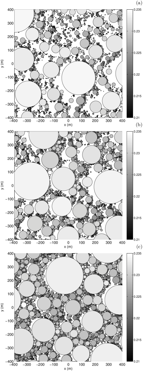
Figure 5: Snapshots (floe positions and velocities, in m/s, shown in gray scale) in a clustered state for $\bar{A}=0.6$ (a), $\bar{A}=0.725$ (b) and $\bar{A}=0.85$ (c). For better clarity, only equal-size fragments of the model domains are shown.

Figure 5 shows selected snapshots of the floes’ positions and velocities from three model runs with different $\bar{A}$. Contrary to the random initial state of the system, in the quasi-stationary regime the motion and distribution of the floes is patterned, with clearly developed clusters. Differently than in freely cooling granular gases, however, in the forced system under study the formation of clusters is strongly related to nonuniform equilibrium velocity of floes with different sizes. Larger floes tend to catch up with the smaller ones that accumulate in front of them and then slide along their sides, producing characteristic wakes. They are visible very well especially at small ice concentrations (Fig. 5a), but present even in densely packed ice-floe fields as narrow, elongated areas of open water upwind from large floes (Fig. 5c). Within clusters, the floes tend to stay in contact with each other. The translational velocity (i.e., velocity averaged over a certain number of collisions) is almost constant for all floes building a cluster. This translational motion is disturbed only if a cluster collides with another floe/group of floes. Unless such collision leads to a break-up of a cluster, velocities of floes constituting it remain highly correlated. As a result, the along-wind velocity of the largest floes within clusters is typically lower than their equilibrium velocity (Fig. 6a,c). This difference is larger for larger $\bar{A}$, i.e., higher collision rates. To the contrary, the smallest floes tend to move up to 30% faster than their equilibrium velocity, with a random component of velocity in the order of 1–3$\cdot 10^{-2}$ m/s, comparable to observed values, e.g. from the MIZEX experiment Shen et al. (1984, 1986). Understandably, the higher the ice concentration, the lower the differences between the largest and the smallest floes (Fig. 6c). Even though the differences $|\mathbf{u}_{i}-\mathbf{u}_{eq,i}|$ may be very large for individual floes, in all analyzed cases (i.e., independently of $\bar{A}$) the total momentum $\sum u_{i}m_{i}$ develops in time towards $\sum u_{eq,i}m_{i}$, which corresponds to floe-mass-weighted average velocity of $\sim$0.23 m/s. At high ice concentrations, this value roughly corresponds to the highest density of points in the along-wind velocity scatterplot (and to the velocity of the largest floes, Fig. 6c).

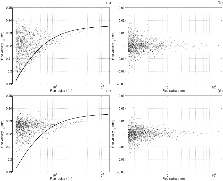
Figure 6: Scatterplots of instantaneous floe velocity components parallel (a,c) and perpendicular (b,d) to the wind direction, as a function of the floe radius $r$, for $\bar{A}=0.6$ (a,b) and $\bar{A}=0.9$ (c,d). The lines in (a) and (c) mark the equilibrium velocity $|\mathbf{u}_{eq}|$.

IV.2 Measures of clustering

Similarly as in observed clusters of ice floes (Fig. 1), the behavior of the system is dominated by the largest floes (Fig. 5). It is not surprising considering that among $N=3000$ power-law distributed floe diameters with $\alpha_{r}=1.5$, the largest floe occupies almost 10% of the total floe area $F_{tot}=\bar{A}L^{2}=\pi/4\sum_{i=1}^{N}d_{i}^{2}$, and the ten largest floes occupy over 46% of $F_{tot}$. This influence is clearly seen in the shape of the radial distribution functions of floes $g_{rdf}$ (see Section I.1). For the initial and final states of model runs with $\bar{A}=0.6$ and $\bar{A}=0.9$, $g_{rdf}$ is shown in Fig. 7. As can be seen, the dominating feature of $g_{rdf}$ is a pattern of shallow minima separated with narrow spikes corresponding to the radii of the largest floes, i.e., reflecting small floes densely packed along their edges. Interestingly, for $\bar{A}=0.9$, the number of small floes surrounding a very large one is roughly proportional to its perimeter; hence an approximately linear dependence of the height of the peaks of $g_{rdf}(x)$ on $x$ in Fig. 7c.

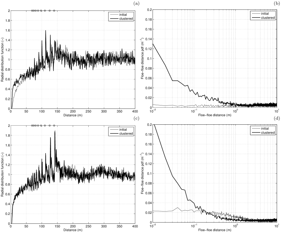
Figure 7: Radial distribution function $g_{rdf}$ (a,c) and floe–floe distance distribution $g_{ffd}$ (b,d) at the initial (random) and ‘final’ (clustered) phases for $\bar{A}=0.6$ (a,b) and $\bar{A}=0.9$ (c,d). Symbols along the upper border of (a) and (c) show radii of the eight largest floes in the sample.

The $g_{rdf}$ properties described above are present already in the initial, random floe distributions (in Fig. 7c the two curves are hardly distinguishable) and result simply from geometrical constraints of non-overlapping floes. Hence, $g_{rdf}$ is a poor indicator of the degree of clustering, especially for high ice concentrations (Fig. 7c). An alternative measure of clustering, suitable for very wide particle-size distributions, is therefore desirable. A straightforward candidate is a floe–floe distance distribution $g_{ffd}$, where the floe–floe distance is measured not between the floes’ centers, but between their edges ($x=||\mathbf{x}_{i}-\mathbf{x}_{j}||-r_{i}-r_{j}$ instead of $x=||\mathbf{x}_{i}-\mathbf{x}_{j}||$, as in $g_{rdf}$). For random floe distribution in space, $g_{ffd}$ is approximately distance-independent at small ice concentrations (Fig. 7b) and slightly increases toward zero in a densely packed ice field, again because of the above-mentioned geometrical constraints (Fig. 7d). However, in a clustered state $g_{ffd}$ increases rapidly (up to an order of magnitude) towards zero.

In the next section, the value of $d_{m}=0.5$ m was used to define clusters (see Section I.1). Other tested values from the range 0.1–1.0 m gave very similar results.

IV.3 Cluster size distribution

A deeper insight into cluster formation and properties can be gained from an analysis of cluster-size distribution. Let $N_{c}$ denote the number of clusters in the analyzed snapshot, and $\mathcal{C}_{k}$ – an $n_{k}$-element set of floes belonging to the $k$-th cluster ($k=1,\dots,N_{c}$ and $\sum_{k=1}^{N_{c}}n_{k}=N$). In the following, a total surface area of floes building the $k$-th cluster, $F_{c,k}$, is used as a measure of its size:

$$F_{c,k}={\pi\over 4}\sum_{i\in\mathcal{C}_{k}}d_{i}^{2}.$$ (15)

Because of generally very irregular shapes of clusters, especially at medium ice concentrations (Fig. 5), this quantity seems more appropriate than e.g. the area of the sea surface occupied by a cluster, which is difficult to estimate reliably (in particular, a straightforward convex-hull approach turned out inappropriate). Obviously, $\sum_{k=1}^{N_{c}}F_{c,k}=F_{tot}=\bar{A}L^{2}$. The effective cluster radius is given by $r_{e,k}=(F_{c,k}/\pi)^{1/2}$.

Figure 8 shows the rank-order distribution (see Appendix A.2) of $r_{e}$ in the final, quasi-stationary state for three values of $\bar{A}$: 0.6, 0.75 and 0.9. The distributions have two dominating features. Firstly, over most of the range of values they are of power-law type:

$$P(r_{e};\bar{A})\sim r_{e}^{-1-\alpha(\bar{A})}.$$ (16)

Secondly, the sizes of the largest clusters clearly deviate from the power-law regime, the more so the larger the ice concentration.

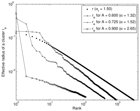
Figure 8: Rank-order distributions of effective cluster radius $r_{e}=(F_{c}/\pi)^{1/2}$ in fully clustered states for $\bar{A}$ equal 0.6, 0.725 and 0.9. Black dots show the corresponding distribution of the radii of single floes. Values are normalized so that $\pi\sum r_{e,i}^{2}=1$.

The exponents $\alpha$ of probability density functions $P(r_{e})$, estimated with a maximum likelihood method (equation 18 in Appendix A.2) increase with increasing $\bar{A}$, from values lower than $\alpha_{r}$ characteristic for low ice concentrations to values higher than $\alpha_{r}$ for densely packed ice fields (Fig. 9). The relationship between $\alpha_{r}$ and $\alpha$ suggests the existence of different mechanisms dominating cluster formation at low and high ice concentration. In the first case, typical clusters consist of the smallest floes accumulated along the downwind edges of the largest ones (Fig. 5a), because of large differences between the respective equilibrium velocities. This effect is also present during the initial stages of cluster development at higher ice concentrations (not shown), similarly leading to a transient decrease of $\alpha$. In other words, the smallest floes tend to belong to the largest clusters, without contributing much to $F_{c}$, dominated by the area of the largest floes. Hence, for the largest clusters their $r_{e}$s are hardly larger than the respective radii of their largest members.

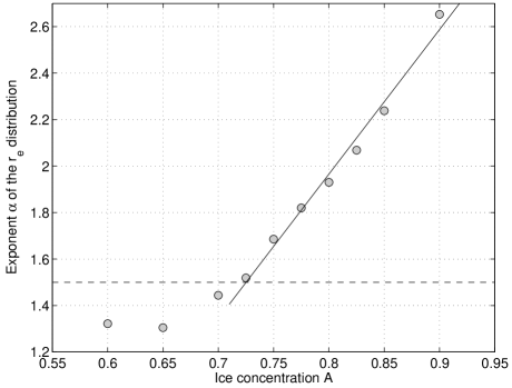
Figure 9: Exponent $\alpha$ of the distributions $P(r_{e})$ of effective cluster radii $r_{e}$ (equation 16) in function of the mean ice concentration $\bar{A}$. The horizontal dashed line shows the value of $\alpha_{r}=1.5$. The continuous line shows the linear least-square fit to the data for $\bar{A}>0.7$.

To the contrary, at high ice concentrations, due to high collision rates, the floes tend to move with similar translational velocity independently of their size (Fig. 6c). In this case, one large-scale cluster develops, spanning the whole model domain (Figs. 5c and 8). Only the smallest floes can gain enough kinetic energy at collisions so that they are able to escape the mega-cluster; and only the smallest floes find enough empty space in its ‘holes’ for an independent motion. This results in $\alpha>\alpha_{r}$. Finding a quantitative explanation for the observed dependence $\alpha(\bar{A})$, as shown in Fig. 9, is beyond the scope of this paper.

In terms of the dependence of the largest cluster size on the ice concentration, two regimes can be identified, as shown in Fig. 10. For $\bar{A}$¡$\sim$0.7, the area of the largest cluster remains comparable with the area of the largest floe in the sample (Fig. 8). For $\bar{A}\geq\sim 0.75$, one dominating mega-cluster develops, occupying over 85% of $F_{tot}$. Those two regimes are separated by a narrow range of medium, ‘critical’ ice concentrations $\bar{A}_{crit}$, characterized by a very interesting dynamics. Contrary to a relatively smooth development of the largest cluster in time, observed for both $\bar{A}\ll\bar{A}_{crit}$ and $\bar{A}\gg\bar{A}_{crit}$, the transitional range is associated with very strong, erratic temporal variations of the size of the largest cluster, corresponding to its constant rearrangement, break-ups and re-consolidation. In a sense, when judged by the size of the largest cluster, the system never reaches a quasi-stationary state for $\bar{A}\simeq\bar{A}_{crit}$.

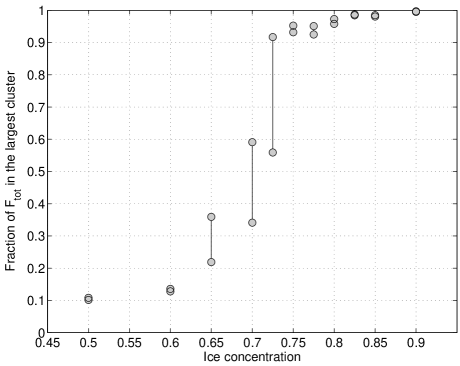
Figure 10: Surface area of the largest cluster $F_{c,1}$ (relative to the total surface area of all floes, $F_{tot}$) in function of the mean ice concentration $\bar{A}$. For each value of $\bar{A}$, the minimum and maximum values of $F_{c,1}$ recorded in the quasi-stationary state is shown.

Interestingly, in this transitional state the exponents $\alpha$ characterizing the cluster-size distribution $P(r_{e})$ are close to the value of $\alpha_{r}$ (Figs. 8 and 9), i.e., the cluster-size distribution $P(r_{e})$ mirrors $P(r)$. If $\alpha(\bar{A})$ is concerned, the critical range of $\bar{A}$ separates a region of slowly-varying values of $\alpha<\alpha_{r}$ from a region of fast, approximately linearly increasing values of $\alpha>\alpha_{r}$ (Fig. 9).

V Discussion and conclusions

The model presented in this paper describes a very idealized dynamics of MCIZ. Its purpose is rather to assist in understanding of basic processes regulating the formation of clusters in sea ice, than to reproduce details of any particular real-world situation. Qualitatively, the results of this study reproduce the dominant patterns of motion and clustering observed in MCIZ, including realistic granular temperature levels and clusters of small floes being pushed in front of a much larger one. Quantitative verification will require, on the one hand, experimental data on high-frequency sea-ice motion, unavailable at present, and on the other hand, more extensive simulations with a wide range of model parameters ($h$, $\mathbf{u}_{a}$, $\epsilon$, $\alpha_{r}$ etc.). Possible directions of future research include, but are not limited to: (i) formulation of an improved collisional rheology for MCIZ, based on internal-stress tensor components calculated with the SFC model, (ii) better understanding of the atmosphere–ice–ocean momentum transfer in MCIZ, resulting from the knowledge of the average motion of clustered ice fields in response to winds and currents, (iii) more detailed theoretical analysis of phenomena described in this paper, in particular explaining the dependence between the exponents of the floe-size and cluster-size distribution, and the nature of the transition between the two cluster-size regimes observed at low and high ice concentration, (iv) more detailed, in-depth analysis of the analogies between sea ice in MCIZ and other forced polydisperse granular media, and (v) analysis of the role of clustering in atmosphere–ocean heat transport and freezing/melting of the ice.

The last point is particularly interesting in view of a hypothesis formulated recently by Toyota and colleagues Toyota et al. (2011) who propose that cluster formation (or herding, in their nomenclature) may play a role in freezing of neighboring ice floes, and thus have an influence on the floe-size distribution in MCIZ. Combined with the results of the present study, this suggests an interesting possibility of a feedback between FSD and floe clustering. On the one hand, the FSD influences processes of cluster formation, including ice concentration within clusters and their size distribution. On the other hand, the existence of clusters may be important for floe formation in periods with low temperature, contributing to more intensive lateral freezing between densely packed floes. Clusters of floes frozen together are seen in satellite images of MCIZ (see Fig. 11 for an example of a Landsat image of the Okhotsk Sea). However, from a single snapshot it is not possible to determine the ‘life history’ of those floe formations. They could have been produced by freezing within already existing clusters, or – alternatively – they could have been a result of a divergence of an initially densely packed, frozen floe field and of subsequent random breaking of thin ice occupying spaces between thick floes. In the second case, the end result could have formed without the clustering–freezing–FSD feedback proposed above. Estimating the plausibility of that feedback is not possible without more observational data.

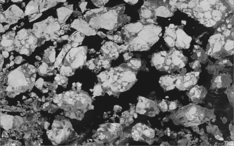
Figure 11: Fragment of a Landsat image of the Okhotsk Sea (3. Mar. 2003, 157.1^∘E, 58.7^∘N) with clusters of thick ice floes consolidated by thin ice. Source: Lan (2011).

Even though substantial progress has been made in recent years in observational techniques of the polar environment, including sea ice, MCIZ is still a very demanding, hard-to-explore medium. Consequently, even though it plays a crucial role in seasonal and long-term expansion and retreat of the ice cover in polar seas – one of important proxies of the climate change – the dynamics of MCIZ still remains poorly understood. Numerical models, like the one developed in this study, provide a valuable tool enabling to improve our knowledge and to gain more insight into functioning of that complex and fascinating environment.

Appendix A Rank-ordering statistics and maximum-likelihood estimation

To avoid drawbacks of binning in the analysis of distributions of the modeled quantities, rank-ordering technique is used throughout this paper Sornette (2006); Sornette et al. (1996). It is based on data sorted in descending order and – graphically – plotted versus the ranks (as in Fig. 8).

A.1 Calculation of the floe diameters

It is assumed that the floe-size probability density function (pdf) $P(d)$ is given by a power law $P(d)=Cd^{-1-\alpha_{r}}$ with $d>0$ and $\alpha_{r}>1$, so that the mean $\bar{d}$ exists. For prescribed $\alpha_{r}$, $\bar{d}$ and the finite sample size $N$, acting as a constraint, the maximum-likelihood estimation gives the most probable value of the $n$th of $N$ elements as (Sornette, 2006, p. 171):

$$d_{n}=\left[{\alpha_{r}N+1\over\alpha n+1}C\right]^{1/\alpha_{r}}.$$ (17)

The influence of the finite sample size is visible in the range of the largest elements in the sample: with decreasing $N$, the probability of encountering very large values decreases. This effect is seen in Fig.  8 as a deviation of the rank-order distribution of floe diameters from a straight line.

In the SFC model, formula (17) is used with $C=1$, and the obtained values are subsequently re-scaled so that $\sum_{n=1}^{N}d_{n}=N\bar{d}$. For a given ice concentration $\bar{A}$, the length $L$ of the computational domain is calculated as $L=(\pi/(4\bar{A})\sum_{n=1}^{N}d_{n}^{2})^{1/2}$.

A.2 Estimation of power-law exponents

Let $P(x)$ denote a power-law probability density function of variable $X$, represented by $N$ rank-ordered data points $x_{n}$ ($n=1,\dots,N$). A maximum-likelihood estimation $\alpha_{k}$ of the exponent $\alpha$ of $P(x)$, based on the sub-sample $(x_{k},x_{N})$, where ($1\leq k<N$), is given by Sornette (2006):

$$\alpha_{k}=N\left[\sum_{n=k}^{N}\log{x_{n}\over x_{N}}\right]^{-1}.$$ (18)

The standard deviation $\Delta\alpha_{k}$ of this estimate decreases with increasing sample size: $\Delta\alpha_{k}=\alpha_{k}(N-k+1)^{-1/2}$.

References

- Serreze et al. (2007) M. C. Serreze, M. M. Holland, and J. Stroeve, Science 315, 1533 (2007), doi:10.1126/science.1139426.
- Maslanik et al. (2007) J. A. Maslanik, C. Fowler, J. Stroeve, S. Drobot, J. Zwally, D. Yi, and W. Emery, Geophys. Res. Lett. 34, L24501 (2007), doi:10.1029/2007GL032043.
- Rothrock et al. (2008) D. A. Rothrock, D. B. Percival, and M. Wensnahan, J. Geophys. Res. 113, C05003 (2008), doi:10.1029/2007JC004252.
- Serreze (2011) M. C. Serreze, Nature 471, 47 (2011), doi:10.1038/471047a.
- Aranson and Tsimring (2006) I. S. Aranson and L. S. Tsimring, Rev. Modern Phys. 78, 641 (2006).
- Shen et al. (1984) H. Shen, W. Hibler III, and M. Leppäranta, MIZEX Bulletin III, USACREL Special Report 84-28 , 29 (1984).
- Shen et al. (1986) H. Shen, W. Hibler III, and M. Leppäranta, Acta Mechanica 63, 143 (1986).
- Lu et al. (1989) Q. Lu, J. Larsen, and P. Tryde, J. Geophys. Res. 94, 14525 (1989).
- Feltham (2005) D. Feltham, Phyl. Trans. Royal Soc. A 363, 1677 (2005), doi:10.1098/rsta.2005.1601.
- Goldhirsch and Zanetti (1993) I. Goldhirsch and G. Zanetti, Phys. Rev. Lett. 70, 1619 (1993).
- Brey and Cubero (2001) J. J. Brey and D. Cubero, in Granular Gases, Lecture Notes in Physics, Vol. 564, edited by T. Pöschel and S. Luding (Springer, Berlin–Heidelberg, 2001) pp. 59–78.
- Lan (2011) U.S. Geological Survey, http://glovis.usgs.gov/ (2011).
- Inoue et al. (2004) J. Inoue, M. Wakatsuchi, and Y. Fujiyoshi, Geophys. Res. Lett. 31, L20303 (2004), doi:10.1029/2004GL020809.
- Toyota et al. (2006) T. Toyota, S. Takatsuji, and M. Nakayama, Geophys. Res. Lett. 33, L02616 (2006), doi:10.1029/2005GL024556.
- Steer et al. (2008) A. Steer, A. Worby, and P. Heil, Deep-Sea Res. II 55, 933 (2008), doi:10.1016/j.dsr2.2007.12.016.
- Herman (2010) A. Herman, Phys. Rev. E 81, 066123 (2010).
- Toyota et al. (2011) T. Toyota, C. Haas, and T. Tamura, Deep Sea Res. II 9–10, 1182 (2011), doi:10.1016/j.dsr2.2010.10.034.
- Hunke and Lipscomb (2010) E. Hunke and W. Lipscomb, CICE: the Los Alamos Sea Ice Model Documentation and Software User s Manual Version 4.1, Tech. Rep. LA-CC-06-012 (Los Alamos National Laboratory, 2010) 76 pp.
- Luding (2009) S. Luding, Nonlinearity 22, R101 (2009).
- Luding and Strauß (2001) S. Luding and O. Strauß, in Granular Gases, Lecture Notes in Physics, Vol. 564, edited by T. Pöschel and S. Luding (Springer, Berlin–Heidelberg, 2001) pp. 389–409.
- Dahl et al. (2002) S. R. Dahl, R. Clelland, and C. M. Hrenya, Phys. Fluids 14, 1972 (2002).
- Rice and Hrenya (2010) R. B. Rice and C. M. Hrenya, Phys. Rev. E 81, 021302 (2010).
- Luding and Herrmann (1999) S. Luding and H. J. Herrmann, Chaos 9, 673 (1999).
- Luding (2002) S. Luding, C. R. Physique 3, 153 (2002).
- Miller and Luding (2004) S. Miller and S. Luding, Phys. Rev. E 69, 031305 (2004).
- Luding (2005) S. Luding, Pramana J. Physics 64, 893 (2005).
- Rice and Hrenya (2009) R. B. Rice and C. M. Hrenya, Phys. Rev. E 79, 021304 (2009).
- Allen and Tildesley (1989) M. P. Allen and D. J. Tildesley, Computer Simulation of Liquids (Oxford University Press, 1989) 408 pp.
- Sigurgeirsson et al. (2001) H. Sigurgeirsson, A. Stuart, and W.-L. Wan, J. Comput. Phys. 172, 766 (2001).
- Marín (1997) M. Marín, Computer Physics Communications 102, 81 (1997).
- Miller and Luding (2003) S. Miller and S. Luding, J. Comp. Phys. 193, 306 (2003).
- Leppäranta (2005) M. Leppäranta, The Drift of Sea Ice (Springer-Verlag, Berlin–Heidelberg–New York, 2005) 267 pp.
- Mai et al. (1996) S. Mai, C. Wamser, and C. Kottmeier, Bound. Layer Meteorol. 77, 233 (1996).
- Garbrecht et al. (2002) T. Garbrecht, C. Lüpkes, J. Hartmann, and M. Wolff, Tellus 54A, 205 (2002).
- Lüpkes and Birnbaum (2005) C. Lüpkes and G. Birnbaum, Bound. Layer Meteorol. 117, 179 (2005).
- Luding and McNamara (1998) S. Luding and S. McNamara, Granular Matter 1, 113 (1998).
- Sornette (2006) D. Sornette, Critical Phenomena in Natural Sciences, 2nd ed. (Springer Berlin–Heidelberg, 2006).
- Sornette et al. (1996) D. Sornette, L. Knopoff, Y. Y. Kagan, and C. Vanneste, J. Geophys. Res. 101B, 13883 (1996).