Inelastic electron transport through Quantum Dot coupled with an nano mechancial oscillator in the presence of strong applied magnetic field.

Abstract

In this study we explain the role of applied magnetic field in inelastic conduction properties of a Quantum Dot coupled with an oscillator . In the presence of strong applied magnetic field coulomb blockade effects become weak due to induced Zeeman splitting in spin degenerate eigen states of Quantum Dot.By contacting Quantum Dot by identical metallic leads tunneling rates of spin down and spin up electrons between Quantum Dot and electrodes will be symmetric. For symmetric tunneling rates of spin down and spin up electrons onto Quantum Dot, first oscillator get excited by spin down electrons and then spin up elctrons could excite it further. Where as average energy transferred to oscillator coupled with Quantum Dot by spin down electrons will further increase by average energy transferred by spin up electrons to oscillator. Here we have also discussed that with increasing Quantum Dot and electrodes coupling strength phononic side band peaks start hiding up, which happens because with increasing tunneling rates electronic states of  Quantum Dot start gettting broadened.

year number number identifier Date text]date

LABEL:FirstPage1 LABEL:LastPage#12

.1 Introduction

In recent years, much attention has been focused on the concept and realization of nanoelectromechanical systems (NEMS)1 ; 2 ; 3 ; 4 ; 5 ; 6 ; 7 ; 8 as a new generation of quantum electronic devices. A large number of new experimental techniques have been developed to fabricate and perform experiments with NEMS in the quantum regime. Examples of high-frequency mechanical nano-structures that have been produced are nano-scale resonators9 ; 10 , semiconductor quantum dots or single molecules11 ; 12 ; 13 ; 14 ; 15 ; 16 , cantilevers18 ; 19 , vibrating crystal beams9 , and more recently graphene sheets20 and carbon nanotubes21 ; 22 . These devices are expected to open up a number of future applications including nanomechanical transport effects, signal processing which could be used in fundamental research and perhaps even form the basis for new forms of mechanical computers. Many theoretical methods and models have been designed in order to account for the behavior of different types of NEMS system and to make predictions and proposals for future experiments.

In general, there are two different theoretical formulations that can be used to study the quantum transport in nanoscopic systems under applied bias. Firstly, a generalized quantum master equation approach23 ; 24 ; 25 ; 26 ; 27 ; 28 ; 29 ; 30 ; 31 ; 32 and secondly, the nonequilibrium Green’s function formulation33 ; 34 ; 35 . The former leads to a simple rate equation, where the coupling between the dot and the electrodes is considered as a weak perturbation and the electron- phonon interaction is also considered very weak. In the latter case one can consider weak and intermediate electordes to system and electron-phonon coupling. The nonequilibrium Green’s function technique is able to deal with a very broad variety of physical situations related to quantum transport at molecular levels36 ; 37 . It can deal with strong non-equilibrium situations and very small to very large applied bias. In the early seventies, the nonequilibrium Green’s function approach was applied to mesoscopic transport38 ; 39 ; 40 by Caroli et al., where they were mainly interested in inelastic transport effects in tunneling through oxide barriers. This approach was formulated in an elegant way41 ; 42 ; 43 by Mier et al, where they have shown an exact time dependent expression for the non-equilibrium current through mesoscopic systems. In this model an interacting and non-interacting mesoscopic system was placed between two large semi-infinite leads. In most of the theoretical work on NEMS devices since the original proposal, the mechanical degree of freedom has been described classically/semiclassically23 ; 44 or quantum mechanically24 ; 25 ; 26 ; 45 ; 46 using the quantum master or rate equation approach. In the original proposal, the mechanical part was also treated classically, including the damped oscillator, and assuming an incoherent electron tunneling process. This approach is based on a perturbation, weak coupling and large applied bias approximations, whereas the Keldysh nonequilibrium Green’s function formulation can treat the system leads and electron-phonon coupling with strong interactions47 for both small and large applied bias voltage. The transport properties have been described and discussed semi-classically/classically but need a complete quantum mechanical description. A theory beyond these cases is required in order to further refine experiments to investigate quantum transport properties of NEMS devices. In the quantum transport properties of these devices; the quantized current can be determined by the frequency of the quantum mechanical oscillator, the interplay between the time scales of the electronic and mechanical degrees of freedom, and the suppression of stochastic tunneling events due to matching of the Fermionic and oscillator properties.

In the present work, we consider a spin dependent electron transport through a quantum dot connected to two identical metallic leads via tunneling junctions. A single nanoelectromechanical oscillator is coupled with quantum dot and gate voltage is used to tune the levels on the dot. The application of strong magnetic field induce Zeeman splitting in spin degenrate eigen states of quantum dot. As a result spin down states moves lower and spin up states move higher than the degenrate spin eigen states of quantum quantum dot, and thus offers the different channels of conductance for spin up and spin down electrons. In the presence of strong applied magnetic field the coulomb blockade effects will be weak due to Zeeman splitting and we theoratically included it by mean field approximation, which is quite resonable approximation for tackling weak interactions. Although electron transport through mesoscopic systems in the presence of  Zeeman splitting has been an active area of research 57 ; 58 ; 59 . In our calculation the inclusion of the oscillator is not perturbative which enable us to predict strong electron phonons coupling effects in NEMS system. Hence, our work provides an exact analytical solution to the current-voltage characteristics, conductance, coupling of leads with the system, and it includes both the right and left Fermi- level response regimes. However, we have used wide-band approximation48 ; 49 ; 50 , where the coupling between leads and quantum dot is taken to be independent of energy. This provides a way to perform transient transport calculations from first principles while retaining the essential physics of the electronic structure of the quantum dot and the leads.

.2 Model Hamiltonian

Our mesoscopic system consists of a Quantum Dot(QD) coupled with an Oscillator to include the role of phonons effects in conduction through a QD. Application of external applied magnetic field induce Zeeman splitting in spin degenerate eigen states of QD. This constitute microscopic part of mesoscopic system.To incoporate coulomb blockade effects in QD we use mean field approximation which is useful for weak interaction. As in presence of strong magnetic field coulomb blockade effects will be small because of Zeeman splitting. Hamiltonian of the present microscopic system would be,

$$H_{QD+Oscillator}=\sum_{\sigma}(\epsilon_{\sigma}+\frac{1}{2}\mu_{B}g\sigma.B)d_{\sigma}^{{\dagger}}d_{\sigma}+\sum_{\sigma}\alpha_{\sigma}(a+a^{{\dagger}})d_{\sigma}^{{\dagger}}d_{\sigma}+\omega_{0}(a^{{\dagger}}a+\frac{1}{2})$$ (1)

The first term represents two discrete energy levels in QD, which orginates because of magnetic field induce Zeeman splitting. $d_{\sigma}^{{\dagger}},$ $d_{\sigma}$ $(a^{{\dagger}}a)$ create and annihilate an electron in state $|\sigma>$ on the dot (create and annihilate a phonon in state $|n>$ on the oscillator) . Here $\epsilon_{\sigma},$ $\mu_{B},g,\sigma,B,\alpha_{\sigma}$ and $\omega_{0}$ are energy levels of QD electronic-state with spin $\sigma$ ,Bohar magneton, Lande g factor,Pauli spin matrix, applied magnetic field, QD and oscillator coupling and oscillator vibrations frequency. Second term represents oscillator QD coupling and last term represents oscillator energy spectrum.

In first term of hamiltonian $\left(\sigma=1\right)$ for spin up electrons and $\left(\sigma=-1\right)$ for spin down electrons,

$$\epsilon_{\downarrow}=\epsilon_{o}\ ,\ \ \epsilon_{\uparrow}=\epsilon_{o}+U$$ (2)

where $U$ represents coulomb repulsion between spin down and spin up electrons.

To pass current through this sytem we employ left/right electrodes which constitues macroscopic part of of our system. Hamiltonian of left/right electrodes is

$$H_{Leads}=\sum_{k,\sigma}\epsilon_{k,\sigma,\nu}c_{k,\sigma,\nu}^{{\dagger}}c_{k,\sigma,\nu}.$$ (3)

Here $\epsilon_{k,\sigma,\nu}$ represents electrodes electronic states with wave vector $k$, spin $\sigma$ ,and electrodes $\upsilon$ (left/right). $c_{k,\sigma,\nu\text{ }}^{{\dagger}}(c_{k,\sigma,\nu})$ is electron creation (annhilation) operator in electrode $\upsilon$ .

Hopping of electrons between electrodes and QD is defined by the following Hamiltonian,

$$H_{Hopping}=\sum_{k,\sigma}(T_{k,\sigma,\nu}d_{\sigma}^{{\dagger}}c_{k,\sigma,\nu}+hermitian-congugation)$$ (4)

Here $T_{k,\sigma,\nu}$ represents electron hopping amplitudes between QD and electrodes.

We first solve our microscopic system Hamiltonian. Our approach include electron-phonon interaction exactly (non-perturbatively).

To diagonalize microscopic system Hamiltonain , we employ Lang-Firsov transformation51 .

$$\tilde{H}_{QD+Oscillator}=Exp[S]H_{QD+Oscillator}Exp[S^{{\dagger}}]$$ (5)

where

$$S=\sum_{\sigma}(a^{{\dagger}}-a)d_{\sigma}^{{\dagger}}d_{\sigma}$$ (6)

After diagonalization

$$\tilde{d}_{\sigma}^{{\dagger}}=d_{\sigma}^{{\dagger}}Exp[\frac{\alpha_{\sigma}}{\omega_{0}}(a^{{\dagger}}-a)$$ (7)

$$\tilde{d}_{\sigma}=d_{\sigma}Exp[-\frac{\alpha_{\sigma}}{\omega_{0}}(a^{{\dagger}}-a)$$ (8)

$$\tilde{a}^{{\dagger}}=a^{{\dagger}}-\frac{\alpha_{\sigma}}{\omega_{0}}d_{\sigma}^{{\dagger}}d_{\sigma}\text{ ,}\tilde{a}=a-\frac{\alpha_{\sigma}}{\omega_{0}}d_{\sigma}^{{\dagger}}d_{\sigma}$$ (9)

Therefore,

$$\tilde{H}_{QD+Oscillator}=\sum_{\sigma}(\epsilon_{\sigma}+\frac{1}{2}\mu_{B}g\sigma.B-\Delta_{\sigma})d_{\sigma}^{{\dagger}}d_{\sigma}+\omega_{0}(a^{{\dagger}}a+\frac{1}{2})$$ (10)

Where    $\Delta_{\sigma}=\frac{\alpha_{\sigma}^{2}}{\omega_{0}}$

Now the eigen function of the diagonalized Hamiltonian in k-space ( eigen function of harmonic oscillator remain same in real and Fourier’s space) would be

$$|o\sigma n>=\frac{1}{\sqrt{2}}\sum_{\sigma}A_{n}Exp[-\frac{k_{\sigma}^{2}}{2}]H_{n}[k_{\sigma}]Exp[-ik_{\sigma}x_{\sigma}]|\sigma>$$ (11)

$$|u\sigma n>=\frac{1}{\sqrt{2}}\sum_{\sigma}A_{n}Exp[-\frac{k_{\sigma}^{2}}{2}]H_{n}[k_{\sigma}]|\sigma>$$ (12)

$|o\sigma n>$ is state of occupied QD with electron and $|u\sigma n>$ is the state of un-occupied QD with electron.

Here $x_{\sigma}$ represents displacement of oscillator due to occupancy of electron in QD. $x_{\sigma}=\frac{\Delta_{\sigma}}{\omega_{0}}$ and $H_{n}[k_{\sigma}]$ are usual Hermite polynomials.

Now the amplitude of the occupied and un-occupied QD electronic state would be,

$$A_{mn\sigma}=<o\sigma m|u\sigma n>$$ (13)

$$A_{mn\sigma}=\frac{1}{\sqrt{\pi 2^{m+n+2}n!m!}}{\displaystyle\int}dk_{\sigma}Exp[-k_{\sigma}^{2}]H_{m}[k_{\sigma}]H_{n}[k_{\sigma}]Exp[ik_{\sigma}x_{\sigma}]$$ (14)

$$A_{mn\sigma}=\sqrt{\frac{2^{n-m-2}m!}{n!}}Exp[-\frac{x_{\sigma}^{2}}{4}][\frac{ix_{\sigma}}{2}]^{\left|n-m\right|}L_{m}^{\left|n-m\right|}[\frac{x_{\sigma}^{2}}{2}]$$ (15)

Here $L_{m}^{\left|n-m\right|}[\frac{x_{\sigma}^{2}}{2}]$ represents associated Lagurre’s polynomials.

After diagonalization tunneling Hamiltonian $H_{Hopping}$ will become,

$$\hat{H}_{Hopping}=\sum_{k,\sigma}(\hat{T}_{k,\sigma,\nu}d_{\sigma}^{{\dagger}}c_{k,\sigma,\nu}+hermitian-congugation)$$ (16)

Where$\left(\hat{T}_{k,\sigma,\nu}=T_{k,\sigma,\nu}Exp[\frac{\alpha_{\sigma}}{\omega_{0}}(a^{{\dagger}}-a)]\right)$

.3 Current from the mesoscopic system

Current from the $\left(\nu\right)$ electrode to the QD can be calculated by taking time derivative of occupation number operator of $\left(\nu\right)$ electrode.

$$J^{\nu}(t)=-e\left\langle\frac{\partial}{\partial t}N^{\nu}\right\rangle=ie\left\langle\left[N^{\nu},H\right]\right\rangle$$ (17)

where $\left(N^{\nu}=\sum_{k,\sigma}c_{k,\sigma,\nu}^{{\dagger}}c_{k,\sigma,\nu}\right)$ and $\left(H=\tilde{H}_{QD+Oscillator}+H_{Leads}+\hat{H}_{Hopping}\right)$ .Therefore,

$$J^{\nu}(t)=ie\sum_{k,\sigma}\left(\hat{T}_{k,\sigma,\nu}\left\langle c_{k,\sigma,\nu}^{{\dagger}}\tilde{d}_{\sigma}\right\rangle-\hat{T}_{k,\sigma,\nu}^{{\dagger}}\left\langle\tilde{d}_{\sigma}^{{\dagger}}c_{k,\sigma,\nu}\right\rangle\right)$$ (18)

$$J^{\nu}(t)=i2e\operatorname{Im}[\sum_{k,\sigma}\hat{T}_{k,\sigma,\nu}\left\langle c_{k,\sigma,\nu}^{{\dagger}}\tilde{d}_{\sigma}\right\rangle]$$ (19)

Now we define electrode and QD coupled lesser Green’s function,

$$G_{un\sigma,k\sigma}^{<}(t,t)=i\left\langle c_{k,\sigma,\nu}^{{\dagger}}d_{\sigma}\right\rangle$$ (20)

$$J^{\nu}(t)=i2e\operatorname{Im}[\sum_{k,\sigma}\hat{T}_{k,\sigma,\nu}G_{un\sigma,k\sigma}^{<}(t,t)]$$ (21)

To find electrode and QD coupled lesser Green’s function we utilize equation of motion technique (see43 ; 53 ; 54 ; 55 for utilizing equation of motion technique in non-equilibrium Green’s function theory),

$$\left(-i\frac{\partial}{\partial t^{\prime}}-\epsilon_{k,\sigma,\nu}\right)G_{un\sigma,k\sigma}^{t}(t-t^{\prime})=\hat{T}_{k,\sigma,\nu}^{{\dagger}}G_{un\sigma,un\sigma}^{t}(t-t^{\prime})$$ (22)

where superscript $\left(t\right)$ on Green’s function notation represents time ordered Green’s function.

Lets define electrode inverse Green’s function

$$g_{k,\sigma,\nu}^{-1}(t^{\prime})=\left(-i\frac{\partial}{\partial t^{\prime}}-\epsilon_{k,\sigma,\nu}\right)$$ (23)

And by using Green’s function identity

$$g_{k,\sigma,\nu}^{-1}(t^{\prime})g_{k,\sigma,\nu}^{t}(t_{1}-t^{\prime})=\delta(t_{1}-t^{\prime})$$ (24)

eq$\left(\ref{22}\right)$ can be written in the following form,

$$G_{un\sigma,k\sigma}^{t}(t-t^{\prime})=\hat{T}_{k,\sigma,\nu}^{{\dagger}}\int dt_{1}G_{un\sigma,un\sigma}^{t}(t-t_{1})g_{k,\sigma,\nu}^{t}(t_{1}-t^{\prime})$$ (25)

Now by using analytic continuation rule our electrode QD coupled Green’s function becomes,56

$$G_{un\sigma,k\sigma}^{t}(t-t^{\prime})=\hat{T}_{k,\sigma,\nu}^{{\dagger}}\int dt_{1}\left[G_{un\sigma,un\sigma}^{r}(t-t_{1})g_{k,\sigma,\nu}^{<}(t_{1}-t^{\prime})+G_{un\sigma,un\sigma}^{<}(t-t_{1})g_{k,\sigma,\nu}^{r}(t_{1}-t^{\prime})\right]$$ (26)

We are discussing dc bias situation therefore its useful to work in energy space. Hence by using convolution theorem in eq $\left(\ref{26}\right)$ ,then QD electrodes coupled Green’s function will be,

$$G_{un\sigma,k\sigma}^{t}(\epsilon)=\hat{T}_{k,\sigma,\nu}^{{\dagger}}\left[G_{un\sigma,un\sigma}^{r}(\epsilon)g_{k,\sigma,\nu}^{<}(\epsilon)+G_{un\sigma,un\sigma}^{<}(\epsilon)g_{k,\sigma,\nu}^{r}(\epsilon)\right]$$ (27)

Hence current from the mesoscopic system is,

$$J^{\nu}(t)=i2e\operatorname{Im}[\sum_{k,\sigma}\hat{T}_{k,\sigma,\nu}\hat{T}_{k,\sigma,\nu}^{{\dagger}}\int\frac{d\epsilon}{2\pi}\left[G_{un\sigma,un\sigma}^{r}(\epsilon)g_{k,\sigma,\nu}^{<}(\epsilon)+G_{un\sigma,un\sigma}^{<}(\epsilon)g_{k,\sigma,\nu}^{r}(\epsilon)\right]]$$ (28)

Here $\vskip 12.0pt plus 4.0pt minus 4.0pt\left(g_{k,\sigma,\nu}^{r,<}\right)$ $G_{un\sigma,un\sigma}^{r,<}$ represents (electrodes) QD retarded and lesser Green’s functions.      

From equation of motion method electrodes lesser and retarded Green’s function is given by,

$$g_{k,\sigma,\nu}^{r}(\epsilon)=\dfrac{1}{(\epsilon-\epsilon_{k\sigma}+i\eta)}\ \ ;g_{k,\sigma,\nu}^{<}(\epsilon)=i2\pi\delta\left(\omega-\epsilon_{k\sigma}\right)f(\epsilon)$$ (29)

and

$$\hat{T}_{k,\sigma,\nu}\hat{T}_{k,\sigma,\nu}^{{\dagger}}=T_{k,\sigma,\nu}T_{k,\sigma,\nu}^{{\dagger}}$$ (30)

We employ the wide-band approximation, where the energy density of the electrodes is taken to be energy independent and $\sum_{k}\rightarrow\int_{-\infty}^{\infty}d\epsilon_{k\sigma}$

$$DT_{k,\sigma,\nu}T_{k,\sigma,\nu}^{{\dagger}}\int_{-\infty}^{\infty}d\epsilon_{k\sigma}g_{k,\sigma,\nu}^{<}(\epsilon)=i2\pi DT_{k,\sigma,\nu}T_{k,\sigma,\nu}^{{\dagger}}\int_{-\infty}^{\infty}\delta\left(\epsilon-\epsilon_{k\sigma}\right)d\epsilon_{k\sigma}=i\Gamma_{\sigma}^{\nu}f_{\sigma}^{\nu}(\epsilon)$$ (31)

Here $\left(D\right)$ represents constant energy density of electrodes.

$$DT_{k,\sigma,\nu}T_{k,\sigma,\nu}^{{\dagger}}\int_{-\infty}^{\infty}d\epsilon_{k\sigma}g_{k,\sigma,\nu}^{r}(\epsilon)=DT_{k,\sigma,\nu}T_{k,\sigma,\nu}^{{\dagger}}\int_{-\infty}^{\infty}\dfrac{d\epsilon_{k\sigma}}{(\epsilon-\epsilon_{k\sigma}+i\eta)}\ =-i\dfrac{\Gamma_{\sigma}^{\nu}}{2}$$ (32)

By using eqs $\left(\ref{29}\right)$- $\left(\ref{32}\right)$in eq$\left(\ref{28}\right)$ our current expression,

$$J^{\nu}(t)=ie[\sum_{\sigma}\int\frac{d\epsilon}{2\pi}\Gamma_{\sigma}^{\nu}\left[\left(G_{un\sigma,un\sigma}^{r}(\epsilon)-G_{un\sigma,un\sigma}^{a}(\epsilon)\right)f_{\sigma}^{\nu}(\epsilon)-G_{un\sigma,un\sigma}^{<}(\epsilon)\right]]$$ (33)

For dc transport current will be uniform $J=J^{L}=-J^{R}$ ,So symmetrize current expression will be $J=\dfrac{J^{L}-J^{R}}{2}$ ,

$$J(\epsilon)=\frac{ie}{2}\sum_{\sigma}\int_{-\infty}^{\infty}\frac{d\epsilon}{2\pi}[\{\Gamma^{L}(\epsilon)-\Gamma^{R}(\epsilon)\}G^{<}(\epsilon)+\{G^{r}(\epsilon)-G^{a}(\epsilon)\}\{f_{\sigma}^{L}(\epsilon)\Gamma^{L}(\epsilon)-f_{\sigma}^{R}(\epsilon)\Gamma^{R}(\epsilon)\}$$ (34)

Here bold face representations of level width functions $\Gamma^{L/R}$ ’s and Green’s function $G^{r,a,<}$shows their matrices in microscopic part of the system.

Now mesoscopic system Green’s function could be found from spectral representation of Green’s function,

$$G_{un\sigma}^{r,a}(\epsilon)=<un\sigma|(\epsilon-\tilde{H}_{QD+Oscillator}I\pm i\Gamma_{\sigma})|un\sigma>$$ (35)

where $\Gamma_{\sigma}=\dfrac{\Gamma_{\sigma}^{L}+\Gamma_{\sigma}^{R}}{2}$ and $I=\sum_{om\sigma}|om\sigma><om\sigma|$

$$G_{un\sigma}^{r,a}(\epsilon)=\sum_{om\sigma}\frac{<un\sigma|om\sigma><om\sigma|un\sigma>}{(\epsilon-\epsilon_{\sigma}-\frac{1}{2}\mu_{B}g\sigma B+\Delta_{\sigma}-(m+\frac{1}{2})\omega_{0}\pm i\Gamma_{\sigma})}$$ (36)

$$G_{un\sigma}^{r,a}(\epsilon)=\sum_{om\sigma}\frac{|A_{mn\sigma}|^{2}}{(\epsilon-\epsilon_{\sigma}-\frac{1}{2}\mu_{B}g\sigma B+\Delta_{\sigma}-(m+\frac{1}{2})\omega_{0}\pm i\Gamma_{\sigma})}$$ (37)

While doing numerical calculation we have considered oscillator to be at ground state so set $\left(n=0\right)$, when spin down elctrons comes onto QD coupled with an oscillator and summation $\left(m\right)$ plays the role of creations of phonons created by spin down electrons on it. While spin up electrons will come on to QD coupled with an excited oscillator at $\left(n=m\right)$ ,excited by spin down electrons. Now summation $\left(m\right)$ plays the role of creation of more phonons in oscillator by spin up electrons.

Mesoscopic system lesser Green’s function is given by47 ,

$$G_{un\sigma}^{<}(\epsilon)=iG_{un\sigma}^{r}(\epsilon)(f_{\sigma}^{L}(\epsilon)\Gamma_{\sigma}^{L}(\epsilon)+f_{\sigma}^{R}(\epsilon)\Gamma_{\sigma}^{R}(\epsilon))G_{un\sigma}^{a}(\epsilon)$$ (38)

Average energy transfer to oscillator by spin up and spin down electrons is defined by,

$$E_{PH}=\omega_{0}\left(\dfrac{\sum_{n}n\rho_{un\sigma}}{\sum_{n}\rho_{un\sigma}}\right)$$ (39)

In eq$\left(\ref{39}\right)$ we have ignored ground state energy contribution to oscillator, which will give just a shift in average energy transferred by electrons to oscillator.

$$\rho_{un\sigma}(t,t)=-i2G_{un\sigma}^{<}(t,t)$$ (40)

$$G_{un\sigma}^{<}(t,t)=\int\frac{d\epsilon}{2\pi}G_{un\sigma}^{<}(\epsilon)$$ (41)

I Results And Discussions

A single level QD in the absence of magnetic field has spin degenerate levels. As the applied voltage from electrodes become equal to QD energy levels, then spin up and spin down electrons start tunneling through the QD. Application of applied magnetic field to QD induce Zeeman splitting. As a result spin up level moves higher than unsplitted levels and similarly spin down level moves lower than unsplitted levels. Now as applied voltage from electrodes is increased first spin down energy level resonates with applied bias and then spin up energy level resonates with applied bias. In Fig.(1) we have showed differential conductance as a function of applied bias from electrodes.

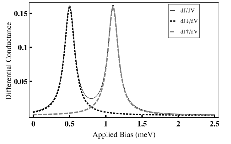
Figure 1: Differential conductance plot with respect to applied bias .Here $\epsilon_{\downarrow}(B)=0.5$ $meV$ , $\epsilon_{\uparrow}(B)=1$ $meV$ , $U=0.1~{}meV$ .$\Gamma=0.1$ $meV$.

Now we explain QD coupling with an oscillator in the presence of magnetic field. At zero temperature oscillator will be in ground state.As spin down electron comes onto QD it gives energy to oscillator and oscillator moves to excited state. This explain the phononic peaks appearance in differential conductance for spin down electrons. The main peak of spin down electron will get shifted due to $\left(\Delta\right)$ and amplitude of main peak of spin down electron becomes smaller as only spin down electron could give energy to oscillator in zero temperature. We have assumed strong dissipation effects with enviornment, which means as spin up or spin down electron leaves oscillator it comes to ground state. This rules out accumulation of energy in oscillator. When applied bias resonates with $\left(\epsilon_{\uparrow}+(m+\frac{1}{2})+U-\Delta\right)$ then spin up electron channel too get activated along with spin down electron channel. Here $\left(m\right)$represents number of phonons produced by spin down electron, and moreover spin up and spin down electrons have symmetric coupling with electrodes and QD $\left(\Gamma_{\uparrow}=\Gamma_{{}_{\downarrow}}\right)$ which means both spin up and spin down electrons comes onto QD and leaves the QD in the same time, and this is quite resonable as for identical metallic electrodes QD electrodes coupling strength will be same for both spin up and spin down electrons, This could be changed by using ferromagnetic leads52 . Therefore spin up electron excites oscillator to even more excited state.So we get satellite peaks in differential conductance of spin up electrons. Here phononic peaks of spin up and spin down electrons is not same. This happens as excited states of occupied QD coupled with oscillator eigen states are not same for different values of excitation.See Fig(2).

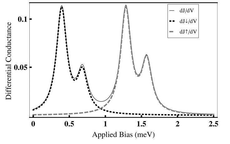
Figure 2: Differential conductance plot with respect to applied bias .Here $\epsilon_{\downarrow}(B)=0.5$ $meV$ , $\epsilon_{\uparrow}(B)=1$ $meV$ , $U=0.1~{}meV$ ,$\Gamma=0.3$ $meV$,$\alpha=0.37$ $meV$ ,$\omega=0.29$ $meV$.

Effects of  electrodes-QD coupling $\left(\Gamma s\right)$ in the presence of applied magnetic field and oscillator-QD coupling is of particular importance. As the tunneling rates of spin up and spin down electrons from electrodes to QD is increased then energy states of the QD gets broadened. In Fig.(3) we have showed that for a fixed value of applied  magnetic field and QD-oscillator coupling when electrodes-QD coupling are small than Zeeman splitted peaks and phononic side band peaks are clearly visible. But as we increase electrodes-QD coupling then phononic side band peaks starts disappearing.

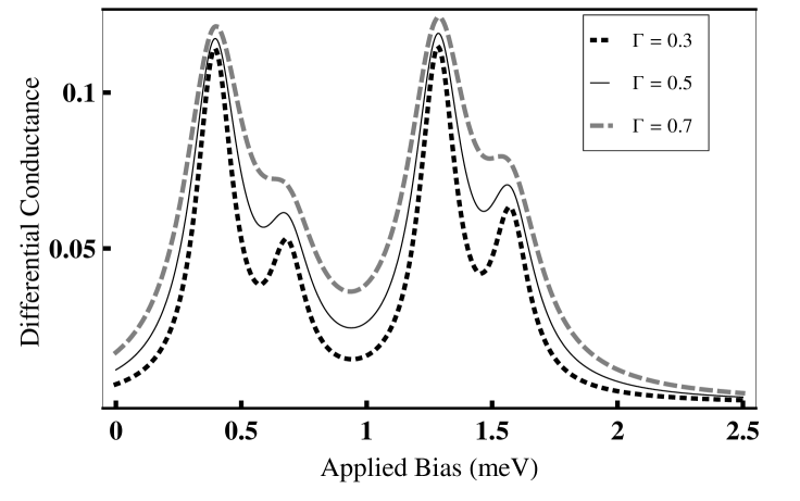
Figure 3: Differential conductance plot with respect to applied bias .Here $\epsilon_{\downarrow}(B)=0.5$ $meV$ , $\epsilon_{\uparrow}(B)=1$ $meV$ , $U=0.1~{}meV$ ,$\alpha=0.37$ $meV$ ,$\omega=0.29$ $meV$.

Average energy transferred to the oscillator by spin down and spin up electrons is shown in fig(4). Here we could see that spin down electron curve lies lower than spin up curve, where as small steps are signature of phonons creation in averge energy versus applied bias plot. Spin up electron starts contributing to increase average energy of oscillator where spin down electrons ends up, and applied bias resonates with $\left(\epsilon_{\uparrow}+(m+\frac{1}{2})+U-\Delta\right)$.

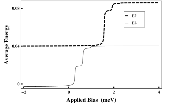
Figure 4: Average energy plot with respect to applied bias .Here $\epsilon_{\downarrow}(B)=0.5$ $meV$ , $\epsilon_{\uparrow}(B)=1$ $meV$ , $U=0.1~{}meV$ ,$\alpha=0.45$ $meV$ ,$\omega=0.35$ $meV$.

I.1 Conclusion

In this work we have studied inelastic electron transport through QD coupled with an nanomechancial oscillator in the presence of strong applied magnetic field. We have explained first spin down elctron creates phonon in QD and then spin up start creating phonons on it. Due to creation of phonons small steps are produced in average energy transferred to oscillator. With increasing electrodes QD coupling strength phononic satellite peaks starts hiding up.

I.2 Acknowledgment

M. Imran and K. Sabeeh would like to acknowledge the support of the Higher Education Commission (HEC) of Pakistan through project No. 20-1484/R&D/09.

${}^{{}^{\ast}}$imran1gee@gmail.com.

References

- (1) A. Schliesser, et. al., Nature Physics 5, 509 (2009).
- (2) K. L. Ekinci and M. L. Roukes, Review of Scientific Instruments 76, 061101 (2005).
- (3) K. L. Ekinci, Small 2005,1, No. 8-9, 786-797 (2005).
- (4) M. L. Roukes, Technical Digest of the 2000 Solid State Sensor and Actuator Workshop; “Nanoelectromechanical Systems”.
- (5) H. G. Craighead, Science 290, 1532 (2000).
- (6) P. Kim and C. M. Lieber, Science 126, 2148 (1999).
- (7) M. P. Blencowe, Phys. Rep. 395, 159 (2004).
- (8) A. N. Cleland, Foundations of Nanomechanics, 423, 2003 (Berlin:Springer).
- (9) R. G. Knobel and A. N. Cleland, Nature (London) 424, 291 (2003).
- (10) A. Naik et al., Nature (London) 443, 193 (2006).
- (11) Michael Galperin, Mark A. Ratner, Abraham Nitzan, Alessandro Troisi, Science 319, 1056 (2008).
- (12) H. Park, J. Park, A. K. L. Lim, E. H. Anderson, A. P. Alivisatos, and P.L. McEuen, Nature (London) 407, 57 (2000).
- (13) J. Koch and F. von Oppen, Phys. Rev. Lett. 94, 206804 (2005).
- (14) J. Koch, F. von Oppen, and A. V. Andreev, Phys. Rev. B 74, 205438 (2006).
- (15) M. Poot, E. Osorio, K. O’Neill, J. M. Thijssen, D. Vanmaekelbergh, C. A.van Walree, L. W. Jenneskens, and H. S. J. van der Zant, Nano Lett. 6,1031 (2006).
- (16) E. A. Osorio, K. O’Neill, N. Stuhr-Hansen, O. F. Nielsen, T. Bjørnholm, and H. S. J. van der Zant, Adv. Mater. (Weinheim, Ger.) 19, 281 (2007).
- (17) E. Lortscher, H. B. Weber, and H. Riel, Phys. Rev. Lett. 98, 176807 (2007).
- (18) A. Erbe, C. Weiss, W. Zwerger, and R. H. Blick, Phy. Rev. Lett. 87, 096106 (2001).
- (19) M. Poggio et al., Nature 4, 635 (2008).
- (20) S. J. Bunch, et al., Science 315, 490 (2007).
- (21) B. J. LeRoy et al., Nature 432, 371 (2004).
- (22) G. A. Steele, et al., Science 325, 1103 (2009).
- (23) A. D. Armour, M. P. Blencowe, and Y. Zhang, Phys. Rev. B 69, 125313 (2004).
- (24) A. D. Armour and A. MacKinnon, Phys. Rev. B 66, 035333 (2002).
- (25) Tomas Novotny, Andrea Donarini, Christian Flindt, and Antti-Pekka Jauho, Phys. Rev. Lett. 92, 248302 (2004).
- (26) T. Novotny, A. Donarini, and A.-P. Jauho, Phys. Rev. Lett. 90, 256801 (2003).
- (27) Christian Flindt, Tomas Novotny, and Antti-Pekka Jauho, Phys. Rev. B 70, 205334 (2004).
- (28) D. Wahyu Utami, et al., Phys. Rev. B 74, 014303 (2006).
- (29) A. Yu. Smirnov, L. G. Mourokh, and N. J. M. Horing, Phys. Rev. B 69, 155310 (2004).
- (30) D. Wahyu Utami, et al., Phys. Rev. B 70, 075303 (2004).
- (31) J. Villavicencio, et al., Appl. Phys. Lett. 92, 192102 (2008).
- (32) D. Fedorets, L. Y. Gorelik, R. I. Shekhter, and M. Jonson, Phys. Rev. Lett. 92, 166801 (2004).
- (33) L. V. Keldysh, Zh. Eksp. Teor. Fiz. 47, 1515 (1965).
- (34) H. Huagand and A. P. Jauho, Quantum Kinetics in Transport and Optics of Semiconductors, Springer Solid-State Sciences Vol. 123 (Springer, NewYork, 1996).
- (35) D. K. Ferry and S. M. Goodnick, Transport in nanostructure, CambridgeUniversity press, 2001., S. Datta, J. Phys.: Condens. Matter 2, 8023 (1990), R. Lake and S. Datta, Phys. Rev. B 45, 6670 (1992); 46, 4757 (1992).
- (36) D. Fedorets, L. Y. Gorelik, R. I. Shekhter, and M. Jonson, Europhys. Lett., 58, 99 (2002).
- (37) D. A. Ryndyk, R. Guti´errez, B. Song and G. Cuniberti, Springer Series in Chemical Physics, Volume 3, pages 213-235 (2009).
- (38) C. Caroli, R. Combescot, P. Nozieres, D. Saint-James, J. Phys. C: Solid St. Phys. 4, 916 (1971).
- (39) C. Caroli, R. Combescot, D. Lederer, P. Nozieres, D. Saint-James, J. Phys. C: Solid St. Phys. 4, 2598 (1971).
- (40) C. Caroli, R. Combescot, P. Nozieres, D. Saint-James, J. Phys. C: Solid St. Phys. 5, 21 (1972).
- (41) Y. Meir, N.S. Wingreen, Phys. Rev. Lett. 68, 2512 (1992).
- (42) N.S. Wingreen, A.P. Jauho, Y. Meir, Phys. Rev. B 48, 8487 (1993).
- (43) A.P. Jauho, N.S. Wingreen, Y. Meir, Phys. Rev. B 50, 5528 (1994).
- (44) C. B. Doiron, W. Belzig, and C. Bruder, Phys. Rev. B 74, 205336 (2006).
- (45) D. Mozyrsky, and I. Martin, Phys. Rev. Lett. 89, 018301 (2002).
- (46) Mozyrsky, I. Martin, and M. B. Hastings, Phys. Rev. Lett. 92, 018303 (2004).
- (47) M. Tahir and A. MacKinnon, Phys. Rev. B 77, 224305 (2008).
- (48) Michael Galperin, Abraham Nitzan, and Mark A. Ratner, Phys. Rev. B 74, 075326 (2006) ; 73, 045314 2006 ; V. Nam Do, P. Dollfus, and V. LienNguyen, Appl. Phys. Lett. 91, 022104 (2007) .
- (49) M. Galperin, M. A. Ratner, and A. Nitzan, J. Chem. Phys. 121, 11965 2004 ; Nano Lett. 4, 1605 (2004) .
- (50) Ned S. Wingreen, Karsten W. Jacobsen, and John W. Wilkins, Phys. Rev. B 40, 11834 (1989) .
- (51) Michael Galperin, Abraham Nitzan, and Mark A. Ratner, Phys. Rev. B 73, 045314 (2006) .
- (52) F M. Souza, Thiago L. Carrara, and E. Vernek,arXiv:1104.3483v1.
- (53) D.C.Langreth, in Linear and Nonlinear Electron Transport in Solids, Vol.17 of Nato Advanced Study Institute, Series B: Physics, edited by J.T Devreese and V.E. Van Doren (Plenum, New York, 1976).
- (54) J. Rammer and H. Smith, Rev.Mod.Phys. 58,323(1986).
- (55) A.P.Jauho, Solid State Electron.32,1265 (1989).
- (56) Quantum kinetics in transport and optics of semiconductors, Second substantially revised edition, Springer series in solid state science 123 by Hartmut J.W. Haugh and Antti Pekka Jauho.
- (57) Sebastian Schmitt and Frithjof B. Anders, PRL 107, 056801 (2011).
- (58) Toshimasa Fujisawa, Gou Shinkai, and Toshiaki Hayashi, Phys, Rev. B 76, 041302 (2007).
- (59) Eric R. Hedin and Yong S. Joe,J. Appl. Phys. 110, 026107 (2011).