General Quantum Fidelity Susceptibilities for the $J_{1}-J_{2}$ Chain

Abstract

We study slightly generalized quantum fidelity susceptibilities where the differential change in the fidelity is measured with respect to a different term than the one used for driving the system towards a quantum phase transition. As a model system we use the spin-$1/2$ $J_{1}-J_{2}$ antiferromagnetic Heisenberg chain. For this model, we study three fidelity susceptibilities, $\chi_{\rho}$, $\chi_{D}$ and $\chi_{\mathrm{AF}}$, which are related to the spin stiffness, the dimer order and antiferromagnetic order, respectively. All these ground-state fidelity susceptibilities are sensitive to the phase diagram of the $J_{1}-J_{2}$ model. We show that they all can accurately identify a quantum critical point in this model occurring at $J_{2}^{c}\sim 0.241J_{1}$ between a gapless Heisenberg phase for $J_{2}<J_{2}^{c}$ and a dimerized phase for $J_{2}>J_{2}^{c}$. This phase transition, in the Berezinskii-Kosterlitz-Thouless universality class, is controlled by a marginal operator and is therefore particularly difficult to observe.

I Introduction

The study of quantum phase transitions, especially in one and two dimensions, is a topic of considerable and ongoing interest.Sachdev (1999) Recently the utility of a concept with its origin in quantum information, the quantum fidelity and the related fidelity susceptibility, was demonstrated for the study of quantum phase transitions (QPT).Quan et al. (2006); Zanardi and Paunković (2006); Zhou and Barjaktarevič (2008); You et al. (2007) It has since then been successfully applied to a great number of systems.Zanardi et al. (2007a); Cozzini et al. (2007a, b); Buonsante and Vezzani (2007); Schwandt et al. (2009); Albuquerque et al. (2010) In particular, it has been applied to the $J_{1}-J_{2}$ model that we consider here. Chen et al. (2007). For a recent review of the fidelity approach to quantum phase transitions, see Ref. Gu, 2010. Most of these studies consider the case where the system undergoes a quantum phase transition as a coupling $\lambda$ is varied. The quantum fidelity and fidelity susceptibility is then defined with respect to the same parameter. Apart from a few studies, Zanardi et al. (2007b); Campos Venuti and Zanardi (2007); De Grandi et al. (2011) relatively little attention has been given to the case where the quantum fidelity and susceptibility are defined with respect to a coupling different than $\lambda$. Here we consider this case in detail for the $J_{1}-J_{2}$ model and show that, if appropriately defined, these general fidelity susceptibilities may yield considerable information about quantum phase transitions occurring in the system and can be very useful in probing for a non-zero order parameter.

Without loss of generality, the Hamiltonian of any many-body system can be written as

$$H(\lambda)=H_{0}+\lambda H_{\lambda},$$ (1)

where $\lambda$ is a variable which typically parametrizes an interaction and exhibits a phase transition at some critical value $\lambda_{c}$. In this form $H_{\lambda}$ is then recognized as a term that drives the phase transition.You et al. (2007) Using the eigenvectors of this Hamiltonian the ground-state (differential) fidelity can then be written as:

$$F(\lambda)=\left|\langle\Psi_{0}(\lambda)|\Psi_{0}(\lambda+\delta\lambda)\rangle\right|.$$ (2)

A series expansion of the GS fidelity in $\delta\lambda$ yields

$$F(\lambda)=1-\frac{(\delta\lambda)^{2}}{2}\frac{\partial^{2}F}{\partial\lambda^{2}}+\ldots$$ (3)

where $\partial_{\lambda}^{2}F\equiv\chi_{\lambda}$ is called the fidelity susceptibility. For a discussion of sign conventions and a more complete derivation see the topical review by Gu, Ref. Gu, 2010. If the higher-order terms are taken to be negligibly small then the fidelity susceptibility is defined as:

$$\chi_{\lambda}(\lambda)=\frac{2(1-F(\lambda))}{(\delta\lambda)^{2}}$$ (4)

The scaling of $\chi_{\lambda}$ at a quantum critical point, $\lambda_{c}$, is often of considerable interest and has been studied in detail and previous studies Zanardi et al. (2007b); Campos Venuti and Zanardi (2007); Gu and Lin (2009); Schwandt et al. (2009); Albuquerque et al. (2010) have shown that

$$\chi_{\lambda}\sim L^{2/\nu},\ \ \ \ \chi_{\lambda}/N\sim L^{2/\nu-d},$$ (5)

with $N=L^{d}$ the number of sites in the system. An easy way to re-derive this result is by envoking finite-size scaling. Since $1-F$ obviously is dimensionless it follows from Eq. (4) that the appropriate finite-size scaling form for $\chi_{\lambda}$ is

$$\chi_{\lambda}\sim(\delta\lambda)^{-2}f(L/\xi).$$ (6)

If we now consider the case where the parameter $\lambda$ drives the transition we may at the critical point $\lambda_{c}$ identify $\delta\lambda$ with $\lambda-\lambda_{c}$. It follows that $\xi\sim(\delta\lambda)^{-\nu}$. As usual, we can then replace $f(L/\xi)$ by an equivalent function $\tilde{f}(L^{1/\nu}\delta\lambda)$. The requirement that $\chi_{\lambda}$ remains finite for a finite system when $\delta\lambda\to 0$ then implies that to leading order $\tilde{f}(x)\sim x^{2}\sim L^{2/\nu}(\delta\lambda)^{2}$, from which Eq. (5) follows.

Here we shall consider a slightly more general case where the term driving the quantum phase transition is not the same as the one with respect to which the fidelity and fidelity susceptibility are defined. That is, one considers:

$$H(\lambda,\delta)=H_{1}+\delta H_{I},\ \ H_{1}=H_{0}+\lambda H_{\lambda}.$$ (7)

The fidelity and the related susceptibility is then defined as

$$F(\lambda,\delta) = \left|\langle\Psi_{0}(\lambda,0)|\Psi_{0}(\lambda,\delta)\rangle\right|,$$ (8)

$$\chi_{\delta}(\lambda) = \frac{2(1-F(\lambda,\delta))}{\delta^{2}}$$ (9)

The scaling of $\chi_{\delta}$ at $\lambda_{c}$ for this more general case was derived by Venuti et al.Campos Venuti and Zanardi (2007) where it was shown that:

$$\chi_{\delta}\sim L^{2d+2z-2\Delta_{v}},\ \ \ \chi_{\delta}/N\sim L^{d+2z-2\Delta_{v}}.$$ (10)

Here, $z$ is the dynamical exponent, $d$ the dimensionality and $\Delta_{v}$ the scaling dimension of the perturbation $H_{I}$. In all cases that we consider here $z=d=1$. We note that Eq. (10) assumes $[H_{1},H_{I}]\neq 0$, if $H_{I}$ commutes with $H_{1}$ then $F=1$ and $\chi_{\delta}=0$. The case where $H_{\lambda}$ and $H_{I}$ coincide is a special case of Eq. (10) for which $\Delta_{V}=d+z-1/\nu$ and one recovers Eq. (5).

A particular appealing feature of Eq. (5) is that when $2/\nu>d$, $\chi_{\lambda}/N$ will diverge at $\lambda_{c}$ and the fidelity susceptibility can then be used to locate the $\lambda_{c}$ without any need for knowing the order parameter. Secondly, it can be shown You et al. (2007); Zanardi et al. (2007b) that the fidelity susceptibility can be expressed as the zero-frequency derivative of the dynamical correlation function of $H_{I}$, making it a very sensitive probe of the quantum phase transition. Chen et al. (2008) On the other hand, if a phase transition is expected one might then use the fidelity susceptibility as a very sensitive probe of the order parameter through a suitably defined $H_{\delta}$ in Eq. (7). This is the approach we shall take here using the $J_{1}-J_{2}$ spin chain as our model system.

The spin-$1/2$ Heisenberg $J_{1}-J_{2}$ chain is a very well studied model. The Hamiltonian is:

$$H=\sum_{i}S_{i}\cdot S_{i+1}+J_{2}\sum_{i}S_{i}\cdot S_{i+2}$$ (11)

where $J_{2}$ is understood to be the ratio of the next-nearest neighbor exchange parameter over the nearest neighbor exchange parameter ($J_{2}=J_{2}^{\prime}/J_{1}^{\prime}$). This model is known to have a quantum phase transition of the Berezinskii-Kosterlitz-Thouless (BKT) universality class occurring at $J_{2}^{c}$ between a gapless ’Heisenberg’ (Luttinger liquid) phase for $J_{2}<J_{2}^{c}$ and a dimerized phase with a two-fold degenerate ground-state for $J_{2}>J_{2}^{c}$. Field theoryHaldane (1982); Eggert and Affleck (1992), exact diagonalizationTonegawa and Harada (1987); Eggert (1996) and DMRGChitra et al. (1995); White and Affleck (1996), have yielded very accurate estimates of the Luttinger Liquid-Dimer phase transition, the most accurate of these being due to EggertEggert (1996) which yielded a value of $J_{2}^{c}=0.241167$. Previous studies by Chen et al. Chen et al. (2007) of this model using the fidelity approach used the same term for the driving and perturbing part of the Hamiltonian as in Eq. (1) with the correspondence $H_{0}=\sum_{i}S_{i}\cdot S_{i+1}$, $H_{\lambda}=\sum_{i}S_{i}\cdot S_{i+2}$, $\lambda=J_{2}$.Chen et al. (2007) . Chen et al. demonstrated that, though no useful information about the Luttinger Liquid-Dimer phase transition could be obtained directly from the ground-state fidelity (and similarly the fidelity susceptibility), a clear signature of the phase transition was present in the fidelity of the first excited state.Chen et al. (2007) Sometimes this is taken as an indication that ground-state fidelity susceptibilities are not useful for locating a quantum phase transition in the BKT universality class. Here we show that more general ground-state fidelity susceptibilities indeed can locate this transition.

Specifically, we will study three fidelity susceptibilities, $\chi_{\rho}$, $\chi_{D}$ and $\chi_{\mathrm{AF}}$, which are coupled to the spin stiffness, a staggered interaction term and a staggered field term, respectively. In section II we present our results for $\chi_{\rho}$ while section III is focused on $\chi_{D}$ and section IV on $\chi_{\mathrm{AF}}$.

II The Spin Stiffness Fidelity Susceptibility, $\chi_{\rho}$

We begin by considering the $J_{1}-J_{2}$ model with $J_{2}=0$ but with an anisotropy term $\Delta$, what is usually called the $XXZ$ model:

$$H_{\mathrm{XXZ}}=\sum_{i}[\Delta S_{i}^{z}S_{i+1}^{z}+\cfrac{1}{2}(S_{i}^{+}S_{i+1}^{-}+S_{i}^{-}S_{i+1}^{+})].$$ (12)

The Heisenberg phase of this model, occurring for $\Delta\in[-1,1]$, is characterized by a non-zero spin stiffness Shastry and Sutherland (1990); Sutherland and Shastry (1990) defined as:

$$\rho(L)=\left.\frac{\partial^{2}e(\phi)}{\partial\delta^{2}}\right|_{\phi=0}.$$ (13)

Here, $e(\phi)$ is the ground-state energy per spin of the model where a twist of $\phi$ is applied at every bond:

$$H_{\mathrm{XXZ}}(\Delta,\phi)=$$

$$\sum_{i}[\Delta S_{i}^{z}S_{i+1}^{z}+\cfrac{1}{2}(S_{i}^{+}S_{i+1}^{-}e^{i\phi}+S_{i}^{-}S_{i+1}^{+}e^{-i\phi})].$$ (14)

The spin stiffness can be calculated exactly for the $\mathrm{XXZ}$ model for finite $L$ using the Bethe ansatz, Laflorencie et al. (2001) and exact expressions in the thermodynamic limit are available.  Shastry and Sutherland (1990); Sutherland and Shastry (1990) Interestingly the usual fidelity susceptibility with respect to $\Delta$ can also be calculated exactly. Yang (2007); Fjærestad (2008)

Since the non-zero spin stiffness defines the gapless Heisenberg phase it is therefore of interest to define a fidelity susceptibility associated with the stiffness. This can be done through the overlap of the ground-state with $\phi=0$ and a non-zero $\phi$. With $\Psi_{0}(\Delta,\phi)$ the ground-state of $H_{\mathrm{XXZ}}(\Delta,\phi)$ we can define the fidelity and fidelity susceptibility with respect to the twist in the limit where $\phi\to 0$:

$$F(\Delta,\phi) = \left|\langle\Psi_{0}(\Delta,0)|\Psi_{0}(\Delta,\phi)\rangle\right|,$$ (15)

$$\chi_{\rho}(\Delta) = \frac{2(1-F(\Delta,\phi))}{\phi^{2}}.$$ (16)

To calculate $\chi_{\rho}$ the ground-state of the unperturbed Hamiltonian was calculated through numerical exact diagonalization. The system was then perturbed by adding a twist of $e^{i\phi}$ at each bond and recalculating the ground-state. From the corresponding fidelity, $\chi_{\rho}$ was calculated using Eq. (16). Our results for $\chi_{\rho}/L$ versus $\Delta$ are shown in Fig. 1. For all data $\phi$ was taken to be $10^{-3}$ and periodic boundary conditions were assumed. In all cases it was verified that the finite value of $\phi$ used had no effect on the final results. The numerical diagonalizations were done using the Lanczos method as outlined by Lin et al. Lin (1990) Total $S^{z}$ symmetry and parallel programming techniques were employed to make computations feasible. Numerical errors are small and conservatively estimated to be on the order of $10^{-10}$ in the computed ground-state energies.

Figure 1: (Color online.) $\frac{\chi_{\rho}}{L}$ vs. $\Delta$: The spin stiffness fidelity susceptibility ($\chi_{\rho}(\Delta)/L$) as a function of the z-anistropy $\Delta$. At the $\Delta=0$ point the spin-current operator $\mathcal{J}$ and kinetic energy $\mathcal{T}$ commute with the XXZ Hamiltonian and thus such a perturbation does not change the ground-state, and the fidelity is one. Thus, $\chi_{\rho}$ is zero at this point.

In order to understand the results in Fig. 1 in more detail we expand Eq. (14) for small $\phi$:

$$H_{\mathrm{XXZ}}(\Delta,\phi)\sim H_{\mathrm{XXZ}}(\Delta)+\phi\mathcal{J}-\frac{\phi^{2}}{2}\mathcal{T}+\ldots,$$ (17)

$$\mathcal{J}=\frac{i}{2}\sum_{i}(S_{i}^{+}S_{i+1}^{-}-S_{i}^{-}S_{i+1}^{+}),$$ (18)

$$\mathcal{T}=\frac{1}{2}\sum_{i}(S_{i}^{+}S_{i+1}^{-}+S_{i}^{-}S_{i+1}^{+}).$$ (19)

Here, $\mathcal{J}$ is the spin current and $\mathcal{T}$ a kinetic energy term. The first thing we note is that, when $\Delta=0$ both $\mathcal{J}$ and $\mathcal{T}$ commute with $H_{\mathrm{XXZ}}(\Delta=0)$. The ground-state wave-function is therefore independent of $\phi$ (for small $\phi$) and $\chi_{\rho}\equiv 0$. This can clearly be seen in Fig. 1.

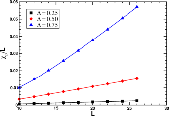
Figure 2: (Color online.) $\chi_{\rho}$ vs. $L$ (the XXZ model at different values of $\Delta$): This graph shows the scaling of $\chi_{\rho}$ with system size for different values of the z-anisotropy $\Delta$. The points represent numerical data and the lines represent fits to the scaling form predicted for the spin stiffness susceptibility $\chi_{\rho}/L=A_{1}L+A_{2}+A_{3}L^{-1}+A_{4}L^{3-8K}$. It can be seen that there is good agreement.

In the continuum limit the spin current $\mathcal{J}$ can be expressed in an effective low energy field theory Sirker et al. (2011) with scaling dimension $\Delta_{\mathcal{J}}=1$. However, we expect subleading corrections to arise from the presence of the operators $(\partial_{x}\Phi)^{2}$ with scaling dimension 2 and $\cos(\sqrt{16\pi K}\Phi)$ with scaling dimension $4K$. Here, $K$ is given by $K=\pi/(2(\pi-\mathrm{arcos}(\Delta)))$. For $\Delta\neq 0$ both of these terms will be generated by the term $\mathcal{T}$ in Eq. (17). Campos Venuti and Zanardi (2007) With these scaling dimensions and with the use of Eq. (10) we then find:

$$\chi_{\rho}/L=A_{1}L+A_{2}+A_{3}L^{-1}+A_{4}L^{3-8K}$$ (20)

In Fig. 2 a fit to this form is shown for 3 different values of $\Delta=0.25,0.5$ and $0.75$ in all cases do we observe an excellent agreement with the expected form with corrections arising from the last term $L^{3-8K}$ being almost un-noticeable until $\Delta$ approaches 1. We would expect the sub-leading corrections $L^{-1}$ and $L^{3-8K}$ to be absent if the perturbative term is just $\phi\mathcal{J}$.

We now turn to a discussion of a definition of $\chi_{\rho}$ in the presence of a non-zero $J_{2}$ but restricting the discussion to the isotropic case $\Delta=1$. In this case we define:

$$H(\phi)=$$

$$\sum_{i}[S_{i}^{z}S_{i+1}^{z}+\cfrac{1}{2}(S_{i}^{+}S_{i+1}^{-}e^{i\phi}+S_{i}^{-}S_{i+1}^{+}e^{-i\phi})]+$$

$$J_{2}\sum_{i}[S_{i}^{z}S_{i+2}^{z}+\cfrac{1}{2}(S_{i}^{+}S_{i+2}^{-}e^{i\phi}+S_{i}^{-}S_{i+2}^{+}e^{-i\phi})].$$ (21)

That is, we simply apply the twist $\phi$ at every bond of the Hamiltonian. As before we can expand:

$$H(\phi)\sim H(0)+\phi(\mathcal{J}_{1}+\mathcal{J}_{2})-\frac{\phi^{2}}{2}(\mathcal{T}_{1}+\mathcal{T}_{2})+\ldots,$$ (22)

$$\mathcal{J}_{1}=\frac{i}{2}\sum_{i}(S_{i}^{+}S_{i+1}^{-}-S_{i}^{-}S_{i+1}^{+}),$$ (23)

$$\mathcal{J}_{2}=\frac{i}{2}\sum_{i}(S_{i}^{+}S_{i+2}^{-}-S_{i}^{-}S_{i+2}^{+}),$$ (24)

$$\mathcal{T}_{1}=\frac{1}{2}\sum_{i}(S_{i}^{+}S_{i+1}^{-}+S_{i}^{-}S_{i+1}^{+}),$$ (25)

$$\mathcal{T}_{2}=\frac{1}{2}\sum_{i}(S_{i}^{+}S_{i+2}^{-}+S_{i}^{-}S_{i+2}^{+}).$$ (26)

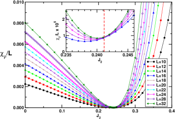
Figure 3: (Color online.) $\frac{\chi_{\rho}}{L}$ vs. $J_{2}$ and Inset: The generalized spin stiffness susceptibility, $\chi_{\rho}$ as a function of the second nearest-neighbor exchange coupling $J_{2}$. The system acquires a clearly size invariant form in the vicinity of the critical point $J_{2}\sim 0.24$ (as well as tending to a global minima). Inset shows the the minima for system sizes L=16,20,24,28,32 with $J_{2}^{c}$ indicated as the vertical dashed line. A clear dependence of the $J_{2}$ value of $\chi_{\rho}/L$ minima on the system size can be seen.

Our results for $\chi_{\rho}/L$ versus $J_{2}$ using this definition are shown in Fig. 3 for a range of $L$ from 10 to 32. In the region of the critical point at $J_{2}=0.241167$ the size dependence of $\chi_{\rho}/L$ vanishes yielding near scale invariance. How well this works close to $J_{2}^{c}$ is shown in the inset of Fig. 3. This alone can be taken to be a strong indication of $\chi_{\rho}/L$s sensitivity to the phase transition. In fact, this scale invariance works so well that one can locate the critical point to a high precision simply by verifying the scale invariance. This is illustrated in Fig. 4B where $\chi_{\rho}/L$ is plotted as a function of $L$ for $J_{2}=0.23$, $J_{2}=J_{2}^{c}$ and $J_{2}=0.25$. From the results in Fig. 4B the critical point $J_{2}^{c}$ where $\chi_{\rho}/L$ becomes independent of $L$ is immediately visible.

As can be seen in the inset of Fig. 3 $\chi_{\rho}/L$ reaches a minimum slightly prior to $J_{2}^{c}$. The $J_{2}$ value at which this minimum occurs has a clear system size dependence which can be fitted to a power-law and extrapolated to $L=\infty$ yielding a value of $J_{2c}=0.24077$. Hence, the minimum coincides with $J_{2}^{c}$ in the thermodynamic limit. This is shown in Fig. 4A. Comparison of this value with the accepted $J_{2}^{c}=0.241167$ reveals impressive agreement. Another noteworthy feature of the results in Fig. 3 is that $\chi_{\rho}/L$ is non-zero at the critical point, $J_{2}^{c}$. This value is very small but we have verified in detail that numerically it is non-zero.

The scale invariance of $\chi_{\rho}/L$ is clearly induced by the disappearance Eggert and Affleck (1992) of the marginal operator $\cos(\sqrt{16\pi K}\Phi)$ at $J_{2}^{c}$. We expect that in the continuum limit the absence of this operator implies that the spin current commutes with the Hamiltonian resulting in $\chi_{\rho}$ being effectively zero at $J_{2}^{c}$. The observed non-zero value of $\chi_{\rho}/L$ would then arise from short-distance physics.

Note that, as mentioned previously, we take the spin stiffness to be represented by a twist on every bond, both first and second nearest neighbor and not merely on the boundary as is sometimes done. This choice is not just a matter of taste. Imposing a twist only on the boundary (usually) breaks the translational invariance of the ground-state and, through extension, effects the value and behavior of the fidelity itself. Another point of note is the use of a twist of only $\phi$ between next-nearest neighbors. Geometric intuition would suggest that a twist of $2\phi$ should be applied between next-nearest neighbor bonds. However, for the small system sizes available for exact diagonlization it is found that a simple twist of $\phi$ on both bonds yields significantly better scaling.

Figure 4: (Color online.) A: The $J_{2}$ value of $\chi_{\rho}$ minima as a function of system size, as well as a (power law) line of best fit. As the system size tends towards infinity the power law best fit predicts a minima at $J_{2}=0.24077$ in good agreement with previously published results. B: Scaling of $\chi_{\rho}$ at $J_{2}=0.23$ (the highest, linear curve), $J_{2}=0.25$ (the second highest, linear curve) and at the critical point $J_{2}=0.241167$ (flat curve). The near constant scaling of $\frac{\chi_{\rho}}{L}$ at the critical point as well as non-constant scaling on either side of the critical point can clearly be seen.

III The Dimer Fidelity Susceptibility, $\chi_{D}$

We now turn to a discussion of a fidelity susceptibility associated with the dimer order present in the $J_{1}-J_{2}$ model for $J_{2}>J_{2}^{c}$. This susceptibility, which we call $\chi_{D}$, is coupled to the order parameter of the dimerized phase by design. Usually in the fidelity approach to quantum phase transitions one considers the case where the ground-state is unique in the absence of the perturbation. This is not the case here, leading to a diverging $\chi_{D}/L$ in the dimerized phase even in the presence of a gap. Specifically, we consider a Hamiltonian of the form:

$$H=\sum_{i}[S_{i}\cdot S_{i+1}+J_{2}S_{i}\cdot S_{i+2}+\delta h(-1)^{i}S_{i}\cdot S_{i+1}]$$

Thus, in correspondence with Eq. (7) we have $H_{I}=(-1)^{i}S_{i}\cdot S_{i+1}$ and we choose the driving coupling to be $J_{2}$. This perturbing Hamiltonian represents a conjugate field for the dimer phase. The scaling dimension of $H_{I}$ is known Affleck and Bonner (1990), $\Delta_{D}=\frac{1}{2}$, and from Eq. (10) we therefore find:

$$\chi_{D}\sim L^{4-2\Delta_{D}}=L^{3}\ \ (\mathrm{at}\ J_{2}^{c})$$ (28)

Due to the presence of the marginal coupling we cannot expect this relation to hold for $J_{2}<J_{2}^{c}$. However, the marginal coupling changes sign at $J_{2}^{c}$ and is therefore absent at $J_{2}^{c}$ where Eq. (28) should be exact. Eggert and Affleck (1992) For $J_{2}<0.241167$ it is knownAffleck and Bonner (1990) that logarithmic corrections arising from the marginal coupling for the small system sizes considered here lead to an effective scaling dimension $\Delta_{D}>\frac{1}{2}$. At $J_{2}=0$ Affleck and Bonner Affleck and Bonner (1990) estimated $\Delta_{D}=0.71$. Hence, using this results at $J_{2}=0$, we would expect that $\chi_{D}\sim L^{2.58}$ which we find is in good agreement with our results at $J_{2}=0$.

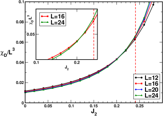
Figure 5: (Color online.) $\frac{\chi_{D}}{L^{3}}$ vs. $J_{2}$. The generalized dimer fidelity susceptibility $\chi_{D}/L^{3}$ as a function of the second nearest-neighbor exchange parameter $J_{2}$. A clear intersection of all curves can be seen in the vicinity of the proposed critical point at $J_{2}\sim 0.2-0.25$. The inset explicitly shows the crossing of $L=12$ and $L=24$. The dashed vertical lines indicate $J_{2}^{c}$.

We now need to consider the case $J_{2}>0.241167$. At $J_{2}=1/2$ the model is exactly solvable Majumdar (1970) and the two dimerized ground-states are exactly degenerate even for finite $L$. For $J_{2}^{c}<J_{2}<1/2$ the system is gapped with a unique ground-state but with an exponentially low-lying excited state. In the thermodynamic limit the two-fold degeneracy of ground-state is recovered, corresponding to the degeneracy of the two dimerization patterns. From this it follows that $\chi_{D}$ is formally infinite at $J_{2}=0$ and as $L\rightarrow\infty$ for $J_{2}^{c}<J_{2}<1/2$ we expect $\chi_{D}$ to diverge exponentially with $L$. At $J_{2}^{c}$ we expect $\chi_{D}$ to exactly scale as $L^{3}$ and for $J_{2}<J_{2}^{c}$ we expect $\chi_{D}\sim L^{\alpha}_{\mathrm{eff}}$ with $\alpha_{\mathrm{eff}}<3$. Hence, if $\chi_{D}/L^{3}$ is plotted for different $L$ we would expect the curves to cross at $J_{2}^{c}$. However, the crossing might be difficult to observe since it effectively arise from logarithmic corrections.

Our results for $\chi_{D}/L^{3}$ are shown in Fig. 5, where a crossing of the curves are visible around $J_{2}\sim 0.2-0.25$. As an illustration, the inset of Fig. 5 shows the crossing of $L=12$ and $L=24$. In order to obtain a more precise estimate of $J_{2}^{c}$ the intersection of each curve and the curve corresponding to the next largest system were tabulated ($L$ and $L+2$). These intersection points as a function of system size were then plotted Fig. 6A and found to obey a power-law of the form $a-bL^{-\alpha}$ with $\alpha\sim 1.8$ and $a=0.241$. This estimate of the critical coupling is in good agreement with the value of $J_{2}^{c}=0.241167$. Eggert (1996)

To further verify the scaling of $\chi_{D}$ at $J_{2}^{c}$ we show in Fig. 6B $\chi_{D}$ at $J_{2}^{c}$ as a function of the cubed system size, $L^{3}$. The strong linear scaling is in contrast to the scaling a small distance away from the critical point (not shown) where the scaling was found to be distorted by logarithmic corrections.

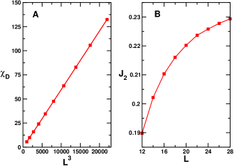
Figure 6: (Color online.) A: Scaling of $\chi_{D}$ vs. $L^{3}$ at the critical point $J_{2}=0.241167$. A near perfectly linear scaling is observed. B: The $J_{2}$ value of the intersection of $\frac{\chi_{D}}{L^{3}}$ between systems of size $L$ and $L+2$ plotted as a function of $L$. The curve can be fitted with a power-law line of best fit. The line of best fit is found to converge to $J_{2}=0.241$.

IV The AF Fidelity Susceptibility, $\chi_{\mathrm{AF}}$

Finally, we briefly discuss another fidelity susceptibility very analogous to $\chi_{D}$. We consider a perturbing term in the form of a staggered field of the form $\sum_{i}(-1)^{i}S^{z}_{i}$ with an associated fidelity susceptibility, $\chi_{\mathrm{AF}}$. The scaling dimension of such a staggered field is $\Delta_{\mathrm{AF}}=\frac{1}{2}$ and as for $\chi_{D}$ we therefore expect that $\chi_{\mathrm{AF}}\sim L^{3}$ at $J_{2}^{c}$. However, in this case it is known Affleck and Bonner (1990) that the effective scaling dimension for $J_{2}<J_{2}^{c}$ is smaller than $\frac{1}{2}$ resulting in $\chi_{\mathrm{AF}}\sim L^{\alpha_{\mathrm{eff}}}$ with $\alpha_{\mathrm{eff}}>3$ for $J_{2}<J_{2}^{c}$. On the other had, in the dimerized phase $\chi_{\mathrm{AF}}$ must clearly go to zero exponentially with $L$. Hence, if $\chi_{\mathrm{AF}}$ is plotted for different $L$ as a function of $J_{2}$ a crossing of the curves should occur.

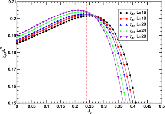
Figure 7: (Color online.) $\chi_{\mathrm{AF}}/L^{3}$ versus $J_{2}$. $\chi_{\mathrm{AF}}$ is expected to approach zero exponentially with the system size for $J_{2}>J_{2}^{c}$, to scale as $L^{3}$ at $J_{2}^{c}$ and to scale as $L^{\alpha_{\mathrm{eff}}}$ with $\alpha_{\mathrm{eff}}>3$ for $J_{2}<J_{2}^{c}$. A crossing close to the critical point $J_{2}^{c}$ (dashed vertical line) is then visible.

Our results are shown in Fig. 7 where $\chi_{\mathrm{AF}}/L^{3}$ is plotted versus $J_{2}$ for a number of system sizes. It is clear from these results that $\chi_{\mathrm{AF}}$ indeed goes to zero rapidly in the dimerized phase as one would expect. Close to $J_{2}^{c}$ the scaling is close to $L^{3}$ where as for $J_{2}<J_{2}^{c}$ it is faster than $L^{3}$. Hence, as can be seen in Fig. 7, a crossing occurs close to $J_{2}^{c}$.

V Conclusion and Summary

In this paper we have demonstrated the potential benefits of extending the concept of a fidelity susceptibility beyond a simple perturbation of the same term that drives the quantum phase transition. By using the spin-$1/2$ Heisenberg spin chain as an example we first created a susceptibility which was directly coupled to the spin stiffness but of increased sensitivity. This fidelity susceptibility, which we labelled $\chi_{\rho}$ can be used to successfully estimate the transition point at $J_{2}\sim 0.241$. Next we constructed another fidelity susceptibility, $\chi_{D}$, this time coupled to the order parameter susceptibility of the dimer phase. Again, we were able to estimate the critical point at a value of 0.241. Finally, we discussed an anti ferromagnetic fidelity susceptibility that rapidly approaches zero in the dimerized phase but diverges in the Heisenberg phase. Although susceptibilities linked to these quantities appeared the most useful for the $J_{1}-J_{2}$ model we considered here, it is possible to define many other fidelity susceptibilities that could provide valuable insights into the ordering occurring in the system being studied.