Supersonic and subsonic shock waves in the unitary Fermi gas

Abstract

We investigate shock waves in the unitary Fermi gas by using the zero-temperature equations of superfluid hydrodynamics. We obtain analytical solutions for the dynamics of a localized perturbation of the uniform gas. These supersonic bright and subsonic dark solutions produce, after a transient time, an extremely large (divergent) density gradient: the shock. We calculate the time of formation of the shock and also simulate the space-time behavior of the waves by solving generalized hydrodynamic equations, which include a reliable dispersive regularization of the shock. We find that the shock spreads into wave ripples whose properties crucially depend on the chosen initial configuration.

Degenerate Fermi gases Shock wave interactions and shock effects

One of the basic problems in physics is how density perturbations propagate through a material [1, 2]. In addition to the well-known sound waves, there are shock waves characterized by an abrupt change in the density of the medium [1, 2]. Shock waves are ubiquitous and have been studied in many different physical systems [1, 2]. Ten years ago shock waves have been experimentally observed also in atomic Bose-Einstein condensates (BECs) [3, 4, 5, 6], and theoretically investigated in various BEC configurations [7, 8, 9, 10, 11, 12, 13, 14]. Very recently the observation of nonlinear hydrodynamic waves has been reported in the collision between two strongly interacting Fermi gas clouds of ⁶Li atoms [15]. The experiment shows the formation of density gradients, which are nicely reproduced by hydrodynamic equations with a phenomenological viscous term [15]. Nevertheless, the role of dissipation is questionable [16] since the ultracold unitary Fermi gas is noted as an example of an almost perfect fluid [17]. Indeed in Ref. [16] it has been shown, by solving zero-temperature time-dependent Bogolibov-de Gennes equations, that the viscous term is not necessary to reproduce the experimental results of Ref. [15].

Here we investigate the formation and dynamics of shock waves in the dilute and ultracold unitary (divergent inter-atomic scattering length) Fermi gas by using the zero-temperature equations of superfluid hydrodynamics [1]. At zero temperature fermionic superfluids in the BCS-BEC crossover can be modelled by hydrodynamic equations [18] and their generalizations with a gradient term [19] that induces a dispersive regularization of the shock. In this paper we obtain analytical solutions for the dynamics of a localized perturbation of the uniform gas. We calculate the supersonic (or subsonic) velocity of propagation of these bright (or dark) perturbations. We show that bright perturbations evolve towards a shock-wave front, while dark perturbations produce the shock in their back, and we calculate the period $T_{s}$ of formation of the shock. In addition, we study the space-time behavior of the shock waves beyond this characteristic time $T_{s}$ by including a reliable quantum correction in the hydrodynamic equations [19]. In fact, according to the two-fluid model of Landau [1], the viscous term acts only on the normal component of the fluid, and at zero temperature the normal component is zero. Morover, recent theoretical microscopic calculations [20] suggest that the viscosity of the unitary Fermi gas is extremely small at very low temperatures because the transverse current does not couple to collective modes. By solving numerically these generalized equations of the unitary Fermi gas we show that the shock-wave front spreads into wave ripples whose properties crucially depend on the “brightness” (bright or dark) of the chosen initial configuration. We expect that our results are reliable when the normal density (with its viscous term) is quite small, i.e. for a temperature $T$ much smaller than the critical temperature $T_{c}$ of the normal-superfluid transition. For the unitary Fermi gas $T_{c}\simeq 0.2\ T_{F}$, where $T_{F}=\epsilon_{F}/k_{B}$ is the Fermi temperature with $k_{B}$ the Boltzmann constant, $\epsilon_{F}=\hbar^{2}(3\pi^{2}n)^{2/3}/(2m)$ the bulk Fermi energy of the ideal Fermi gas, $n$ the total density, and $m$ the mass of each atomic fermion. According to Ref. [21] for $T<0.1\ T_{F}$ the normal fraction is below $10\%$ and, in practice, in this range of temperatures our approach is fully justified.

At zero temperature the low-energy collective dynamics of a Fermi superfluid of neutral and dilute atoms at unitarity can be described by the equations of irrotational and inviscid hydrodynamics

$${\partial\over\partial t}n+\nabla\cdot(n{\bf v})=0\;,$$ (1)

$$m{\partial\over\partial t}{\bf v}+\nabla\Big{[}{m\over 2}v^{2}+\mu(n)+U({\bf r})\Big{]}={\bf 0}\;,$$ (2)

where $n({\bf r},t)$ is the total density of the superfluid, ${\bf v}({\bf r},t)$ is its velocity field, and

$$\mu(n)=\xi{\hbar^{2}\over 2m}(3\pi^{2})^{2/3}n^{2/3}$$ (3)

is the bulk chemical potential of the system, with $\xi\simeq 0.4$ a universal parameter [18]. Here we are supposing a balanced system, namely the same number of fermions in the two components of the spin ($\sigma=\uparrow,\downarrow$). The term $U({\bf r})$ models the external potential which traps the atoms.

Let us consider the unitary Fermi gas with constant density $\bar{n}$ with $U({\bf r})=0$. Experimentally this configuration can be obtained with a very large square-well potential (or a similar external trapping), such that in the model one can effectively impose periodic boundary conditions instead of the vanishing ones. A density variation along the $z$ axis with respect to the uniform configuration $\bar{n}$ can be experimentally created by using a blue-detuned (bright perturbation) or a red-detuned (dark perturbation) laser beam [22]. In practice, we perform the following factorization

$$n({\bf r})=n_{\bot}(x,y)\,n_{\parallel}(z)\;,$$ (4)

by imposing also

$$n_{\bot}(x,y)=\bar{n}_{\bot}$$ (5)

$$n_{\parallel}(z)=\bar{n}_{\parallel}\;\rho(z)$$ (6)

such that

$$n({\bf r})=\bar{n}\,\rho(z)$$ (7)

where $\bar{n}=\bar{n}_{\bot}\bar{n}_{\parallel}$, and $\rho(z,t)$ is the relative density, i.e. the localized axial modification with respect to the uniform density $\bar{n}$. We impose periodic boundary conditions along the $z$ axis, namely $\rho(z=L_{z},t)=\rho(z=-L_{z},t)$, with $2L_{z}$ the axial-domain length. We set ${\bf v}({\bf r},t)=(0,0,v(z,t))$ with $v(z,t)$ the velocity field such that $v(z=L_{z},t)=v(z=-L_{z},t)$. Moreover we impose that the initial localized wave packet satisfies the boundary conditions $\rho(z=\pm L_{z},t=0)=1$ and $v(z=\pm L_{z},t=0)=0$. Because the dimensional reduction is done assuming the uniformess in $x$,$y$ directions, we shall consider the propagation of a plane wave along the $z$ axis.

Inserting Eq. (7) into Eqs. (1) and (2) one finds the 1D hydrodynamic equations for the axial dynamics of the superfluid, given by

$${\dot{\rho}}+v\rho^{\prime}+v^{\prime}\rho=0\;,$$ (8)

$${\dot{v}}+vv^{\prime}+{c_{ls}(\rho)^{2}\over\rho}\rho^{\prime}=0\;,$$ (9)

where dots denote time derivatives, primes space derivatives, and

$$c_{ls}(\rho)=c_{s}\rho^{1/3}$$ (10)

is the local sound velocity, with $c_{s}=c_{ls}(1)=\sqrt{\xi/3}v_{F}$ the bulk sound velocity, $v_{F}=\sqrt{2\epsilon_{F}/m}$ is bulk Fermi velocity and $\epsilon_{F}={\hbar^{2}\over 2m}(3\pi^{2}\bar{n})^{2/3}$ the bulk Fermi energy.

The bulk sound velocity $c_{s}$ is the speed of propagation of a small perturbation $\tilde{\rho}(z,t)$ with respect to the uniform superfluid of density $\bar{n}$. In fact, setting $\rho(z,t)=1+\tilde{\rho}(z,t)$, with $\tilde{\rho}(z,t)\ll 1$ and $v(z,t)$ of the same order of $\tilde{\rho}(z,t)$, from the linearization of Eqs. (8) and (9) we get the familiar linear wave equation

$$\left({\partial^{2}\over\partial t^{2}}-c_{s}^{2}{\partial^{2}\over\partial z^{2}}\right)\tilde{\rho}(z,t)=0\;,$$ (11)

for $\tilde{\rho}(z,t)$ and a similar equation for $v(z,t)$. Modelling the initial perturbation with a Gaussian shape, i.e.

$$\tilde{\rho}(z,0)=2\eta\ e^{-z^{2}/(2\sigma^{2})}\;,$$ (12)

one finds [1, 2] from the linearized equations

$$\tilde{\rho}(z,t)=\eta\ e^{-(z-c_{s}t)^{2}/(2\sigma^{2})}+\eta\ e^{-(z+c_{s}t)^{2}/(2\sigma^{2})}\;,$$ (13)

with initial condition ${\dot{\tilde{\rho}}}(z,t=0)=0$. Thus, for the conservation of the linear momentum, the initial wave packet splits into two waves travelling in opposite directions with the speed of sound $c_{s}$. Obviously Eq. (13) is reliable only if $|\eta|\ll 1$. As expected, a small (infinitesimal) perturbation gives rise to sound waves.

We can find wave solutions of Eqs. (8) and (9) with a generic initial density profile by following the approach described by Landau and Lifshitz [1]. By supposing that the velocity $v$ depends explicitly on the density $\rho$, i.e. $v=v(\rho(z,t))$, one has ${\dot{v}}={dv\over d\rho}{\dot{\rho}}$, $v^{\prime}={dv\over d\rho}\rho^{\prime}$. We now impose that the two hydrodynamic equations reduce to the same hyperbolic equation

$${\dot{\rho}}+c(\rho)\rho^{\prime}=0\;,$$ (14)

where

$$c(\rho)=v(\rho)+{dv\over d\rho}\rho=v(\rho)+{c_{ls}(\rho)^{2}\over\rho}\left({dv\over d\rho}\right)^{-1}\;.$$ (15)

It is quite easy to verify that, given a initial condition $F(z)=\rho(z,t=0)$ for the density profile, the time-dependent solution $\rho(z,t)$ of the hyperbolic equation (14) satisfies the following implicit, but algebraic, equation:

$$\rho(z,t)=F(z-c(\rho(z,t))t)\;.$$ (16)

To determine the local velocity of propagation $c(\rho)$, which is not equal to the sound velocity $c_{ls}(\rho)$, we observe that from Eqs. (15) we get

$${dv\over d\rho}=\pm{c_{ls}(\rho)\over\rho}\;.$$ (17)

After separation of variables, and imposing that at infinity the density is equal to one and the velocity field is zero, we finally get

$$v(\rho)=\pm 3c_{s}(\rho^{1/3}-1)\;.$$ (18)

The velocity $c(\rho)$ follows directly from the velocity $v(\rho)$ by using Eqs. (15). One finds $c(\rho)=v(\rho)\pm c_{ls}(\rho)$, namely

$$c(\rho)=\pm c_{s}\left(4\rho^{1/3}-3\right)\;.$$ (19)

In conclusion, we have found that the density field $\rho(z,t)$ satisfies the implicit algebraic equation (16) with $c(\rho)$ given by Eq. (19). Note that a similar result, but with a very different local velocity, has been obtained by Damski [8] for the 1D BEC.

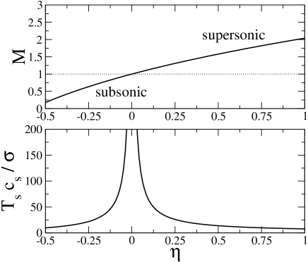
Figure 1: Properties of the shock waves. Upper panel: Mach number $M$ as a function of the amplitude $\eta$ of the perturbation (solid line). For $M<1$ there are subsonic and dark ($-1/2\leq\eta<0$) waves, while for $M>1$ there are supersonic and bright ($\eta>0$) waves. The dotted line separates the two regimes. Lower panel: period $T_{s}$ of formation (breaking time) of the shock-wave front as a function of the amplitude $\eta$ of the perturbation. $T_{s}$ is in units of $\sigma/c_{s}$, where $\sigma$ is the width of the perturbation and $c_{s}=\sqrt{\xi/3}v_{F}$ is the bulk speed of sound, with $v_{F}$ the Fermi velocity.

Eqs. (16) and (19) contain the dynamics of the two waves propagating to the left and to the right with initial condition (12). Some properties characterizing the dynamics can be extracted from these equations. First of all the two travelling waves have symmetric shapes during the time evolution. In addition, both amplitude and velocity of the extrema (maxima or minima, depending on the sign of $\eta$) of the two waves are practically constant during time evolution. In particular, the amplitude of the extrema is given by $A(\eta)=1+\eta$ while the velocity of the extrema reads

$$V(\eta)=c(1+\eta)=\pm c_{s}\left(4(1+\eta)^{1/3}-3\right)\;.$$ (20)

Notice that taking $\eta=0$ the velocity of the impulse extrema reduces to the sound velocity: $V(0)=c(1)=c_{s}=\sqrt{\xi/3}v_{F}$. Moreover, bright perturbations ($\eta>0$) move faster than dark ones ($\eta<0$), and the Mach number $M=V(\eta)/V(0)$ of these perturbations in the unitary Fermi gas is simply

$$M=4(1+\eta)^{1/3}-3\;.$$ (21)

For $M>1$, which means $\eta>0$ (bright perturbation), one has supersonic waves, while for $0\leq M<1$, which means $\eta<0$ (dark perturbation), one has subsonic waves. In the upper panel of Fig. 1 we plot the Mach number $M$ as function of the amplitude $\eta$ of the perturbation. Note that since $2\eta$ is the amplitude of the initial condition, see Eq. (12), the region $\eta\leq-1/2$ is unphysical.

Let us consider a bright perturbation ($\eta>0$) moving to the right. The speed of impulse maximum $V(\eta)$ is bigger than the speed of its tails $V(0)$. As a result the impulse self-steepens in the direction of propagation and a shock wave front takes place. The breaking-time $T_{s}$ required for such a process can be estimated as follows: the shock wave front appears when the distance difference traveled by lower and upper impulse parts is equal to the impulse half-width $2\sigma$, namely $[V(\eta)-V(0)]T_{s}=2\sigma$. This, by using Eqs. (19) and Eq. (10), gives

$$T_{s}={\sigma\over 2c_{s}((1+\eta)^{1/3}-1)}\;.$$ (22)

In the case of a dark perturbation ($\eta<0$) the tails of the wave packet move faster than the impulse minimum. The shock appears in the back of the travelling wave, and the period of shock formation is simply $T_{s}=2\sigma/(V(0)-V(\eta))$. In the lower panel of Fig. 1 we plot the period $T_{s}$ as a function of the amplitude $\eta$ of the perturbation. The figure shows that as $\eta$ goes to zero the period $T_{s}$ goes to infinity; in fact, in this limit the shock wave reduces to a sonic wave (sound wave) which does not produce a shock.

After the formation of the shock Eqs. (1) and (2) are not reliable because their exact solutions given of Eqs. (16) and (19) are no more single-valued. To overcome this difficulty we include a gradient quantum term in the hydrodynamic equations, which become

$${\partial\over\partial t}n+\nabla\cdot(n{\bf v})=0\;,$$ (23)

$$m{\partial\over\partial t}{\bf v}+\nabla\Big{[}{m\over 2}v^{2}-\lambda{\hbar^{2}\over 2m}{\nabla^{2}\sqrt{n}\over\sqrt{n}}+\mu(n)+U({\bf r})\Big{]}={\bf 0}\;,$$ (24)

We stress that at zero temperature the simplest regularization process of the shock is a purely dispersive quantum gradient term. Historically, the gradient term with $\lambda$ was introduced by von Weizsäcker to treat surface effects in nuclei [23]. This approach has been adopted for quantum hydrodynamics of electrons by March and Tosi [24], and also by Zaremba and Tso [25]. In the study of the BCS-BEC crossover the gradient term has been considered by various authors [26]. The choice of the parameter $\lambda$ in Eqs. (23) and (24) is still debated, here we choose $\lambda=1/4$, a value which gives good agreement with Monte Carlo calculations at zero and finite temperature (for details see [19, 21]). Moreover we set $\xi=0.4$.

We expect that Eqs. (23) and (24) are reliable to study the long-time dynamics of shock waves in the ultracold unitary Fermi gas. It is well known that, according to the two-fluid model and the Landau’s criterion of superfluidity [1], above a critical temperature $v_{c}$ a normal component with a dissipative term appears in the fluid [1]. As discussed in [27], for the unitary Fermi gas one has $v_{c}\simeq c_{s}$. Nevertheless, at ultrcold temperature the normal component is negligible and also the shear viscosity [17, 20]. For these reasons at zero temperature the shock waves are dispersive and not dissipative [16].

Eqs. (23) and (24) can be formally written (for any value of $\lambda$, also $\lambda=0$) in terms of a Galilei-invariant nonlinear Schrödinger equation [19]. Setting $U({\bf r})=0$ and using Eqs. (3) and (7) we easily get from Eqs. (23) and (24) a 1D nonlinear Schödinger equation. We solve this equation by using a Crank-Nicolson finite-difference predictor-corrector algorithm [28] with the initial condition given by Eq. (12) and $v(z,t=0)=0$. In fact, as also shown by Damski [8], we have verified that the initial velocity field $v(\rho(z,t=0))$ and $v(z,t=0)=0$ give practically the same time evolution.

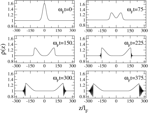
Figure 2: Time evolution of supersonic shock waves. Initial condition with $\sigma/l_{F}=18$ and $\eta=0.3$. The curves give the relative density profile $\rho(z)$ at subsequent frames, where $l_{F}=\sqrt{\hbar^{2}/(m\epsilon_{F})}$ is the Fermi length and $\omega_{F}=\epsilon_{F}/\hbar$ is the Fermi frequency.

In Fig. 2 we plot the time evolution of supersonic shock waves obtained with $\sigma/l_{F}=18$ and $\eta=0.3$, with $\sqrt{\hbar^{2}/(m\epsilon_{F})}$ the Fermi length of the bulk system. The figure displays the density profile $\rho(z)$ at subsequent times. Note the splitting on the initial bright wave packet into two bright travelling waves moving in opposite directions. As previously discussed, there is a deformation of the two waves with the formation of a quasi-horizontal shock-wave front. Eventually, this front spreads into wave ripples. There is no qualitative difference with respect to a Bose-Einstein condensate [8] in the physical manifestation of supersonic shock waves in the zero-temperature unitary Fermi gas. Nevertheless, due to the very different equation of state, there are large quantitative differences. Our numerical analysis confirms that the breaking time $T_{s}$ decreases by increasing the amplitude $\eta$, while the velocity $V$ of the maxima of the travelling waves increases by increasing $\eta$. There is a good agreement between our analytical formulas, Eqs. (20) and (22), and simulations: the relative difference is within $5\%$ for the velocity $V$ and within $20\%$ for the breaking time $T_{s}$.

In Fig. 3 we plot the time evolution of subsonic shock waves obtained again with $\sigma/l_{F}=18$ and $\eta=-0.2$. Also in this case the figure shows the splitting on the initial dark wave packet into two dark travelling waves moving in opposite directions. But here, as expected, the quasi-horizontal shock appears in the back side of the travelling waves. Our simulations show that for $\eta<0$ the wave ripples which appear at the breaking time $T_{s}$ are always dark, i.e. they never exceed the bulk density (compare wave ripples of Fig. 2 with those of Fig. 3). Note that dark shock waves have been studied long ago [29] in a different physical context: the discrete nonlinear Schrödinger equation. In that case the wave ripples can exceed the bulk density, probably due to the discrete nature of the Schrödinger equation. Also for dark shock waves our analytical predictions on velocity $V$ of the minima and breaking time $T_{s}$ are quite accurate with respect to numerical findings (similar relative differences of runs with $\eta>0$).

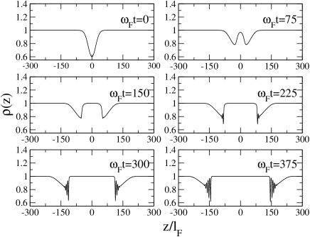
Figure 3: Time evolution of subsonic shock waves. Initial condition with $\sigma/l_{F}=18$ and $\eta=-0.2$. The curves give the relative density profile $\rho(z)$ at subsequent frames, where $l_{F}=\sqrt{\hbar^{2}/(m\epsilon_{F})}$ is the Fermi length and $\omega_{F}=\epsilon_{F}/\hbar$ is the Fermi frequency.

In conclusion, we have shown that at very low temperatures the unitary Fermi gas admits supersonic and subsonic shock waves, for which we have developed analytical and numerical results. Our predictions suggest a much cleaner method to produce shock waves with respect to the recent experiment [15] based on the collision of two ⁶Li atomic clouds. The shape of these waves changes during the time evolution giving rise to a shock-wave front at a characteristic breaking time. We have determined the Mach number of these travelling waves as a function of the perturbation amplitude, showing that supersonic bright and subsonic dark waves behave quite differently.

The author thanks Sadahn Kumar Adhikari, Tilman Enss, Boris Malomed, Enzo Orlandini, Mario Salerno, and Flavio Toigo for useful suggestions and discussions.

References

- [1] L.D. Landau and E.M. Lifshitz, Fluid Mechanics (Pergamon Press, London, 1987).
- [2] G.G. Whitham, Linear and Nonlinear Waves (Wiley, New York, 1974).
- [3] Z. Dutton, M. Budde, C. Slowe, and L.V. Hau, Science 293, 663 (2001).
- [4] M.A. Hoefer, M.J. Ablowitz, I. Coddington, E.A. Cornell, P. Engels, and V. Schweikhard, Phys. Rev. A 74, 023623 (2006).
- [5] J.J. Chang, P. Engels, and M.A. Hoefer, Phys. Rev. Lett. 101 170404 (2008); M.A. Hoefer, P. Engels, and J.J. Chang, Physica D 238, 1311 (2009).
- [6] R. Meppelink, S.B. Koller, J.M. Vogels, P. van der Straten, E.D. van Ooijen, N.R. Heckenberg, H. Rubinsztein-Dunlop, S.A. Haine, and M.J. Davis, Phys. Rev. A 80, 043606 (2009).
- [7] I. Kulikov and M. Zak, Phys. Rev. A 67, 063605 (2003).
- [8] B. Damski, Phys. Rev. A 69, 043610 (2004).
- [9] A.M. Kamchatnov, A. Gammal, and R.A. Kraenkel, Phys. Rev. A 69, 063605 (2004).
- [10] V.M. Perez-Garcia, V.V. Konotop, and V.A. Brazhnyi, Phys. Rev. Lett. 92, 220403 (2004).
- [11] B. Damski, Phys. Rev. A 73, 043601 (2006).
- [12] A. Ruschhaupt, A. del Campo, and J.G. Muga, Eur. Phys. J. D 40, 399 (2006).
- [13] L. Salasnich, N. Manini, F. Bonelli, M. Korbman, and A. Parola, Phys. Rev. A 75, 043616 (2007).
- [14] M.A. Hoefer, M.J. Ablowitz, and P. Engels, Phys. Rev. Lett. 100, 084504 (2008).
- [15] J. Joseph, J. Thomas, M. Kulkarni, and A. Abanov, Phys. Rev. Lett. 106, 150401 (2011).
- [16] A. Bulgac, Y.-L. Luo, and K.J. Roche, e-preprint arXiv:1108.1779.
- [17] C Cao, E Elliott, H Wu and J E Thomas, New J. Phys. 13, 075007 (2011).
- [18] S. Giorgini, L.P. Pitaevskii, and S. Stringari, Rev. Mov. Phys. 80, 1215 (2008).
- [19] L. Salasnich and F. Toigo, Phys. Rev. A 78 053626 (2008); L. Salasnich, Laser Phys. 19, 642 (2009); L. Salasnich and F. Toigo, Phys. Rev. A 82, 059902(E) (2010).
- [20] H. Guo, D. Wulin, C. C. Chien, and K. Levin, Phys.Rev.Lett. 107, 020403 (2011).
- [21] L. Salasnich, Phys. Rev. A 82, 063619 (2010).
- [22] H.J. Metcalf and P. van der Straten, Laser Cooling and Trapping (Springer, New York, 1999); C.J. Foot, Atomic Physics (Oxford University Press, Oxford, 2005).
- [23] C.F. von Weizsäcker, Zeit. Phys. 96, 431 (1935).
- [24] N.H. March and M. P. Tosi, Proc. R. Soc. A 330, 373 (1972).
- [25] E. Zaremba and H.C. Tso, Phys. Rrev. B 49, 8147 (1994).
- [26] Y.E. Kim and A.L. Zubarev, Phys. Rev. A 70, 033612 (2004); M.A. Escobedo, M. Mannarelli and C. Manuel, Phys. Rev. A 79, 063623 (2009); G. Rupak and T. Schäfer, Nucl. Phys. A 816, 52 (2009); S.K. Adhikari, Laser Phys. Lett. 6, 901 (2009); A. Csordas, O. Almasy, and P. Szepfalusy, Phys. Rev. A 82, 063609 (2010).
- [27] R. Combescot, M. Yu. Kagan, and S. Stringari, Phys. Rev. A 74, 042717 (2006); F. Ancilotto, L. Salasnich, F. Toigo, Phys. Rev. A 79, 033627 (2009).
- [28] E. Cerboneschi, R. Mannella, E. Arimondo, and L. Salasnich, Phys. Lett. A 249, 495 (1998); G. Mazzarella and L. Salasnich, Phys. Lett. A 373 4434 (2009).
- [29] V.V. Konotop and M. Salerno, Phys. Rev. E 56, 3616 (1997).