This paper presents a detailed proof of the triality theorem for
a class of fourth-order polynomial optimization problems. The
method is based on linear algebra but it solves an open problem on
the double-min duality left in 2003. Results show that the triality theory
holds strongly in a tri-duality form if the
primal problem and its canonical dual have the same dimension;
otherwise, both the canonical min-max duality and the double-max
duality still hold strongly, but the double-min duality holds
weakly in a symmetrical form.
Four numerical examples are presented to illustrate
that this theory can be used to identify not only the global minimum, but
also the largest local minimum and local maximum.
Key words and phrases:
canonical duality, triality, global optimization, polynomial
optimization, counter-examples.
1991 Mathematics Subject Classification:
90C26, 90C30, 90C46, 90C49
David Yang Gao
School of Science, Information Technology and Engineering,
University of Ballarat, Victoria 3353, Australia.
Changzhi Wu
School of Science, Information Technology and Engineering,
University of Ballarat, Victoria 3353, Australia.
School of Mathematics, Chongqing Normal University,
Shapingba, Chongqing, 400047, China
(Communicated by Kok Lay Teo)
1. Introduction and Motivation
The concepts of triality and tri-duality were
originally proposed in nonconvex mechanics [4, 5]. Mathematical theory of triality in its standard format
is composed of three types of dualities: a canonical min-max
duality and a pair of double-min and double-max dualities.
The canonical min-max duality
provides a sufficient condition for global minimum,
while the double-min and double max dualities can be used to
identify respectively the largest local minimum and local maximum.
The tri-duality is a strong form of the triality principle
[7]. Together with a canonical dual
transformation
and a complementary-dual principle, they comprise a versatile
canonical duality theory,
which can be used not only for solving a large class of challenging problems
in nonconvex/nonsmooth analysis and continuous/discrete optimization [7, 8],
but also for modeling complex systems and understanding multi-scale
phenomena within a unified framework [4, 5, 7]
(see also the review articles
[10, 12, 17]).
For example, in the recent work by Gao and Ogden
[13] on nonconvex variational/boundary value
problems, it was discovered that both the global and local
minimizers are usually
nonsmooth functions and cannot be determined easily by traditional Newton-type numerical methods.
However, by the canonical dual transformation, the nonlinear
differential equation is equivalent to an algebraic equation,
which can be solved analytically to obtain all solutions. Both
global minimizer and local extrema were identified by the triality theory, which revealed some interesting
phenomena in phase transitions.
The triality theory has attracted much attention recently in
duality ways: Successful applications in multi-disciplinary fields
of mathematics, engineering and sciences show that this theory
is not only useful and versatile, but also beautiful in its
mathematical format and rich in connotation of physics,
which reveals a unified intrinsic duality pattern in complex systems;
On the other hand,
a large number of
“counterexamples” have been presented in several papers since 2010. Unfortunately, most of these counterexamples are either
fundamentally wrong (see [30, 31]), or
repeatedly address an open problem left by Gao in 2003 on the double-min duality [9, 10].
The main goal of this paper is to
solve this open problem left in 2003.
The next section will present a brief review
and the open problem in the triality theory.
In Section 3, the triality theory is proved in its strong form
as it was originally discovered.
Section 4 shows that both the canonical min-max and the
double-max dualities hold strongly in general,
but the double-min duality holds weakly in a symmetrical form.
Applications are illustrated in Section 5, where a linear perturbation
method is used for solving certain critical problems.
The paper ended by an Appendix and a section of concluding remarks.
2. Canonical Duality Theory: A Brief Review and an Open Problem
Let us begin with the general global extremum problem
(1)
where is an open set,
is a decision vector, is a given symmetric
matrix, is a given
vector, and denotes a bilinear form on ; the function is
assumed to be nonconvex and differentiable (it is allowed to be
nonsmooth and sub-differentiable for constrained problems).
The notation stands for finding global extremal of the function given in .
In this paper, we are interested only in three types of global extrema:
the global minimum and a pair of the largest local minimum and local maximum.
Therefore, the nonconvex term in (1) is assumed
to satisfy the objectivity condition 111The concept of
objectivity in science means that qualitative and quantitative
descriptions of physical phenomena remain unchanged when the
phenomena are observed under a variety of conditions. That is, the
objective function should be independent with the choice of the
coordinate systems. In continuum mechanics, the objectivity is
also regarded as the principle of frame-indifference. See
Chapter 6 in [7] for mathematical definitions of the
objectivity and geometric nonlinearity in differential geometry
and finite deformation field theory. Detailed discussion of
objectivity in global optimization will be given in another paper
[18]., i.e., there exists a (geometrically)
nonlinear mapping and a canonical function such that
According to [7], a real valued function is said to be a canonical function on its
effective domain if its Legendre conjugate
(2)
is
uniquely defined on its effective domain such that the canonical duality relations
(3)
hold on , where
represents a bilinear form which puts and in
duality. The notation stands for solving the
stationary point problem in . By this one-to-one
canonical duality, the nonconvex function can be replaced by
such that the nonconvex function in (1) can be
written as
(4)
which is the so-called total
complementary (energy) function introduced by Gao and Strang in
1989. By using this total complementary function,
the canonical dual function
can be formulated as
(5)
where is called the
-conjugate of , defined by [7] as
(6)
Let be the feasible domain of
; then the canonical dual problem is to solve
the stationary point problem
Problem is a canonical dual to
in the sense that if is a critical
point of , then is a critical point of
, is a critical point of , and
(8)
Theorem 2.1 implies a perfect duality relation (i.e. no
duality gap) between the primal problem and its canonical
dual222The complementary-dual in physics means
perfect dual in optimization, i.e.,
the canonical dual in Gao’s work,
which means no duality gap. Otherwise, any duality gap will violet the energy conservation law.
Therefore, each complementary-dual variational statement in continuum mechanics
is usually refereed as a principle..
The formulation
of depends on the geometrical operator
.
In many applications,
the geometrical operator is usually a quadratic mapping
over a given field [7]. In finite dimensional space,
this quadratic operator can be written as a vector-valued
function (see [8], page 150)
(9)
where is a symmetrical matrix for each , and is defined by
In this case,
the total complementary function has the form
(10)
where is a matrix-valued function
defined by
(11)
The critical condition
leads to the
canonical equilibrium equation
(12)
Clearly, for any given if the vector , where stands for a space spanned by the columns of
, the canonical equilibrium equation (12) can
be solved analytically as333In this paper
should be understood as the generalized inverse if [8].. Therefore, the canonical dual
feasible space can be defined
as
Conversely, if is a critical solution of , it
must be in the form of (14) for a certain critical
solution of .
The canonical dual function for a general
quadratic operator was first formulated in nonconvex
analysis, where Theorem 2.2 is called the pure
complementary energy principle, [6]. In finite
deformation theory, this theorem
solved an open problem left by Hellinger (1914) and Reissner
(1954) (see [25]). The analytical solution theorem has
been successfully applied for solving a class of nonconvex
problems in mathematical physics, including Einstein’s special
relativity theory [7],
nonconvex mechanics and phase transitions in solids [13].
In global optimization, the primal solutions to
nonconvex minimization and integer programming problems are
usually located on the boundary of the feasible space.
By Theorem 2.2,
these solutions can be analytically determined by critical points
of the canonical dual function (see
[3, 11, 14, 16]).
In order to identify both global and local extrema of the primal
and dual problems, we assume, without losing much generality, that
the canonical function is convex
and let
(15)
(16)
where means that
is a positive semi-definite
matrix and means that
is negative definite.
If ,
then is a global
maximizer of Problem , the vector is
a global minimizer of Problem , and
the following canonical min-max duality statement holds:
(17)
If , then there exists a
neighborhood of for which we have either the double-min duality statement
(18)
or the double-max duality statement
(19)
The triality theory provides actual
global extremum criteria for three types of solutions to the
nonconvex problem :
a global minimizer if
and a pair of the largest-valued local extrema. In other words,
is the largest-valued local maximizer if is
a local maximizer; is the largest-valued local minimizer
if is a local minimizer.
This pair of largest local extrema plays a critical role in nonconvex
analysis of post-bifurcation and phase transitions.
Remark 1(Relation between Lagrangian Duality and Canonical Duality).
The main difference between the
Lagrangian-type dualities (including the equivalent Fenchel-Moreau-Rockfellar dualities)
and the canonical duality is
the operator .
In fact, if is linear, the primal problem is called geometrically linear
in [7] and the
total complementary function is simply the well-known Lagrangian
and is denoted as
(20)
In convex (static) systems, is linear and
is a saddle function. Therefore, the well-known saddle min-max
duality links a convex minimization problem to a concave maximization dual problem
with linear constraint:
(21)
where is the conjugate operator of defined via
.
Using the Lagrange multiplier to relax the equality constraint,
the Lagrangian is obtained.
By the fact that the (canonical) duality in convex static systems is unique, the saddle min-max
duality is refereed as the mono-duality in complex systems (see Chapter 1 in [7]).
Since the linear operator can not change the convexity of
, the Lagrangian duality theory can be
used mainly for convex problems. It is known that if
is nonconvex, then the Lagrangian duality as well as the related
Fenchel-Moreau-Rockafellar duality will produce the so-called
duality gap. Comparing the canonical dual function
in (13) with the Lagrangian dual function
in (21), we know that the duality gap
is .
The canonical duality theory is based on the (geometrically)
nonlinear mapping and the
canonical transformation .
The total complementary function
is also known as the nonlinear or extended
Lagrangian and is denoted by due to the geometric
nonlinearity of (see [7, 10]).
Relations between the canonical duality and the classical
Lagrangian duality are discussed in [16].
Remark 2(Geometrical Nonlinearity and Complementary Gap Function).
The canonical min-max duality statement (17) was first
proposed by Gao and Strang in nonconvex/nonsmooth analysis and mechanics
in 1989 [19], where is the so-called total potential energy with
representing the internal (or stored) energy and the
external energy.
The geometrical nonlinearity is a standard terminology in finite deformation theory,
which implies that the geometrical equation (or the configuration-strain relation)
is nonlinear.
By definition in physics, a function is called the
external energy means that its (sub-)differential must be the external force (or input)
. Therefore, in Gao and Strang’s work,
the external energy should be a linear function(al)
on its effective domain. In this
case, the matrix is a Hessian of the so-called complementary gap function (i.e. the Gao-Strang gap function
[19])
(22)
where is called the complementary operator of a Gâteauxdifferential of
[19]. Actually, in Gao and Strang’s original work,
the canonical min-max duality statement holds in a general (weak)
condition, i.e., in field theory (corresponding to the strong
condition ). The related canonical
duality theory has been generalized to nonconvex variational
analysis of a large deformation (von Karman) plate (where [34]), nonconvex (chaotic) dynamical systems
(where
[10]), and general nonconvex constrained
problems in global optimization.
Since in these general applications is the quadratic function ,
the Gao-Strang gap function (22) should be replaced
by the generalized form
(see the review article by Gao and
Sherali [17]).
This gap
function recovers the existing duality gap in traditional
duality theories and
provides a sufficient global optimality condition for general
nonconvex problems in both infinite and finite dimensional systems
(see review articles [10, 17]).
By the fact that the geometrical mapping in Gao and Strang’s work is a tensor-like
operator, it has been realized recently that the popular semi-definite programming method is actually a
special application (where is a quadratic function)
of the canonical min-max duality theory proposed in
1989 (see [14, 15]).
In a recent paper by Voisei and Zalinescu [31], they unfortunately
misunderstood some basic
terminologies in continuum physics, such as
geometric nonlinearity, internal and external energies, and
present “counterexamples” to the Gao-Strang theory based on certain “artificially chosen” operators
and quadratic functions .
Whereas in the stated contexts, the geometrical operator should be a canonical measure
(Cauchy-Reimann type
finite deformation operator, see Chapter 6 in [7])
and the external energy is typically a linear functional on its effective domain;
otherwise, its (sub)-differential will not be the external force.
Interested readers are
refereed by [18] for further discussion.
Remark 3(Double-Min Duality and Open Problem).
The double-min and double-max duality statements were
discovered simultaneously in a post-buckling analysis of large
deformed beam model [4, 5] in 1996,
where the finite
strain measure is a quadratic differential operator from a
2-D displacement field to a 2-D canonical strain field. Therefore,
the triality theory was first proposed in its strong form,
i.e. the so-called tri-duality theory (see the next section).
Later on when Gao was writing his duality book [7], he
realized that this pair of double-min and double-max dualities holds naturally
in convex Hamilton systems.
Accordingly, a bi-duality theorem was proposed and proved
for geometrically linear systems (where is a linear operator;
see Chapter 2 in [7]).
Following this, the triality theory was naturally generalized
to
geometrically nonlinear systems (nonlinear ; see Chapter 3
in [7]) with applications to global optimization
problems [8]. However, it was discovered in 2003
that if in the quadratic mapping
(9), the double-min duality statement needs
“certain additional constraints”. For the sake of mathematical
rigor,
the double-min duality was not included in
the triality theory and these additional constraints were left as
an open problem (see Remark 1 in [9], also Theorem
3 and its Remark in a review article by Gao [10]). By
the fact that the double-max duality is always true,
the double-min duality was still included in the triality theory
in the “either-or” form in many applications (see [12, 16]).
However, ignoring the open problem related to the “certain additional constraints” on the double-min duality statement has led to some misleading results.
The goal of this paper is to solve this open problem
by providing a simple proof of the triality theory based on linear
algebra.
To help understanding
the intrinsic characteristics of the original problem and its
canonical dual, we assume that the nonconvex objective function
is a sum of fourth-order canonical polynomials
(23)
where , are all symmetric
matrices, and are given constants.
This polynomial is actually a discretized form of the so-called
double-well potential, first proposed by van der Waals
in thermodynamics in 1895 (see [26]), which is the
mathematical model for natural phenomena of bifurcation and phase
transitions in
biology, chemistry, cosmology, continuum mechanics,
material science, and quantum field theory, etc.
(see [5, 20, 23, 24]).
By using the quadratic geometrical operator given
by (9),
the canonical function
(24)
and its Legendre conjugate
(25)
are quadratic functions, where represents the diagonal matrix defined by the non-zero
vector .
In the following discussions, we assume that all the critical
points of problem () are non-singular, i.e., if
, then
(26)
We will first prove that if , the triality theorem holds in
its strong form; otherwise, the theorem holds in its weak form.
Three numerical examples are used to illustrate the effectiveness
and efficiency of the canonical duality theory.
3. Strong Triality Theory for Quartic Polynomial Optimization: Tri-Duality Theorem
We first consider the case . For simplicity, we assume that
in the following discussion (otherwise,
can be replaced by and is replaced by
). In this case,
the problem (1) is denoted as problem (). Its canonical dual is
(27)
Theorem 3.1(Tri-Duality Theorem).
Suppose that , that the assumption (26) is
satisfied, that
is a critical point of Problem
and that .
If then is a global
maximizer of Problem in
if and only if is a global
minimizer of Problem , i.e.,
the following canonical min-max statement holds:
(28)
On the other hand, if , then,
there exists a neighborhood
of , such that either one of the
following two statements holds.
(A) The double-min duality statement
(29)
or (B) the double-max duality statement
(30)
Proof. If is a critical point of
the canonical dual problem , the criticality
condition
(31)
leads to . By the fact that ,
it follows that is
a critical point of Problem .
To prove the validity of the canonical min-max statement
(28), let be a critical point and
Since is concave
on , the critical point must be a global maximizer of on
.
For a fixed , the convexity of the complementary gap
function on leads to
(36)
Therefore, we have
(37)
This shows that is a global minimizer of Problem . Since it is assumed that
, it follows that (28) is
satisfied.
We move on to prove the double-min duality statement (29).
Let be a critical point of and
. It is easy to verify that
(38)
where
In light of (31), can be expressed in terms of as follows:
where is the identity matrix. If the critical point
is a local minimizer, we have This leads
to
(39)
Therefore, is positive definite
and is invertible. By
multiplying and to the left and
right sides of (39), respectively, we obtain
According to Lemma 6.2 in Appendix, the following matrix
inequality is obtained:
By the assumption (26), is also a
local minimizer of Problem
Therefore, on a neighborhood
of we have
Similarly, we can show that if is a local minimizer of
Problem the corresponding is also a local
minimizer of Problem
The next task is to prove the double-max duality statement
(30).
Let be a local maximizer of
Problem . Then, we have This gives us
(40)
Now we have two possible cases regarding the invertibility of
If is invertible, then by using a similar argument
as presented above, we can show that the relations
hold on a neighborhood
of .
If is not
invertible, by Lemma 6.1
in the Appendix, there exists
two orthogonal matrices and such that
(41)
where
and with and Substituting (41) into
(40), we obtain
(42)
Thus,
(43)
Applying Lemma 6.4 in Appendix to (43), it follows
that
Finally, we have
This means that is also a local maximizer of Problem under the assumption
(26), i.e., there exists a neighborhood of such that
Finally, we can show, in a similar way, that if is
a local maximizer of Problem and
,
the corresponding is also a local maximizer of
Problem Therefore, the tri-duality
theorem is proved.
Remark 4.
The strong triality Theorem 3.1 can also be used to identify
saddle points of the primal problem, i.e.
is a saddle point of if and only if
is a saddle point of
on .
Since the saddle points do not produce computational difficulties in
numerical optimization, and
do not exist physically in static systems, these points are excluded from
the triality theory.
Remark 5.
By the proof of Theorem 3.1, we know that if there exists a
critical point such that
is a local minimizer of Problem ,
then must be invertible. On the other hand,
if the symmetric matrices are linearly
dependent, then is not invertible for any
. In this case, the corresponding
canonical dual problem has no local
minimizers in , and for any critical point
, the analytical solution
is not a local minimizer of
.
4. Refined Triality Theory for General Quartic Polynomial Optimization
Let us recall the primal problem and its canonical dual problem
in the general quartic polynomial case ():
(44)
(45)
Suppose that
and are the critical points of Problem and Problem
respectively, where . It is easy to
verify that
(46)
(47)
In this case,
To continue, we show the following lemmas.
Lemma 4.1.
Suppose that . Let the critical point be a local minimizer of ,
and let . Then, there exists a matrix with such that
(48)
Proof. By the fact that the critical point
is a local minimizer of
, we have and
. It follows that
Thus, . Since and there exists a
non-singular matrix such
that
(49)
and
(50)
where and
According to the singular value decomposition theory
[22], there exist orthogonal matrices and
such that
Therefore, is an identity matrix. Let
Then,
Since ,
is an identity matrix, and is an
orthogonal matrix, we have
Thus, Note that
(51)
Let
. Then, we have
(52)
Let . Clearly, and . The proof is completed.
In a similar way, we can prove the following lemma.
Lemma 4.2.
Suppose that . Let be a critical point,
which is a local minimizer of Problem ,
where . Then, there exists a
matrix with
such that
(53)
Let be the column vectors of
and let be the column
vectors of , respectively. Clearly, are independent vectors and
are independent
vectors. We introduce the following two subspaces
(54)
(55)
Theorem 4.3(Refined Triality Theorem).
Suppose that the assumption (26) is satisfied. Let
be a critical point of and let .
If then the canonical min-max
duality holds in the strong form:
(56)
If , then there exists a
neighborhood of such that the double-max duality holds
in the strong form
(57)
However, the double-min duality statement holds conditionally in
the following super-symmetrical forms.
(1)
If and is a local
minimizer of , then is a
saddle point of and the double-min duality holds
weakly on , i.e.
(58)
(2)
If and is a local minimizer of
then is a saddle point of
and the double-min duality holds weakly on , i.e.
(59)
Proof. The proof of the statements
(56) and (57) are similar to that given for the proof of Theorem
3.1. Thus, it suffices to prove the double-min duality
statements (58) and (59).
Firstly, we
suppose that and is a local minimizer of Problem
.
Define
Thus, is a
non-singular matrix and . We claim that is
not a local minimizer of Problem On
a contrary, suppose that is also a local minimizer. Then,
we have
Thus, Since
and , it is clear that
This is a contradiction. Therefore, is a
saddle point of Problem .
It is easy to verify that .
Thus, to prove (58), it suffices to prove that is a local minimizer of the function
.
It is easy to verify that
(61)
and
(62)
In light of Lemma 4.1 and the assumption (26), it follows that
is, indeed, a local minimizer of the function .
In a similar way, we can establish the case of . The proof is
completed.
Remark 6.
Theorem 4.3 shows that both the canonical min-max and
double-max duality statements hold strongly for general cases; the
double-min duality holds strongly for but weakly for in a symmetrical form. The “certain additional conditions” are
simply the intersection for and
for . Therefore, the open
problem left in 2003 [9, 10] is solved for the
double-well potential function .
The triality theory has been challenged recently
in a series of more than seven papers, see, for example, [31, 32].
In the first version of [32], Voisei and Zalinescu wrote: “we consider
that it is important to point out that the main results of this
(triality) theory are false. This is done by providing elementary
counter-examples that lead to think that a correction of this
theory is impossible without falling into trivia”. It turns out
that most of these counter-examples simply use the double-well
function with . In fact,
these counter-examples address the same type of open problem for the double-min duality
left unaddressed in
[9, 10]. Indeed, by Theorem 4.3, we know
that both the canonical min-max duality and the double-max duality
hold strongly for the general case . However, based on
the weak double-min duality, one can easily construct other V-Z type counterexamples,
where the strong double-min duality
holds conditionally when . Also, interested readers
should find that the references [9, 10]
never been cited in any one of their papers.
5. Numerical Experiments
In this section, some simple numerical examples are presented to
illustrate the canonical duality theory.
Example 1 (). Let us first consider
Problem with .
(63)
where
The canonical dual problem can be expressed as
Thus,
and
Now, we take , and
. It is easy to check that has only one critical point in and four
critical points in ,
respectively. Furthermore, is a local minimizer and
is a local maximizer; the solutions and are saddle points of
in Thus,
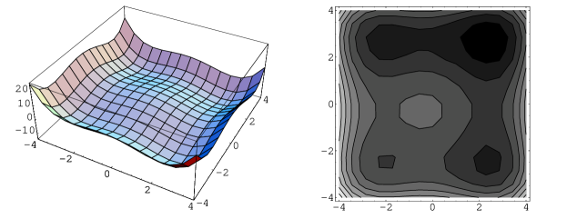
by Theorem 3.1, we know that is a global minimizer, while is a local minimizer and is a local maximizer. The corresponding
values of the cost function are
The graph of and its contour are depicted in
Figure 1.
Figure 1. Graph of (left) and contours of
(right) for Example 1
Example 2 (). We now consider Problem
with , , ,
, . Then, its dual problem is
We can verify that has one
critical point in and
two critical points and
in . Furthermore,
is a local minimizer and
is a local maximizer of . According to Theorem
4.3, is the unique global
minimizer of , is a saddle
point and is a local maximizer
of . Let and
. Then, it is
easy to verify that there exists neighborhoods and such
that ,
and
This example shows that even if , the canonical min-max
duality and the double-max duality still hold strongly. However,
the double-min duality statement should be refined into an
dimensional subspace in this case.
Example 3 (). We now consider Problem
with , , , , , and . Then, its
dual problem is
We can verify that has one
critical point in
and two critical points and in
. Furthermore, is a local maximizer and
is a saddle point of . According to
Theorem 4.3,
is the unique global minimizer of , is a local maximizer of
. Let and
.
Then, it is easy to verify that there exists neighborhoods
and such that , and
This example shows that if , the canonical min-max duality
and the double-max duality still hold strongly. However, the
double-min duality statement should be refined into an
dimensional subspace in this case.
Example 4 Linear Perturbation. Let us consider the following
optimization problem without input ()
Problem has four global minimizers
and the optimal cost value is Its canonical dual problem is
has only one critical point . Furthermore, we can check that is a local maximizer of Problem Thus, we cannot use the canonical dual
transformation method to obtain the global minimizer of Problem
since this problem is in a perfect
symmetrical form without input,
which allows more than one global minimizer. Now we perturb Problem as follows.
Its canonical dual function is expressed as
Taking , and solving the results obtained are
listed in Table 1. We can see that and
. Thus, is the global
minimizer of Problem .
Clearly, this is very close to . If we take
, the global minimizer of Problem
is which is close to . This example shows that if the
canonical dual problem has no critical point in
a linear perturbation could be used to
solve the primal problem.
Table 1. Numerical results for Example 3
6. Appendix
In this Appendix, we present several lemmas which are needed for
the proofs of Theorem 3.1 and Theorem 4.3.
In a similar
way, we can show that if then
The
proof is thus completed.
7. Conclusion Remarks
In this paper, we presented a rigorous proof of the double-min
duality in the triality theory for a quartic polynomial
optimization problem based on elementary linear algebra. Our
results show that under some proper assumptions, the triality
theory for a class of quartic polynomial optimization problems
holds strongly in the tri-duality form if the primal problem and
its canonical dual have the same dimension. Otherwise, both the
canonical min-max and the double-max still hold strongly, but
the double-min duality holds weakly in a symmetric form.
Acknowledgments
The main results of this paper were announced in the 2nd World
Congress of Global Optimization, July 3-7, 2011, Chania, Greece.
The authors are sincerely indebted to Professor Hanif Sherali at
Virginia Tech for his valuable comments and suggestions.
David Gao’s research is supported by US Air Force
Office of Scientific Research under the grant AFOSR
FA9550-10-1-0487.
Changzhi Wu was supported by National Natural
Science Foundation of China under the grant # 11001288, the Key
Project of Chinese Ministry of Education under the grant #
210179, SRF for ROCS, SEM, Natural Science Foundation Project of
CQ CSTC under the grant # 2009BB3057 and CMEC under the grant #
KJ090802.
References
[1]K.T. Andrews, M.F. M’Bengue and M. Shillor,
Vibrations of a nonlinear dynamic beam between two stops,
Discrete and Continuous Dynamical Systems - Series B, 12(1),
(2009), 23 - 38.
[2] I. Ekeland, and R. Temam,
“Convex Analysis and Variational Problems”,
North-Holland, 1976.
[3] S.C. Fang, D.Y. Gao, R.L. Sheu and S.Y. Wu, Canonical
dual approach for solving 0-1 quadratic programming problems,
J. Ind. and Manag. Optim. 4, (2008), 125-142.
[4]D.Y. Gao,
Post-buckling analysis and anomalous dual variational problems in nonlinear beam
theory in “Applied Mechanics in Americans Proc. of the Fifth Pan American
Congress of Applied Mechanics”, L.A. Godoy, L.E. Suarez (Eds.), Vol. 4.
The University of Iowa, Iowa city, August (1996).
[5] D.Y. Gao,
Dual extremum principles in finite deformation theory
with applications to post-buckling analysis of extended nonlinear beam
theory, Applied Mechanics Reviews, 50 (11), (1997), S64-S71.
[6] D.Y. Gao, General analytic solutions and complementary
variational principles for large deformation nonsmooth mechanics,
Meccanica 34, (1999), 169–198.
[7] D.Y. Gao,
“Duality Principles in Nonconvex Systems: Theory, Methods and
Applications”, Kluwer Academic, Dordrecht, 2000.
[8] D.Y. Gao, Canonical dual transformation method and
generalized triality theory in nonsmooth global optimization, J.
Glob. Optim., 17(1), (2000), 127–160.
[9] D.Y. Gao, Perfect duality theory and complete solutions
to a class of global optimization problems, Optim., 52(4–5),
(2003), 467–493.
[10] D.Y. Gao, Nonconvex semi-linear problems and canonical dual
solutions, In: Gao, D.Y., Ogden, R.W. (eds.) Advances in
Mechanics and Mathematics, vol. II, pp. 261 312. Kluwer Academic,
Dordrecht (2003).
[11] D.Y. Gao, Solutions and optimality to box constrained
nonconvex minimization problems, J. Ind. Manag. Optim. 3(2),
(2007), 293–304.
[12] D.Y. Gao, Canonical duality theory: theory, method, and
applications in global optimization, Comput. Chem., 33, (2009),
1964-1972.
[13] D.Y. Gao and R.W. Ogden, Multiple solutions to non-convex
variational problems with implications for phase transitions and
numerical computation, Quart. J. Mech. Appl. Math. 61 (4),
(2008), 497-522.
[14] D.Y. Gao and N. Ruan, Solutions to quadratic minimization
problems with box and integer constraints, J. Glob. Optim. 47(3),
(2010), 463-484.
[15] D.Y. Gao, N. Ruan,and P.M. Pardalos,
Canonical dual solutions to sum of fourth-order polynomials
minimization problems with applications to sensor network
localization, in Sensors: Theory, Algorithms and
Applications, P.M. Pardalos, Y.Y. Ye, V. Boginski, and C.
Commander (eds). Springer, 2010.
[16] D.Y. Gao, N. Ruan, and H. Sherali,
Solutions and optimality criteria for nonconvex constrained
global
optimization problems with connections between canonical and Lagrangian duality,
J. Glob. Optim. 45(3), (2009), 473-497.
[17] D.Y. Gao and H.D. Sherali, Canonical duality:
Connection between nonconvex mechanics and global optimization,
in Advances in Appl. Mathematics and Global Optimization,
249-316, Springer (2009).
[18] D.Y. Gao, H.D. Sherali, and G. Strang,
Canonical duality: Objectivity, Triality, and Gap functions,
in preparation.
[19] D.Y. Gao and G. Strang, Geometric nonlinearity:
Potential energy, complementary energy, and the gap function,
Quart. Appl. Math., 47(3), (1989), 487–504.
[20] D.Y. Gao, and H.F. Yu,
Multi-scale modelling and canonical dual finite element method in
phase transitions of solids,
International Journal of Solids and Structures, 45, (2008),
3660–3673.
[21] J. Gallier, The Schur complement and symmetric positive
semidefinite (and definite) matrices,
www.cis.upenn.edu/~ jean/schurcomp.pdf.
[22] R.A. Horn, and C.R. Johnson, “Matrix Analysis”, Cambridge
University Press, 1985.
[23] A. Jaffe,
Constructive quantum field theory, Mathematical Physics
2000,
111-127, Edited by A. Fokas, A. Grigoryan, T. Kibble, and B. Zegarlinski,
Imperial College Press, London 2000.
[24] T.W.B. Kibble,
Phase transitions and topological defects in the early
universe, Aust. J. Phys., 50, (1997), 697-722.
[25] S.F. Li and A. Gupta, On dual configuration
forces, J. of Elasticity, 84, (2006),13-31.
[26] J.S. Rowlinson,
Translation of J.D. van der Waals’
“The thermodynamic theory of capillarity under the
hypothesis of a continuous variation of density”, J. Statist.
Phys., 20, (1979), 197-244.
[27]N. Ruan, D.Y. Gao, and Y. Jiao
Canonical dual least square method for solving general
nonlinear systems of equations, Comput. Optim. Appl. 47 (2),
(2010), 335-347.
[28]D.M.M. Silva, and D.Y. Gao,
Complete solutions and triality theory to a nonconvex
optimization problem with double-well potential in , to
appear in J. Math. Analy. Appl.
[29] G. Strang, G.: Introduction to Applied
Mathematics, Wellesley-Cambridge Press, 1986, 758 pp.
[30] R. Strugariu, M.D. Voisei, and C. Zalinescu,
Counter-examples in bi-duality, triality and tri-duality,
http://www.math.uaic.ro/ zalinesc/papers3.php?file=svz.pdf
[31]M.D. Voisei, and C. Zalinescu,
Some remarks concerning Gao-Strang’s complementary gap
function, Applicable Analysis, (2010). DOI:
10.1080/00036811.2010.483427.
[32] M.D. Voisei, and C. Zalinescu, Counterexamples to some triality
tri-duality results, J. Glob. Optim., DOI 10.1007/s10898-010-9592-y.
[33] Z.B. Wang, S.C. Fang, D.Y. Gao,and W.X. Xing,
Canonical dual approach to solving the maximum cut problem,
to appear in J. Glob. Optim.
[34] S.T. Yau, and D.Y. Gao,
Obstacle problem for von Karman equations, Adv. Appl. Math.,
13, (1992),
123-141.
![[Uncaptioned image]](/html/1110.0293/assets/x2.png)